Does Marine Surface Tension Have Global Biogeography? Addition for the OCEANFILMS Package

Abstract

We apply principles of Gibbs phase plane chemistry across the entire ocean-atmosphere interface to investigate aerosol generation and geophysical transfer issues. Marine surface tension differences comprise a tangential pressure field controlling trace gas fluxes, primary organic inputs, and sea spray salt injections, in addition to heat and momentum fluxes. Mapping follows from the organic microlayer composition, now represented in ocean system models. Organic functional variations drive the microforcing, leading to (1) reduced turbulence and (by extension) laminar gas-energy diffusion; plus (2) altered bubble film mass emission into the boundary layer. Interfacial chemical behaviors are, therefore, closely reviewed as the background. We focus on phase transitions among two dimensional “solid, liquid, and gaseous” states serving as elasticity indicators. From the pool of dissolved organic carbon (DOC) only proteins and lipids appear to occupy significant atmospheric interfacial areas. The literature suggests albumin and stearic acid as the best proxies, and we distribute them through ecodynamic simulation. Consensus bulk distributions are obtained to control their adsorptive equilibria. We devise parameterizations for both the planar free energy and equation of state, relating excess coverage to the surface pressure and its modulus. Constant settings for the molecular surrogates are drawn from laboratory study and successfully reproduce surfactant solid-to-gas occurrence in compression experiments. Since DOC functionality measurements are rare, we group them into super-ecological province tables to verify aqueous concentration estimates. Outputs are then fed into a coverage, tension, elasticity code. The resulting two dimensional pressure contours cross a critical range for the regulation of precursor piston velocity, bubble breakage, and primary aerosol sources plus ripple damping. Concepts extend the water-air adsorption theory currently embodied in our OCEANFILMS aerosol emissions package, and the two approaches could be inserted into Earth System Models together. Uncertainties in the logic include kinetic and thermochemical factors operating at multiple scales.

1. Introduction

Composition of the marine atmospheric interface determines the surface tension across most of the ocean [1,2,3,4,5,6,7,8,9] so that multiple climate-critical fluxes are influenced. Transfer of trace greenhouse and aerosol-source gases, organic and sea salt aerosol mass, momentum, heat, and water vapor are all defined by gradients in tension at the sea-air boundary [10,11,12,13,14,15]. It has long been suspected that concentration patterns of detrital, surface-active biomacromolecules exert key control over ocean microlayer dynamics. Therefore, the structural type and geographical distribution of macromolecules must be known to determine the two-dimensional forces being imparted [6,16,17,18,19]. Several attempts have been made to simulate the geophysical effects of surfactants at the level of Earth system modeling by assuming proportionality of the biomacromolecules to chlorophyll [20,21,22,23,24]. The pigments are detectable from space and track phytoplankton, allowing for some level of connection to be made. Remote sensing has proven to be a reasonable starting point, but detailed microchemical information remains lacking.

Since organic structural types partially determine the composition of sea spray particles [4,25,26,27,28,29], our own aerosol-oriented group has recently become interested in constructing geographical distributions for individual classes of macromolecule. Our initial angle for this task has been that of adsorption—upper ocean surface films accumulate through both surfactant equilibration and the physicochemical competition for microlayer sites. Such processes regulate both organic and sea salt mass entering primary marine aerosol modes through bubble rupture [30,31,32,33]. Isotherms representing the types of surfactant covering bubble interfaces have been tested, then inserted into global biogeochemistry calculations. Full modern mapping techniques are now applied and the total package is referred to by the acronym OCEANFILMS [30,31]. Improvements to the simulation of primary aerosol mass have already been realized [31].

However, adsorption of macromolecules also implies alterations to the surface tension, a fundamental property of the physicochemical plane dividing the ocean from the atmosphere. Such changes can be represented through classic two-dimensional (Gibbsian) equivalency of the chemical potential [5,34,35,36,37]. In the present work, we extend the adsorptive surfactant calculations and construct chemically-derived global patterns to assess the role of macromolecules operating through film tension, or, more traditionally, two-dimensional pressure (tangential [2,36,38]). Crude, ideal equations of state are constructed and applied to the global ocean marine microlayer. We perform this mapping exercise first at the scale of marine biogeochemical provinces [39,40], selecting and grouping them to optimize a measurement base. Offline semi-dynamic biogeochemistry calculations are then conducted as a further test of the methodology [33,41,42,43]. These are coupled to a surface pressure-area parameterization. Emphasis is placed upon the two most basic issues involved: will geographic differences in surface tension be identifiable-computable? And will they be important to the many geochemical and climate-relevant fluxes with which they have been connected?

2. Background

It has been known for millennia that when certain organic liquids spread over the natural water-air boundary they can exert a calming effect on waves of many scales [9,17,44]. There have, in fact, been numerous documented attempts to actively, chemically de-engineer harbor mouth and shipping lane breakers. Some of these date back hundreds of years (see [45,46] and the technical histories provided therein). During and after the World Wars it became clear that surfactant influence on upper ocean mixing must also function on regional to planetary scales [47,48,49] and, furthermore, that it extends to the turbulent eddy spectrum arising around the atmospheric interface [38,50]. This latter connection implies influence upon large-scale transfer of many other properties—e.g., ocean solute mass inclusive of dissolved gas concentration gradients, heat, energy and, also via temperature dependence of the vapor pressure, water itself [2,46,51]. Soon afterward the logic was adapted to the control that surfactant-tension has on bubbles, disruptive film dispersal, and spray distributions [25,52,53,54]. Effects on trace gas fluxes operating in the greenhouse and marine aerosol-cloud systems began to draw real attention only during the era of global change biogeochemistry [2,6,55].

The physical mechanisms to which surfactant control applies include (to offer a set of partial examples)—Prandtl, Monin-Obhukov, Gibbs-Marangoni, laminar renewal, and viscoelastic and microlayer rheological theories. The coupling of fluid dynamics with environmental organic chemistry is perhaps one reason such concepts have been slow to take hold within Earth system models. We have collected some of the clearer explanations available for connections within the physical system [17,18,46,50,56,57,58,59,60,61], in order to provide justification for our geochemical mapping efforts. The detailed approach presented later, however, remains purely empirical. We now provide the reader with a heuristic summary of surfactant influence on atmospheric and oceanographic mixing, incorporating film tension factors. The present work then discusses the potential biological, geochemical, and ecogeographic distinctions. It is argued that the latter are strong enough to be of interest in the context of boundary layer vertical transport as handled in Earth system models.

A monomolecular layer of appropriately mixed organics may exert unexpected control on any and all fluid movement near the sea-air interface [8,45,46,48,59,61]. The arguments are not exclusive to the upper ocean—atmospheric mixing along with gas, particle, and energy fluxes are included moving well into the troposphere [60]. Working from the geometric top of the relevant environment downward as a conceptual device, it is often noted that surfactants begin by suppressing the capillary (centimeter-scale) waves that act upon boundary layer meteorology as roughness elements [8,9,18,59,62,63,64,65]. This occurs through modified hydrodynamic boundary conditions allowing for energy dispersion at certain key frequencies [17,56]. The normal cascade of momentum flow and turbulent exchange from the atmosphere into the sea is interrupted. In some cases it may be shut off almost completely, leading to a reduction in the vertical interchange within only minutes [45,46,59]. A readily observable glassy slick will often follow, sometimes extending over large areas. This may last for many hours and be detectable at altitude or from space [8,12,38,64]. The crucial chemical dependence of the effect is common knowledge to the shipping industry, because oily waste materials ejected at the water line are only sometimes calming [45,46].

Simultaneously, eddies approaching the water-air interface alternately dilate and compress the border running between the ocean and atmosphere [18,38]. Turbulent structures along the surface experience energy loss or extraction due to elasticity gradients through the microlayer. These follow from the presence of the macromolecules and biopolymers, for which distributions are patchy in both spatial and chemical senses. The effect may be tightly confined locally, but on the average it can also extend over hundreds of kilometers [6,8,18,59,64]. Multi-scale tension gradients are dominant across geophysical dynamic interfaces, and are attributed to variability (heterogeneity) in the natural surfactant distribution [9,19,64]. The process of extracting energy from eddies may also modulate the thicknesses of several hypothetical laminar layer barriers, stacked on top of one another in the liquid and gas phases. These regulate all manner of mass and energy transfer. Marine aerosol emissions offer the highest profile examples, but here we begin to discuss turbulence as well. Surface renewal constitutes a rate determining step in numerous climate relevant geocycles. The flow of greenhouse- or aerosol-forming trace gases, and either sensible or latent heat, may be blocked [6,9,50,51,60]. Water vapor is affected through skin temperature because this sets the vapor pressure [2,51,66,67]. Vivid demonstrations have been documented over many generations—sometimes accidentally, sometimes intentionally, within laboratories, witnessed in the field, or even detected from space up to the largest scales [6,18,28,45,46,50,59,64].

Our current mapping effort must necessarily rely on surfactant physicochemical concepts unfamiliar to contemporary students of global change. The approach is very strictly reduced in its dimensionality, so that it constitutes nonstandard environmental chemistry. The atmospheric, geographic problem set involved is highly understudied—opportunities may be expected. Our subject matter is, by its very nature, cross-disciplinary. The regulatory surfactants in question position their hydrophilic head groups within seawater proper. The remainder of their molecular structures, plus a significant amount of chemical activity, impact the gas phase directly. Longer organic moieties are capable of participating in oxidative radical photochemistry in the lowest few nanometers of the planetary atmosphere. However, for our purposes here, we will focus on the particulate source and any energetic flux tuning. Marine ecological information is transferred to the piston velocities underlying dimethyl sulfide and purely organic secondary emissions [2,27,32,55], to the fragmentation regime during bursting of bubble films, [28,29] and to sea salt and primary organic injections [27,28,29,30,31,32]. We are hopeful due to the latter that parameterizations developed here can contribute to our accumulating OCEANFILMS literature which, thus far, has been limited exclusively to Langmuir adsorption [30,31,32,33].

As noted in the introduction, we endeavor to establish only that surface tension differences can, in fact, be mapped, and that they are sufficiently strong to matter in a quantitative sense. We show that across key spatiotemporal transitions, and over ocean basin scales, two-dimensional pressure gradients in the Gibbs plane probably surpass known thresholds for variations in the laminar gas layer, bubble film mass injection, frictional fluxes, and more [16,17,18,19,20,21,27,28,29,30,31,32,56,57,58,59,60,61]. The composition distributions themselves turn out to be difficult to verify. Neither the macromolecules nor their functionality can yet be monitored by satellite and, furthermore, they have not entered the geochemical and geophysical flux parameterizations common to most Earth system models. Under such circumstances, chemically-resolved measurements remain rare. The available upper ocean functional data have been explored relatively completely in our OCEANFILMS work [30,31,32,33], but this only serves as a starting point. In the present text we attempt to move beyond concentration and adsorption to full simulation of a planetary, two-dimensional, interfacial equation of state. Thus, the current text can be considered completely distinct even from our foundation literature, and we draw in analyses of the surface tension itself.

As a theoretical preparation, we recommend, from recent experience, our own methodology. This has been to harvest selectively from high-profile, multidisciplinary textbook and monograph treatments appearing regularly over the decades. Information must be combined from several well-established, but disjoint, research communities. Chemical engineers first dissected surfactant to eddy relationships for generalized liquid–vapor systems in the 1950s, and the media were often environmentally relevant because they tended to be aqueous and ionic [36,38]. During the advent of global marine atmospheric chemistry studies, ambient organic measurements began to be linked to the wide variety of geophysical fluxes—at least along coastlines [2,12], and there continues to be concern in the modern era for surface chemical aspects of coupled climate feedback processes [14,15].

3. Methods and Theory

Stages in the project are now summarized in bullet form as an organizational device. Interfacial (tangent) force issues appear early in the list, and we follow up immediately with key definitions. These further serve as a concise preview, for theory applied in the calculations but developed more fully in Appendix A. Major steps in our exploration have been:

• List observed (2D) surface pressure ranges and influence on: (Section 4)

  ◦

  Aerosol emissions and gas precursor piston velocities [18]

  ◦

  Sea salt spray injection including primary organics [28]

  ◦

  Capillary wave modulation to the drag coefficient [46]

• Define a surface pressure range (0.3 to 3 mN/m) encompassing all effects (

  Table 1. A sampling of global ocean (2D) surface pressure ranges along with documented influence on several parameters related to sea-air flux types. All processes are dominated by the biomacromolecular surfactant effects cited here. While reduction mechanisms trace to the elastic modulus, surface tension is more often reported and the two quantities are interconnected. Uncertainties in the “effect” column constitute another factor of approximately three above the π range. As explained in the text, for the spray flux case the sign of the effect has not been established.

  Phenomenon	Measured π	Parameter	Effect	References/Authors
  Trace Gas Transfer	0.3–3 mN/m	Piston Velocity	Lower 3x	Davies 1966 and 1972; Goldman et al. 1988; Frew 1997; Tsai and Liu 2003, Frew et al. 2006; Bell et al. 2013
  Sea Spray Flux	1–10 mN/m	Number or Efficiency	±3x	Blanchard 1963; Garrett 1968; Paterson and Spillane 1969; Detwiler and Blanchard 1978; Lewis and Schwartz 2004; Modini et al. 2013; Alpert et al. 2015
  Ripples/Capillaries	0.3–3 mN/m	Damping e-Fold Distance	Lower 3x	Garrett 1967; Jarvis et al. 1967; Ermakov et al. 1986; Wei and Wu 1992; Bock and Frew, 1993; Hunter 1997; Dysthe 2006
  Boundary Wind	>1 mN/m (so above background)	Drag Coefficient	Lower 3x	Hicks et al. 1974; Deacon 1979; Ermakov et al. 1986; Asher 1997; Mitsuyasu and Bock 2001; Simpson et al. 2014; Cox et al. 2016

  )
• Segregate and prioritize global biomacromolecules by their likely functionality (Section 5) [30,31,32,33,37]

  ◦

  It is concluded that proteins and lipids dominate air-water interfaces

• Choose the best proxies as model surfactants (Section 6) [38,63]

  ◦

  Albumin (protein) and stearic acid (lipids)

  ◦

  Standard commercial alternatives are rejected

• Estimate global mixed layer concentrations of proteins and lipids in the context of systems models (with marine ecodynamics—Section 7) [30,31,32,33]
• Construct a 2D equation of state to provide surface pressure values as a function of surfactant occupancy (Section 8 and Appendix A) [36,38]

  ◦

  Absolute 2D pressures agree broadly with limited measurement data at local to biome scales (Section 8) (e.g., [1,2,3,4,5,39,40])

  ◦

  Global organic functionality is estimated offline from systems models, producing complete maps and sensitivity visualizations (Section 9)

• We address the two introductory questions: (Section 9 and remainder)

  ◦

  Distributions of 2D pressure are entirely coherent

  ◦

  Aerosol to energy fluxes are directly in play

Organic chemical terminology fundamental to our project has been defined in earlier works (e.g., [33,37]). We now build upon this vocabulary to include relevant surface thermodynamics. By convention we refer to any reduction in seawater surface tension as a two dimensional (2D) pressure [2,38]. Inorganic solutes and coatings increase the energetic cost of generating new area, giving values which are effectively negative, but we will not need to deal with them further [68,69,70]. The more familiar decreases in surface energy associated with amphiphilic macromolecules can be understood as follows: if a film is present, the broken hydrogen bonds (among water molecules) may be partially compensated by reforming around surfactants. Liquid-facing point groups tend to be uniformly charged and repel one another. Gas-facing arms contribute to the overall push-pull attributable to the surficial or planar interactions. Van der Waals attractions in the extreme lower atmosphere draw the net area inward, while double bonds may repel one another, thus working in the opposite direction. All are analogous with traditional bulk pressure, but aligned in a new dimension along the water-air interface. The overall influence of the physicochemical forces on the formation of extra interfacial area is termed 2D or surface pressure (π) [2,16,17,18,36,38].

A real exposition of surfactant force-energy relationships would require many pages to reach any level of completeness. However, high-quality textbook approaches have been closely consulted, including the ones recommended as tutorials in our background section [36,38,71,72]. We will not attempt a comparison of the numerous competing surfactant processes operative at the planetary scale. The 2D forces of interest are embedded in the total microlayer and must exert themselves alongside bulk concentration supplies, plus alternate rheologies including slimes, a size distribution of gelatinous particles buoyed from the mixed layer, dust and its coatings settling from the atmosphere, entire film-confined ecosystems dominated by bacteria but not lacking protozoa, plus injections of oxidizing power from the light rich medium above [58,73,74,75,76].

Equations laid out in Appendix A formalize our definition of the global surfactant medium, in standard thermochemical terms. Macromolecules distributed along a liquid interface may be considered independently as a distinct physical phase, with components undergoing their own transitions of state [5,18,38,71]. The reader is encouraged to picture a collection of reduced dimensionality phase transformations, all taking place in the Gibbsian sense beside bulk concentration sources. Our interests are confined to a microlayer which is usually monomolecular. Analogies with simple gas, liquid, and solid behaviors are used as an organizational tool [5,17,63,77].

In a laboratory, real organic films can be synthesized or collected, then spread on seawater samples and compressed by some paddle device. They then impart increasing and measurable influence on the tension. The summed forces referred to as π increase together as area A is reduced. Mixing effects may be nonlinear, but we set this issue aside for the present. Gradually sloping π-A diagrams are classified with reference to the much more familiar P-V variety as the marker for a 2D “gas”. A surface “solid” exhibits little change in π until a condensation threshold is reached, but then the forces rise rapidly (incompressibility is achieved). 2D liquids lie in between the extremes. The gas will respond to pressure increases faster and at lower concentration as the area is reduced. The pseudo-phase picture is less clear for natural (aqueous) systems since actual mixtures and mixing rules cause deviations, but this is beyond the scope of the present work. Refer to the fundamental sample plots in Davies and Rideal [38], Jarvis et al. [63], Barger and Means [5], and Frew [18] for further details.

Surface tension slopes are normally monitored via ε, the elastic modulus (−dπ/dlnA) as defined through Equations (A8) and (A9) in Appendix A. This is the main link from a fluid dynamic standpoint [17,18,59]. The derivative can only exist where π rises significantly above zero. Since pressure is the first measured, more readily considered, and most often reported quantity, it is given priority in the analysis that follows.

4. Observed Surface Tension Effects

Surface pressure data are summarized in Table 1 for their association with multiple, critical Earth system flux types, including gas precursors, aerosol, and energy exchange. Approximate ranges of π are quoted. Significant alterations in these ranges have been recorded in the various contexts. Literature sources are listed as bullets below and again by group name in the Table itself:

• Trace gas transfer [6,18,19,21,50,78,79];
• Sea spray flux [14,25,28,29,49,52,53];
• Capillary waves and ripples [9,17,59,61,63,80,81]; and
• Wind in the planetary boundary layer [20,46,59,65,82,83,84].

Strong changes to piston velocities, sea spray number production rates, ripple or capillary damping coefficients, and observations of the drag coefficient and/or wind speed have all been documented in close conjunction with surfactant data. The π deltas have consistently been explained in the literature by the existence of 2D phases among heterogeneously-distributed biomacromolecules of the film (Section 3 and [6,18,19,59]). The influence is always aligned with the phase states—2D gas, liquid, and solid.

Bulk tracer fluxes of the greenhouse species carbon dioxide or the atmospheric sulfur carrier dimethyl sulfide [21,79] are significantly slowed by the removal of energy and small eddies from the upper ocean [20,50]. The efficiency with which bubble domes can deliver spray particles to the atmosphere depends on the rate of fluid withdrawal by marginal regeneration. This requires stabilization due to Marangoni surfactant forces in the double layer [28,85]. Organic adsorbates are crucial to time-dependent bubble evolution—from wave entrainment through disintegration into the subsurface size spectrum—and in determining the rising rates that fuel formation of white caps [25,29,86,87,88]. Capillary (centimeter) waves are suppressed and their energy is dissipated into surfactant gradients at the upper boundary [17,56,61]. Simpson et al. [84] have recently demonstrated that a new source of ocean roughness may be needed by CMIP class models to achieve balance with atmospheric reanalyses, in gyres and low marine productivity zones where surfactants are probably lacking.

For reference purposes, we now define a band of surface pressures over which the geophysical fluid impacts should be expected. The relevant surface pressures are recorded in an assortment of bench and field experiments to be on the order of 0.3 to 3 mN/m (mJ/m²) wherever substantial effects are encountered. Such values are expected to lower several biogeochemical and climate flux coefficients or parameters by around a factor of three across the board. Exceptions occur in the sea spray data, where physicochemistry becomes so involved that even the sign of the perturbation cannot be specified—but, still, it is reported to be of order three. Since organic film structures have not been incorporated into existing biogeochemistry or climate parameterizations, we begin by mapping the potential for such improvements [39,40,66,89,90,91,92]. In the present work, we focus on trace gas, sea spray, and momentum transfer data, leaving heat and water vapor fluxes to be explored in future publications [51,60,67,93].

Based on Table 1, we propose that an assessment of surface tension can be conducted by exploring the position of a plotted 0.3–3 mN/m surface pressure band, distributed in the standard manner over modeling maps of the global ocean. Patterns tracking half a log unit on either side of unit π should constitute a reasonable initial guide as we attempt to answer the second key question put forward in the introduction—that of importance. Values lower than a few tenths may well prove insufficient to support climate effects. Simultaneously, there may be maxima, plateaus, or optima so that higher quantities cannot be ignored, even though they may well prove to be coastal and rare. Declines in influence have been reported at high π, likely due to the constant tension (at greatly reduced values) displayed by tightly-condensed microlayers [9,38,80,94,95]. Therefore, it is assumed that geochemical and climatological effects of marine surfactants will be at their greatest from 0.3 to 3 mN/m, and we will identify contours within this band of surface pressures.

5. Compound Identities

Interconnections from neighboring aqueous organic chemistry are critical to the atmospheric aerosol and energy effects laid out in Section 4. The upper ocean contains about 50 micromolar dissolved organic carbon at high latitudes (DOC), rising to more than 80 at the equator [96,97]. However, to illustrate more detailed physicochemical behaviors, additional information is needed regarding the distribution of attached functional groups. A condensed assessment is provided in

Table 2. Selected families of marine biomacromolecules with representative half saturation concentrations for adsorption, and corresponding 2D phase states within the microlayer system.

Chemistry	Monomeric Units	Examples	C (1/2 π max) (μM)	Surface Phase
Protein	Amino Acids	Enzymes, Collagen and structural	101–102	2D gas
Polysaccharide	Sugars	Alginates, Uronics	105	(soluble)
Lipid	(aliphatic with some double bonding)	Fatty Acids, Sterols, Triglycerides	100 (estimate)	2D solid (often)
Aminosugars	Replace OH by N in the saccharide	Chitin, Chitosan	(insoluble)	2D solid (Chitos)
Hybrids of above	Combined	Peptidoglycan, Lipopolysaccharide	104 (Peptido)	Planar mixing interactions
Humic/Fulvic	Recondensates	Suwannee River, Deep Arctic	105	2D liquid
Atmospheric	(C chains, rings)	Levoglucosan, dicarboxylics, lipids, then oxidation	>106 (Levo)	(soluble, Levo)

, summarizing global macromolecular and biopolymeric content of the dissolved marine carbon pool. Entries are adapted from our own earlier work [30,33,37], but supplemented with additional sources [26,76,77,98,99,100,101,102,103].

The biomacromolecular classes protein, polysaccharide, and lipid comprise the most abundant components of autotrophic cell interiors. They are present almost uniformly within generic phytoplankton in the ratio 60% to 20% to 20% [37,104,105]. Setting aside mineral hard parts, since our focus is on the dissolved fraction, we note that various phytoplankton also synthesize mildly amphiphilic polymers such as chitin and peptidoglycan [98,101,106]. All these high molecular weight substances are released freely into the water column, whenever planktonic cells are disrupted by grazing, viral lysis, or senescence [41,42,107,108].

Throughout the degradation sequence, denaturing and other reconfigurations must be considered [37,109]. Photochemistry, random enzyme attack, and bacterial consumption can shuffle and remove the initial orderings. This is followed by a certain amount of recondensation then repackaging of the carbon chains into the heterogeneous material known as humic acid [110,111]. The upper ocean transformations described here have been amply reviewed by Benner [109], while typical loss constants are roughly known and can be constructed from time series and vertical profiles as noted by Elliott-Ogunro et al. [33,37]. Estimating biopolymeric lifetimes is a foundation of our strategy, since it allows for dynamic distribution of regional mixed layer concentrations [33].

Actual complexity of the marine organic system is only hinted at in the table. Beyond the major macrochemical classes lie numerous subcategories and it is often commented that only a few tens of percent of the total have ever actually been characterized [105,109,112]. We further tabulate the half maximum concentration for surface pressure (second to last column). Most global DOC resides in the refractory humic reservoir when taken on an integrated basis. We can safely assume that other types are present at tens of micromolar or less and, thus, only proteins and lipids need to be highlighted through the current exercise. Only these structures can occupy any significant portion of a given local film area. The question of characterizing their 2D chemistry remains, but at this stage we can follow longstanding tradition [38] while simultaneously promoting it to the level of global modeling.

6. Surrogates or Proxies

Multiple surfactant research groups have agreed upon a set of standard surrogates for the representation of oceanographic tension losses [5,18,38,63,77,94,95]. A complete list of candidates would contain at least the enzymes albumin, lysozyme, and casein to represent the proteins, including the intracellular structural material collagen. This is the case even though most stand-ins are terrestrial. For the lipid family, stearic acid-stearyl alcohol is used to account for 2D solid incompressibility. Many authors have tested the less extreme, but also lipidic, species oleic acid and oleyl alcohol. These act as planar liquid-to-gaseous contributors rather than “crystals”. Other natural compounds mentioned in the literature include multiple sterols and triglycerides (e.g., [5,38]). The approach adopted here is to select albumin and stearic acid to form a baseline, since they have been the most commonly referenced examples and their surface activity spans the planar phase states. We carry oleic acid additionally as a convenient optional test member (olive oil), since the total variety of lipids is especially wide [109,113]. A parameterization for the dual-surfactant equation of state has already been described under methods/theory, and it is explicitly developed in Appendix A. Readers are referred to the publication Jarvis et al. [63] for an early application of the two-component relationship and to view π-A mixing curves.

This leaves two primary compounds—protein and lipid—to adsorb and mix onto simulated microlayer surfaces, prior to sensitivity switching of the oleic acid. The reader will find that a few high-profile commercial surfactant analogs are often discussed in the literature, including polyethylene glycol derivatives, general polymerized olefins, sodium dodecyl sulfate, and the PEG-lipid hybrid Triton X-100 [5,28,59,85,114]. However, the application and examination of artificial substances can become problematic, since their 2D phase behaviors often go uncharacterized and are difficult to match with biomolecules [65,114,115]. We strive to remain as organic as possible in our choices, even when they cannot be truly marine in nature—albumin, stearate, and oleate are obtained, respectively, from blood or egg white, animal fat, and vegetable saponification. However, the historical oceanographic literature is completely consistent—albumin and stearic are preferred starting points.

7. Mixed Layer Concentrations

Bulk mixed layer concentration patterns can be directly estimated using grazing and mortality rates from biogeochemical models [42,108], in conjunction with cell internal protein to lipid ratios (60–20) and macromolecular residence time estimates. This is done working first from a generation and a half of ecological geographies (Longhurst) [39,40,116], and then further in an offline mode relative to global simulations (Ogunro 2015 and Letscher 2015) [33,43]. Checks are performed against the hundred or so molecule-specific measurements [33,117]. Finally, the macromolecules are mixed adsorptively into/onto the microlayer per our methods bullets and Appendix A. This is done by ignoring the potential nonlinear interactions in the plane, but should be adequate as a scanning device [36,38]. Specific mixed layer concentration results are given in

Table 3. A summary of community knowledge for global concentration distributions of the macromolecules (μM dissolved carbon). Background levels are non-parenthetical, and are followed, where relevant, by (bloom) values. Tropical concentrations vary little over an annual cycle. Province definitions are taken from the Longhurst ecological geographies, then combined to optimize the limited individual compound data (our “surfactomes” e.g., coastal middle latitudes). Ecodynamic models here have previously been applied in two divergent contexts—studies respectively of Arctic methane cycling leading to dynamic global macromolecular distributions, or else dissolved organic elemental ratios (Ogunro, then Letscher). Observations are transferred directly from the validation list for the first code, summarizing three dozen chemically-resolved studies.

Provinces	CALC CNRY	CAMR PNEC ARAB	BPLR BERS ARCT	KURO NPPF GFST	PEQD ETRA	WARM WTRA MONS	NPTG NAST NATR
Surfactomes	Coastal (Mid-Lat)	Coastal (Low-Lat)	Polar	Westerly	Equator (East)	Equator (West)	Gyre
Protein
Longhurst	4 (22)	6 (20)	1.5 (27)	0.8 (8)	5	1	0.8
Ogunro 2015	3 (10)	3 (10)	1 (10)	3 (7)	3–10	1–3	1
Letscher 2015	5 (10)	5 (7)	1 (10)	3 (7)	3–10	7	3
Measurements	-	-	1 (na)	0.3 (3)	0.5–1	-	0.5–1
Carry forward	4 (15)	5 (15)	1 (15)	1 (5)	5	3	1
Lipid
Longhurst	0.1 (0.7)	0.2 (0.7)	0.03 (0.9)	0.03 (0.3)	0.2	0.05	0.03
Ogunro 2015	0.03 (1)	0.01 (0.05)	0 (3)	0.01 (0.3)	0.03–3	0.01	0.01–0.03
Letscher 2015	0.01 (0.3)	0.01 (0.03)	0 (3)	0 (1)	0.03–0.3	<0.01	0.01
Measurements	0.3 (3)	-	-	-	0.1–3	-	0.003–0.3
Carry forward	0.1 (1)	0.03 (0.1)	0 (3)	0.01 (0.3)	1	0.03	0.01

, with primary references placed as information sources in the first column. Values computed from regional primary production are listed as the background (non-parentheticals), in addition to bloom level (parentheticals), and are assumed to be in balance with grazing (diatom events excluded).

A marine biogeography series (Longhurst) [39,40,116] was first mined for local-level primary productivity relevant to our organics. We were careful to use provinces which were well sampled and important to the climate system. For example, the equatorial Pacific figures prominently in the interaction of biogeochemistry with the Southern Oscillation [118,119]. The provinces were aggregated across basins (longitudes) to build super-divisions, which we will refer to here as “surfactomes”. The results were adjusted according to ecodynamic model routings [42], fractionated by 60 and 20, then placed in steady state with their respective macromolecular lifetimes [33,37]. Next, offline but (semi-)dynamic simulation results for the global proteins and lipids were taken directly from the original work by Ogunro 2015 [33]. Finally, the methodology presented by Ogunro and company [33] was applied to outputs from a related ecodynamics code (Letscher 2015) tailored specifically for dissolved organic work [43]. Summary values from the three sets were selected and placed in end lines, titled “carry forward,” for each of the two macromolecular classes. Agreement with data is only within about a factor of three, and this point becomes crucial later (Section 10).

Our surfactomes are arranged across the table in decreasing order of bloom period biological activity (coast, pole, westerly, equator, gyre). The potential for tension gradient patterns to arise is already hinted at. Concentrations for the global 2D gas (protein) are near saturation levels, and then decrease (from left to right) both spatially and temporally (compare C at 1/2 π max in Table 2). However, we must also consider the 2D solids (lipids) because at a few locations saturation is reached and crystallization may be observed. Full assessment requires a rigorous treatment of the equation of surfactant film state (Appendix A). It is also clear from Table 3 that further global measurements remain necessary. Even relative to the surfactomes, only a few cells could be filled for the current effort. The total number of data points referred to is of order dozens [33]. Lack of analytical information is one of the reasons for applying a variety of model types, ranging from steady states based on satellite chlorophyll (Longhurst) to semi-dynamics drawing on partially-labile DOC (Ogunro et al.) [33,39,40].

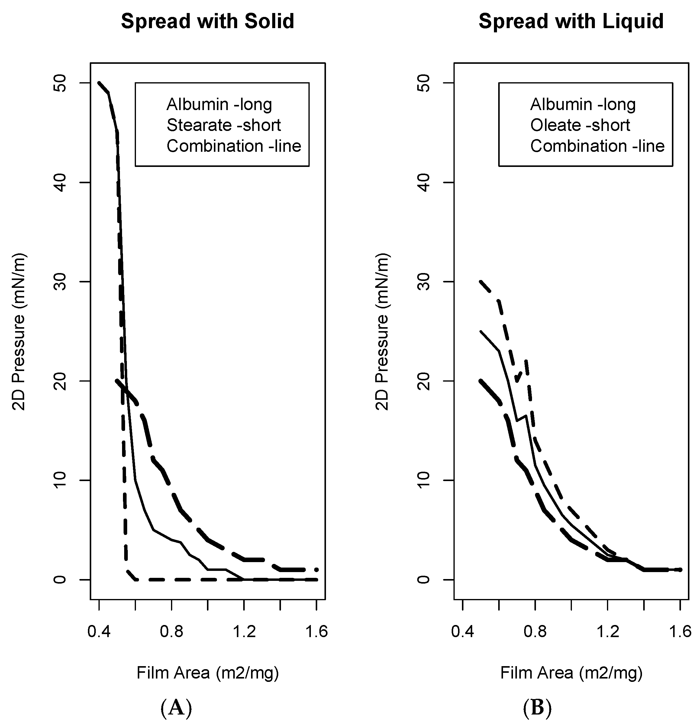
8. Spreading Exercises

Our original organoaerosol papers and related publications [30,31,32,33,37] dealt only with the Langmuir isotherm. We determined here that this initial choice works well to represent laboratory profiles of the sigmoidal protein π [95]. However, the lipid proxy constitutes an instance of 2D solidification in π-A space—surface pressure remains at zero until the film area is reduced beyond a sharp threshold, at which point π rapidly increases. To resolve this issue, in the equations in Appendix A we introduce what will be referred to as a “power-Langmuir” form, in which the classic “S” shape is adjustable. The main motivation is to handle stearate (lipids), although there are additional benefits in dealing with the protein multiplex (ring formation, bunching and balling at the interface). In Equations (A10) and (A11) (Appendix A), the dominant terms are raised to the nth degree. The choice of exponents loosens or tightens the standard sigmoidal shape associated with the Langmuir isotherm allowing for the steep 2D solid behavior to be captured. The function we propose is similar to a saturating Freundlich isotherm. Our π have been designed for near-agreement with laboratory data [63,94,95]. We also numerically compute the elasticity modulus (ε)—the derivative against fractional surfactant area change [17]. Finally, a surface phase state (2D solid, liquid, gas) is assigned based on the shape/pattern [5,18]. We also supplement with the more recent interpretations of Frew et al. [19]. This procedure allows us to check against the magnitude, form, and planar phase of real oceanographic π-A.

Results of these global exercises are summarized in

Table 4. Upper lines—surface pressure estimates based on collected results from Table 3 and computed per the Appendix A, with a selection of data spanning several decades for comparison. In the center of the table, local elastic modulus results are offered. Finally, in the lower lines, model and data π-A experiments are reported in the form of phases. The background (bloom) nonparenthetical (parenthetical) convention is retained. Letters g, l and s stand for 2D gas, liquid and solid.

Surfactomes	Coastal (Mid-Lat)	Coastal (Low-Lat)	Polar	Westerly	Equator (East)	Equator (West)	Gyre
Surface Pressure and Modulus, units mN/m both Cases
π (Appendix)	2.4 (9.4)	2.9 (6.7)	0.65 (50)	0.65 (2.9)	6.5	1.8	0.65
π (data)	0.3 (23)	0.1 (10)		0.1 (5)			0.1–1
ε (local)	6.6 (25)	8.0 (18.1)	1.6 (175)	1.5 (8.2)	10	4.9	1.6
2D Phase
Model	g (l-s)	g (g)	g (s)	g (l)	s	g	g
Data	g-l (l)	g-l (l)			l-s

. Ambient π and phase state identifications are drawn from a variety of the above references and more [2,3,4,5,6,7,9,17,18,85,120,121,122,123,124]. Ratios of surfactome-level protein to lipid concentration were fed into our Appendix A π-A-modulus code. Fast equilibration is assumed, to guarantee close tracking of reference concentrations just below the Gibbs plane. The interfacial composition and solute levels are then tightened together in a computational Langmuir-Blodgett (trough) experiment to give π(A). Typical curves attributable to the open ocean are reproduced. However, in laboratory work material is often lost to redissolution, stacking, or the extraction medium [2,3,4,5,63]. At local concentrations for the biomacromolecules, we compare with several decades of film pressure measurements. Although data remain scarce, the proposed patterns and trends are encouraging. Surface pressures tend to increase in reverse order across the Table 1 range—moving from gyres toward neighboring equatorial ecosystems or boundary current extensions. Given the uncertainties, polar and coastal values could cross the 0.3–3 mN/m band on a seasonal basis. Modulus translated into 2D phase information gives us relationships along the g-l-s spectrum. Overall, our fourth table allows us to begin addressing quantitatively the two key questions proposed at the top of the paper. Even based on a regional view, biogeographic dependencies are likely for the tension difference, and there is a potential for crossing of the geophysical fluidic π range (0.3–3 mN/m).

9. Maps and Sensitivity

Protein and lipid distributions from the Ogunro et al. computation [33] were drawn upon for the initial surface tension mapping attempts. The O15 values are central among Table 3 model outputs. Background biogeochemistry in this work traces to early marine methane cycle simulations [125] and the BEC ecodynamics code [41,42]. Ogunro and company proposed source-removal functions closely matching our Longhurst biogeographic steady state, but phytoplankton and zooplankton levels were extracted directly from model history files. They may be viewed as dynamic and the entire procedure as semi-dynamic. Our Appendix A surface pressure algorithm was transferred into an offline data package so that it could operate on upper mixed layer concentrations to produce π patterns suitable for analysis. We now discuss the fully-mapped results referring to central months of the seasons—primarily February and August, corresponding to winter and summer in the two hemispheres. All results represent years surrounding the new millennium [41,125]. Major sensitivity tests are also described in this section.

The original Ogunro mechanism is adopted as our global baseline, and in Figure 1 we scan the Northern Hemispheric winter then summer results (opposite for the Southern Ocean). A logarithmic color bar is arranged so that the suggested indicator band 0.3–3 mN/m is central and can easily be located (−0.5 to 0.5 in log space). The values correspond to green and yellow tones and they apply to all images. An upper limiting pressure of 100 was chosen as a round decadal value bracketing the large lipid π maximum recorded for stearic acid [94]. It is clear in the first panel that marine surface tension probably does possess a measurable biogeography. Hence, question 1 from the introduction has already been answered in the affirmative. If our proxy set is realistic, it should be possible for the shipboard chemist to identify 2D pressure lows in many areas. Moreover, solid-driven peaks may be observable in high-latitude summer (Antarctic coast, then the Sea of Okhotsk and Bering in our six-monthly plots). In the North Pacific and Atlantic, a band of low π can be observed, from the subpolar regime across middle latitudes and into the subtropics, moving generally east to west. In autumn, it is bracketed by lingering activity in the respective western boundary current extensions and along equatorial upwellings.

In Figure 1, a marine geography of tension is apparent in broad outline, driven by biology, but more fundamentally by surfactant behavior of specific detrital macromolecules. At middle latitudes, the estimated surface pressure values fall to a minimum (log ≈ 0) in the remote central ocean. Blue to purple tones are largely absent from this initial color distribution. The geophysical fluid dynamic effects defined in Table 1 would be enhanced if there were obvious regional or seasonal transitions across the 0.3–3 ribbon recommended earlier as a reference.

Mixed-layer biogeochemistry models underlying Table 3 and Table 4 were consulted first as a group because measurements of the macromolecular classes are so disperse [33,37,109]. There could be no opportunity for space filling or interpolation from limited, province-scale averages. However, the reader should note from the tables that both our protein levels and the π driven by them could be biased high. Meanwhile, computed lipid values may, by contrast, fall on the low side of ambient. We remark that no global model can currently resolve rich generation occurring coastally then transported outward [113,125]. In a second global simulation we, therefore, lowered (raised) the protein (lipid) distributions (respectively) by factors of three. This was accomplished by adjusting the removal time constants in both cases. February and August results are shown as our Figure 2. Well-characterized features emerge in the pre-defined 0.3–3 mN/m regime, and solidification (2D crystallization) is pervasive at high latitudes.

Several crucial properties of the tension distribution system are amplified in Figure 2, and they deserve specific comment. We focus first on a relative absence of Northern Hemispheric surfactants at middle latitudes in the August plot. The bow-tie shaped 2D pressure minimum running from California over Hawaii to the Philippines may be attributed to restricted gyre and warm pool biology, bordered on either side by nutrient upwelling regions—the boundary current extension, plus equatorial divergence. A western boundary extension bloom remains imprinted upon the interface since succession carries the macromolecules through into summer. The central Pacific path of the minima falls precisely in an area where reanalyses indicate that CMIP class climate models may be overestimating wind speeds (Figure A1 in [84]). The ocean surface is, perhaps, rougher than expected here, because Table 1 surfactant influence is not considered within the CMIP models. Brunke and company have demonstrated [67,93] that attempts to include ocean ripples in turbulent flux parameterizations tend to overestimate momentum transfer. This may occur because they are typically formulated from a meteorological perspective. The absence of wave dampening resulting from marine organic chemistry is, therefore, a possible explanation. It is worth recalling that aerodynamic drag studies are most often conducted either in the coastal context, at middle latitudes, or else in seasonable weather [92,126,127]. These are conditions under which our arguments and figures suggest that regional dampening should be effective. Some versions of the tension biogeography imply that flux measurement calculations should factor in film geochemistry.

Yellow-to-red tones in the bottom panel of Figure 2 suggest a “crystallization” of the regional scale microfilm over the entire Arctic Ocean. This is due to the small augmentation in average lipid concentrations (stearate), but cannot currently be verified. Potential implications include unexpected microlayer influence on all major effects under consideration here, from gas-bubble-aerosol mass transfer, whether at the pack edge or along leads, up to general wind fields of the ice domain. The 2D condensation result penetrates far beneath the perimeter of summer ice coverage, tracking primary production [42,125]. Even a minor underestimation of generalized surfactant levels could have major implications for high-latitude climate. Closely related (detrital) biomacromolecules are also generated independently inside of sea ice, by the resident sympagic algae. At extreme temperatures and salinities characterizing the interior of the pack, organics tend to coalesce, gel, and coat pore spaces and their interconnecting channels [128]. This could alter brine drainage rates, nutrient resupply chains and, possibly, the average regional-scale freezing point [129]. Surface physicochemistry again offers the right theoretical framework. Equations will strongly resemble room temperature film thermodynamics as outlined in Appendix A [130].

Figure 2 directly addresses the second issue raised at the top of the text, but without offering a definitive answer. It seems possible that the specific surrogate pairing, of albumin with stearic acid, is giving us a fair representation of the relative regional surface tension variation. The π maps presented here would then be consistent with (1) the breadth of the aerosol gas precursor and primary particle effects implied in the first table; (2) unexpected roughness across broad sectors of the middle latitude open ocean; (3) overestimation of the momentum transfer in turbulent flux parameterizations lacking film chemistry; and even (4) 2D microfilm collapse over large areas at high latitudes. However, data remain lacking to assess these options in depth. For the moment, all that can be done is to provide guidance for renewed laboratory or seagoing experimental work.

We believe, due to improved agreement with the limited datasets for protein-like material and for π (Table 3 and Table 4), that the albumin lowered by three (Alb/3) calculation may be our most realistic product. For example, across the well-studied Westerly regime, an average of simulated protein significantly exceeds the measurement base regardless of season, while resulting π are also sometimes excessive. For the sake of completeness, we include the associated May and November plots as Figure 3. In this figure lipid blooms have been moderated by a return to baseline, but the bow-tie shaped depression is emphasized in autumn as it runs across the northern basin Pacific. Alb/3 is finally taken as a sub-baseline for two further maps of interest—lipid, then protein, influence switched off. With the stearate contribution removed, no zones of high surface pressure remain (all are below 10 mN/m in Figure 4). This suggests that some form of 2D solid (lipid) will be a necessary component in successful parameterizations since steepness is observed [2,3,4,5,63]. Only under severe reduction of our protein proxy (Figure 5), does the central basin surface pressure fall below tenths mN/m. Historical droplet determinations demonstrate that such values should often be detectable [2,81]. Results presented by Figure 4 and Figure 5 indicate that the surrogate combination in Appendix A is effective, as predicted by many earlier surfactant chemical groups.

Global tests for which results will not be shown include (2D) liquefaction of the lipid proxy by substituting oleic acid profiles [5,63], swapping-in of casein or lysozyme in place of the albumin gas-liquid [95], alterations to the half-saturation reference points and, finally, sensitivities to other equation of state parameters as outlined in Appendix A (

Table A1. Parameter settings drawn from the physical chemical surfactant literature to describe the interfacial behaviors of the proxy compounds. The following are startup information sources: albumin data from Graham and Philips [95], plus stearic acid from Christodoulou and Rosano [94]. CR do not actually quote bulk liquid concentrations, but these have been estimated from Ter Minassian-Saraga [173] and Brzozowska et al. [174]. Values are inserted into the appendix equations to generate the π-A plots shown in Figure A1, π-ε as in the main text tables, and any global maps presented.

Surrogate	Reference Concentrations 1/2 Max, all μM Carbon		Maxima (Γ mg/m2, π as mN/m)		Exponents Values for n
	Excess	2D Pressure	Excess	2D Pressure	Excess	2D Pressure
Protein (Albumin)	10	30	2	20	0.5	1
Lipid (Stearate)	0.5	2	2.5	50	1	8

). Results of the previous figures are not contradicted and, in fact, they are largely continually confirmed by further exercises. Overall, the marine macromolecules and polymers should describe a distinct biogeography of surface tension, along with its absolute difference (2D pressure), while intra-basin and seasonal variations may often cross the 0.3–3 mN/m reference contour band. The latter transition, per Table 1, implies a fluid geographic relationship to both aerosol sources and boundary layer physics. Patterns may be decipherable through the phase plane equation of state approach.

10. Uncertainties

Some errors inherent in the above development are parametric, and were explored in the figure set. Examples include macromolecular release rates and surrogate choices. Other potential uncertainties should be termed “structural”, and they are described independently here. To participate in the interfacial energetics, polymers must undergo a full life cycle of transformations over hours to weeks, including the following steps: biological release, which may be targeted rather than detrital; chemical reactions in an oxidizing and light rich medium (the mixed layer); transport toward the atmospheric boundary through the spectrum of turbulent eddies; equilibration along the wave system; and, finally, surfactant function within the Gibbs plane. An objective of the present work was to provide evidence that the latter constitutes its own complex biogeochemical medium. This local, 2D phase experiences continual compression and dilation by the wave field, interactions with constituents of the bulk atmospheric gas phase sometimes in bubble form, and more. We have assumed a rapidly-stirred upper ocean; uniform heteropolycondensate evolution among the DOC, except for a few adjustable exponential time constants, instant stabilization into the surfactant medium, fixed moderate thermochemical temperatures, which are actually confined to the laboratory or corresponding middle latitudes, undisturbed occupation of an idealized pristine monolayer, experiment-like responses constrained to be nonstacking and nonhysteretic, and a complete lack of 2D-internal removal or reactive processes.

Potential model structural omissions are so numerous that we hesitate to list them further except in bullet form. Details remaining for investigation involve:

• Exudation mechanisms which could be “intentional”, e.g., the siderophores [131,132];
• Water column processing into alternate bulk phases, such as gels [133,134,135,136,137];
• Vertical gradients and alternate transport via bubble impaction [138,139,140,141];
• Finite timescales for attachment/detachment—surface kinetics [1,29,46,62,77,80,142];
• Mixing state within the monolayer as a perturbation to ideality [36,38,142,143,144];
• Microbiology perhaps partitioned by analogy with white caps [2,74,75,145,146,147];
• Effects on the surfactant equilibria:

  ◦

  The Van’t Hoff isochore (temperature) [38,95,148]

  ◦

  Salt Effects [94,95,149]

• Acid-base reactions within and just below the monolayer (2D pH) [77,94,149,150];
• Multiplexing into layers, rings, balls, etc., with hysteresis [31,36,95,135,142];
• Accumulation in sea foam with indeterminate residence time [28,151,152,153,154]; and
• Interaction with atmospheric tracers, such as oxidants and metals [76,103,155,156].

We make no attempt to quantify such biases at this early stage. Any one of them could arguably inject a factor of three flexibility into the logic, and some would operate in two directions. We have already used a rounded half-decadal value several times just in carrying out our plotting procedures. Since numerous uncertainties exist, both cancellation and accumulation are statistical possibilities. It may be that either the sum of uncertainty disappears, or else that it is much greater than suspected. Measurement constraints are few, but real (earlier tables), and we exploit them as fully as possible. Effectively, we claim that traditional fluid drop methods, skim sampling, and experimental π-A curves are all consistent with our results. Therefore, they support our hypotheses.

Our position, as might be imagined, is that parameter ranges explored in the figures already point to major opportunities for the international communities of atmospheric, environmental, and surfactant chemists. Improved geographic coverage is needed for all measurements implied—the families of lipids, polymers, hybrids, and degradation products among compounds in the sea. In addition to their concentration gradients (provincial and vertical), film densities, specific physical behaviors during surface activity, the presence in the aerosol, and even the possibility of recycling from the atmosphere, should all be investigated. Molecular dynamics and statistical mechanics modeling may be called for [143,144]. There is much to be learned from traditional marine aerosol research, which has long focused on aqueous/salt/organic phases and surface relationships critical to CCN number and cloud brightness [102,103,157].

The required research could be organized geographically via surfactome principles drawn from Table 3 and Table 4. Automated sensors and their respective platforms could determine the mix of techniques. Many groups have demonstrated that centimeter-scale waves or, conversely, the slicks left behind by damping, are detectable by robotic instruments shipboard, airborne, or from space [8,9,19,64]. Remotely-sensed white cap distributions and residence times have been used to estimate the air entrapment caused by wave-breaking events. Data on the entrained air volumes feed into bubble plume energetics calculations. Tank experiments suggest, however, that surfactant identities impose a large mode of uncertainty [28,151,158]. A spread in white cap data may conceal information on the chemical and biological geography of marine films.

Some uncertainties characterized in our bullet list reinforce preexisting needs. For example, proteins and lipids comprise a poorly understood portion of the total DOC at any given location (Table 3). Marine colloids ultimately become active carbon carriers [75,134,135,136] formed from the remaining macromolecular mass—the 20% of spillage which dissolves as polysaccharide, and fuels the gel phase. Gel particles are buoyant and, therefore, advect vertically into a dead end at the microlayer. There they occupy an undetermined fraction of local microarea, acting as a pseudo-polymeric embedded phase. If dissolved proteins and lipids adsorb to the chained sugars, a surfactant pathway additional to the expected bubble sweep has been identified [37,141].

Further instances can readily be cited—dust iron deposition as redox chemistry, or inputs by short-lived bulk gas radicals [76,155]. Photoreduction in mineral aerosol coatings can solubilize trace metals during long-range atmospheric transport [155,156], but organic ligands determine equilibrium and persistence. One of us (NM) is now conducting laboratory dust iron research into the strength of far upper ocean chelation. That which sets in quickly as mineral particles enter the sea turns out to be crucial to reoxidation rates and bioavailability. Strong multidentate ligands must be numbered among the macromolecules considered here [110] and the process of monolayer penetration-acquisition appears not to have been accounted by iron cycle specialists. We have remarked elsewhere that our macromolecules have equivalents inside polar ice, generated and processed in a very similar manner. A significant fraction of this organic mass will be surface active at the bulk solid boundary of brine channels, where the average freezing point is subject to alteration [128,129,130].

11. Summary and Discussion

Drawing on Langmuir surfactant concepts lately applied to marine organic aerosol emissions ([30,31,32,33]—the developing OCEANFILMS code), we extend toward a complete physicochemistry of global interfacial mass and energy transfer. Our hope is to illuminate not only marine gas and particle release, but also organochemical aspects of momentum and heat flux (Section 2, Section 3 and Section 4, Table 1). In all cases a key quantity is the surface tension, here represented by its difference relative to the baseline, known as the two-dimensional pressure π ([1,2,3,4,5,36,37,38], Section 3 and Section 4, plus Appendix A). The in situ value is dictated by macromolecular surfactant composition, so that Gibbs planar thermodynamics have been applied to the entire film system dividing ocean from atmosphere. Theoretical connections are facilitated by a combination of ecodynamics, nutrient-carbon cycle, and macromolecular surface chemistry modeling, conducted at the top of the mixed layer (Section 5, Section 6 and Section 7). All this takes place at a planetary scale, so that influences can be assessed upon coupled ocean-atmosphere biogeocycling, atmospheric and aerosol chemistry, and regional climate. We seek to organize the macromolecular surfactant issues geographically, by searching for underlying patterns at the biome to basin level (Section 8 and Section 9). Our study is framed by two questions—can π be mapped adequately, and usefully? Both historical and modern sources are consulted for the marine interfacial, organic, and surface chemical information required (Section 2, Section 3, Section 4, Section 5 and Section 6). We supplement with state-of-the-art biogeochemical systems modeling and graphical analysis (Section 7, Section 8 and Section 9). Specific biogeographies are assigned to the dominant macromolecular classes and their tension properties. Both tabled and plotted results show that the answers to our fundamental questions lie in the affirmative—π can now be computed and presented such that thresholds for flux alteration are comprehensible—piston velocities, bubble film breakage, sea spray number, primary organic particulates, centimeter scale (capillary) wave damping, the drag coefficient, and several other aerosol or energetic quantities are all influenced. The results we obtain are tentative, but robust. A potential for regional- to basin-scale effects on multiple geophysical transport modes cannot be excluded (Section 9).

Along the way we have called upon standard (surface chemistry) text materials, long-standing literature to define less familiar (Gibbsian) planar phase states within the film (Section 3, Section 4 and Section 8, and Appendix A), community knowledge of detailed macromolecular composition for the marine dissolved organic matter—with special emphasis on functionalities and amphiphilicities (Section 5), classic chemical oceanographic surfactant research providing a recommended and tractable proxy set (Section 6), global ecodynamic systems modeling performed at several levels, yielding similar, self-reinforcing distributions (Section 7), numerous marine (2D or surface) pressure-area diagrams (Section 8 plus Appendix A) and, finally, global maps demonstrating that surface tension gradients driven by the organics should be real and detectable (Section 9). We conclude with an enumeration for the large number of uncertainties involved. Simultaneously, however, we show that some of these can be turned to the community’s advantage—the unknowns motivate further research (Section 10).

In an historical analysis, Cox and company [46] have recreated nineteenth century wave calming experiments, conducted using petroleum liquids and fish oil. The former substances (pure hydrocarbons) gather and bead at the atmospheric interface having little effect, while the latter are 2D gases (elastic [16,17,18,19,36], Appendix A). The authors offer a heuristic, but quantitatively grounded, explanation of breaker suppression at the kilometer-scale. Their claim is that it occurs through the cascade of effects outlined in our background material, propagating from the atmospheric turbulent field into, and through, upper ocean eddy spectra. Here, we have shown that the logic can also be derived from adsorption chemistry fundamental to sea salt aerosol and primary organic emissions ([30,31,32,33], OCEANFILMS). We track phytoplanktonic detritus from its inception in regional food webs through individual biomacromolecular identities into the Gibbs phase plane, where critical comments can be made regarding mass and energy injections. It seems plausible that knowledge of surfactant and biopolymer chemistry at the global interface implies enhanced control over aerosol, wind, wave, current, and energy systems. Our work reinforces the prospect that there may exist closely inter-related, basin-scale biological feedbacks onto a long list of planetary transfer types—including gas, salt, primary and secondary organics, heat, momentum, carbon, radiation, and water vapor fluxes [2,18,20,22,46,83,159]. All of this is previewed in the present work in an offline manner, but it has become possible only given contemporary, state-of-the-art global model and mapping techniques. We believe this is even more reason to attempt a full integration, for understanding of the flux-filtering 2D equilibria at stake. Phase plane energetics will fit neatly into the primary organic emissions package, OCEANFILMS, which ingests macromolecular concentrations and returns film coverage [30,31].

Our research distills to a parameterization for the planar equation of state (EOS, Appendix A), but we have applied it around the entire planetary ocean surface. This implies that there will be many inadequacies (Section 10), but the strategy is simple to test. Textbook expositions of the EOS concept begin from bulk aqueous media, making connections to the tangential forces through 2D densities and on to chemistry [5,38,130]. Surfactant specialists have experimented with such systems regularly over the decades [5,36,77,94,95,103]. Occasionally, dynamic and statistical computational methods are applied to this type of problem [143,144,160]. The approach outlined in the Appendix A is almost purely empirical, but expect it to fall back in these rigorous directions. A guess is that our “power Langmuir” equation must be derivable from first principles. Similar forms have been found to represent low kinetic reaction molecularities on catalytic surfaces. We, therefore, conclude by proposing computational experiments over Table 3 and Table 4 surfactomes as a starting point for introducing detail. First-order concepts will be incorporated into our own OCEANFILMS parameterization, which is already running in a global systems mode [30,31,32].

References

1. Jarvis, N. Adsorption of surface-active material at the sea-air interface. Limnol. Oceanogr. 1967, 12, 213–221. [Google Scholar] [CrossRef] [Green Version]
2. Liss, P. Chemistry of the sea surface microlayer. In Chemical Oceanography; Riley, J., Skirrow, G., Eds.; Academic Press: New York, NY, USA, 1975; Volume 2. [Google Scholar]
3. Barger, W.; Daniel, W.; Garrett, W. Surface chemical properties of banded sea slicks. Deep Sea Res. Oceanogr. Abstr. 1974, 21, 83–89. [Google Scholar] [CrossRef]
4. Barger, W.; Garrett, W. Surface active organic material in air over the Mediterranean and the Eastern Equatorial Pacific. J. Geophys. Res. 1976, 81, 3151–3163. [Google Scholar] [CrossRef]
5. Barger, W.; Means, J. Clues to the structure of marine organic material from the study of physical properties of surface films. In Marine and Estuarine Geochemistry; Sigleo, A., Haitori, A., Eds.; Lewis Publishers: Chelsea, MI, USA, 1985. [Google Scholar]
6. Goldman, J.; Dennett, M.; Frew, N. Surfactant effects on air-sea exchange under turbulent conditions. Deep Sea Res. 1988, 35, 1953–1970. [Google Scholar] [CrossRef]
7. Ermakov, S.; Salashin, S.; Panchenko, A. Film slicks on the sea surface and some mechanisms of their formation. Dyn. Atmos. Oceans 1992, 16, 279–304. [Google Scholar] [CrossRef]
8. Peltzer, R.; Griffin, O.; Barger, W.; Kaiser, J. High resolution measurement of surface active film redistribution in ship wakes. J. Geophys. Res. 1992, 97, 5231–5252. [Google Scholar] [CrossRef]
9. Wei, Y.; Wu, J. In situ measurements of surface tension wave damping and wind properties modified by natural films. J. Geophys. Res. 1992, 97, 5307–5313. [Google Scholar] [CrossRef]
10. Riley, W.; Skirrow, G. Chemical Oceanography; Academic Press: New York, NY, USA, 1975; Volume 1 & 2. [Google Scholar]
11. Herr, F.; Williams, J. Role of Surfactant Films on the Interfacial Properties of the Sea Surface; Office of Naval Research: London, UK, 1986. [Google Scholar]
12. Liss, P.; Duce, R. The Sea Surface and Global Change; Cambridge University Press: Cambridge, UK, 1997. [Google Scholar]
13. Jones, I.; Toba, Y. Wind Stress over the Ocean; Cambridge University Press: Cambridge, UK, 2001. [Google Scholar]
14. Lewis, E.; Schwartz, S. Sea Salt Aerosol Production; American Geophysical Union: Washington, DC, USA, 2004. [Google Scholar]
15. Gade, M.; Huhnerfuss, H.; Korenowski, G. Marine Surface Films; Springer: Berlin, Germany, 2006. [Google Scholar]
16. Frew, N.; Nelson, R. Isolation of marine microlayer film surfactants for ex situ study of their physical and chemical properties. J. Geophys. Res. 1992, 97, 5281–5290. [Google Scholar] [CrossRef]
17. Bock, E.; Frew, N. Static and dynamic response of natural ocean surface films to compression and dilation: Laboratory and field observations. J. Geophys. Res. 1993, 98, 14599–14617. [Google Scholar] [CrossRef]
18. Frew, N. The role of organic films in air-sea gas exchange. In The Sea Surface and Global Change; Liss, P., Duce, R., Eds.; Cambridge University Press: Cambridge, UK, 1997. [Google Scholar]
19. Frew, N.; Nelson, R.; Johnson, C. Correlation studies of mass spectral patterns and elasticity of sea-slick materials. In Marine Surface Films; Gade, M., Huhnerfuss, H., Korenowski, G., Eds.; Springer: Berlin, Germany, 2006. [Google Scholar]
20. Asher, W. The sea-surface microlayer and its effect on global air-sea gas transfer. In The Sea Surface and Global Change; Liss, P., Duce, R., Eds.; Cambridge University Press: Cambridge, UK, 1997. [Google Scholar]
21. Tsai, W.; Liu, K. An assessment of the effect of sea surface surfactant on atmosphere-ocean CO2 flux. J. Geophys. Res. 2003, 108. [Google Scholar] [CrossRef]
22. Ito, A.; Kawamiya, M. Potential impact of ocean ecosystem changes due to global warming on marine organic aerosols. Glob. Biogeochem. Cycles 2010, 24. [Google Scholar] [CrossRef]
23. Vignati, E.; Facchini, M.; Scannel, C.; Ceburnis, D.; Sciare, J.; Kanakidou, M.; Dentener, F.; O’Dowd, C. Global scale emission and distribution of sea-spray aerosol: Sea-salt and organic enrichment. Atmos. Environ. 2010, 44, 610–677. [Google Scholar] [CrossRef]
24. Meskhidze, N.; Xu, J.; Gantt, B.; Nenes, Y.; Ghan, S.; Liu, X.; Easter, R.; Zaveri, R. Global contribution and climate forcing of marine organic aerosol 1: Model improvements and evaluation. Atmos. Chem. Phys. 2011, 11, 11689–11705. [Google Scholar] [CrossRef] [Green Version]
25. Detwiler, A.; Blanchard, D. Aging and bursting bubbles in trace-contaminated water. Chem. Eng. Sci. 1978, 33, 9–13. [Google Scholar] [CrossRef]
26. Gagosian, R.; Zafiriou, O.; Peltzer, E.; Alford, J. Lipids in aerosols from the tropical North Pacific: Temporal variability. J. Geophys. Res. 1982, 87, 11133–11144. [Google Scholar] [CrossRef]
27. O’Dowd, C.; Facchini, M.; Cavalli, F.; Ceburnis, D.; Mircea, M.; Decesari, S.; Fuzzi, S.; Putaud, J. Biogenically driven organic contribution to marine aerosol. Nature 2004, 431, 676–681. [Google Scholar] [CrossRef] [PubMed]
28. Modini, R.; Russell, L.; Deane, G.; Stokes, M. Effect of soluble surfactant on bubble persistence and bubble produced aerosol particles. J. Geophys. Res. 2013, 118. [Google Scholar] [CrossRef]
29. Alpert, P.; Kilthau, W.; Bothe, D.; Radway, J.; Aller, J.; Knopf, D. The influence of marine microbial activities on aerosol production: A laboratory mesocosm study. J. Geophys. Res. 2015, 120. [Google Scholar] [CrossRef]
30. Burrows, S.; Ogunro, O.; Frossard, A.; Russell, L.; Rasch, P.; Elliott, S. A physically based framework for modeling the organic fractionation of sea spray aerosol from bubble film Langmuir equilibria. Atmos. Chem. Phys. 2014, 14, 13601–13629. [Google Scholar] [CrossRef]
31. Burrows, S.; Gobrogge, E.; Fu, L.; Link, K.; Elliott, S.; Rasch, P.; Wang, H.; Walker, R. OCEANFILMS-2: Representing co-adsorption of marine surfactants and soluble polysaccharides improves simulation of marine aerosol chemistry. Geophys. Res. Lett. 2016, 43, 8306–8313. [Google Scholar] [CrossRef]
32. McCoy, D.; Burrows, S.; Wood, R.; Grosvenor, D.; Elliott, S.; Ma, P.; Rasch, P.; Hartmann, D. Natural aerosols explain seasonal and spatial patterns of Southern Ocean cloud albedo. Sci. Adv. 2015. [Google Scholar] [CrossRef] [PubMed]
33. Ogunro, O.; Burrows, S.; Elliott, S.; Frossard, A.; Hoffman, F.; Letscher, R.; Moore, J.; Russell, L.; Wang, S.; Wingenter, O. Global distribution and surface activity of macromolecules in offline simulations of marine organic chemistry. Biogeochemistry 2015, 126, 25–56. [Google Scholar] [CrossRef] [Green Version]
34. Szyszkowski, B. Experimentelle Studien uber kapillare Eigenschaften der wassrigen Losungen von Fettsauren. Z. Phys. Chem. 1908, 64, 385–414. [Google Scholar] [CrossRef]
35. Langmuir, I. The constitution and fundamental properties of solids and liquids II. Liquids. J. Am. Soc. 1917, 39, 1848–1906. [Google Scholar] [CrossRef]
36. Adamson, A. Physical Chemistry of Surfaces; Interscience: Easton, PA, USA, 1960. [Google Scholar]
37. Elliott, S.; Burrows, S.; Deal, C.; Liu, X.; Long, M.; Ogunro, O.; Russell, L.; Wingenter, O. Prospects for simulating macromolecular surfactant chemistry at the ocean-atmosphere boundary. Environ. Res. Lett. 2014, 9, 064012. [Google Scholar] [CrossRef]
38. Davies, J.; Rideal, E. Interfacial Phenomena; Academic Press: London, UK, 1963. [Google Scholar]
39. Longhurst, A. Ecological Geography of the Sea; Academic Press: San Diego, CA, USA, 1998. [Google Scholar]
40. Longhurst, A. Ecological Geography of the Sea; Elsevier: San Diego, CA, USA, 2007. [Google Scholar]
41. Moore, J.; Doney, S.; Kleypas, J.; Glover, D.; Fung, I. An intermediate complexity marine ecosystem model for the global domain. Deep-Sea Res. II 2002, 49, 403–462. [Google Scholar] [CrossRef]
42. Moore, J.; Doney, S.; Lindsay, K. Upper ocean ecosystem dynamics and iron cycling in a global three dimensional model. Glob. Biogeochem. Cycles 2004, 18, 18. [Google Scholar] [CrossRef]
43. Letscher, R.; Moore, J. Preferential remineralization of dissolved organic phosphorus and non-Redfield DOM dynamics in the global ocean. Global Biogeochem. Cycles 2015, 29, 325–340. [Google Scholar] [CrossRef]
44. Franklin, B. Of the stilling of waves by means of oils. Philos. Trans. R. Soc. Lond. B 1774, 64, 445–460. [Google Scholar] [CrossRef]
45. Wang, D.; Steiglitz, H.; Marden, J.; Tamm, L. Philadelphia’s favorite son was a membrane biophysicist. Biophys. J. 2013, 104, 287–291. [Google Scholar] [CrossRef] [PubMed]
46. Cox, C.; Zhang, X.; Duda, T. Suppressing breakers with polar oil films: Using an epic sea rescue to model wave energy budgets. Geophys. Res. Lett. 2016, 44. [Google Scholar] [CrossRef]
47. Sverdrup, H.; Johnson, M.; Fleming, R. The Oceans: Their Physics, Chemistry and General Biology; Prentice-Hall: New York, NY, USA, 1942. [Google Scholar]
48. Cox, C.; Munk, W. Statistics of the sea surface derived from sun glitter. J. Mar. Res. 1954, 16, 231–240. [Google Scholar]
49. Blanchard, D. The electrification of the atmosphere by particles from bubbles in the sea. Prog. Oceanogr. 1963, 1, 73–202. [Google Scholar] [CrossRef]
50. Davies, J. The effects of surface films in damping eddies at a free surface of a turbulent liquid. Proc. R. Soc. Lond. A 1966, 290, 515–526. [Google Scholar] [CrossRef]
51. Jarvis, N. The effect of monomolecular films on surface temperature and convective motion at the water/air interface. J. Colloid Sci. 1962, 17, 512–522. [Google Scholar] [CrossRef]
52. Garrett, W. The influence of monomolecular surface films on the production of condensation nucleii from bubbed sea water. J. Geophys. Res. 1968, 73, 5145–5150. [Google Scholar] [CrossRef]
53. Paterson, M.; Spillane, K. Surface films and the production of sea salt aerosol. Q. J. R. Meterol. Soc. 1969, 95, 526–534. [Google Scholar] [CrossRef]
54. Hoffman, E.; Duce, R. Factors influencing the organic carbon content of marine aerosols: A laboratory study. J. Geophys. Res. 1976, 81, 3667–3670. [Google Scholar] [CrossRef]
55. Liss, P.; Slater, P. Flux of gases across the air-sea interface. Nature 1974, 247, 181–184. [Google Scholar] [CrossRef]
56. Levich, V. Physicochemical Hydrodynamics; Prentice Hall: Englewood Cliffs, NJ, USA, 1962. [Google Scholar]
57. Lucassen-Reynders, E.; Lucassen, J. Properties of capillary waves. Adv. Colloid Interface Sci. 1969, 2, 347–395. [Google Scholar] [CrossRef]
58. Jenkinson, I. Oceanographic implications of non-Newtonian properties found in phytoplankton cultures. Nature 1986, 323, 435–437. [Google Scholar] [CrossRef]
59. Ermakov, S.; Zujkova, A.; Panchenko, A.; Salashin, S.; Talipova, T.; Titov, V. Surface film effects of short wind waves. Dyn. Atmos. Oceans 1986, 10, 31–50. [Google Scholar] [CrossRef]
60. Piexoto, J.; Oort, A. Physics of Climate; Springer: Berlin, Germany, 1992. [Google Scholar]
61. Dysthe, K. On surface renewal and sea slicks. In Marine Surface Films; Gade, M., Huhnerfuss, H., Korenowski, G., Eds.; Springer: Berlin, Germany, 2006. [Google Scholar]
62. Garrett, W. Organic chemical composition of the ocean surface. Deep-Sea Res. 1967, 14, 221–227. [Google Scholar] [CrossRef]
63. Jarvis, N.; Garrett, W.; Scheiman, M.; Timmons, C. Surface chemical characterization of surface active material in seawater. Limnol. Oceanogr. 1967, 12, 88–96. [Google Scholar] [CrossRef]
64. Wu, J. Suppression of ripples by surfactant: Spectral effects deduced from sun glitter, wave staff and microwave measurements. J. Phys. Oceanogr. 1989, 19, 238–245. [Google Scholar] [CrossRef]
65. Mitsuyasu, H.; Bock, E. The influence of surface tension. In Wind Stress over the Ocean; Jones, I., Toba, Y., Eds.; Cambridge University Press: Cambridge, UK, 2001. [Google Scholar]
66. Brunke, M.; Zeng, X.; Anderson, S. Uncertainties in sea surface turbulent flux algorithms and data. J. Geophys. Res. 2002, 107. [Google Scholar] [CrossRef]
67. Brunke, M.; Zeng, X.; Misra, V.; Beljaars, A. Integration of a prognostic sea surface skin temperature scheme into weather and climate models. J. Geophys. Res. 2008, 113. [Google Scholar] [CrossRef] [Green Version]
68. Lodziana, Z.; Topsoe, N.; Norskov, J. A negative surface energy for alumina. Nat. Mater. 2004, 3, 289–293. [Google Scholar] [CrossRef] [PubMed]
69. Tuckermann, R. Surface tension of aqueous solutions of water-soluble organic and inorganic compounds. Atmos. Environ. 2007, 41, 6265–6275. [Google Scholar] [CrossRef]
70. Ulabanathan, V.; Fainerman, V.; Gochev, G.; Aksenenko, E.; Gunes, D.; Gehin-Delval, C.; Miller, R. Evidence of negative surface pressure induced by beta lactoglobulin and casein at the water/air interface. Food Hydrocolloids 2014, 34, 10–14. [Google Scholar] [CrossRef]
71. Atkins, P. Physical Chemistry, 2nd ed.; W.H. Freeman: San Francisco, CA, USA, 1982. [Google Scholar]
72. Adamson, A.; Gast, A. Physical Chemistry of Surfaces, 6th ed.; Wiley: New York, NY, USA, 1997. [Google Scholar]
73. Wurl, O.; Holmes, D. The gelatinous nature of the sea-surface microlayer. Mar. Chem. 2008, 110, 89–97. [Google Scholar] [CrossRef]
74. Cunliffe, M.; Upstill-Goddard, R.; Murrell, J. Microbiology of aquatic surface microlayers. FEMS Microbiol. Rev. 2011, 35, 233–246. [Google Scholar] [CrossRef] [PubMed] [Green Version]
75. Wurl, O.; Miller, L.; Vagle, S. Production and fate of transparent exopolymer particles in the ocean. J. Geophys. Res. 2011, 116, C00H13. [Google Scholar] [CrossRef]
76. Rossignol, S.; Tinel, L.; Bianco, A.; Passananti, M.; Donaldson, J.; George, C. Atmospheric chemistry at a fatty acid-coated air-water interface. Science 2016, 353, 699–702. [Google Scholar] [CrossRef] [PubMed]
77. Van Vleet, E.; Williams, P. Surface potential and film pressure measurements in seawater systems. Limnol. Oceanogr. 1983, 28, 401–414. [Google Scholar] [CrossRef] [Green Version]
78. Davies, J. Turbulence Phenomena; Academic Press: New York, NY, USA, 1972. [Google Scholar]
79. Bell, T.; De Bruyn, W.; Miller, S.; Ward, B.; Christensen, K.; Saltzman, E. Air-sea dimethylsulfide (DMS) gas transfer in the North Atlantic. Atmos. Chem. Phys. 2013, 13, 11073–11087. [Google Scholar] [CrossRef]
80. Garrett, W. Damping of capillary waves at the air-sea interface by organic surface-active material. J. Mar. Res. 1967, 25, 279–291. [Google Scholar]
81. Hunter, K. Chemistry of the sea surface microlayer. In The Sea Surface and Global Change; Liss, P., Duce, R., Eds.; Cambridge University Press: Cambridge, UK, 1997. [Google Scholar]
82. Hicks, B.; Drinkrow, R.; Grauze, G. Drag and bulk transfer coefficients associated with a shallow water surface. Bound. Layer Met. 1974, 6, 287–297. [Google Scholar] [CrossRef]
83. Deacon, E. The role of coral mucus in reducing the wind drag over coral reefs. Bound. Layer Met. 1979, 17, 517–521. [Google Scholar] [CrossRef]
84. Simpson, I.; Shaw, T.; Seager, R. Diagnosis of the seasonally and longitudinally varying midlatitude circulation response to global warming. J. Atmos. Sci. 2014, 71, 2489–2515. [Google Scholar] [CrossRef]
85. Callaghan, A.; Deane, G.; Stokes, D. Two regimes of laboratory whitecap foam decay: Bubble plume controlled and surfactant stabilized. J. Phys. Oceanogr. 2013, 43, 1114–1126. [Google Scholar] [CrossRef]
86. Clift, M.; Grace, J.; Webber, M. Bubbles, Drops and Particles; Dover: New York, NY, USA, 1978. [Google Scholar]
87. Leifer, I.; Patro, R. The bubble mechanism for methane transport from the shallow sea bed to the surface: A review and sensitivity study. Cont. Shelf Res. 2002, 22, 2409–2428. [Google Scholar] [CrossRef]
88. Deane, G.; Stokes, D. Scale dependence of bubble creation mechanisms in breaking waves. Nature 2002, 418, 839–844. [Google Scholar] [CrossRef] [PubMed]
89. Friedlingstein, P.; Cox, P.; Betts, R.; Bopp, L.; Von Bloh, W.; Brovkin, V.; Cadule, P.; Doney, S.; Eby, M.; Fung, I.; et al. Carbon cycle feedback analysis: Results from the C4MIP model intercomparison. J. Clim. 2006, 19, 3337–3353. [Google Scholar] [CrossRef]
90. Liu, X.; Easter, R.; Ghan, S.; Zaveri, R.; Rasch, P.; Shi, X.; Lamarque, J.; Gettelman, A.; Morrison, H.; Vitt, F.; et al. Toward a minimal representation of aerosols in climate models: description and evaluation of the Community Atmosphere Model CAM5. Geosci. Model Dev. 2012, 5, 703–739. [Google Scholar] [CrossRef]
91. Six, K.; Kloster, S.; Ilyina, T.; Archer, S.; Zhang, K.; Maier-Reimer, E. Global warming amplified by reduced sulfur fluxes as a result of ocean acidification. Nat. Clim. Chang. 2013, 3, 975–978. [Google Scholar] [CrossRef]
92. Edson, J.; Jampana, V.; Weller, R.; Bigorre, S.; Plueddemann, A.; Fairall, C.; Miller, S.; Mahrte, L.; Vickers, D.; Hersbach, H. On the exchange of momentum over the open ocean. J. Phys. Oceanogr. 2013, 43, 1589–1610. [Google Scholar] [CrossRef]
93. Brunke, M.; Fairall, C.; Zeng, X.; Eymard, L.; Curry, J. Which bulk aerodynamic algorithms are least problematic in computing ocean surface turbulent fluxes? J. Clim. 2003, 16, 619–635. [Google Scholar] [CrossRef]
94. Christodoulou, A.; Rosano, H. Effect of pH and nature of monovalent cations on surface isotherms of C16 to C22 saturated soap monolayers. Adv. Chem. 1968, 84, 210–234. [Google Scholar]
95. Graham, D.; Phillips, M. Proteins at liquid interfaces II. Adsorption isotherms. J. Colloid Int. Sci. 1979, 70, 415–426. [Google Scholar] [CrossRef]
96. Hansell, D.; Carlson, C.; Schlitzer, R. Net removal of major marine dissolved organic carbon fraction in the subsurface ocean. Glob. Biogeochem. Cycles 2012, 26. [Google Scholar] [CrossRef]
97. Letscher, R.; Moore, J.; Teng, Y.; Primeau, F. Variable C:N:P stoichiometry of dissolved organic matter in the Community Earth System Model. Biogeosciences 2015, 12, 209–221. [Google Scholar] [CrossRef]
98. Kumar, M. A review of chitin and chitosan applications. React. Funct. Polym. 2000, 46, 1–27. [Google Scholar] [CrossRef]
99. Dittmar, T.; Kattner, G. Recalcitrant dissolved organic matter in the ocean: Major contribution of small amphiphilics. Mar. Chem. 2003, 82, 115–123. [Google Scholar] [CrossRef]
100. Tuckermann, R.; Cammenga, H. Surface tension of aqueous solutions of some atmospheric water soluble organic compounds. Atmos. Environ. 2004, 38, 6135–6138. [Google Scholar] [CrossRef]
101. Aluwihare, L.; Repeta, D.; Pantoja, S.; Johnson, C. Two chemically distinct pools of organic nitrogen accumulate in the ocean. Science 2005, 308, 1007–1010. [Google Scholar] [CrossRef] [PubMed]
102. Petters, M.; Kreidenweis, S. A single parameter representation of hygroscopic growth and cloud condensation nucleus activity. Atmos. Chem. Phys. 2007, 7, 1961–1971. [Google Scholar] [CrossRef] [Green Version]
103. Petters, S.; Petters, M. Surfactant effect on cloud condensation nuclei for two-component internally mixed aerosols. J. Geophys. Res. 2016, 121. [Google Scholar] [CrossRef]
104. Parsons, T.; Takahashi, M.; Hargrave, B. Biological Oceanographic Processes; Elsevier: Amsterdam, The Netherlands, 1984. [Google Scholar]
105. Wakeham, S.; Lee, C.; Hedges, J.; Hernes, P.; Petersen, M. Molecular indicators of diagenetic status in marine organic matter. Geochim. Cosmochim. Acta 1997, 61, 5363–5369. [Google Scholar] [CrossRef]
106. Nagata, T.; Meon, B.; Kirchman, D. Microbial degradation of peptidoglycan in seawater. Limnol. Oceanogr. 2003, 48, 745–754. [Google Scholar] [CrossRef] [Green Version]
107. Fasham, M.; Sarmiento, J.; Slater, R.; Ducklow, H.; Williams, R. Ecosystem behavior at Bermuda Station “S” and ocean weather station “India”: A general circulation model and observational analysis. Glob. Biogeochem. Cycles 1993, 7, 379–415. [Google Scholar] [CrossRef]
108. Sarmiento, J.; Slater, R.; Fasham, M.; Ducklow, H.; Toggweiler, J.; Evans, G. Seasonal three dimensional ecosystem model of nitrogen cycling in the North Atlantic euphotic zone. Glob. Biogeochem. Cycles 1993, 7, 415–450. [Google Scholar] [CrossRef]
109. Benner, R. Chemical composition and reactivity. In Biogeochemistry of Dissolved Organic Matter; Hansell, D., Carlson, C., Eds.; Academic Press: New York, NY, USA, 2002. [Google Scholar]
110. Stumm, W.; Morgan, J. Aquatic Chemistry; Wiley Interscience: New York, NY, USA, 1981. [Google Scholar]
111. Malcolm, R. The uniqueness of humic substances in each of soil, stream and marine environments. Geochim. Cosmochim. Acta 1990, 232, 19–30. [Google Scholar] [CrossRef]
112. Kaiser, K.; Benner, R. Biochemical composition and size distribution of organic matter at the Pacific and Atlantic time series stations. Mar. Chem. 2009, 113, 63–77. [Google Scholar] [CrossRef]
113. Parrish, C. Dissolved and particulate marine lipid classes: A review. Mar. Chem. 1988, 23, 17–40. [Google Scholar] [CrossRef]
114. Alpers, W.; Huhnerfuss, H. The damping of ocean wave by surface films: A new look at an old problem. J. Geophys. Res. 1989, 94, 6251–6252. [Google Scholar] [CrossRef]
115. Mitsuyasu, H.; Honda, T. Wind induced growth of water waves. J. Fluid Mech. 1982, 123, 425–442. [Google Scholar] [CrossRef]
116. Platt, T.; Sathyendranath, S. Oceanic primary production: Estimation by remotes sensing at local and regional scales. Science 1988, 241, 1613–1620. [Google Scholar] [CrossRef] [PubMed]
117. Lee, C.; Bada, J. Dissolved amino acids in the equatorial Pacific, the Sargasso Sea and Biscayne Bay. Limnol. Oceanogr. 1977, 22, 502–510. [Google Scholar] [CrossRef]
118. Chavez, F.; Ryan, J.; Lluch-Cota, S.; Niquen, M. From anchovies to sardines and back: Multidecadal change in the Pacific Ocean. Science 2003, 299, 217–221. [Google Scholar] [CrossRef] [PubMed]
119. Xu, L.; Cameron-Smith, P.; Russell, L.; Ghan, S.; Liu, Y.; Elliott, S.; Yang, Y.; Lou, S.; Lamjiri, M.; Manizza, M. Role of dimethyl sulfide in the ENSO cycle of the tropics. J. Geophys. Res. 2016, 121, 13527–13558. [Google Scholar]
120. Lumby, J.; Folkard, A. Variation in the surface tension of seawater in situ. Bull. Inst. Oceanogr. Monaco 1956, 1080, 1–19. [Google Scholar]
121. Sieburth, J.; Conover, J. Slicks associated with Trichodesmium blooms in the Sargasso Sea. Nature 1965, 205, 830–831. [Google Scholar] [CrossRef]
122. Garrett, W. Collection of slick forming materials from the sea surface. Limnol. Oceanogr. 1965, 10, 602–605. [Google Scholar] [CrossRef]
123. Sturdy, G.; Fischer, W. Surface tension of slick patches near kelp beds. Nature 1966, 211, 951–952. [Google Scholar] [CrossRef]
124. Hunter, K.; Liss, P. Organic sea surface films. In Marine Organic Chemistry; Duursma, E., Dawson, R., Eds.; Elsevier: Amsterdam, the Netherlands, 2002. [Google Scholar]
125. Elliott, S.; Maltrud, M.; Reagan, M.; Moridis, G.; Cameron-Smith, P. Marine methane cycle simulations for the period of early global warming. J. Geophys. Res. 2011, 116, 495. [Google Scholar] [CrossRef]
126. Large, W.; Pond, S. Open ocean flux measurements in moderate to strong winds. J. Phys. Oceanogr. 1981, 11, 324–337. [Google Scholar] [CrossRef]
127. Jones, I.; Volkov, Y.; Toba, Y. Overview. In Wind Stress over the Ocean; Jones, I., Toba, Y., Eds.; Cambridge University Press: Cambridge, UK, 2001; pp. 1–34. [Google Scholar]
128. Krembs, C.; Eicken, H.; Deming, J. Exopolymer alteration of physical properties of sea ice and implication for ice habitability and biogeochemistry in a warmer Arctic. Proc. Natl. Acad. Sci. USA 2011, 108, 3653–3658. [Google Scholar] [CrossRef] [PubMed]
129. Nada, H.; Furukawa, Y. Antifreeze proteins: Computer simulation studies of the mechanism of ice growth inhibition. Polym. J. 2012, 44, 690–698. [Google Scholar] [CrossRef]
130. Pruppacher, H.; Klett, J. Microphysics of Clouds and Precipitation; D. Reidel: Dordrecht, The Netherlands, 1978. [Google Scholar]
131. Hassler, C.; Schoemann, V. The availability of organically bound Fe to model phytoplankton of the Southern Ocean. Biogeosciences 2009, 6, 2281–2296. [Google Scholar] [CrossRef]
132. Hassler, C.; Schoemann, V.; Nichols, C.; Butler, E.; Boyd, P. Saccharides enhance iron bioavailability to Southern Ocean phytoplankton. Proc. Natl. Acad. Sci. USA 2011, 108, 1076–1081. [Google Scholar] [CrossRef] [PubMed]
133. Alldredge, A.; Passow, U.; Logan, B. The abundance and significance of a class of large, transparent organic particles in the ocean. Deep-Sea Res. I 1993, 40, 1131–1140. [Google Scholar] [CrossRef]
134. Passow, U.; Alldredge, A.; Logan, B. The role of particulate carbohydrate exudates in the flocculation of diatom blooms. Deep-Sea Res. I 1994, 41, 335–357. [Google Scholar] [CrossRef]
135. Chin, W.; Orellana, M.; Verdugo, P. Spontaneous assembly of marine dissolved organic matter into polymer gels. Nature 1998, 391, 568–571. [Google Scholar]
136. Wells, M. Marine colloids and trace metals. In Biogeochemistry of Dissolved Organic Matter; Hansell, D., Carlson, C., Eds.; Academic Press: New York, NY, USA, 2002. [Google Scholar]
137. Verdugo, P.; Alldredge, A.; Azam, F.; Kirchman, D.; Passow, U.; Santschi, P. The oceanoic gel phase: A bridge in the DOM-POM continuum. Mar. Chem. 2004, 92, 67–85. [Google Scholar] [CrossRef]
138. Kraus, E.; Turner, J. A one-dimensional model of the seasonal thermocline. Tellus 1967, 19, 98–106. [Google Scholar] [CrossRef]
139. Bowden, K. Oceanic and estuarine mixing processes. In Chemical Oceanography Vol. II; Riley, J., Skirrow, G., Eds.; Academic Press: New York, NY, USA, 1975. [Google Scholar]
140. Johnson, J. The lifetime of carbonyl sulfide in the troposphere. Geophys. Res. Lett. 1981, 8, 938–940. [Google Scholar] [CrossRef]
141. Woolf, D. Bubbles and their role in gas exchange. In The Sea Surface and Global Change; Liss, P., Duce, R., Eds.; Cambridge University Press: Cambridge, UK, 1997. [Google Scholar]
142. Babak, V.; Skotnikova, E.; Lukina, I.; Pelletier, S.; Hubert, P.; Dellach, E. Hydrophobically associating alginate derivatives: Surface tension properties of their mixed aqueous solutions with oppositely charged surfactants. J. Colloid Int. Sci. 2000, 225, 505–510. [Google Scholar] [CrossRef] [PubMed]
143. Dutcher, C.; Wexler, A.; Clegg, S. Tensions of inorganic multicomponent aqueous electrolyte solutions and melts. J. Phys. Chem. 2010, 114, 12216–12230. [Google Scholar] [CrossRef] [PubMed]
144. Dutcher, C.; Ge, W.; Wexler, A.; Clegg, S. Statistical mechanics of multilayer sorption: 2. Systems containing multiple solutes. J. Phys. Chem. 2012, 116, 1850–1864. [Google Scholar] [CrossRef]
145. Erickson, D. A stability dependent theory for air-sea gas exchange. J. Geophys. Res. 1993, 98, 8471–8488. [Google Scholar] [CrossRef]
146. Hardy, J. Biological effects of chemicals in the sea surface microlayer. In The Sea Surface and Global Change; Liss, P., Duce, R., Eds.; Cambridge University Press: Cambridge, UK, 1997. [Google Scholar]
147. Callaghan, A.; Deane, G.; Stokes, D. Observed physical and environmental causes of scatter in white cap coverage values in a fetch-limited coastal zone. J. Geophys. Res. 2008, 113. [Google Scholar] [CrossRef]
148. Ward, A.; Tordai, L. Standard entropy of adsorption. Nature 1946, 158, 416–424. [Google Scholar] [CrossRef]
149. Parra-Barraza, H.; Burboa, M.; Sanchez-Vazquez, M.; Goycoolea, F.; Valdez, M. Chitosan-cholesterol and chitosan-stearic acid interactions at the air-water interface. Biomacromolecules 2005, 6, 2416–2426. [Google Scholar] [CrossRef] [PubMed]
150. Kanicky, J.; Shah, D. Effect of degree, type and position of unsaturation on the pKa of long-chain fatty acids. J. Colloid Int. Sci. 2002, 256, 201–207. [Google Scholar] [CrossRef]
151. Peltzer, R.; Griffin, M. Stability of a three dimensional foam layer in seawater. J. Geophys. Res. 1988, 93, 10804–10812. [Google Scholar] [CrossRef]
152. Sellegri, K.; O’Dowd, C.; Yoon, Y.; Jennings, S. Surfactants and submicron sea spray generation. J. Geophys. Res. 2006, 111, D22215. [Google Scholar] [CrossRef]
153. Blanchard, D. Sea to air transport of surface active material. Science 1964, 146, 396–397. [Google Scholar] [CrossRef] [PubMed]
154. Callaghan, A.; Deane, G.; Stokes, D.; Ward, B. Observed variation in the decay time of oceanic whitecap foams. J. Geophys. Res. 2012, 117, C09015. [Google Scholar] [CrossRef]
155. Zhuang, G.; Yi, Z.; Duce, R.; Brown, P. Link between iron and sulphur cycles suggested by detection of Fe(II) in remote marine aerosols. Nature 1992, 355, 537–539. [Google Scholar] [CrossRef]
156. Meskhidze, N.; Chameides, W.; Nenes, A. Dust and pollution: A recipe for enhanced ocean fertilization. J. Geophys. Res. 2005, 110, D03301. [Google Scholar] [CrossRef]
157. Novakov, T.; Corrigan, E.; Penner, J.; Chuang, J.; Rosario, O.; Mayo-Bracero, O. Organic aerosols in Caribbean trade winds: A natural source? J. Geophys. Res. 1997, 97, 21307–21314. [Google Scholar] [CrossRef]
158. Callaghan, A.; Stokes, D.; Deane, G. The effect of water temperature on air entrainment, bubble plumes and surface foam in a laboratory breaking-wave analog. J. Geophys. Res. 2014, 119, 7463–7482. [Google Scholar] [CrossRef]
159. Meskhidze, N.; Nenes, A. Phytoplankton and cloudiness in the Southern Ocean. Science 2006, 314, 1419–1423. [Google Scholar] [CrossRef] [PubMed]
160. Boyer, H.; Dutcher, C. Statistical thermodynamic model for surface tension of aqueous organic acids with consideration of partial dissociation. J. Phys. Chem. 2016, 120, 4368–4375. [Google Scholar] [CrossRef] [PubMed]
161. Singer, S. Note on an equation of state for linear macromolecules in monolayers. J. Chem. Phys. 1948, 16, 872–876. [Google Scholar] [CrossRef]
162. Bull, H. Determination of molecular weights of proteins in spread monolayers. J. Biol. Chem. 1950, 185, 27–38. [Google Scholar] [PubMed]
163. Kirkwood, J.; Buff, F. The statistical mechanical theory of surface tension. J. Chem. Phys. 1949, 17, 338–343. [Google Scholar] [CrossRef]
164. Salter, S.; Davis, H. Statistical mechanical calculations of the surface tension of fluids. J. Chem. Phys. 1975, 63, 3295–3307. [Google Scholar] [CrossRef]
165. Kujawinski, E.; Soule, M.; Valentine, D.; Boysen, A.; Longnecker, K.; Redmond, M. Fate of dispersants associated with the Deepwater Horizon oil spill. Environ. Sci. Tech. 2011, 45, 1298–1306. [Google Scholar] [CrossRef] [PubMed]
166. Sarupria, S.; Debenedetti, P. Homogenous nucleation of methane hydrate in microsecond molecular dynamics simulations. J. Phys. Chem. Lett. 2012, 3, 2942–2947. [Google Scholar] [CrossRef] [PubMed]
167. Tan, L.; Pratt, L.; Chaudhari, M. Molecular-scale description of SPAN80 desorption from the squalane-water interface. J. Phys. Chem. B 2017, 122, 3378–3383. [Google Scholar] [CrossRef] [PubMed]
168. Krummel, O. Handbook of Oceanography; J. Engelhorn: Stuttgart, Germany, 1911. [Google Scholar]
169. Fleming, R.H.; Revelle, R. Physical processes in the ocean. In Recent Marine Sediments; Trask, P., Ed.; American Association of Petroleum Geologists: Tulsa, OK, USA, 1939. [Google Scholar]
170. Guastalla, J. Diluted films of some proteins; Determination of molecular masses. C. R. 1939, 208, 1078–1080. [Google Scholar]
171. Freundlich, H. Colloid and Capillary Chemistry; Methuen and Co.: London, UK, 1926. [Google Scholar]
172. Laidler, K. Chemical Kinetics; McGraw Hill: New York, NY, USA, 1965. [Google Scholar]
173. Ter Minassian-Saraga, L. Recent work on spread monolayers, adsorption and desorption. J. Colloid Sci. 1956, 11, 398–418. [Google Scholar] [CrossRef]
174. Brzozowska, A.; Duits, M.; Mugele, F. Stability of stearic acid monolayers on artificial sea water. Colloid Surf. 2012, 407, 38–48. [Google Scholar] [CrossRef]
175. Nilsson, L.; Bergenstahl, B. Adsorption of hydrophobically modified starch at oil-water interfaces during emulsification. Langmuir 2006, 22, 8770–8776. [Google Scholar] [CrossRef] [PubMed]
Figure 1. Log surface pressure maps (Δtension) assembled using the baseline Ogunro et al. model output [33] plus marine 2D equations of state described in Appendix A. The color bar has been set so a reference range of 0.3–3 mN/m is central (−0.5 to 0.5 in log units). February and August monthly averages are shown for a typical year near the turn of the millennium.
Atmosphere 09 00216 g001
Figure 2. Log surface pressure maps (Δtension) constructed as in Figure 1, but with protein (or lipid) levels lowered (or raised) by a factor of three. The color bar has been set so that a reference range of 0.3–3 mN/m is central (−0.5 to 0.5 in log units). February and August monthly averages are shown for a typical year near the turn of the millennium.
Atmosphere 09 00216 g002
Figure 3. Log surface pressure maps (Δtension) constructed as in Figure 2, but with lipid levels returned to baseline. The color bar has been set so that a reference range of 0.3–3 mN/m is central (−0.5 to 0.5 in log units). May and November monthly averages are shown for a typical year near the turn of the millennium.
Atmosphere 09 00216 g003
Figure 4. Log surface pressure maps (Δtension) constructed as in Figure 2 so that albumin is cut by three relative to the baseline, but with lipid levels zeroed. The color bar has been set so that a reference range of 0.3–3 mN/m is central (−0.5 to 0.5 in log units). February and August monthly averages are shown for a typical year near the turn of the millennium.
Atmosphere 09 00216 g004
Figure 5. Log surface pressure maps (Δtension) with protein levels decremented 10×, while lipids are returned to baseline. The color bar has been set so that a reference range of 0.3–3 mN/m is central (−0.5 to 0.5 in log units). February and August monthly averages are shown for a typical year near the turn of the millennium.
Atmosphere 09 00216 g005