Coupled Simulations of Indoor-Outdoor Flow Fields for Cross-Ventilation of a Building in a Simplified Urban Array

Abstract

Computational fluid dynamics simulations with a Reynolds-averaged Navier-Stokes model were performed for flow fields over a building array and inside a building in the array with different building opening positions. Ten combinations of opening locations were selected to investigate the effect of the locations on indoor cross-ventilation rates. The results of these simulations show that the exterior distributions of mean wind speed and turbulence kinetic energy hardly differ even though building openings exist. Although similar patterns of outdoor flow fields were observed, the opening positions produced two different types of ventilations: one-way and two-way. In one-way ventilation, the wind flows through the opening are unidirectional: diagonally downward at the windward wall. In two-way ventilation, both inflow and outflow simultaneously occur through the same opening. Determination of ventilation rates showed that the ventilation types can explain what type of ventilation rate may be significant for each opening location.

1. Introduction

As one passive method of improving indoor air quality and thermal comfort, wind-induced natural ventilation has received much attention because it promotes energy conservation. Decades of indoor ventilation research has helped to identify the key factors determining ventilation efficiency under various conditions of building shape, wind incidental angle, opening size (or porosity), window position(s), types of ventilation (single-sided or cross), surrounding building arrangements, and so on. Studies on these topics have been conducted experimentally in wind tunnels and by simulation using computational fluid dynamics (CFD), which has been a powerful tool for advancing this research.

CFD has been widely used in systematic parametric studies, including various case studies. Numerous simulation results for the ventilation efficiencies of both simplified and realistic buildings are summarized in Ramponi and Blocken [1]. In addition to these practical CFD applications to indoor ventilation evaluations, CFD techniques have also been applied to more fundamental studies that quantify the relationships between flow patterns near or inside buildings and the associated ventilation rates. For example, Seifert et al. [2] reported the results of Reynolds-averaged Navier-Stokes (RANS) simulations of cross-ventilation (or ventilation with two openings) for a single building under various conditions of wall porosity, wind incidental angle, and combinations of opening positions. These researchers revealed that conventional macroscopic methods for determining ventilation rates are generally reasonable, but may fail when wall porosities exceed 10% because a dominant stream tube is retained, even inside the room. However, they also explained that other factors, such as wind direction and opening positions, also can affect the applicability of the mesoscopic methods. Similarly, Asfour et al. [3] compared the results of CFD models with two different wind incidental angles, and their results showed that macroscopic methods yield reasonable ventilation flow rates even when the approaching wind is not perpendicular to the building wall. As can be seen in these previous studies, these RANS simulations provide valuable insight into the applicability of macroscopic methods of determining ventilation rates by obtaining detailed three dimensional flow distributions near a target building and building openings.

The unsteadiness of the flow approaching, or introduced through the openings is thought to be another key factor impacting the ventilation rates. In such cases, large-eddy simulations (LES) are employed to determine ventilation rates with a single opening (single-sided ventilation) or two openings (cross-ventilation) for the purpose of resolving the temporal variation of flow and pressure fields, except for sub-grid scale turbulence. For example, Jiang et al. [4] applied LES to estimate the flow rates of cross- and single-sided ventilations due to the turbulent effect for a single building. These researchers defined the cumulative instantaneous ventilation rates due to turbulence by integrating the instantaneous wind speed through openings, and they showed that air exchange by turbulence is more effective for single-sided ventilation than for cross ventilation. These researchers also insist that the conventional macroscopic method underestimates the ventilation rates for single-sided ventilation with one opening, especially at the leeward wall, because the conventional method does not consider the turbulence effect. Ai and Mak [5] also used LES to show that turbulent fluctuation increases the cumulative ventilation rate, especially when an opening is located on a lateral or leeward side of the building.

In addition to these qualitative investigations of turbulent flow on indoor ventilation, estimation methods and procedures have been proposed for cumulative ventilation rates produced by the turbulent effect. For example, Wang and Chen [6] proposed a new prediction method for the mean and cumulative fluctuating ventilation rates for a single opening by considering the effects of pulsating flow and eddy penetration. Furthermore, Caciolo et al. [7] compared the ventilation airflow rates of an isolated building with single-sided ventilation determined by field experiments, RANS, and LES. These researchers proposed a procedure for estimating cumulative ventilation rates due to turbulence by generating a factitive instantaneous velocity vector based on steady-state flow fields predicted by RANS simulation. In addition, Lo et al. [8] have coupled results of outdoor and wind tunnel experiments with RANS simulations to reveal the unsteadiness effect of outdoor flow. They estimated the outdoor wall pressures, which become ventilation potential through the wall boundary condition of indoor simulations, on the basis of the temporal variation of outdoor velocity. They showed that the proposed approach with a transient model can improve the prediction for the age of air. Although the rates determined by LES are closer to the experimental results because LES considers convection and turbulent diffusion effects, the RANS, which is affordable in terms of practical usage, can improve the results so as to be comparable to those of LES and the experiments. All of these previous studies indicate that turbulent flow is likely to drastically change the cumulative ventilation rates.

The effect of exterior flow conditions, such as a variation in the approaching flow or turbulence flow generated by surrounding buildings, is also a concern with regard to reproducing a more realistic indoor ventilation situation rather than that of the single isolated building. Jiang and Chen [9] used LES to investigate the flow distributions and pressure coefficient differences for each building in building arrays composed of several rows of buildings under both fixed and varied wind directions. These researchers showed that calculations with varying wind directions yield results that more closely match on-site measurements, leading to the conclusion that directional fluctuations of the incoming flow are important to determine wind pressure differences among buildings. Furthermore, Ikegaya et al. [10] recently reported that the turbulence produced by urban-like building arrays affect the variation of building wind pressure coefficient, based on LES. These researchers revealed that cumulative instantaneous ventilation rates do not differ significantly from the corresponding mean pressure coefficients, although extremely strong or weak ventilation of 0.3 to 1.7 times the mean may occur within a short period. In addition, the influence of neighbouring buildings on indoor ventilation is investigated by means of both a full-scale outdoor experiment [11] and numerical simulations [12]. The detailed numerical study revealed that pulsating flow generated by upwind buildings can improve air change effectiveness even when flow is parallel to the openings. These results indicate that the turbulence of flow generated by the surrounding building arrays must also be considered to quantify indoor ventilation rates, as well as turbulence near building openings.

It is well known that outdoor building conditions significantly affect urban ventilation, or air introduction into canyon spaces consisting of complex building arrangements. For example, Kurppa et al. [13] investigated how complex building geometry affects scalar concentration dispersion by using LES with a Lagrangian stochastic particle model for planned new urban areas. By employing particle concentration, vertical turbulent particle transport and particle dilution rate for evaluating urban ventilation, they showed that building height variation with multiple cross streets improved urban ventilation. Similarly, Liu et al. [14] shows urban ventilation efficiency by applying age of air based on CFD approaches, and revealed that freshness of the air is weakened for dense building clusters in windward regions due to air stagnation. In addition to these studies dealing with realistic urban geometries, generic urban arrays are commonly used to reveal key factors determining urban ventilation efficiency. For example, Abd Razak et al. [15] performed a series of simulations for generic urban geometry, showing that reduction of pedestrian wind speed due to increase of building density can be explained by a simple inverse function of the building density. Such a tendency of mean wind speed is also consistent with results by several series of wind tunnel experiments [16,17]. According to these previous results, clearly the outdoor air environment is significantly affected by surrounding building conditions.

Despite such various studies on outdoor flow fields, most of the targets of the aforementioned indoor-air studies were isolated single buildings rather than the more realistic situation in which the target building is surrounded by other buildings, except for some very recent studies. As can be seen in the on-site measurement of indoor pollutant concentration, such as particulate matter (Bo et al. [18], Kapwata et al. [19]), outdoor flow and concentration fields indeed affect indoor flow fields and, also, air quality. However, systematic simulations have not been conducted to clarify the relationship between indoor-outdoor airflow for a building in a building array. Therefore, we conducted a series of coupled simulations of flow fields both over a simplified building array and inside the target building with openings by employing RANS simulations. Although time-resolved simulations, such as LES, can accurately quantify the turbulence effect on ventilation flow fields with a very fine grid resolution, the number of simulation conditions is inevitably limited in those approaches because of the significantly higher computational costs. In contrast, the RANS-type simulation enables systematic studies with various simulation conditions to identify indoor ventilation trends in response to various parameters (e.g., opening positions.). Therefore, this paper presents the results of RANS simulations of various combinations of opening locations to identify the effect of opening locations on ventilation rates. Ventilation rates based on four definitions are compared for different perspectives on the effect of flow introduction patterns and turbulence thorough openings. Although time-averaged solutions were obtained by using RANS simulations, instantaneous and averaged ventilation rates were estimated by considering the statistics from RANS simulation. These approaches possibly widen the applicability of the time-averaged solutions based on RANS-type simulations. Section 2 describes the numerical method, and its results are summarized in Section 3, with conclusions summarized in Section 4.

2. Numerical Method

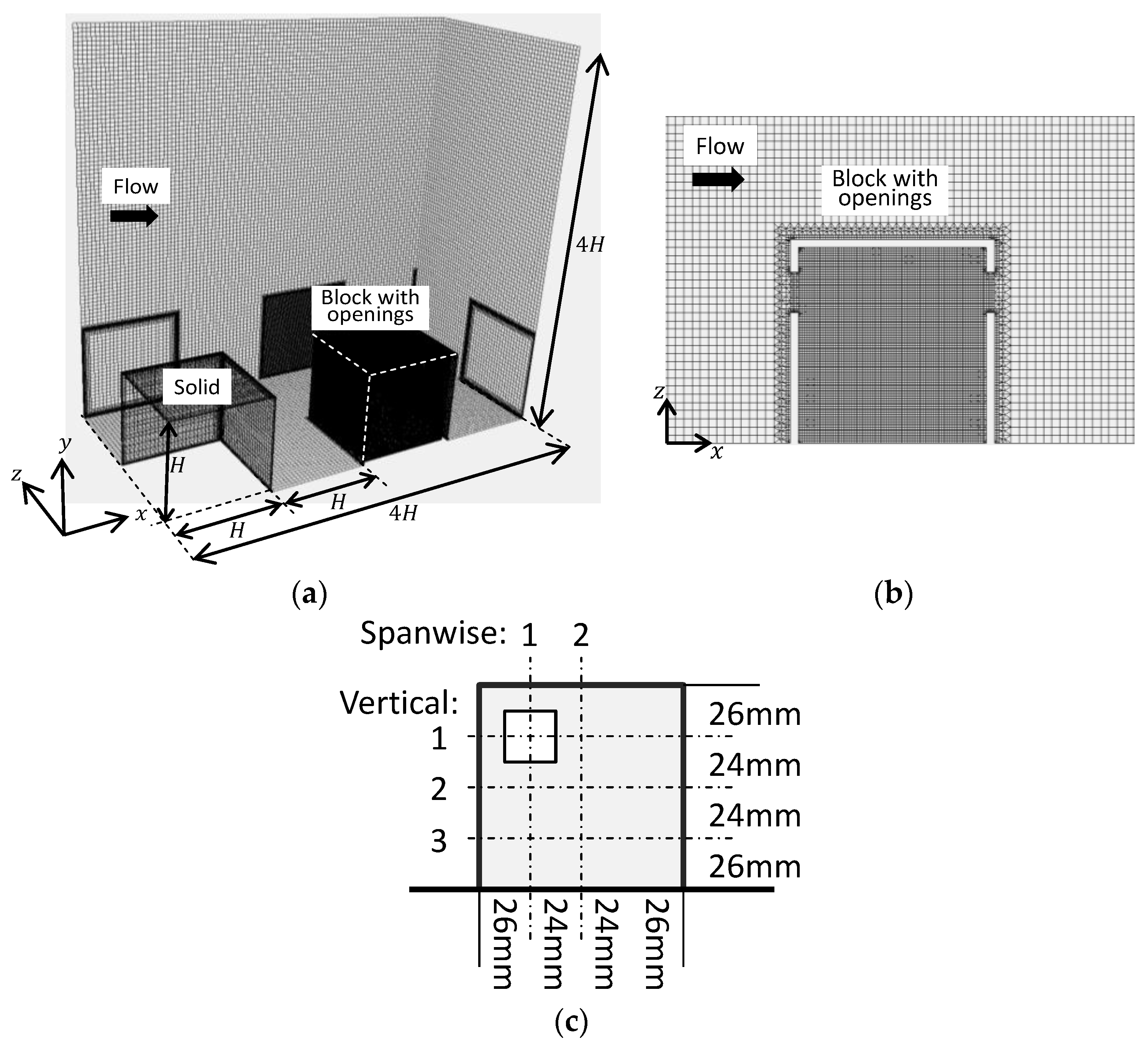
Figure 1a provides an overview of the calculation domain. Cyclic boundary conditions are imposed at spanwise and streamwise boundaries to reproduce an infinitely-repeated array of cubical blocks with 25% block coverage, or a so-called lattice-square type building array. It is known that exterior flow regimes near the rectangular block change by the block coverage ratio from the isolated flow regime for sparse conditions to the skimming flow regime for dense conditions [20]. Skimming flow with steady vortices inside the block cavity is expected to be formed in the present condition. Since indoor ventilation of the building in the building array might be significantly different from a building in open spaces because of a characteristic steady vortex in the canyon due to surrounding buildings in dense conditions, we adopted the present building array conditions, and focus on the effect of opening positions. Various surrounding building conditions will be discussed in future work. The block height $H$ is 100 mm. Flow is driven by a constant streamwise pressure gradient $dp/dx$, determined by experimental data [21] to achieve an average wind speed in the yz-plane of $u_{bulk}=8$ m/s, in which flow over the building array is independent of the Reynolds number. This constant flow condition is similar to the flow field generated in wind-tunnel experiments, but differs from those observed in outdoor flow fields, in which both the wind speed and direction temporally change. However, as a first step to clarify the effect of opening locations on indoor ventilation with surrounding conditions, the present simulations were performed under the identical wind speed conditions. A zero gradient boundary condition is imposed at the top of the domain for velocity and scalar quantities. No-slip boundary condition is imposed at the block and floor surfaces.

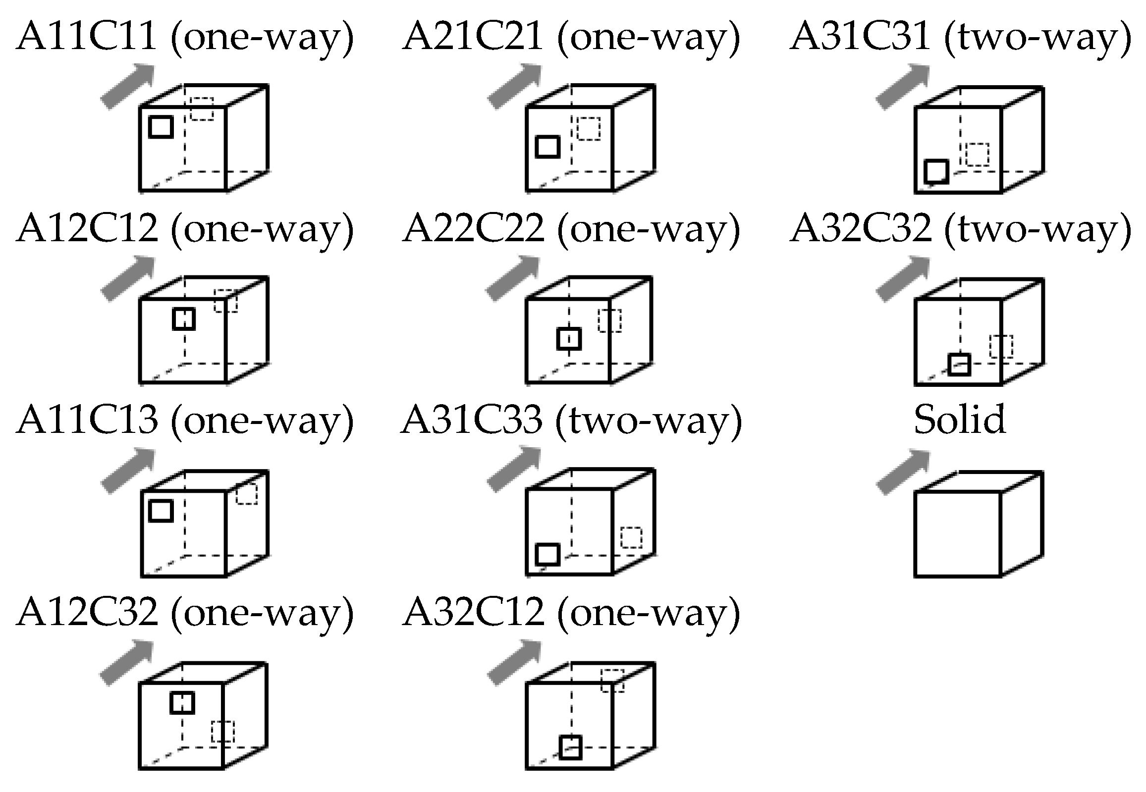
Figure 1a indicates a numerical mesh with a solid building and the building with square openings of $A=400$ mm² ($l_{op}=20$ mm). Details of the mesh near openings are shown in Figure 1b. The inside of the block is void space with a wall thickness of 4 mm. Uniform grids of $H/25$ were employed for the x-, y-, and z-directions, except for building openings and interiors, which had grid sizes of $H/100$. Walls with openings were divided into four meshes in the streamwise direction. These grid resolutions can satisfy the recommendations of the previous studies. Namely, at least 1/10 grids of building height are recommended for the RANS simulation of the outdoor flow field, as a guideline [22]. In addition, Ito et al. [23] have shown that only two grids at the inlet position does not cause a large discrepancy in the indoor flow field distributions. The definitions of the openings are shown in Figure 1c, and the positions of the openings were chosen from three locations, denoted as 1, 2, and 3, in the vertical, and 1 and 2 in the spanwise directions. In order to investigate the effects of opening locations, including the relative locations of both openings, 10 combinations of opening positions on the windward and leeward walls were selected as shown in Figure 2, where windward and leeward are denoted by A and C, respectively. In addition, the solid case was also investigated as a reference condition.

Steady-state flow and pressure fields are solved by employing RANS and continuity equations with the SIMPLE (semi-implicit method for pressure-linked equations) algorithm by using OpenFOAM 2.2.1 (OpenCFD Ltd. (ESI Group), Barknell, UK). The Launder Sharma k-ε model (low Reynolds number k-ε model [24]) is used for the turbulence model by solving budget equations of TKE $k$ and energy dissipation rate $\epsilon$. In order to perform the sensitivity study of the turbulence model for flow fields of both indoor and outdoor spaces, reliable flow field data are necessary. Unfortunately, such flow field data, which cover both indoor and outdoor regions, are not available presently; therefore, only one type of low Reynolds number model is selected by considering co-existence of laminar, transient to turbulent, and turbulent flow in the present simulation condition. In terms of the exterior flow fields, mean wind profiles and turbulence statistics were compared with previous results of numerical simulations, as explained in Section 3.1.

A second-order linear interpolation scheme is employed for advection and diffusion terms of velocity, turbulent kinetic energy $k$, and dissipation rate $\epsilon$. In order to avoid the numerical oscillation for velocity fields due to advection terms, the first-order upwind schemes are blended up to 20% only at the position where numerical oscillation can be detected. Details of the scheme, which is implemented OpenFOAM 2.2.1, is explained in Okeze et al. [25]. Convergence of the flow fields were decided by monitoring the flow field distributions on the horizontal plan and vertical profile of the horizontally-averaged streamwise wind speed.

The building-height Reynolds number of this simulation scale is approximately $5.3\times {10}^4$, so that the dependence of the building’s exterior space on the Reynolds number becomes negligible [26]. Contrarily, the Reynolds number defined by the opening length scale $l_{op}=20$ mm and the wind speed normal to the openings (approximately 0.25 m/s to 5.25 m/s, depending on the opening position) ranges from $3.3\times {10}^2$ to $7\times {10}^3$. Under the condition of ${\left(l_{op}/H\right)}^2~0.05$, the volume flow rate becomes an almost constant value when the opening Reynolds number is greater than ${10}^4$ according to the empirical equation of the discharge coefficient of a thin-plate orifice [27]. In the present simulations, however, even the largest opening Reynolds number is less than the criterion. Although we have to state that flow distributions through openings might be turbulent or laminar, the relationships between the ventilation rates and flow introduction patterns are successfully explained in Section 3.2 and Section 3.3. Therefore, the present simulation can give valuable knowledge regarding the mechanism of indoor ventilation, though the Reynolds number dependency of the flow distribution within the openings of the building in the block array must be examined in further study.

3. Results

3.1. Flow and Pressure Fields

Figure 3 shows vertical profiles of the horizontally averaged streamwise velocity $u$, TKE $k$, and vertical Reynolds stress $-\overline{u^{\prime }{w}^{\prime }}$ for six selected cases of Solid, A12C12, A22C22, A32C32, A12C32, and A32C12. Reference profile data of velocity and Reynolds stress are obtained from Coceal et al. [28]. The vertical Reynolds stress is calculated based on gradient transport theory with the eddy viscosity. The values inside the block are excluded from spatial averaging to compare flows of outdoor spaces. The wind speed is normalized by the reference wind speed defined at $2H$. TKE and Reynolds stress are scaled by the friction velocity defined as $u^{\ast }=\sqrt{L_z/\rho \left(dp/dx\right)}$, where $L_z$ indicates the domain height, and $\rho$ represents the air density. Profiles from Coceal et al. [28] in the figures are determined by direct numerical simulation. As can be seen in the figure, these six case profiles of mean wind speed, TKE, and Reynolds stress are quite similar to one another, both within and above the canyon region. This result indicates that the effect of air flow from the outlet of the wall openings to the outdoor area is minimal in the spatially-averaged sense because of the large differences between the mean wind speed and TKE in the canyon region compared to the outlet flow from the wall openings. Though other cases are not shown in the figure, almost identical profiles are obtained for all statistics.

In general, the streamwise wind speed profiles over $1H$ show good agreement with those of Coceal et al. [28]. On the other hand, the profiles inside the canyon show discrepancies: the profiles here increase almost linearly with height within the canopy layer, whereas those of Coceal et al. [28] show a slight convex curve below $0.5H$ and a concave curve above $0.5H$. Furthermore, the Reynolds stress profiles of the present study shows an upward convex curve below $1H$; however, that value determined by Coceal et al. [28] shows a large gradient near the bottom and top of the canopy. Though there is no reference data for TKE in the canopy layer for the square array to compare, it might be expected that the underestimations of TKE can happen in the canopy layer, as explained in Xie and Castro [29], resulting in an almost linear slope of the velocity inside the canyon due to insufficient eddy diffusivity. Although the Launder Sharma k-ε model cannot reproduce velocity profiles inside the canopy for streamwise wind speed with high accuracy in this calculation situation, comparable velocity fields both above and within the canopy layer were reproduced by RANS simulation.

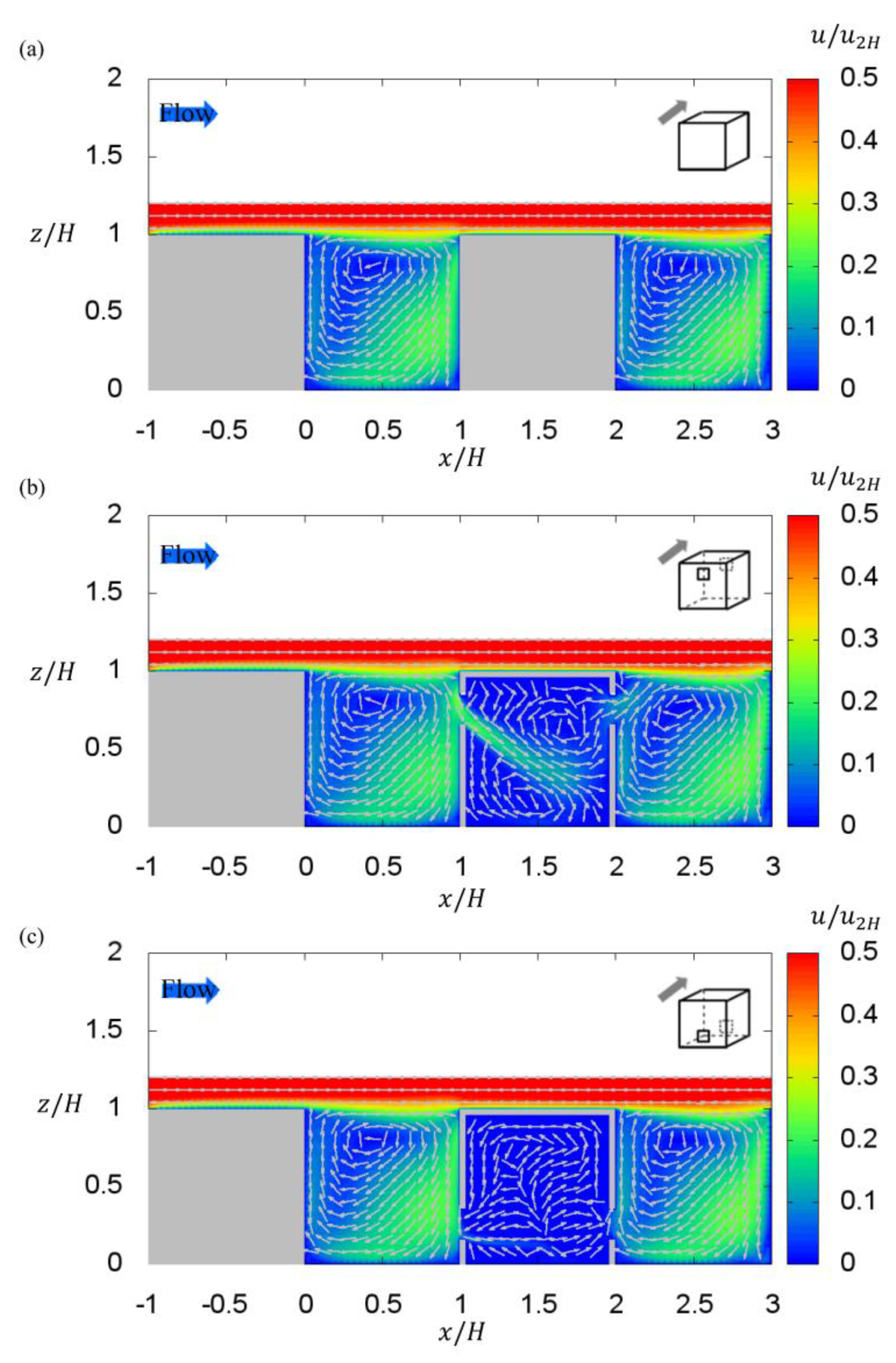
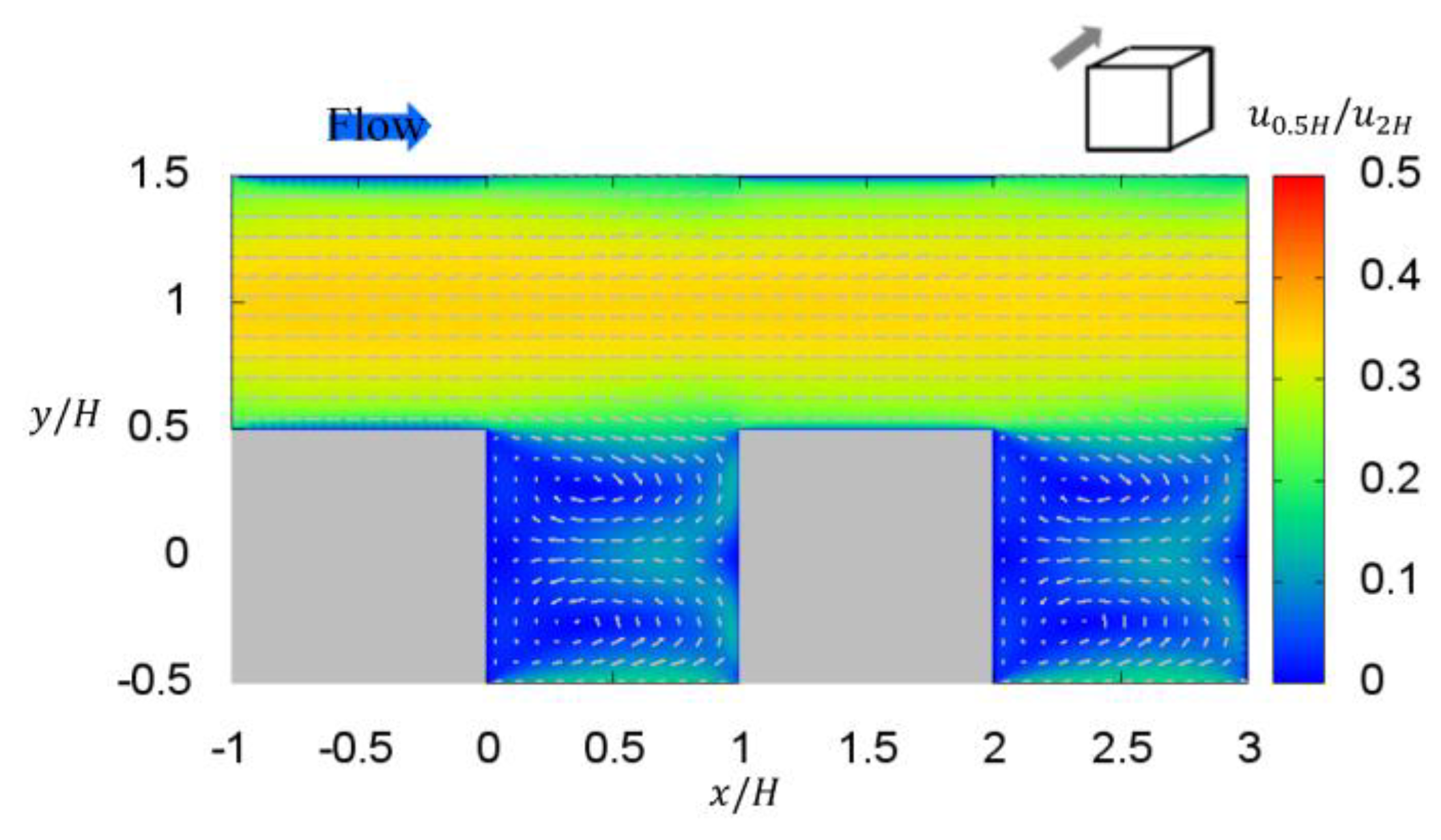
Exterior flow fields are shown in Figure 4 and Figure 5. Figure 4 shows sectional views of the flow fields at the spanwise centres of the buildings for three cases that are typical of the flow patterns among all 11 cases: solid, A12C12, and A32C32. In the figure, only the contours and vectors below $1.2H$ are shown for clarity. The solid case in Figure 4a shows that recirculation flows exist between buildings. These flow patterns are well known as skimming flow [20]. The formation of the skimming flow can also be conformed in Figure 5, which shows the horizontal sectional flow fields of the solid case at $z=0.5H$. The high velocity flows in the open spaces between $y=0.5H$ to $1.5H$ are introduced into the canyon region between two buildings. These flows cause high-speed regions along the right and left faces of the windward wall, resulting in the counter-rotating cortex pair reported by Coceal et al. [28]. The sectional flow field presented in Figure 4b for A12C12, where the openings are located in the upper row, shows a jet flow from the windward opening into the room. The jet is neither vertical nor perpendicular to the windward wall, but flows diagonally into the room because of the recirculation flow in the outside canyon region. Moreover, a flow is also observed from the leeward opening to the canyon region behind the building. The leeward jet merges with the recirculation flow outside the room. Although the jet flows can be observed at both windward and leeward openings, the jet flows nonetheless have minimal effects on the outside recirculation flow. The sectional flow field presented in Figure 4c for A32C32, where the openings are located in the lower row, shows that, in this case, ventilation flow appears to be very weak. A weak jet perpendicular to the opening can be seen at the bottom edge of the windward opening. As in A12C12, the presence of the openings has very little effect on the outdoor flow fields. Section 3.2 presents a more detailed discussion of the flows in the openings.

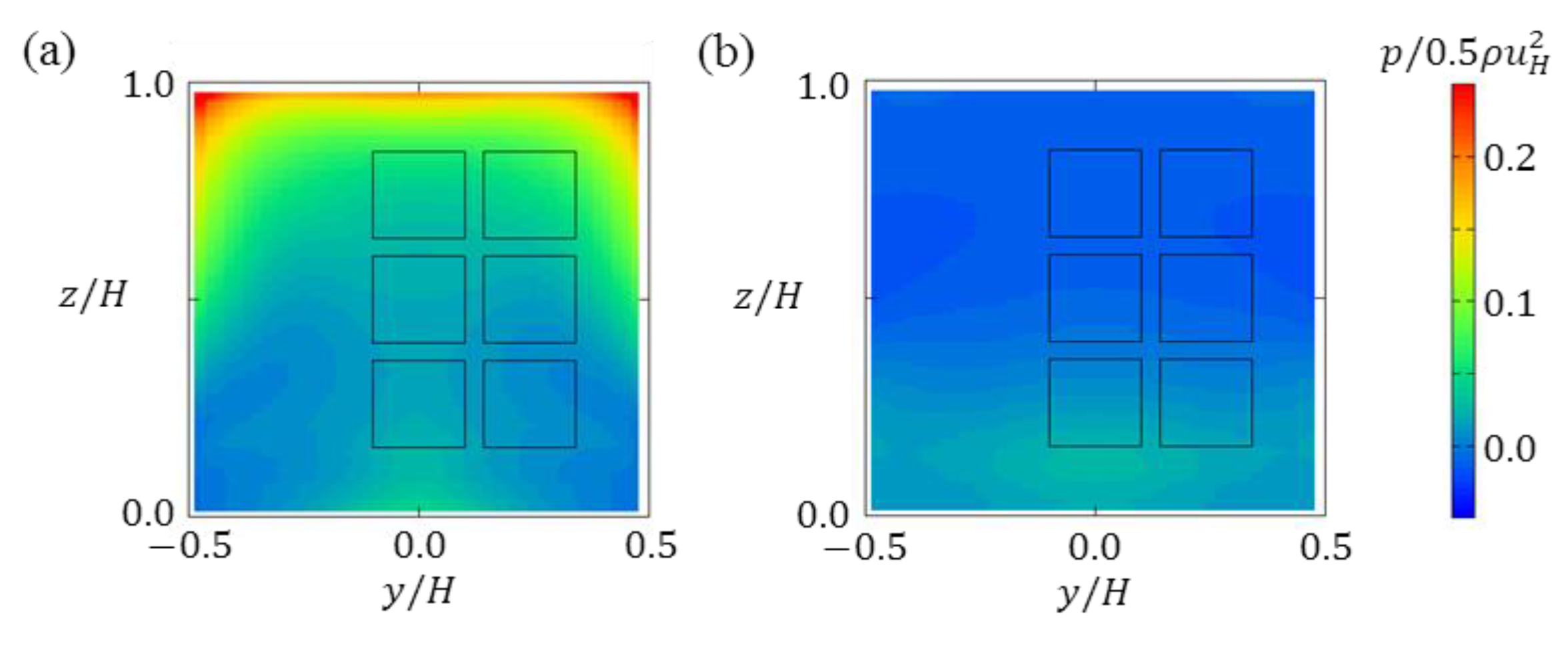
The wall pressures due to the flow fields near the buildings are important to estimate the ventilation efficiencies of the buildings; therefore, Figure 6a,b show the pressure coefficient distributions of the Solid case’s windward and leeward walls, respectively. The rectangles on the figures represent the opening locations of the other cases. On the windward wall, the pressure values generally become larger at higher locations. On the upper half of the buildings, larger pressure values can be observed along the edges, whereas on the lower half, pressure is higher near the spanwise centre. This is because fast winds blow against the building’s upper parts, resulting in a large dynamic pressure contribution to the wall pressure. Conversely, in the building’s lower parts, wind flows toward the spanwise centre along with the windward wall due to counter vortices, which are attributed to the small wall pressure because of the large dynamic pressure of the flow itself. Figure 6b shows the pressure distribution on the leeward wall. In contrast to the windward wall, the relative values of the pressure coefficients on this face are considerably smaller, and some negative values can be observed. In particular, the pressure values at higher positions are significantly smaller because of recirculation flow in the canyon, which generates flows away from the leeward wall.

Although these wall pressure distributions on cube faces in a block array are qualitatively similar to those obtained by LES [10] and wind-tunnel experiments [29], we have to state that RANS simulation may not capture even relative distributions of the pressure distribution. According to Xie and Castro [30], the vertical gradient of laterally-integrated pressure coefficients near the block roof level of cubes become steeper by the standard $k$-$\epsilon$ model than those obtained by LES. Zaki et al. [29] reported pressure coefficients of cubes in block arrays for three arrangement patterns with five packing densities. By interpolating their data to 25% packing density in order to compare our simulation results, the pressure coefficient $C_p=\langle \Delta p\rangle /0.5\rho U_H^2$, where $\langle \Delta p\rangle =\langle p_f\rangle -\langle p_b\rangle$ indicates the block-face averaged pressure differences between front and back faces, which is estimated as 0.12. Contrary, the coefficient becomes 0.05 in the present simulation for solid block, meaning that pressure values of the present simulation are underestimated by more than 60%.

According to these flow and pressure distributions, the RANS simulation reproduces qualitative outdoor flow and pressure fields for the purpose of generating skimming flow interacting with surrounding building arrays, although quantitative difference can been significant especially for turbulence statistics and block wall pressure.

These discrepancies indicate that further quantification of the ventilation rates based on wall pressure values and turbulence statistics might cause considerable differences as compared with those determined by LES or DNS. However, the detailed analyses of various combinations of opening positions can advance a qualitative understanding of the relationship between flow fields and ventilation efficiency. In addition, error estimation of TKE can show how the mean flow and turbulence can affect the ventilation rates. Therefore, results of the RANS-type simulation should be examined well in the next section.

3.2. Flows in Building Openings

As can be seen in the recirculation flow patterns presented in Section 3.1, the presence of openings has very little effect on the flow fields of outdoor spaces. However, flows introduced through openings may differ considerably depending on the opening positions, with some positions promoting more effective indoor ventilation. Therefore, this section discusses flow distribution patterns in the openings of windward and leeward walls in order to categorize flow introduction types through openings.

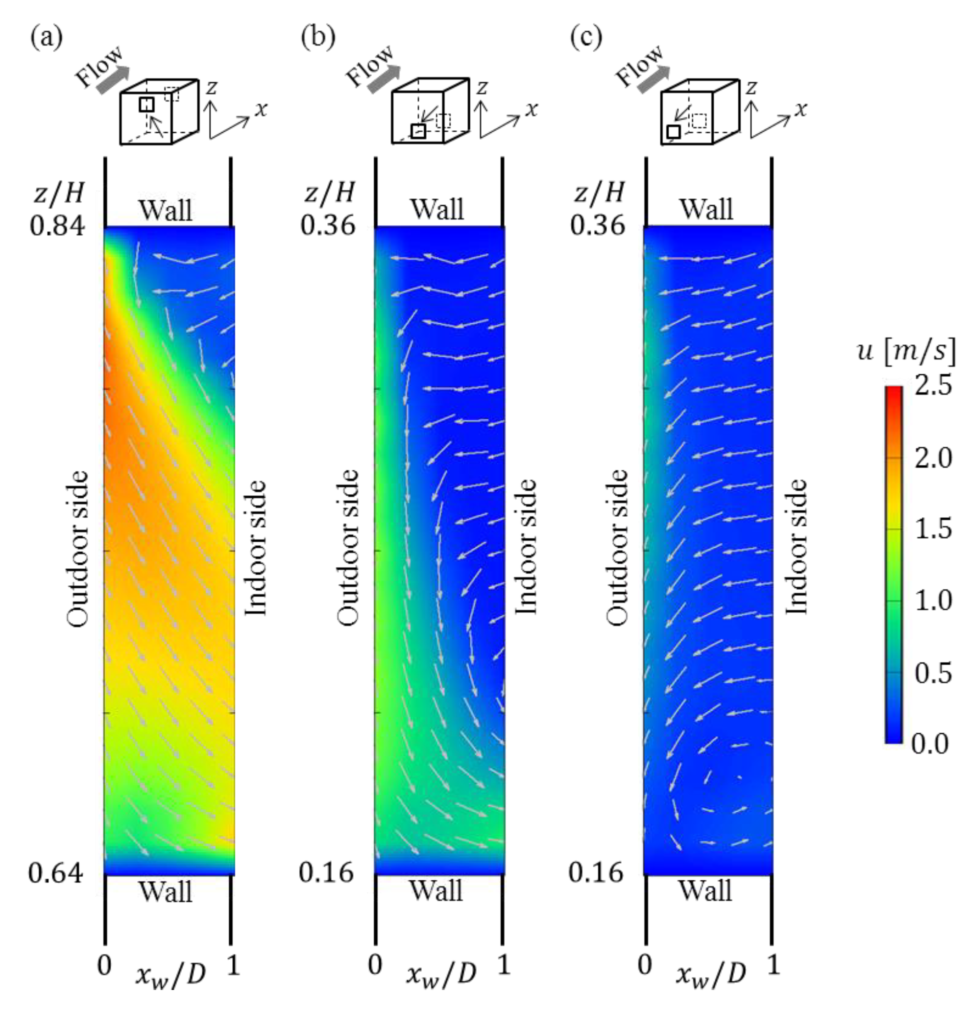
Figure 7 shows vertical sectional flow fields in windward openings at the spanwise centres of the three typical cases. Figure 7 only illustrates flow distributions within openings. The horizontal axis $x_w/D$ represents the coordinates from the windward wall normalized by wall thickness D. Though both of xz and xy cross-sectional views were confirmed, the xz cross-sections are suitable for the following flow categorization. In A12C12, where the openings are in the upper row, wind blows diagonally downward through the openings in most of the regions with large wind speeds, which is why the flows are introduced into the room diagonally, as shown in Figure 4b. In addition, a triangular reverse flow region can be observed near the upper corner of the interior side. In contrast, in A32C32, where the openings are in the lower row, the wind direction is almost downward as it approaches the exterior side after passing through the opening, and then the flow returns to the bottom edge of the opening. As a result, only air flows from the lower parts are introduced into the room with a wind direction that is normal to the opening. In most of the openings, a reverse flow can be observed though the opening of the windward wall. Similar reverse flows are seen in the case of A31C31, where openings are also located in the lower row, as shown in Figure 7c. In this case, a vortex appears at $z=18$ mm; air flows are introduced into the room below the vortex, whereas flows are ejected from the room above the vortex.

In the same manner, vertical sectional flow fields in the windward openings of all cases were visualized and classified into the following two types: the one-way type is characterized by air flows that are unidirectional, such as the downward diagonal of A12C12, and the two-way type is characterized by air flows that are introduced into the room at the bottom edges of the openings and ejected out from the room in the upper regions of openings, such as A32C32 and A31C31. Following this classification, the three cases of A32C32, A31C31, and A31C33 were two-way, and the other seven cases were one-way (schematic figures are summarized in Figure 9).

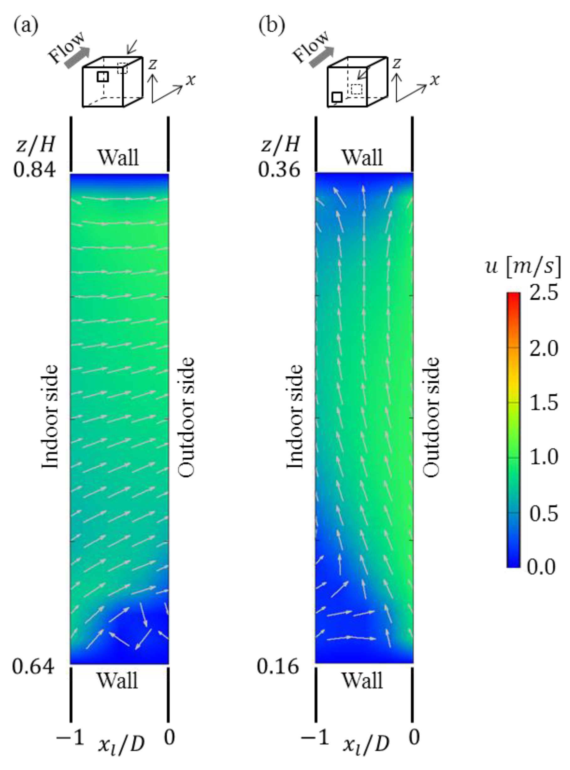
Flow patterns in the leeward openings were also categorized as either the one-way or two-way type. Figure 8 shows the vertical sectional flow fields in the leeward openings for two typical cases. Horizontal axis $x_l/D$ represents the coordinates from the leeward wall normalized by the wall thickness D. In A12C12, flows with almost homogeneous wind speeds blow perpendicular to the opening. In contrast, the wind direction of A31C31 is almost parallel to the openings and upward. The upward flow in the opening volume is generated by flow introduced at the bottom edge of the opening from both sides of the room and from the leeward canyon. Accordingly, air flows are ejected into both the room and leeward canyon from the opening volume at the top edge. Eventually, all cases classified as either the one-way type or two-way type at the windward opening were also classified as the same type at the leeward opening.

3.3. Various Ventilation Rate Definitions

In order to quantify the ventilation efficiency differences due to opening locations, four ventilation rates are calculated in this section: net ventilation rate $Q_{net}$, gross ventilation rate $Q_{gross}$, estimated cumulative and average instantaneous ventilation rate $Q_{ins}$, and the conventional ventilation rate $Q_{conv}$. These ventilation rates are defined in detail as follows:

The conventional ventilation rate $Q_{conv}$ was calculated from wall pressure differences $\Delta p$ of the Solid case as expressed in the following equations:

$$Q_{conv}=A_{eff}\sqrt{\frac{2\Delta p}{\rho }}$$

(1)

$${\left(\frac{1}{A_{eff}}\right)}^2={\left(\frac{1}{\alpha A_{front}}\right)}^2+{\left(\frac{1}{\alpha A_{rear}}\right)}^2$$

(2)

Here, $\rho$ is the air density; $\alpha$ is the flow rate coefficient (or discharge coefficient) (=0.6) (White, 2010); $A_{front}=A_{rear}$ (=0.02² m²) as the front and rear opening areas, respectively; and $A_{eff}$ is the effective opening area. Since the conventional method calculates the introduction flow speed by pressure differences between openings between based on the Bernoulli’s theorem, flow in indoor and outdoor spaces are assumed to diffuse perfectly, indicating openings should be small enough. In addition, correct flow rates need to be determined based on flow introduction angles. According to previous research, conventional methods estimate ventilation rates reasonably when wall porosity is less than 10% [2]. Advantages of the conventional methods are easiness of determining the ventilation rates as first approximation only based on wall pressure distribution, though correct flow rates are needed. In the present estimation, pressure difference $\Delta p$ is determined by the pressure distribution of solid conditions.

As shown in Section 3.2, there are reverse flows in the openings in the several cases classified as two-way ventilation and, therefore, these reverse flows must be considered to accurately quantify the ventilation efficiency. The net ventilation rate $Q_{net}$ regards the reverse flow as negative ventilation. In other words, $Q_{net}$ is determined by the streamwise mean wind speed ${\overline{u}}_{op}$ times the opening area $A$ as expressed as follows:

$$Q_{net}={\Sigma }_i{\overline{u}}_i\Delta A_i={\overline{u}}_{op}A$$

(3)

Here, ${\overline{u}}_i$ and $\Delta A_i$ represent the streamwise mean wind speed and opening area at simulation node $i$ located in the opening. The conventional method in Equation (1) is thought to estimate this ventilation rate by approximating the flow introduction speed based on pressure differences. The net ventilation rates are thought to be more accurate than the conventional method; however, the wind speed averages in openings are needed for determination. The wind speed averages in openings were determined by simulated results for calculating the net ventilation rates for each case.

On the other hand, the gross ventilation rate $Q_{gross}$ regards the reverse flow as positive ventilation:

$$Q_{gross}={\Sigma }_i\left|{\overline{u}}_i\right|\Delta A_i.$$

(4)

Therefore, the gross ventilation rate can be defined individually for the windward and leeward sides. This treatment of reverse flow is the simplest and most often used method in coupled simulations of indoor and outdoor areas [9]. Contrarily, spatial distributions of wind speeds in openings are necessary for determining the gross ventilation rate. Therefore, it might be difficult to determine the rate except for flow fields obtained by CFD. In the present estimation, spatial distributions of wind speeds were determined by CFD to derive the gross ventilation rates.

Although the present simulation is based on steady-state analysis, the effect of turbulent flow exchange on ventilation efficiency is another factor that must be considered. Therefore, the cumulative and average instantaneous ventilation rate $Q_{ins}$ was estimated by assuming a normal distribution of fluctuating wind speeds through openings following Caciolo et al. [7]. Instantaneous wind speeds $u_i^{\prime }\left(t\right)$ are approximated by 10⁶ random numbers following a normal distribution with a standard deviation by eddy diffusivity and the mean velocity gradient (following eddy viscosity theory with eddy viscosity ${\nu }_t=c_{\mu }k/\epsilon$, where $c_{\mu }=0.09$). The cumulative and average instantaneous ventilation rate $Q_{ins}$ is determined by integrating the absolute values of estimated instantaneous wind speeds as follows:

$$Q_{ins}=\frac{1}{T}\int {\Sigma }_i\left|{\overline{u}}_i+u_i^{\text{'}}\left(t\right)\right|\Delta A_{i}dt$$

(5)

Under the realistic condition of the urban boundary layer, exterior flow fields are turbulent in most cases; therefore, the instantaneous ventilation rate is the most realistic volume flow rate which can express air exchange between indoor and outdoor spaces. On the other hand, the ventilation rates require temporal and spatial distribution of wind speeds in openings, indicating assumptions are needed to determine the turbulent contribution on the ventilation as we followed from Cionco et al. [7] when a RANS-type simulation was employed. According to the previous LES of flow and pressure field data for the same block arrangements conducted by Ikegaya et al. [10], the probability density of the wall pressure coefficient on both windward and leeward walls can be regarded as a normal distribution because even the maximum skewness was only 0.17 near the opening position of A11. Therefore, the assumption of a normal distribution of fluctuating wind speed through openings is considered plausible for estimating the turbulent contribution to ventilation. We have to state that, however, the accuracy of standard deviation by present RANS simulation might be insufficient for quantifying instantaneous effect, as can be seen in the Reynolds stress profile in Figure 3c. According to Xie and Castro [30], the RANS simulation underestimates the TKE values in the canopy layer as compared with LES for an urban-like array, and the underestimation ratios of RANS to LES can be estimated as approximately 30% based on the vertical profiles of TKE [30]. Therefore, the cumulative and averaged instantaneous ventilation rates with TKE values increased by 30% from the RANS simulation results are also calculated in order to quantify the expected ranges of instantaneous ventilation.

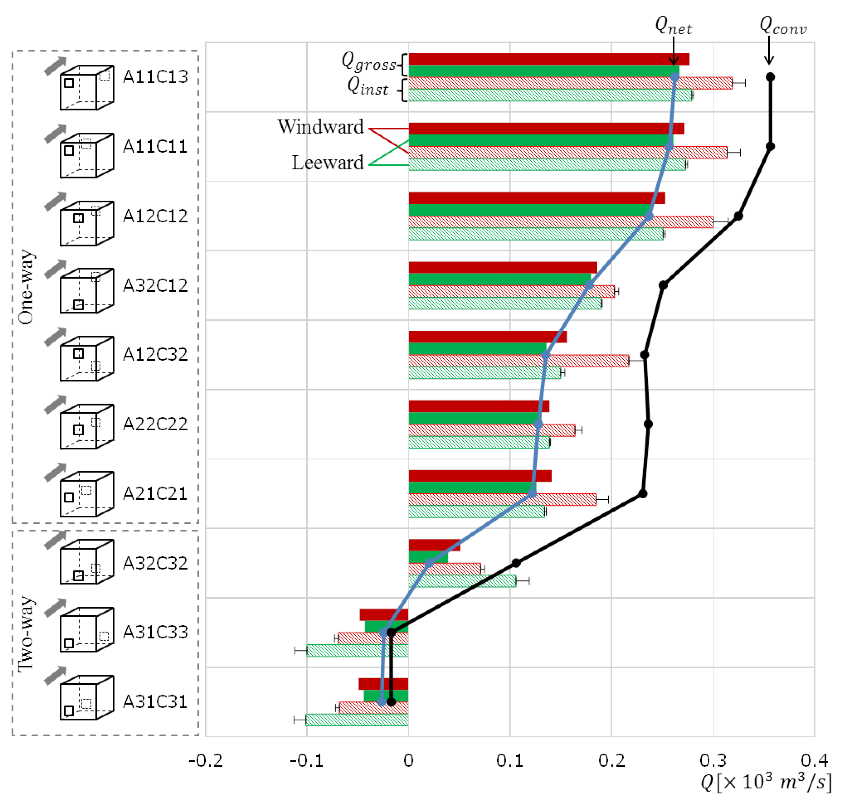
The ventilation rates of all 10 cases are compared in Figure 9. $Q_{gross}$ and $Q_{ins}$ were individually determined at each windward and leeward opening because these values are unequal, depending on the flow distribution in the openings. The error bar on $Q_{ins}$ indicates expected values when TKE increased 30%. In general, both windward and leeward openings in the higher row (A11C13, A11C11, and A12C12) produced high ventilation rates. In contrast, cases where the openings were in the bottom row on both windward and leeward walls (A32C32, A31C33, and A31C31) produced low ventilation rates. These results are considerably natural because inlets or outlets in upper positions can be exposed to flow with larger wind speed. Moreover, surprisingly, A31C33 and A31C31 showed reversed ventilation, indicating that the net flow direction was from the leeward opening to the windward opening ($Q_{gross}$ and $Q_{ins}$ are always positive, but are shown to be negative in comparison with their $Q_{net}$ and $Q_{conv}$ magnitudes). These values are simply due to stronger positive or negative wind wall pressure near the higher opening position on the building’s windward or leeward wall.

In cases of one-way ventilation, $Q_{ins}$ is larger than $Q_{gross}$, although $Q_{net}$ and $Q_{gross}$ are almost comparable. Therefore, turbulent ventilation can enhance indoor ventilation even when one-way flow through openings is dominant, though increasing rates due to turbulence are not so significant as compared with the total ventilation rates. Even though the expected increase of TKE is considered, the qualitative tendency that $Q_{ins}$ is slightly larger than $Q_{gross}$ does not change because the mean flow mainly determined the ventilation rates, and the contribution of turbulent ventilation is significant for one-way ventilation. In contrast to the one-way types, the ratios of $Q_{net}$ to $Q_{gross}$ are large in two-way types because inflow and outflow can occur simultaneously through the same openings. Moreover, the difference in the ratios of $Q_{net}$ and $Q_{ins}$ for the two-way ventilation is especially large at the leeward opening. This may be due to upward shear flows, which can promote turbulence ventilation. The turbulence effect may have grate impact on two-way ventilations as can be seen the expected increasing rate of $Q_{ins}$ due to 30% appreciation of TKE. Lastly, in the cases of one-way ventilation, $Q_{conv}$ and $Q_{net}$ showed similar trends for each of the opening locations, whereas the $Q_{net}$ values were always 40% smaller than the $Q_{conv}$ values. As shown in Section 3.2, wind flows that are directed diagonally downward through an opening into the room result in decreased flow rate coefficients (Vickery and Karakatsanis [31]). Therefore, $Q_{net}$ yields a smaller value than $Q_{conv}$. This result indicates that conventional methods are applicable when flows introduced through openings are one-way ventilation even for the building in the building array; however, estimating the effective opening area, including the flow rate coefficient, is important for the flow affected by the surrounding building arrays based on the wind direction through the openings. Conversely, such as the two-way ventilation cases, estimating the ventilation flow rates by the conventional method can be difficult because of reverse or turbulent flow near, and within, the openings.

4. Conclusions

Coupled simulations of air flows in and among outdoor and indoor spaces in a building array were performed by taking a RANS approach. A simplified building arrangement was modelled with a block coverage ratio of 25%. One of the buildings had openings on the windward and leeward walls, and the inside space was also solved explicitly. A total of 10 combinations of opening positions were selected to investigate the effect of opening positions on ventilation rates. The conclusions are summarized as follows:

First, characteristics of outdoor flow fields were confirmed for both the solid case and opening cases. As can be seen in the flow visualization of the vertical cross section, a recirculating vortex exists between two buildings in both the opening and solid cases. Although a strong introduction of flow into the room through openings and jet flow from the room to the outdoor canyon region can be confirmed, flows related to the opening had very little effect on the outdoor recirculation flow pattern, resulting in similar skimming flows in all 11 cases, even with the openings. Moreover, the velocity, Reynolds stress, and TKE profiles above the building array for all 11 cases were quite similar to each other. Therefore, the interaction between the urban boundary layer flow and indoor ventilation is considered to be unidirectional for ventilation due to the steady-state flow, and perhaps the recirculation region within the block canyon can be separated from the urban boundary layer in a more sophisticated investigation of ventilation efficiency in a building array. In addition to the flow fields, wall pressure distributions of windward and leeward walls for the solid case shows similar tendency to those obtained by WTE and LES.

Secondly, the flow introduction patterns though openings are classified based on detailed observation of the flow distributions, focusing on the opening volumes in both the windward and leeward walls. The flow patterns can be categorized into two types: in the one-way type, flows are introduced diagonally through openings in one direction, and in the two-way type, flows are both introduced to, and ejected from, the room through the same opening. These classifications are shown to elucidate the mechanisms that cause indoor ventilation, although the flow introduction patterns are classified only qualitatively based on the visualized flow images.

Lastly, to quantify the effects of the opening locations, ventilation rates were determined by the following four definitions: conventional, net, gross, and cumulative and average instantaneous. In general, openings in the higher row produced higher ventilation rates, whereas openings in the lower row produced lower ventilation rates. Although these findings are not surprising, these differences in the ventilation rates were shown to be strongly related to the flow introduction classifications. In one-way ventilation, air flows are introduced into the room diagonally downward at the windward opening and ejected perpendicularly from the opening in the leeward wall. Since one-way flow in openings is dominant, the net and gross air change rates were comparable in the one-way ventilation cases. Moreover, the cumulative and instantaneous ventilation rate, which considers the estimated fluctuating velocity, was always larger than the net air change rate. Furthermore, the conventional method was found to overestimate the ventilation rate by approximately 40% because of the inclination angle of flow through openings causing a reduction of the flow rate coefficient. In contrast to one-way types, the gross ventilation rates of two-way types were considerably larger than their net ventilation rates because of reverse flow through the same openings. In addition, the cumulative ventilation rates at the opening in the leeward wall were the largest because of the upward shear flow near the opening.

The RANS simulations employed in this study could be improved in terms of accuracy of the estimation of cumulative and average instantaneous ventilation rates. However, various configurations are necessary to quantify the relationships between indoor ventilation efficiency and building shapes, opening locations, surrounding block arrangements, and so on. As can be seen, clear relationships between flow introduction types and ventilation rates, present CFD successfully identify the impact of opening locations even though RANS simulations were employed. In addition, differences between conventional and net flow rates imply that flow rate coefficient (or discharge coefficient) might be reduced due to the flow introduction angle through the openings. Therefore, we believe that RANS simulations are advantageous to investigate various building conditions, based on the results presented here, which provide sufficiently quantifying relationships between the opening flow regime and ventilation efficiency. In addition, it is a plausible strategy that overall tendencies are examined by RANS simulations as a first step. Contrarily, more accurate simulation would be necessary for quantifying the effects of complex flow fields due to both spatial distribution and turbulent effect on ventilation flow rates.

References

- Ramponi, R.; Blocken, B. CFD simulation of cross-ventilation for a generic isolated building: Impact of computational parameters. Build. Environ. 2012, 53, 34–48. [Google Scholar] [CrossRef] [Green Version]
- Seifert, J.; Li, Y.; Axley, J.; Ro, M. Calculation of wind-driven cross ventilation in buildings with large openings. J. Wind. Eng. Ind. Aerodyn. 2006, 94, 925–947. [Google Scholar] [CrossRef]
- Asfour, O.S.; Gadi, M.B. A comparison between CFD and Network models for predicting wind-driven ventilation in buildings. Build. Environ. 2007, 42, 4079–4085. [Google Scholar] [CrossRef]
- Jiang, Y.; Alexander, D.; Jenkins, H.; Arthur, R.; Chen, Q. Natural ventilation in buildings: Measurement in a wind tunnel and numerical simulation with large-eddy simulation. J. Wind Eng. Ind. Aerodyn. 2003, 91, 331–353. [Google Scholar] [CrossRef]
- Ai, Z.T.; Mak, C.M. Analysis of fluctuating characteristics of wind-induced air flow through a single opening using LES modeling and the tracer gas technique. Build. Environ. 2014, 80. [Google Scholar] [CrossRef]
- Wang, H.; Chen, Q. A new empirical model for predicting single-sided, wind-driven natural ventilation in buildings. Energy Build. 2012, 54, 386–394. [Google Scholar] [CrossRef]
- Caciolo, M.; Stabat, P.; Marchio, D. Full scale experimental study of single-sided ventilation: Analysis of stack and wind effects. Energy Build. 2011, 43, 1765–1773. [Google Scholar] [CrossRef]
- Lo, L.J.; Banks, D.; Novoselac, A. Combined wind tunnel and CFD analysis for airflow prediction of wind-driven cross ventilation. Build. Environ. 2013, 60, 12–23. [Google Scholar]
- Jiang, Y.; Chen, Q. Study of natural ventilation in buildings by large eddy simulation. J. Wind Eng. Ind. Aerodyn. 2001, 89, 1155–1178. [Google Scholar] [CrossRef] [Green Version]
- Ikegaya, N.; Hirose, C.; Hagishima, A.; Tanimoto, J. Effect of turbulent flow on wall pressure coefficients of block arrays within urban boundary layer. Build Environ. 2016, 100, 28–39. [Google Scholar] [CrossRef]
- Gough, H.; Sato, T.; Halios, C.; Grimmond, C.S.B.; Luo, Z.; Barlow, J.F.; Robertson, A.; Hoxey, R.; Quinn, A. Effects of variability of local winds on cross ventilation for a simplified building within a full-scale asymmetric array: Overview of the Silsoe field campaign. J. Wind Eng. Ind. Aerodyn. 2018, 175, 408–418. [Google Scholar] [CrossRef]
- King, M.F.; Gough, H.L.; Halios, C.; Barlow, J.F.; Robertson, A.; Hoxey, R.; Noakes, C.J. Investigating the influence of neighbouring structures on natural ventilation potential of a full-scale cubical building using time-dependent CFD. J. Wind Eng. Ind. Aerodyn. 2017, 169, 265–279. [Google Scholar] [CrossRef]
- Kurppa, M.; Hellsten, A.; Auvinen, M.; Raasch, S.; Vesala, T.; Järvi, L. Ventilation and air quality in city blocks using large-eddy simulation-urban planning perspective. Atmosphere 2018, 9, 65. [Google Scholar] [CrossRef]
- Liu, F.; Qian, H.; Zheng, X.; Zhang, L.; Liang, W. Numerical study on the Urban ventilation in regulating microclimate and pollutant dispersion in Urban street Canyon: A case study of Nanjing new region, China. Atmosphere 2017, 8, 164. [Google Scholar] [CrossRef]
- Abd Razak, A.; Hagishima, A.; Ikegaya, N.; Tanimoto, J. Analysis of airflow over building arrays for assessment of urban wind environment. Build Environ. 2013, 59, 56–65. [Google Scholar] [CrossRef]
- Kubota, T.; Miura, M.; Tominaga, Y.; Mochida, A. Wind tunnel tests on the relationship between building density and pedestrian-level wind velocity: Development of guidelines for realizing acceptable wind environment in residential neighborhoods. Build Environ. 2008, 43, 1699–1708. [Google Scholar] [CrossRef]
- Yoshie, R.; Tanaka, H.; Shirasawa, T.; Kobayashi, T. Experimental study on air ventilation in a built-up area with closely-packed high-rise buildings. J. Environ. Eng. AIJ 2008, 73, 661–667. (In Japanese) [Google Scholar] [CrossRef]
- Bo, M.; Salizzoni, P.; Clerico, M.; Buccolieri, R. Assessment of indoor-outdoor particulate matter air pollution: A review. Atmosphere 2017, 8, 136. [Google Scholar] [CrossRef]
- Kapwata, T.; Language, B.; Piketh, S.; Wright, C.Y. Variation of Indoor Particulate Matter Concentrations and Association with Indoor/Outdoor Temperature: A Case Study in Rural Limpopo, South Africa. Atmosphere 2018, 9, 124. [Google Scholar] [CrossRef]
- Oke, T.R. Street Design and Urban Canopy Layer Climate. Energy Build. 1988, 11, 103–113. [Google Scholar] [CrossRef]
- Hagishima, A.; Tanimoto, J.; Nagayama, K.; Meno, S. Aerodynamic parameters of regular arrays of rectangular blocks with various geometries. Bound.-Layer Meteorol. 2009, 132, 315–337. [Google Scholar] [CrossRef]
- Tominaga, Y.; Mochida, A.; Yoshie, R.; Kataoka, H.; Nozu, T.; Yoshikawa, M.; Shirasawa, T. AIJ guidelines for practical applications of CFD to pedestrian wind environment around buildings. J. Wind Eng. Ind. Aerodyn. 2008, 96, 1749–1761. [Google Scholar] [CrossRef]
- Ito, K.; Inthavong, K.; Kurabuchi, T.; Ueda, T.; Endo, T.; Omori, T.; Ono, H.; Kato, S.; Sakai, K.; Suwa, Y.; et al. CFD Benchmark Tests for Indoor Environmental Problems: Part 1 Isothermal/Non-Isothermal Flow in 2D and 3D Room Model. Int. J. Arch. Eng. Technol. 2015, 2, 1–22. [Google Scholar] [CrossRef]
- Launder, B.E.; Sharma, B.I. Application of the energy-dissipation model of turbulence to the calculation of flow near a spinning disk. Lett. Heat Mass Transf. 1974, 1, 121–138. [Google Scholar] [CrossRef]
- Okaze, T.; Kikumoto, H.; Ono, H.; Imano, M.; Hasama, T.; Kishida, T.; Nakao, K.; Ikegaya, N.; Tabata, Y.; Tominaga, Y. Large-eddy simulations of flow around a high-rise building-validation and sensitivity analysis on turbulent statistics. In Proceedings of the 7th European and African Conference on Wind Engineering, Liege, Belgium, 3–6 July 2017. [Google Scholar]
- Uehara, K.; Wakamatsu, S.; Ooka, R. Studies on critical Reynolds numbef indices for wind tunnel experiments on flow qithin urban areas. Bound.-Layer Meteorol. 2003, 107, 353–370. [Google Scholar] [CrossRef]
- White, F.M. Fluid Mechanics, 7th ed.; McGraw-Hill: New York, NY, USA, 2010. [Google Scholar]
- Coceal, O.; Thomas, T.G.; Belcher, S.E. Spatial variability of flow statistics within regular building arrays. Bound.-Layer Meteorol. 2007, 537–552. [Google Scholar] [CrossRef]
- Zaki, A.S.; Hagishima, A.; Tanimoto, J. Journal of Wind Engineering Experimental study of wind-induced ventilation in urban building of cube arrays with various layouts. J. Wind Eng. Ind. Aerodyn. 2012, 103, 31–40. [Google Scholar] [CrossRef]
- Xie, Z.; Castro, I.P. LES and RANS for turbulent flow over arrays of wall-mounted obstacles. Flow Turbul. Combust. 2006, 76, 291–312. [Google Scholar] [CrossRef]
- Vickery, B.J. External wind pressure distributions and induced internal ventilation flow in low-rise industrial and domestic structure. ASHRE Trans. 1987, 93 Pt 2, 2198–2213. [Google Scholar]
Figure 1.
Schematic of the numerical simulation target: (a) simulation domain with numerical grids; (b) side view of the mesh arrangement for the block with openings (case A12C12); and (c) the definition of the opening positions.
Figure 2.
Combinations of windward and leeward openings: A and C indicate the windward and leeward walls, respectively, and the subsequent numbers indicate the vertical and spanwise positions of the openings, respectively.
Figure 3.
Vertical profiles of (a) streamwise wind speed; (b) turbulence kinetic energy; and (c) vertical Reynolds stress for Solid, A12C12, A22C22, A32C32, A12C32, and A32C12 with reference from Coceal et al. [28]. Present simulation data, except for the Solid case, are plotted every four vertical grid points for clear presentation.
Figure 4.
Sectional views of flow fields at the spanwise centre of the block: below for (a) Solid; (b) A12C12; and (c) A32C32.
Figure 5.
Plan view of flow field at for the Solid case.
Figure 6.
Wall pressure distribution on solid block on the (a) windward wall and (b) leeward wall. Black rectangles indicate positions of openings.
Figure 7.
Sectional view of flow fields at spanwise centre of windward opening for (a) A12C12; (b) A32C32; and (c) A31C31. is coordinate of at windward wall. represents the wall thickness.
Figure 8.
Sectional view of flow fields at spanwise centre of leeward openings for (a) A12C12 and (b) A31C31. is coordinate of at leeward wall. represents the wall thickness.
Figure 9.
Ventilation rates for each opening position. : determined by conventional method by Equation (1), : net ventilation rate by Equation (3), : gross ventilation rate by Equation (4), and : estimated cumulative and average instantaneous ventilation rate. The error bar in indicates the rate with a 30% increase of TKE by reflecting the underestimation of TKE in the present simulation as compared with those of LES (Xie and Castro [30]).
© 2018 by the authors. Licensee MDPI, Basel, Switzerland. This article is an open access article distributed under the terms and conditions of the Creative Commons Attribution (CC BY) license (http://creativecommons.org/licenses/by/4.0/).
Share and Cite
MDPI and ACS Style
Murakami, Y.; Ikegaya, N.; Hagishima, A.; Tanimoto, J. Coupled Simulations of Indoor-Outdoor Flow Fields for Cross-Ventilation of a Building in a Simplified Urban Array. Atmosphere 2018, 9, 217. https://doi.org/10.3390/atmos9060217
AMA Style
Murakami Y, Ikegaya N, Hagishima A, Tanimoto J. Coupled Simulations of Indoor-Outdoor Flow Fields for Cross-Ventilation of a Building in a Simplified Urban Array. Atmosphere. 2018; 9(6):217. https://doi.org/10.3390/atmos9060217
Chicago/Turabian StyleMurakami, Yuki, Naoki Ikegaya, Aya Hagishima, and Jun Tanimoto. 2018. "Coupled Simulations of Indoor-Outdoor Flow Fields for Cross-Ventilation of a Building in a Simplified Urban Array" Atmosphere 9, no. 6: 217. https://doi.org/10.3390/atmos9060217
Note that from the first issue of 2016, this journal uses article numbers instead of page numbers. See further details here.