Dynamic and Thermodynamic Factors Associated with Different Precipitation Regimes over South China during Pre-Monsoon Season

Abstract

Nine precipitation regimes over South China are obtained by applying the Self-Organizing Map (SOM) technique to the sub-daily precipitation during the pre-monsoon season (April to June) of 1979–2015. These nine regimes are distinct from each other in terms of precipitation amount and spatial pattern. The relationships between precipitation and different atmospheric dynamic and thermodynamic factors (large-scale divergence, water vapor flux, low-level jet, precipitable water, convective available potential energy (CAPE), and K index) are explored under the nine regimes. The upper-level divergence performs best in indicating the geographic positions of precipitation centers, which are also modulated by the orientations of low-level jets. The estimation of water vapor transport reveals that there are two major moisture sources for the precipitation during the pre-monsoon season, i.e., the Bay of Bengal (for all the nine regimes) and the South China Sea and West Pacific Ocean (for five regimes). Furthermore, the occurrence probability of more precipitation increases with the water vapor transported from the South China Sea and West Pacific Ocean. Compared to CAPE, K index performs better in indicating the precipitation centers and has a tighter relationship with area-average precipitation. The precipitable water exhibits complicated relationships with spatial patterns and amounts of precipitation, indicating that it may be not a good indicator for precipitation during pre-monsoon season over South China. Estimation of the persistence and transformation probabilities for precipitation regimes reveals that the persistence probabilities basically decrease with the precipitation amounts, and the transformations between different precipitation regimes are inclined to be associated with the southward shifts of precipitation centers.

1. Introduction

South China, a region with the most abundant precipitation over East Asia, has a long rainy season lasting from April to September. During the rainy season, the precipitation amount shows a dual-peak mode [1]. The precipitation amount reaches the first peak during the pre-monsoon season (April to June). The April to June (AMJ) precipitation accounts for more than 40% of the annual precipitation over most parts of South China [2], and is even more than that in Spring (accounting for about 35%) [3,4] or Summer (about 35%) [4] over South China. The precipitation during AMJ has profound impacts on human society and natural environment over South China [5]. For example, in April 2011, the precipitation in Fujian Province was less than usual, which led to the lack of sufficient potable water for more than 300,000 people and drought in more than 500 km² of farmland. By contrast, the heavy precipitation during the AMJ over South China in 2016 resulted in severe disasters including landslides, debris flows, and urban/rural waterlogging, and the direct economic losses related to the heavy precipitation totalled more than one billion dollars. Therefore, exploring the mechanisms behind the AMJ precipitation over South China, which provides a theoretical basis for the skilful predictions, is essential.

However, compared to the summer monsoon precipitation, or wintertime precipitation [6,7,8,9,10,11,12,13,14,15,16,17,18], fewer studies focused on the precipitation during AMJ over South China. Zhao et al. [19] examined the mesoscale characteristics of a heavy rainfall event over Hong Kong during pre-monsoon season. Specifically, a front with an upward motion branch ahead of the front, a southerly branch trough, a southerly warm and moist current contributed to water vapor transport and strong horizontal wind convergence, a series of meso $\beta$ systems, and shallow disturbances in the low-level atmosphere were found to be associated with the heavy rainfall event. Gu et al. [2] investigated the interannual variations of precipitation during pre-monsoon season and the related mechanism. Basically, the precipitation during pre-monsoon season lasts about 90 days spanning from 6 April to 4 July. Their study revealed that an east–west SST dipole anomaly in the tropical Pacific would excite an anomalous anticyclone near Philippines in the lower troposphere, which favored the subsequent moisture convergence, strong ascending motions and thus more precipitation over South China. Based on composite analysis for the whole rainy season (AMJ), Ding and Wang [1] analyzed the climatological characteristics of the low-level circulation (wind fields on 850 hPa) and water vapor transport, and quantitatively estimated the moisture budgets for the precipitation over South China. They pointed out that the strengthened rainfall during AMJ over South China was associated with weakening of cold air activities, intensified southwest monsoonal circulation, and water vapor transports. By comparing the composite AMJ moisture fluxes under the years with normal, anomalously more, and anomalously less precipitation over South China, Chen et al. [20] revealed that the water vapor transport from the South China Sea had a crucial influence on the precipitation amount during AMJ over South China. Note that Ding and Wang [1] treated the precipitation over South China during AMJ as a whole, but the precipitation during AMJ may be associated with different amounts and spatial patterns. Similarly, Chen et al. [20] treated the AMJ precipitation as a whole. Although they classified the AMJ precipitation into three groups, the classification was only based on precipitation amounts. As pointed by Trenberth et al. [21], the characteristics of precipitation, i.e., intensity, frequency, and spatial pattern, are as important as the amount. Besides, the precipitation is always related to multiple atmospheric dynamic and thermodynamic factors, and may be related to or modulated by many other systems, such as atmospheric blocking, El Niño/Southern Oscillation, Pacific Decadal Oscillation [3,6,11,22,23,24]. However, most previous studies on AMJ precipitation over South China only analyzed individual dynamic and thermodynamic factors, which is incomplete for analyzing the relationship between AMJ precipitation and atmospheric dynamic and thermodynamic factors. Therefore, this study will examine the characteristics of precipitation with different amounts and spatial patterns during AMJ over South China, and explores the relationships between precipitation and multiple atmospheric dynamic and thermodynamic factors.

Most of the extreme precipitation events have a time scale of less than one day. Therefore, exploring the characteristics of the AMJ precipitation from the sub-daily perspective is necessary. To deal with the enormous sub-daily precipitation data, a classification of precipitation into different precipitation regimes is an effective way. In this study, a neural network-based classification technique, i.e., Self-Organizing Map (SOM) technique proposed by Kohonen [25], is used to classify the AMJ sub-daily precipitation over South China into different precipitation regimes. Up to date, SOM was widely used in the climate community [26,27,28,29,30,31,32,33]. In addition, the previous studies have pointed out that the persistence and transformation characteristics among different regimes benefit the weather forecast [34,35,36]. To systematically explore the relationships between precipitation regimes and the associated meteorological factors, three dynamic factors including large-scale divergence, water vapor flux and low-level jet and three thermodynamic factors including precipitable water, CAPE and K index are analyzed in our study. Heavy precipitation, especially the persistent heavy precipitation, is one of the factors that causes severe meteorological disasters [37,38]. South China is one of the regions where the persistent extreme precipitation events prefer to occur [39]. In our study, the heavy precipitation events and persistent heavy precipitation events during AMJ over South China are analyzed from the perspective of regimes.

Our study focuses on the relationship between different precipitation regimes and associated meteorological factors, the persistence and transformations of the precipitation regimes, and analyzing the heavy precipitation events during AMJ over South China from the perspective of precipitation regimes. The study is organized as follows. We introduce the data, clustering method and meteorological factors in Section 2. Section 3.1 is devoted to validating of the precipitation data used in our study, determining the optimal number of regimes, and describing the precipitation regimes. Section 3.2 and Section 3.3 discuss the dynamic and thermodynamic factors associated with different precipitation regimes, respectively. The persistence and transformations of the precipitation regimes are analyzed in Section 3.4 and the heavy precipitation events are investigated in Section 3.5. In Section 4, we summarize our study.

2. Data and Methods

2.1. Data

The data used in this study are mainly taken from the European Center for Medium-Range Weather Forecasts (ECMWF) ReAnalysis Interim (ERA-Interim) [40] for the period of 1979–2015. The horizontal resolution of the ERA-Interim reanalysis system is approximately 79 km (T255; a reduced Gaussian grid with 512 × 256 points). The variables under analysis include air temperature, horizontal winds, specific humidity, relative humidity, and divergence on pressure levels. Other variables include precipitation, convective available potential energy (CAPE), and surface pressure. Compared with the reanalysis system, the variables under analysis have different horizontal resolutions. Specifically, all the variables are available on a uniform 1.5° longitude–latitude grid with 240 × 121 points except that the precipitation is on a uniform 0.75° longitude–latitude grid with 480 × 241 points. The time resolution of all the variables from the ERA-Interim is 12-hourly. Totally, there are 6734 time levels under consideration during AMJ 1979–2015 (3367 days, each day with two time levels). In addition, the monthly precipitation data from Global Precipitation Climatology Centre (GPCC) [41] during AMJ 1979–2015 are used to validate the ERA-Interim precipitation data, and the precipitation data during 1979–2014 from surface stations compiled by the China Meteorological Administration are used to verify the precipitation regimes.

2.2. Self-Organizing Map

The SOM technique is used for identifying precipitation regimes over South China during AMJ. SOM is an unsupervised neural network-based classification technique, which can represent the multidimensional datasets by a limited number of neurons/regimes distributed on a topological map [42,43,44]. On the topological map, the neighboring regimes usually share some common similarities, while the separated regimes are associated with distinct characteristics [45]. Assume that there are N input samples/vectors (in this study, N equals 6734), i.e., $x_1$, $x_2$, …, $x_N$, and these N samples are projected to a SOM map with X regimes. Note that the number of regimes X is defined by user and each regime is a vector $w_j$ (j = 1, 2, 3, …, X) with the same dimension as the input sample. The SOM algorithm can be summarized as follows. First, the initial regimes are initialized by the principal component analysis (PCA) method [46]. Second, the Euclidean distance between the input sample $x_i$ (i = 1, 2, 3, …, N) and each regime is calculated. The regime that has the minimum Euclidean distance is recognized as the best-matching unit $w_b$ (BMU). Third, the regimes in the neighborhood of BMU are updated according to the following equation:

$$w_j(t+1)=w_j(t)+\alpha (t)h_{bj}(t)[x_i-w_j(t)],$$

(1)

where t is the time step, $\alpha (t)$ is the learning rate, and $h_{bj}(t)$ is the neighborhood function. Both the learning rate and neighborhood function decrease with time. Fourth, the second and third steps are repeated until all the N input samples are covered. Finally, the above three steps are iterated until the iterative condition is reached.

2.3. Dynamic and Thermodynamic Factors

In this study, we used six meteorological factors to analyze the characteristics associated with different precipitation regimes over South China during AMJ 1979–2015: large-scale divergence (convergence), water vapor flux for the lower troposphere, low-level jet, precipitable water, CAPE, and K index. These six factors can be classified into two groups. The first group includes the dynamic factors large-scale divergence (convergence), water vapor flux in the lower troposphere, and low-level jet. The second group includes the thermodynamic factors precipitable water, CAPE, and K index.

Large-scale divergence (convergence) in the lower troposphere provides the dynamic circulation background, which may inhibit (promote) the occurrence of precipitation. Specifically, the circulation pattern associated with low-level convergence and upper-level divergence favors the convergence of water vapor in the atmospheric boundary layer and further leads to the uplift of air masses, which increases the probability of precipitation.

One of the most important components of Asian monsoon system is water vapor transport [47], which is also one of the necessary conditions for the precipitation. Here, we use the water vapor flux to represent the transport of water vapor. Compared to the convergence of water vapor flux, the flux form of the water vapor transport is more easily linked to the dynamic circulation pattern (e.g., the low-level jet) and more beneficial to the moisture source analysis for the precipitation. According to Feng and Zhou [48], the water vapor flux is calculated as

$$\left\{\begin{array}{c}{Q}_x=\frac{1}{p_t-p_s}(\frac{1}{g}{\int }_{p_s}^{p_t}qudp)\hfill \\ Q_y=\frac{1}{p_t-p_s}(\frac{1}{g}{\int }_{p_s}^{p_t}qvdp)\hfill \end{array},\right.$$

(2)

where $Q_x$ and $Q_y$ are the zonal and meridional water vapor fluxes; $p_t$ and $p_s$ are the pressures at 600 and 1000 hPa, respectively; g is the acceleration of gravity; q is the specific humidity; $(u,v)$ are the zonal and meridional winds; and p is the pressure coordinate.

Low-level jet, which is characterized by a fast-moving airstream in the lower troposphere [49], is conducive to the occurrence of heavy precipitation events since it could provide abundant water vapor [50,51]. In addition to the water vapor transport, the positive vorticity produced by the cyclonic shear of the wind speed on the left side of the jet stream has the ability to enhance the convergence in the low levels, which is also favorable to the precipitation [52]. The low-level jet is usually defined as the wind belts with magnitudes larger than a threshold in the lower troposphere [53,54]. In this study, we used the winds on 850 hPa to define the low-level jet, and adopted 8 m s⁻¹ as the threshold.

The precipitation is closely related to the precipitable water, i.e., the increase in precipitable water is in favor of more precipitation [55,56]. For each grid cell, precipitable water is defined as the amount of precipitation if all the water vapor (in the corresponding column) condense and precipitate to the ground. The calculating formula for precipitable water ($PW$) is as follows, i.e.,

$$PW=\frac{1}{g}{\int }_{P_s}^{P_t}qdp,$$

(3)

where $P_s$ is the surface pressure and $P_t$ is the pressure at the top of atmosphere.

Convective precipitation is a major precipitation type and is always associated with obvious weather phenomena such as lighting and thunder. Different types of convection even lead to different levels of threat to life and property. As revealed by Kastman et al. [57], compared to surface based convection, elevated convection favors more severe lightning and heavier rainfall. CAPE is used to evaluate the convective potential for the atmosphere, i.e., the energy with which the air parcel could keep rising when there are no external forces [58,59,60]. CAPE plays a dominant role in the genesis and maintenance of convective precipitation [61]. Specifically, CAPE is estimated as the vertically integrated energy generated by the buoyancy and has the following formula:

$$\mathrm{CAPE}={\int }_{z_0}^{z_t}g\frac{T_{v,p}-T_{v,e}}{T_{v,e}}dz,$$

(4)

where $z_0$ is the height of free convection; $z_t$ is the height of equilibrium level; $T_{v,p}$ and $T_{v,e}$ are the virtual temperatures of air parcel and environment, respectively; and z is the vertical coordinate.

K index is an aggregative indicator for atmospheric stability and the degree of saturation of water vapor [62]. The calculating formula for the K index is

$$K=(T_{850hPa}-T_{500hPa})+T_{d,850hPa}-(T_{700hPa}-T_{d,700hPa}),$$

(5)

where T is temperature and $T_d$ is the dew point temperature.

3. Results

3.1. Identification of Precipitation Regimes

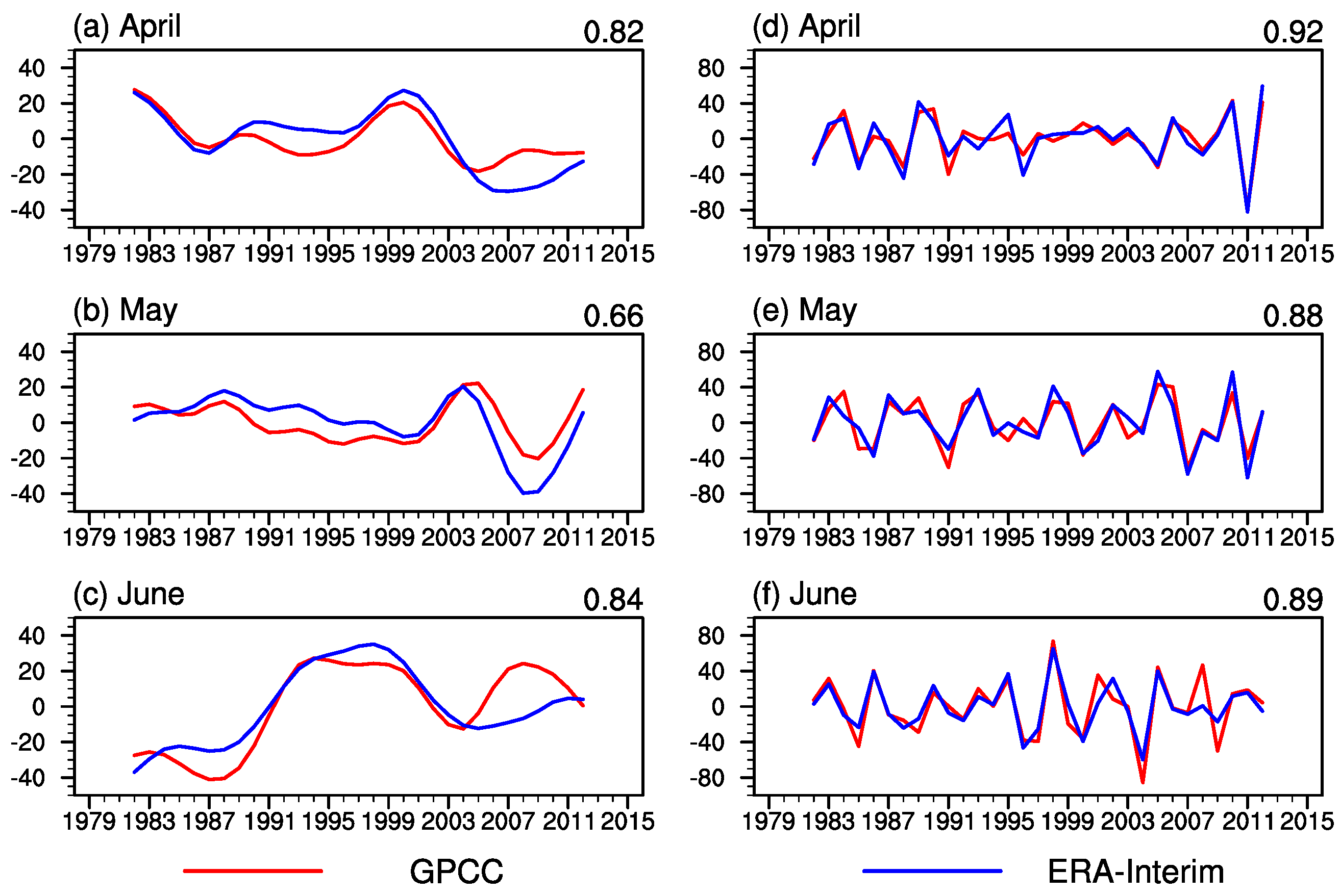
3.1.1. Validation of the ERA-Interim Precipitation Data

Before applying the SOM technique to identify the precipitation regimes, the reliability of the ERA-Interim precipitation data is validated first. The observed precipitation data, i.e., GPCC, are used to validate the ERA-Interim precipitation data. Because the time frequency of GPCC is monthly, the 12-hourly precipitation data of ERA-Interim are used to estimate the monthly precipitation for ERA-Interim (to make a comparison). As shown in Figure 1a–c, the major parts of the observed rain bands during AMJ are located over the coastal areas of South China, which are well reproduced by the ERA-Interim dataset (Figure 1d–f). The ERA-Interim dataset also captures the positions of observed maxima in precipitation during the months under consideration. In addition, the observed increase of precipitation over South China with time (from April to June) is successfully reproduced by the ERA-Interim dataset.

The performance of the ERA-Interim precipitation data is further validated by studying its relationship with the observed data on the interdecadal and interannual time scales, respectively. The mean values of the area-averaged precipitation over South China (105–123° E, 21.5–32° N) during AMJ 1979–2015 are 206.82 mm month⁻¹ and 196.46 mm month⁻¹ for ERA-Interim and GPCC, respectively, indicating that the AMJ precipitation of ERA-Interim is a bit overestimated over the South China region. Figure 2 shows the time evolutions of the area-averaged precipitation anomalies over South China for April, May, and June, respectively. The interdecadal (>10 year) and interannual (<10 year) components of the area-averaged precipitation anomalies were obtained by applying the seven-point Lanczos filter [63]. The correlations between the area-averaged precipitation anomalies of ERA-Interim and that of observation for the three months all exceed 0.66 at the interdecadal time scale, which are comparatively large. The correlations at the interannual time scale for the three months range from 0.88 to 0.92, which are even higher than those at the interdecadal time scale. Therefore, both the horizontal distributions and the time evolutions of the precipitation from ERA-Interim are reasonable over South China during AMJ 1979–2015.

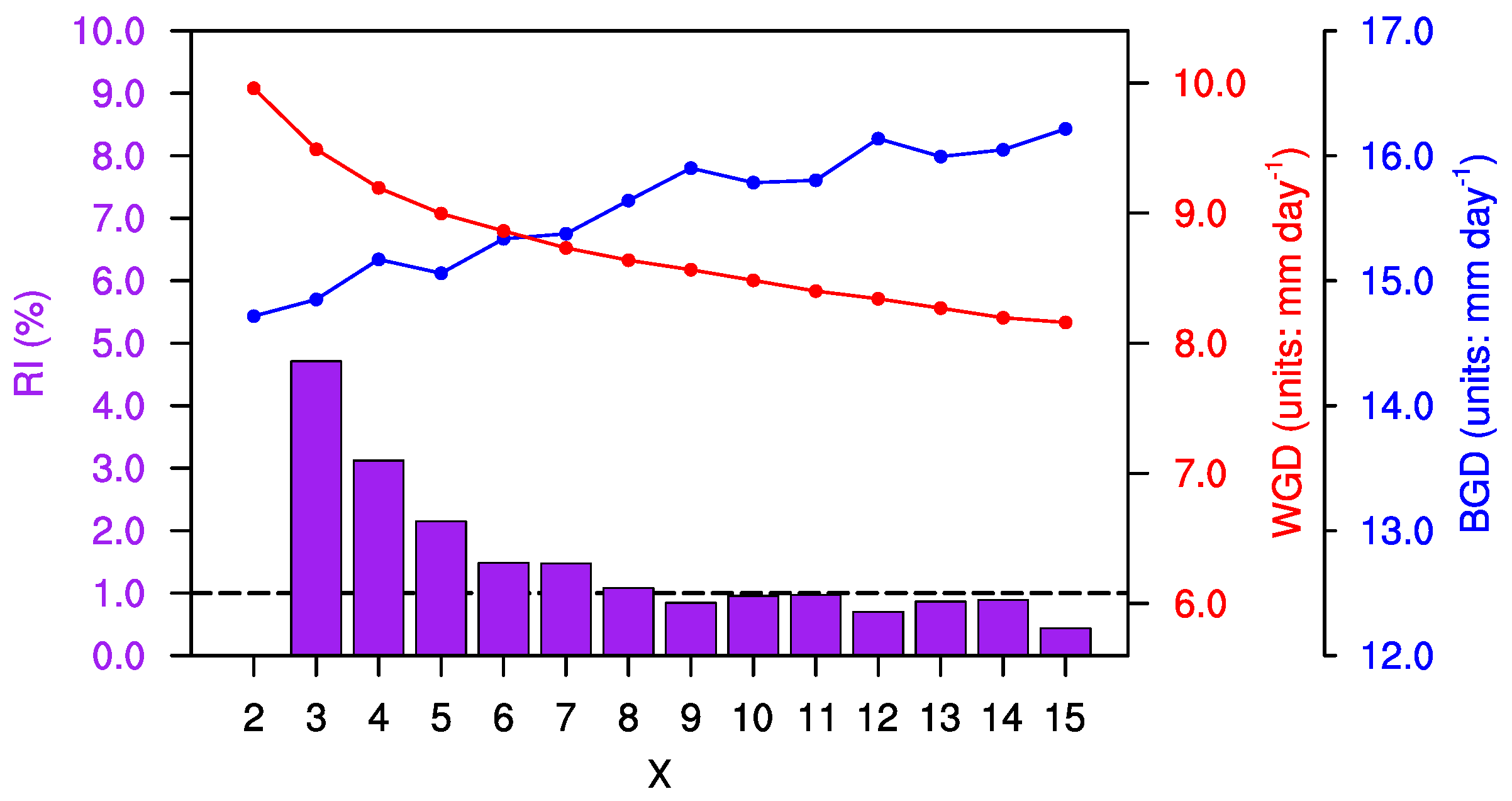
3.1.2. The Optimal Number of Regimes

As mentioned in Section 2.2, the number of regimes X is defined by the user. To find the optimal value for X, we define two metrics, i.e., within-group distance (WGD) [36,64,65] and between-group distance (BGD) [36,66,67]. WGD is calculated as

$$\mathrm{WGD}=\frac{1}{N}\sum _{k=1}^N{\left(\frac{{\sum }_{i=1}^n{\sum }_{j=1}^m{W}_{i,j}{(O_{i,j,k}-R_{i,j,k})}^2}{n\times m}\right)}^{\frac{1}{2}},$$

(6)

where N is the total number of samples (6734 samples in this study) and k is the index for each sample; n and m are the numbers of grid cells along the zonal and meridional directions; i and j are the indices for grid cells along the zonal and meridional directions; $W_{i,j}$ is the area weight for the corresponding grid cell $(i,j)$; $O_{i,j,k}$ is the original precipitation value of grid cell $(i,j)$ for sample k; and $R_{i,j,k}$ is the precipitation value of grid cell $(i,j)$ for the precipitation regime that sample k belongs to. BGD is calculated as

$$\mathrm{BGD}=\frac{1}{N}\sum _{k=1}^N\left[\frac{1}{X-1}\sum _{k^{\prime }=1}^{X-1}{\left(\frac{{\sum }_{i=1}^n{\sum }_{j=1}^m{W}_{i,j}{(O_{i,j,k}-R_{i,j,k^{\prime }}^{\prime })}^2}{n\times m}\right)}^{\frac{1}{2}}\right],$$

(7)

where X is the number of regimes, $k^{\prime }$ is the index for each regime, and $R_{i,j,k^{\prime }}^{\prime }$ is the precipitation value of grid cell $(i,j)$ for the precipitation regime that sample k does not belong to.

A compact classification is associated with a smaller WGD and a larger BGD. To determine the optimal number of regimes, a sensitivity analysis about the number of regimes (X) is carried out. In the sensitivity analysis, X ranges from 2 to 15. In addition to the above two metrics, a new metric called relative improvement (RI) based on WGD is defined as

$$\mathrm{RI}=\frac{{\mathrm{WGD}}_{X-1}-{\mathrm{WGD}}_X}{{\mathrm{WGD}}_{X-1}}\times 100\%.$$

(8)

Here, RI represents the extent of relative improvement in WGD due to the increase of X.

Basically, the WGD decreases with X and BGD increases with X, indicating that the compactness is higher when X is larger (Figure 3). However, when X is larger than eight, the RIs are all less than 1%. Therefore, improvement in WGD is saturated when X equals eight. Considering that there is a local maximum in BGD when X equals nine, the optimal value of X is set to nine.

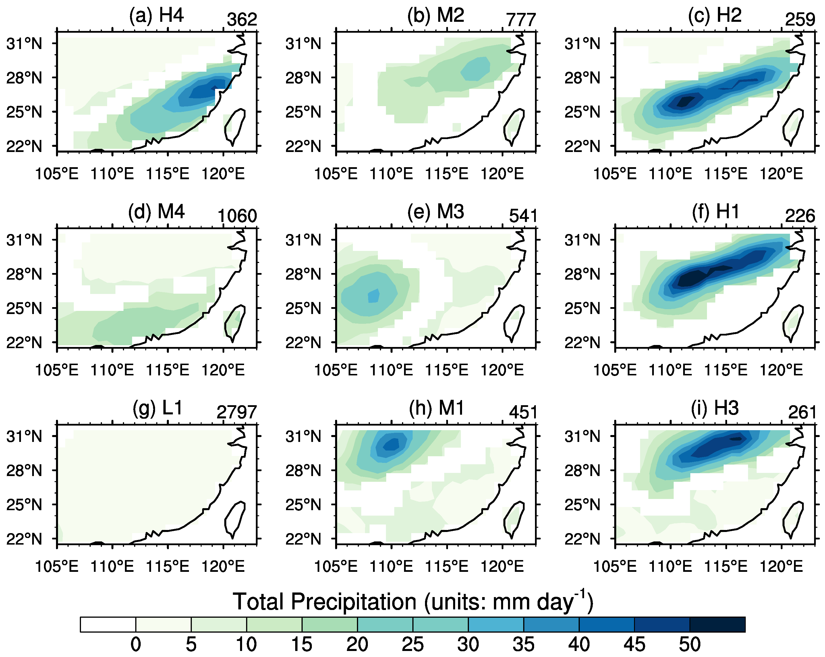
3.1.3. Precipitation Regimes over South China

We applied the SOM clustering method to the ERA-Interim 12-hourly total precipitation over South China (21.5–32° N, 105–123° E) during AMJ 1979–2015. Nine precipitation regimes over South China (Figure 4) are identified from 6734 samples. As shown in Figure 4, obvious distinctions in precipitation amount and spatial pattern exist among the nine precipitation regimes. According to the area-averaged precipitation over South China (${\mathrm{Precip}}_{\mathrm{sc}}$) for the nine regimes, the nine regimes are further classified into three groups: “rainless group” (L-group), “moderate rain group” (M-group), and “heavy rain group” (H-group). Specifically, the criteria of classification are: (1) ${\mathrm{Precip}}_{\mathrm{sc}}$ < 5 mm day⁻¹ for L-group; (2) 5 mm day⁻¹ ≤ ${\mathrm{Precip}}_{\mathrm{sc}}$ < 10 mm day⁻¹ for M-group; and (3) ${\mathrm{Precip}}_{\mathrm{sc}}$ ≥ 10 mm day⁻¹ for H-group. Note that the two thresholds (5 mm day⁻¹ and 10 mm day⁻¹) are adopted mainly for assigning a name to each regime based on the precipitation amounts. However, the results of this paper are insensitive to these two thresholds since the nine regimes (and the associated characteristics including the six factors) are obtained by SOM technique (not based on these two thresholds).

Only one regime (regime L1) belongs to the L-group. The occurrence frequency of L1 is 2797 (accounting for about 41.54% of total samples), which is the most frequent regime among the nine regimes. Under regime L1, South China is short of precipitation (Figure 4g). The sample numbers of regime L1 belonging to April, May, and June are 1164, 952, and 681, respectively. The decrease of the sample number of the rainless regime (i.e., regime L1) with time means that the sample numbers of the regimes with more precipitation increase with time, indicating that the precipitation over South China increases as the summer monsoon season is approaching.

In the M-group, there are four regimes, i.e., M1, M2, M3, and M4. The area-averaged precipitation over South China under these four regimes are 9.62, 9.18, 8.84, and 7.92 mm day⁻¹, respectively, while the corresponding occurrence frequencies are 451 (6.70% of the total), 777 (11.54%), 541 (8.03%), and 1060 (15.74%), respectively. Note that the occurrence frequency of the four M-group regimes (2829 samples; 42.01%) is very close to that of regime L1. The centers of precipitation under these four M-group regimes are rather different. Specifically, the precipitation centers (defined as the location of precipitation maximum under each regime) are located in the northwestern part (around 30° N, 110° E for M1; Figure 4h), northeastern part (around 29° N, 118° E for M2; Figure 4b), western part (around 26° N, 109° E for M3; Figure 4e), and southern part (around 23° N, 113° E for M4; Figure 4d) of South China.

In the H-group, there are four regimes, i.e., H1, H2, H3, and H4. The area-averaged precipitation over South China under these four regimes are 15.55, 14.47, 12.50, and 11.24 mm day⁻¹, respectively, while the corresponding occurrence frequencies are 226 (3.36% of the total), 259 (3.85%), 261 (3.88%), and 362 (5.38%), respectively. Note that the occurrence frequency for each of H-group regimes is lower than any other regime belonging to the M-group or L-group. Therefore, for the nine regimes, the occurrence frequencies basically decrease with precipitation amounts. Each of the four H-group precipitation regimes has a southwest–northeast-orientated horizontal distribution. The centers of precipitation under these four H-group regimes are also different from each other. Specifically, the precipitation centers are located in the central part (around 28° N, 112° E for H1; Figure 4f), central part (around 26° N, 111° E for H2; Figure 4c), northern part (around 31° N, 116° E for H3; Figure 4i), and southeastern part (around 27° N, 119° E for H4; Figure 4a) of South China.

3.2. Dynamic Factors Associated with Different Precipitation Regimes

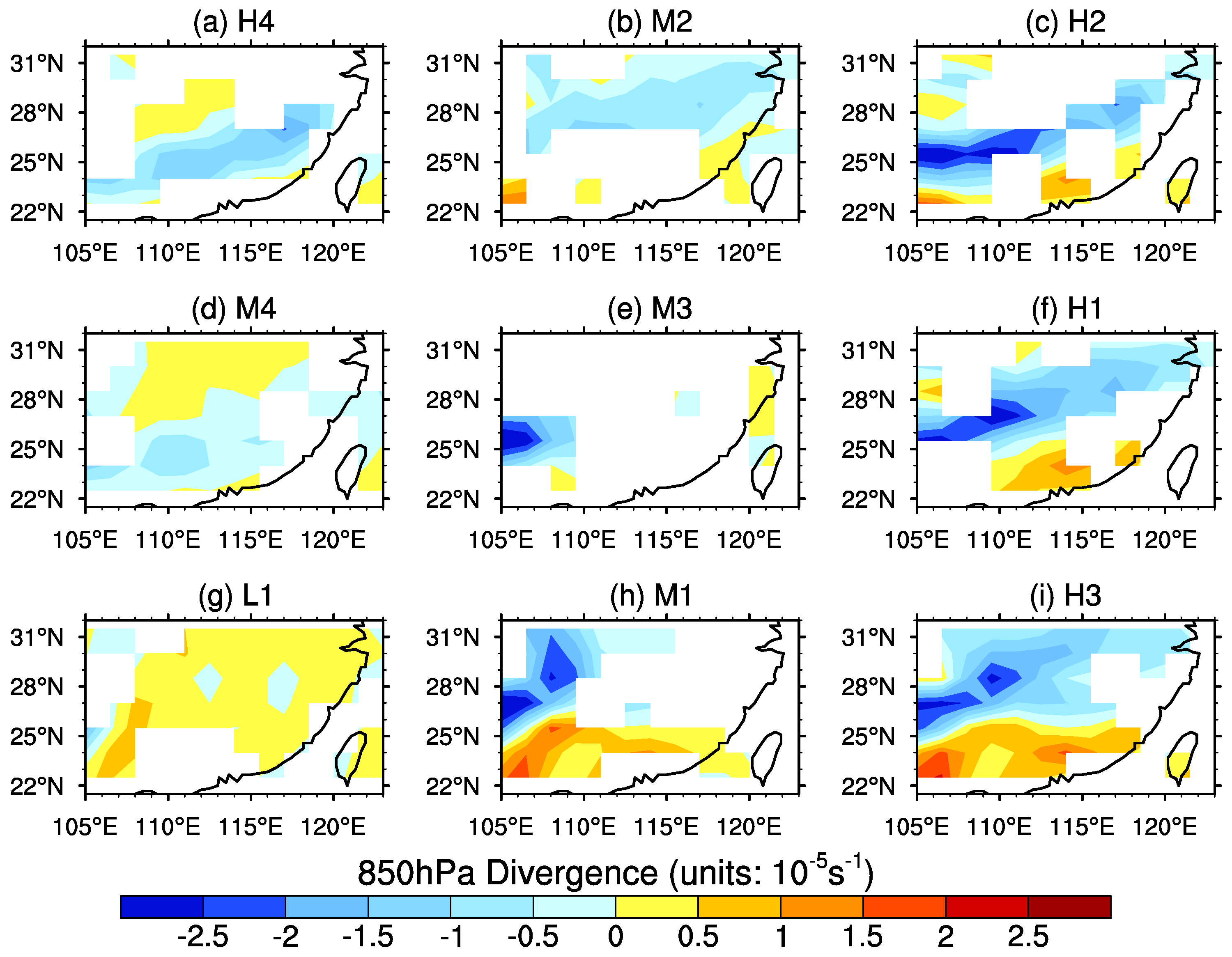
3.2.1. Large-Scale Divergence (Convergence)

Figure 5 and Figure 6 illustrate the horizontal distributions of the composited divergence fields at the 850 hPa and 200 hPa pressure levels for the nine precipitation regimes, respectively. Regime L1, which belongs to the L-group, is characterized by coupling of low-level divergence and high-level convergence (Figure 5g and Figure 6g). The above coupling between low-level and upper-level circulation patterns inhibits the occurrences of precipitation events. Regimes M1 and M3 are characterized by significant low-level convergence in the western part of South China (Figure 5e,h), while regimes M2 and M4 are associated with evident low-level convergence over the northern and southeastern parts of South China (Figure 5b,d), respectively. It should be noted that displacements between centers for low-level convergence and those for precipitation exist under M-group regimes. In addition, although the amplitudes in the low-level convergence under M1 and M3 are larger than those in M2 and M4, the corresponding coverages of the low-level convergence under M1 and M3 are less widespread. Corresponding to the low-level convergence, there is evident divergence in the upper-level (Figure 6b,d,e,h). Compared with the displacements of the low-level convergence, the upper-level divergence are shifted to the northeast and are much more consistent with the locations of precipitation.

The four H-group regimes feature long and narrow bands of low-level convergence (Figure 5a,c,f,i). The coverage of the convergence with amplitudes larger than 1.0 × 10⁻⁵ s⁻¹ is much more widespread than those under other two groups. Compared to the precipitation centers of regimes H1, H2, H3, and H4, the corresponding centers of the low-level convergence are located farther west. By contrast, the geographic positions of the centers for upper-level divergence (Figure 6a,c,f,i) are much more consistent with those for precipitation.

In general, with the exception of L1, all the other precipitation regimes are associated with circulation patterns characterized by coupling of low-level convergence and upper-level divergence. Furthermore, the H-group regimes are associated with stronger upper-level divergence than M-group (the L-group is associated with upper-level convergence), which indicates that the AMJ precipitation over South China may enhance under the background circulation pattern with stronger upper-level divergence.

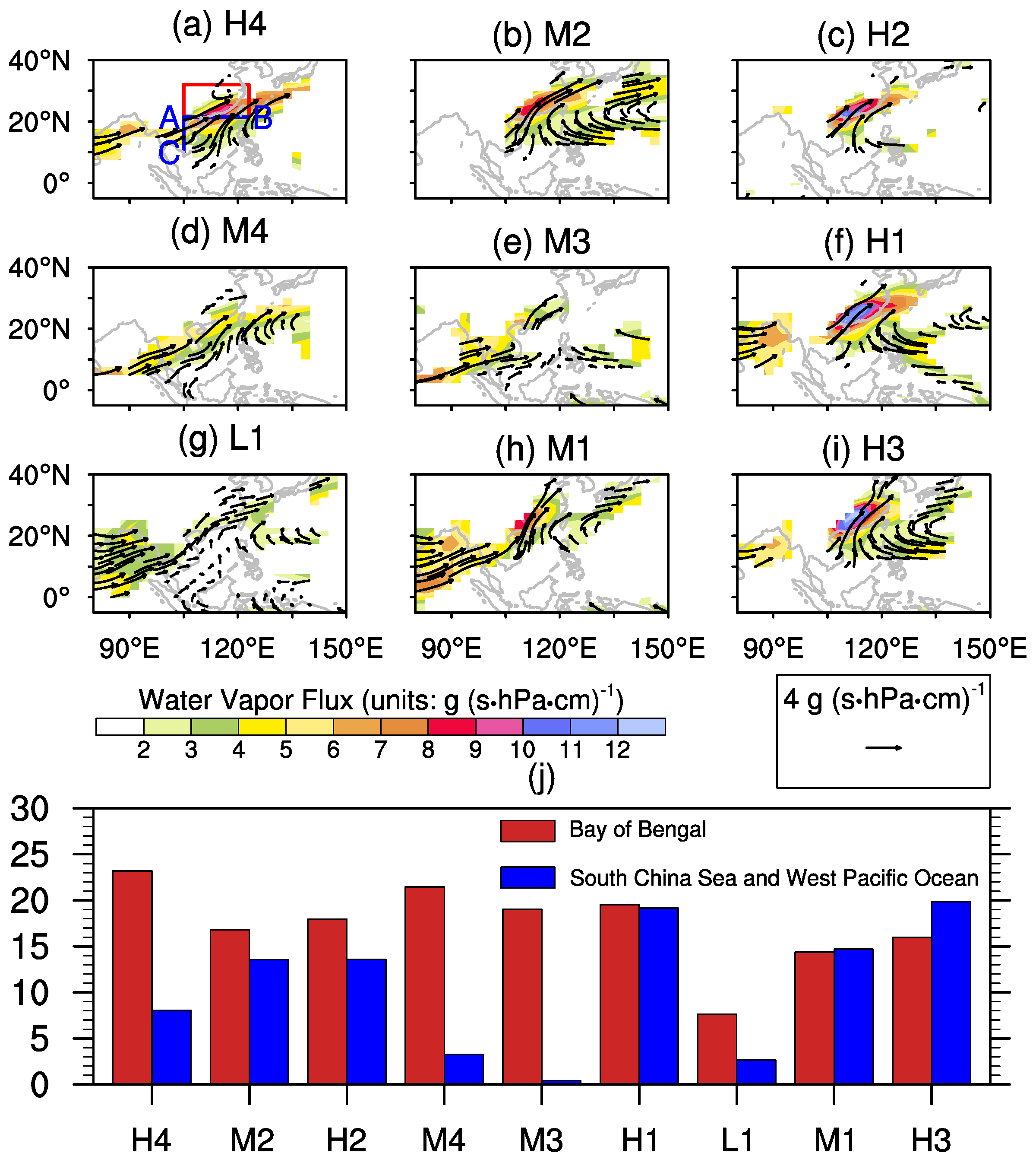
3.2.2. Water Vapor Flux

The water vapor fluxes for the nine regimes estimated based on Equation (2) are illustrated in Figure 7a–i. The centers of water vapor transports in the nine regimes are mainly located over the southeastern coast of South China. Compared to the corresponding precipitation centers, the above centers are shifted to the southeast under most regimes. Besides, the coverage with water vapor transport exceeding 8 g (s·hPa·cm)⁻¹ under the H-group regimes is much more widespread than that under the other two groups, indicating that the water vapor transported into South China under the H-group regimes is more than that under the other two groups.

Based on the estimation of the water vapor transport across the four boundaries of South China, it is revealed that the water vapor over South China is mainly transported from the southern boundary, i.e., the blue line AB (21.5° N, 105–123° E) in Figure 7a. We roughly divide the water vapor transported across the southern boundary of South China into two parts, i.e., water vapor transported from the Bay of Bengal (${\mathrm{T}}_{\mathrm{BoB}}$), and the South China Sea and West Pacific Ocean (${\mathrm{T}}_{\mathrm{SaW}}$). Specifically, ${\mathrm{T}}_{\mathrm{BoB}}$ is estimated as the water vapor across the blue line AC (10–21.5° N, 105° E) in Figure 7a. The southern boundary (i.e., 10° N) is adopted due mainly to the fact that there is no significant water vapor flux in the south of this boundary under any regimes. ${\mathrm{T}}_{\mathrm{SaW}}$ is estimated as the difference between the water vapor across the blue line AB and that across the blue line AC.

Figure 7j displays the ${\mathrm{T}}_{\mathrm{BoB}}$s and ${\mathrm{T}}_{\mathrm{SaW}}$s for the nine regimes. Basically, H-group regimes receive the most water vapor, followed by the M-group regimes, and the regime L1 receives the least water vapor. Therefore, more water vapor transport is favorable for more precipitation during AMJ over South China. Under L1, M3, M4, and H4, the water vapor over South China mainly comes from the Bay of Bengal. By contrast, both the Bay of Bengal and the South China Sea and West Pacific Ocean provide water vapor for the precipitation over South China under M1, M2, H1, H2, and H3. Note that the variation of ${\mathrm{T}}_{\mathrm{BoB}}$s under all the regimes (with the exception of regime L1) is relatively small, which indicates the steadiness of the water vapor transport from the Bay of Bengal. Meanwhile, the South China Sea and West Pacific Ocean mainly provide water vapor for the regimes with more precipitation, i.e., regimes M1, M2, H1, H2, and H3. The above two points indicate that the occurrence probability of more precipitation increases when the water vapor transport from the South China Sea and West Pacific Ocean is enhanced. Similar phenomenon is reported by Simmonds et al. [68] for summer rainfall over southeast China.

3.2.3. Low-Level Jet

Figure 8 illustrates the composite means of winds and their amplitudes on 850 hPa under the nine regimes. The amplitudes of winds for the nine different regimes vary greatly. To capture the variations of low-level jet in the nine regimes, an index for the low-level jet is defined as the area of the winds with amplitudes not less than 8 m s⁻¹ on 850 hPa over South China. The amplitudes of winds over South China under regimes L1, M3, and M4 are all less than 8 m s⁻¹, suggesting that the low-level jet disappears temporarily under these three regimes. The temporary disappearance of the low-level jet can explain the remarkably reduced precipitation under these regimes.

The composite low-level jet indices for the other six regimes are 9.29 × 10⁵ km² (H1), 5.32 × 10⁵ km² (H2), 8.74 × 10⁵ km² (H3), 2.55 × 10⁵ km² (H4), 4.03 × 10⁵ km² (M1), and 3.78 × 10⁵ km² (M2), respectively. The three regimes with remarkably more precipitation, i.e., regimes H1, H2, and H3, are associated with the three strongest low-level jets. The centers of low-level jets under the above six regimes are located over the southwest of precipitation centers, indicating that the location of precipitation is mainly modulated by the direction of low-level jet. Take regimes H1, H2, and H3 as examples. Among these three regimes, the regime (H3) with the northernmost low-level jet is associated with the northernmost precipitation center, while the regime (H2) with the southernmost low-level jet is associated with the southernmost precipitation center.

The above analysis about the low-level jet is consistent with that about the transport of water vapor. Specifically, more water vapor is provided by stronger low-level jet, and the direction of low-level jet affects the position where water vapor can be transported to and further modulates the precipitation center.

3.3. Thermodynamic Factors Associated with Different Precipitation Regimes

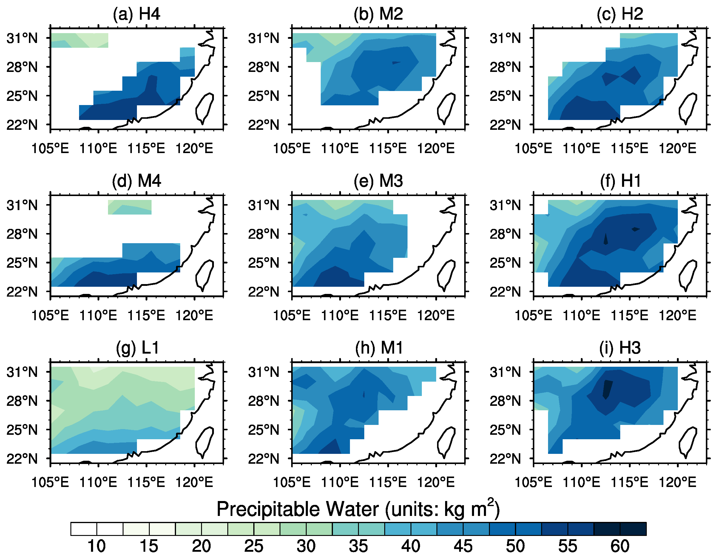
3.3.1. Precipitable Water

Figure 9 displays the horizontal distributions of composite precipitable water under the nine regimes. Basically, the precipitable water over South China decreases with the latitude, which can be understood by the following two points. First, the air temperature decreases with the latitude over South China. Second, air mass with higher temperature is capable of storing more water vapor. However, there are some exceptions. Under regimes H1, H2, H3, and M2, there are localized maxima of precipitable water near 28° N (Figure 9b,c,f,i). The occurrence of localized maxima is mainly due to the following two aspects. First, during the preparatory stage of the precipitation under these four regimes, the localized heat source is in favor of the moistening lower troposphere and further increases the precipitable water. Second, the powerful low-level jets under these four regimes are able to transport abundant water vapor into these regions which are far away from the coasts.

To quantitatively explore the relationship between precipitation and precipitable water, we calculate the area-averaged precipitable water under each regime. The area-averaged precipitable water for the nine regimes are 33.18 kg m² (L1), 40.67 kg m² (M4), 42.81 kg m² (M3), 43.43 kg m² (M2), 44.84 kg m² (M1), 41.83 kg m² (H4), 46.55 kg m² (H3), 43.47 kg m² (H2), and 46.87 kg m² (H1). Basically, the regime with more precipitable water is inclined to be associated with more precipitation. However, the above relationship is not strictly monotonic. Specifically, the regime with second largest precipitation (H2) over South China has less precipitable water than the regime with third largest precipitation (H3) and an M-group regime (M1). In addition, the regime with fourth largest precipitation (H4) over South China has less precipitable water than almost all M-group regimes (M1–M3). Therefore, more precipitable water is not a necessary condition for forming more severe precipitation.

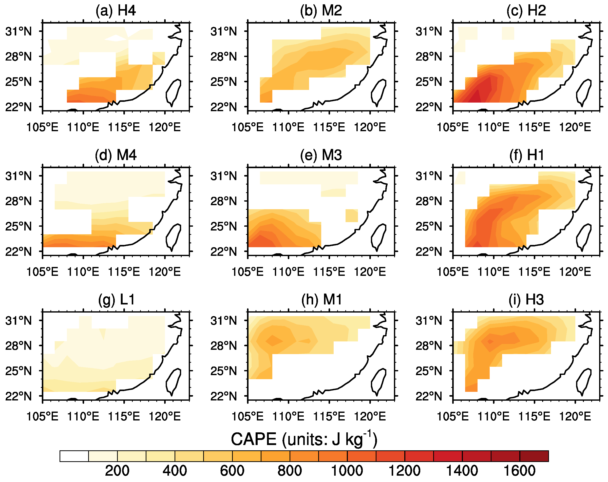
3.3.2. Convective Available Potential Energy

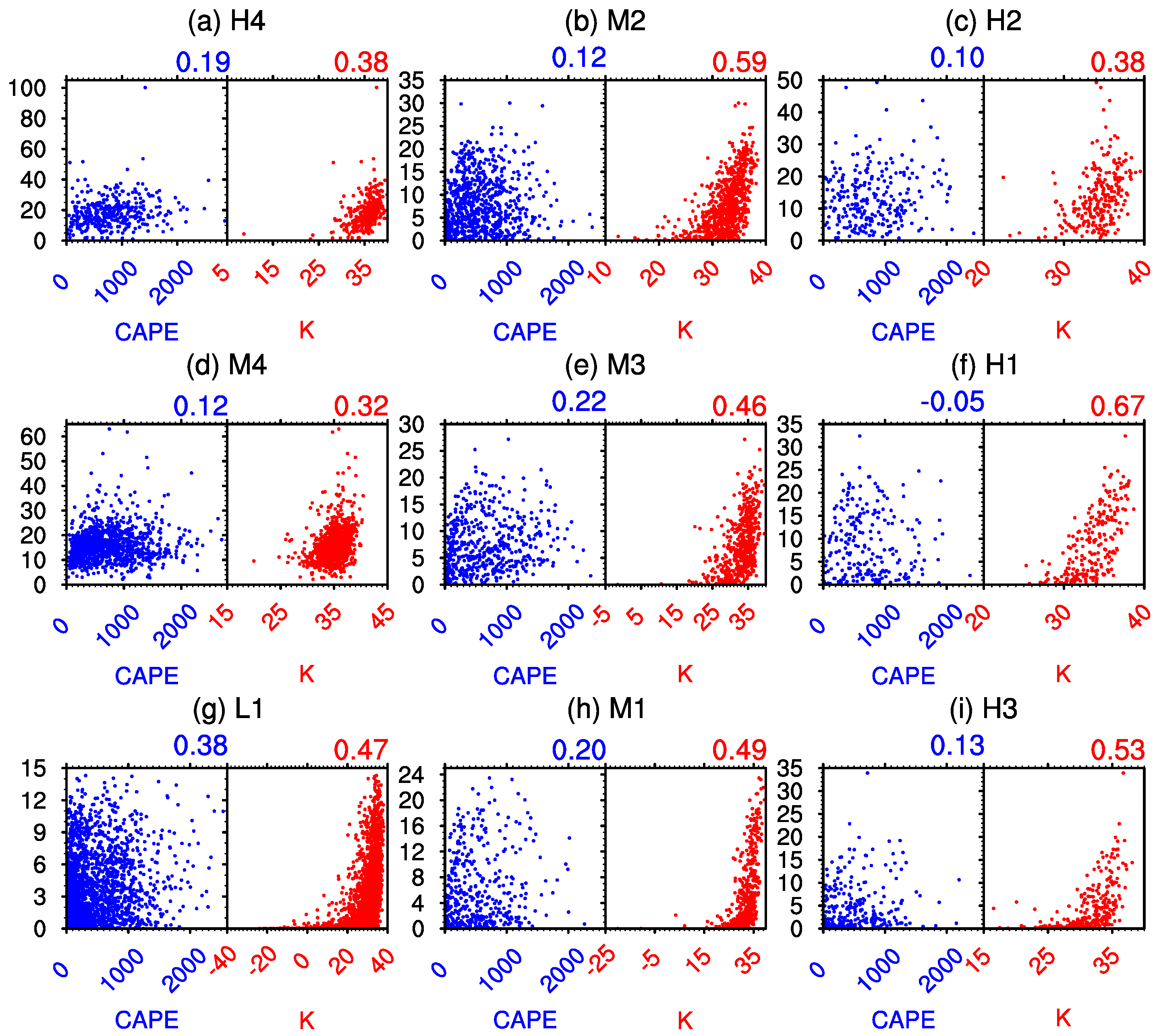
The composite means of CAPE under the nine regimes are shown in Figure 10. The maximum CAPE over South China under regime L1 is less than 500 J kg⁻¹ (Figure 10g), indicating that the convective instability is very weak and thus the probability of convective precipitation is remarkably reduced. The maxima of CAPE under the H-group regimes are 1176.11 J kg⁻¹ (H1), 1391.96 J kg⁻¹ (H2), 930.72 J kg⁻¹ (H3), and 1046.93 J kg⁻¹ (H4), respectively. The threshold in CAPE for the moderate convective instability is 1000 J kg⁻¹ [69], which indicates that the convective instability under regime H3 is still in a weak level. Note that regime H2 has much larger convective instability but less precipitation than regime H1, which can be explained by its weaker low-level jet (Section 3.2.3). The maximum in CAPE under each of the H-group regimes is located at the southwest of the corresponding precipitation center (Figure 10a,c,f,i). The maxima in CAPE for two M-group regimes, i.e., regimes M1 and M3, are also located at the southwest of the corresponding precipitation centers (Figure 10e,h). However, the maxima in CAPE for another two M-group regimes, i.e., regimes M2 and M4, are located at the west of the corresponding precipitation centers (Figure 10b,d). The corresponding maxima of CAPE under the M-group regimes are 740.26 J kg⁻¹ (M1), 819.06 J kg⁻¹ (M2), 1068.11 J kg⁻¹ (M3), and 989.17 J kg⁻¹ (M4), respectively. Regime M3 has the largest convective instability among the M-group regimes but less precipitation than regimes M1 and M2, which can be explained by the temporary disappearance of low-level jet under this regime.

The staggered placements between maxima in CAPE and precipitation centers under the nine regimes can be explained by the following three aspects. First, the stratiform precipitation is as important as the convective precipitation during AMJ over South China. Second, the supply of sufficient water vapor to the region with strong convective instability is the necessary condition for forming the convective precipitation. Therefore, the lack of favorable large-scale conditions (e.g., the low-level jet) will also lead to the staggered placements. Third, as the timescale of convective precipitation is usually less than three hours, the use of 12-hourly analysis frequency may introduce the observed displacements.

3.3.3. K Index

Figure 11 illustrates the composite means of K index under nine regimes. The eight regimes belonging to the M-group and H-group have widespread areas with K index exceeding 30. As pointed by Dalezios and Papamanolis [70], the occurrence probability of severe convection is extremely high when the local K index is larger than 30.

Under the two regimes with the most and second most precipitation, i.e., regimes H1 and H2, the maxima in K index are very close to the precipitation center (Figure 11c,f). Under the other two H-group regimes, i.e., regimes H3 and H4, the maxima in K index are shifted to the southwest of precipitation centers (Figure 11a,i), which is similar to the maxima in CAPE. However, compared with the maxima in CAPE, the maxima in K index are slightly closer to the precipitation centers under H3 and H4.

Under M-group regimes, the maxima of K index are also located at the southwest of the corresponding precipitation centers (Figure 11b,d,e,h). Likewise, the distances between the maxima in K index and the corresponding precipitation centers are a bit shorter than the distances between the maxima in CAPE and the corresponding precipitation centers.

3.3.4. A Further Comparison between CAPE and K Index

This section is devoted to making a further comparison between the CAPE and K index in terms of their relationships with the area-averaged precipitation. Considering the fact that the area average over the whole South China inevitably leads to offsets among the local instabilities belonging to different regions, the comparison here takes Guangdong Province (21.5–25° N, 109–117° E) as an example.

Figure 12 shows the relationship between area-averaged precipitation and these two indices over Guangdong Province under all the regimes. The correlation coefficients between area-averaged precipitation and CAPE do not exceed 0.22 for all the regimes with the exception of regime L1 (0.38), indicating that the relationship between precipitation and CAPE is rather complicated. By contrast, K index has a closer relationship with precipitation. Specifically, the corresponding correlation coefficients between area-averaged K index and precipitation for the nine regimes are 0.47 (L1), 0.32 (M4), 0.46 (M3), 0.59 (M2), 0.49 (M1), 0.38 (H4), 0.53 (H3), 0.38 (H2), and 0.67 (H1), which are significantly larger than those between the area-averaged CAPE and precipitation. Similar studies for the other coastal provinces over South China also confirm that K index has a closer relationship with precipitation than CAPE during AMJ. Combining the analysis in above two sections, it is inferred that K index is a better thermodynamic indicator for AMJ precipitation over South China.

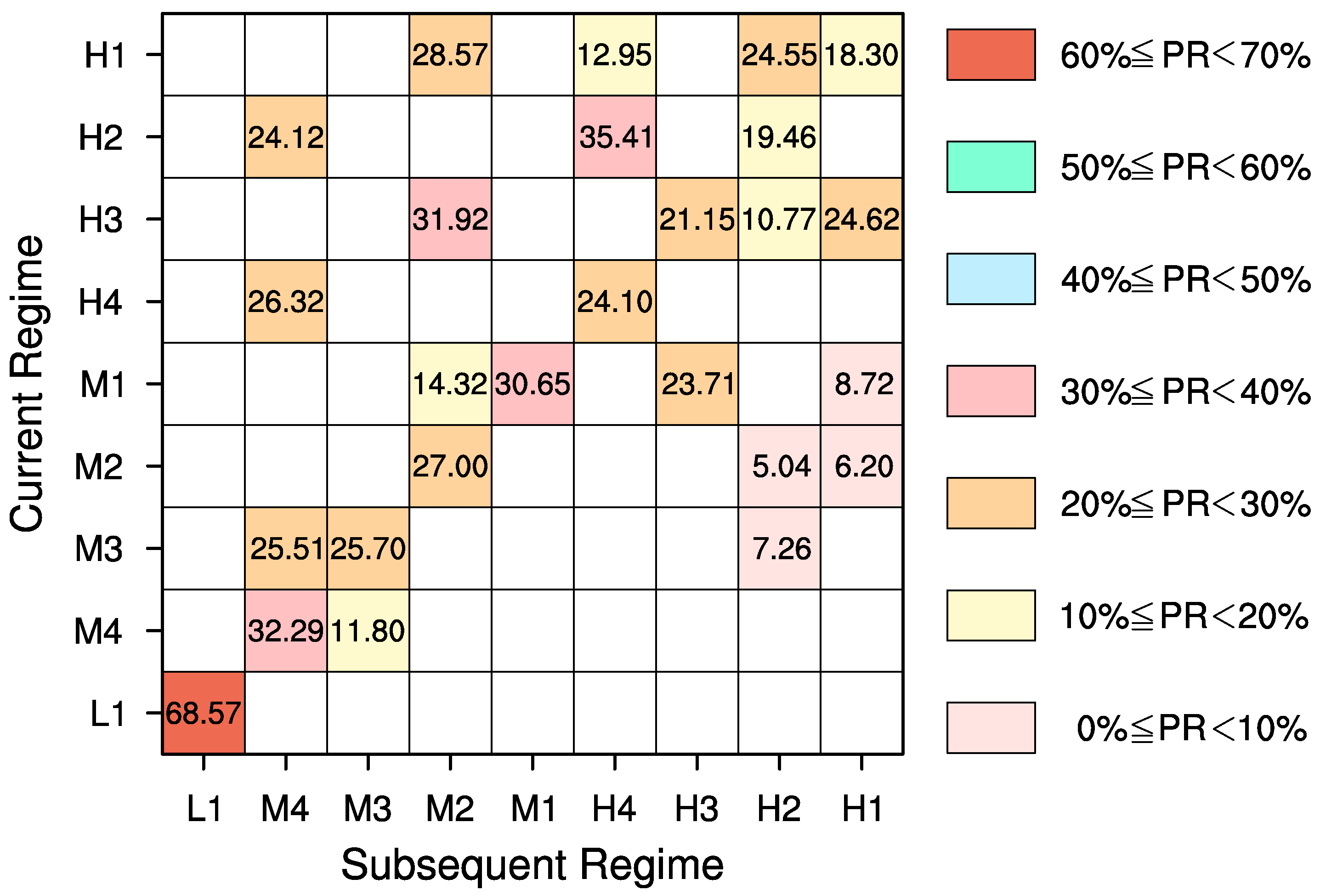
3.4. Persistence and Transformations of the Precipitation Regimes

This section is devoted to analyzing the persistence and transformation probabilities for the nine different precipitation regimes. The persistence probability for a specific regime is estimated as the ratio of samples belonging to the same regime for which the following sample belongs to the same regime. Likewise, the transformation probability between two different regimes is estimated as the ratio of samples belonging to the first regime for which the following sample belongs to the second regime. After Espinoza et al. [71] and Huang et al. [36], the statistical significance of a persistence/transformation is tested as follows. First, randomly permute the sequence of precipitation regime types for the 6734 samples during AMJ 1979–2015 1000 times. Second, calculate the persistence and transformation probabilities for the randomly-permuted 1000 sequences of precipitation regime types. Third, the 95th percentile of the 1000 corresponding probabilities is identified as the threshold. Finally, a persistence/transformation is viewed as statistically significant when the corresponding probability is not less than the identified threshold.

Figure 13 shows the probabilities for the significant persistence and transformations. The persistence probabilities for the nine regimes range from 18.30% (H1) to 68.57% (L1). Besides, the persistence probability generally decreases with the precipitation amount for all the regimes except M2 and M3. The persistence probability for each of the nine regimes (with the exception of regime L1) is less than the transformation probabilities to the other regimes.

Table 1. The subsequent regimes that a current regime (the leftmost column) transforms into with statistical significance. The associated features of the subsequent regime relative to the current regime are shown in the parenthesis (“L”/“M” represents that the subsequent regime rains less/more relative to the current regime, while “S”/“N” represents that the precipitation center for the subsequent regime is located in south/north of that for the current regime).

Current Regime	Subsequent Regimes
L1
M4	M3 (M; N)
M3	M4 (L; S)	H2 (M; S)
M2	H2 (M; S)	H1 (M)
M1	M2 (L; S)	H3 (M; S)	H1 (M; S)
H4	M4 (L; S)
H3	M2 (L; S)	H2 (M; S)	H1 (M; S)
H2	M4 (L; S)	H4 (L; S)
H1	M2 (L)	H4 (L; S)	H2 (L; S)

further summarizes the characteristics of transformations associated with each regime. The transformations generally feature southward shifts of the precipitation centers. The above characteristic can be explained by the consumption of water vapor during the precipitation, which results in the southward shift of the precipitation center to the area with sufficient water vapor.

3.5. Heavy Precipitation Events

In this section, the characteristics of heavy precipitation events over South China during AMJ are analyzed from the perspective of precipitation regimes. A heavy precipitation event is identified when the precipitation with a rate of 10 mm 12 h⁻¹ lasts for at least 12 h. Note that the criterion of a heavy precipitation event is different from that of H-group regimes for which the threshold is 10 mm day⁻¹. A heavy precipitation event lasting for at least 24 h is viewed as a persistent heavy precipitation event. Totally, 50 heavy precipitation events (69 samples) and 15 persistent heavy precipitation events are identified. The number of samples for heavy precipitation events under the nine regimes are thirty (H1), nineteen (H2), nine (H3), four (H4), five (M1), one (M2), nine (M3), one (M4), and zero (L1), conforming that regimes H1 and H2 are the major regimes for the heavy precipitation events and further demonstrating the reasonability of identifying precipitation regimes based on the SOM technique.

Among the 15 persistent heavy precipitation events, 11 events are associated with regime transformations. All the 11 regime transformations feature distinct southward shifts of precipitation centers, which is consistent with the transformation characteristics between different regimes as revealed in the previous section. Besides, it is worth noting that the most preferred target regimes for the 11 regime transformations are regimes H1 (six among eleven) and H2 (three among eleven).

Based on the above sections, the major findings of our study are concluded and shown in Figure 14.

4. Conclusions

By applying the SOM clustering technique to the sub-daily precipitation during pre-monsoon season (AMJ) of 1979–2015, nine precipitation regimes over South China are obtained. The nine regimes differ from each other in terms of their precipitation amounts, spatial patterns, and occurrence frequencies. According to the precipitation amounts, the nine regimes are further classified into three groups: the L-group (one regime), M-group (four regimes), and H-group (four regimes).

The relationships between different regimes and dynamic/thermodynamic factors are explored. The dynamic factors include the large-scale divergence (convergence), water vapor flux, and low-level jet, while the thermodynamic factors include the precipitable water, CAPE, and K index. Among the six factors, the upper-level divergence is the best indicator for the geographic positions of precipitation centers, and more precipitation occurs under the background with stronger upper-level divergence. Besides, the geographic positions of precipitation centers are also modulated by the directions of low-level jets. Based on the estimation of the water vapor transport across the four boundaries of South China, it is revealed that the water vapor over South China is mainly transported from the southern boundary. Further estimation reveals that the Bay of Bengal provides water vapor for all the nine regimes, while the South China Sea and West Pacific Ocean provide water vapor for five regimes. More water vapor transport is favorable for more precipitation, and the water vapor supporting the more precipitation is mainly from the South China Sea and West Pacific Ocean. K index is a better thermodynamic indicator for the precipitation over South China than CAPE in terms of their relationships with area-averaged precipitation amounts and spatial patterns of precipitation. Compared to the other five factors, the precipitable water performs worse in capturing the characteristics of precipitation over South China. Furthermore, the persistence and transformations among the nine precipitation regimes are analyzed. It is revealed that the regimes with more precipitation have lower persistence probabilities. The low-level jet stream tends to be weakened after the heavy precipitation, resulting in that the moisture transported by the low-level jet could only be delivered to a relative south location. Consequently, the regime transformations are always associated with southward shifts in the precipitation centers.

Although the nine precipitation regimes are obtained based on the ERA-Interim precipitation data, a composite analysis of these nine precipitation regimes based on the precipitation data from surface stations confirms the reliability of these regimes in terms of both the horizontal distributions and intensities (Figure 15). It should be noted that this study only explored three dynamics factors and three thermodynamic factors associated with each of the nine precipitation regimes during AMJ 1979–2015. More analyses, especially the evolution characteristics of the dynamic and thermodynamic factors before these precipitation regimes, are needed to propose possible formation mechanisms. In addition, further analyses about other factors are also beneficial for improving our understanding of these precipitation regimes. For example, we may also include the factor relative humidity, which tends to be higher in the regimes with more precipitation than those in the regimes with less precipitation (Figure 16).

The transformation characteristics of the precipitation regimes shown in this study can be used to predict the future evolution of the horizontal distribution (especially the precipitation center) of the precipitation after heavy precipitation events. The finding that the K index has an advantage in indicating the precipitation center over the CAPE may benefit not only routine weather prediction, but also other future studies that focus on the convection precipitation. Besides, due primarily to the fact that the precipitation is always associated with different horizontal distributions and intensities, exploring the characteristics of the precipitation using the SOM technique can be applied to the future studies about the precipitation over different regions or different seasons.

References

1. Ding, Y.; Wang, Z. A study of rainy seasons in China. Meteorol. Atmos. Phys. 2008, 100, 121–138. [Google Scholar]
2. Gu, W.; Wang, L.; Hu, Z.; Hu, K.; Li, Y. Interannual Variations of the First Rainy Season Precipitation over South China. J. Clim. 2018, 31, 623–640. [Google Scholar] [CrossRef]
3. Wu, X.; Mao, J. Interdecadal modulation of ENSO-related spring rainfall over South China by the Pacific Decadal Oscillation. Clim. Dyn. 2016, 47, 3203–3220. [Google Scholar] [CrossRef]
4. Yang, F.; Lau, K. Trend and variability of China precipitation in spring and summer: Linkage to sea-surface temperatures. Int. J. Climatol. 2004, 24, 1625–1644. [Google Scholar] [CrossRef]
5. Sun, J.; Zhao, S. A diagnosis and simulation study of a strong heavy rainfall in South China. Chin. J. Atmos. Sci. 2000, 24, 381–392. [Google Scholar]
6. Chan, J.C.L.; Zhou, W. PDO, ENSO and the early summer monsoon rainfall over south China. Geophys. Res. Lett. 2005, 32, L08810. [Google Scholar] [CrossRef]
7. Ding, Y.; Wang, Z.; Sun, Y. Inter-decadal variation of the summer precipitation in East China and its association with decreasing Asian summer monsoon. Part I: Observed evidences. Int. J. Climatol. 2008, 28, 1139–1161. [Google Scholar] [CrossRef]
8. Ding, Y.; Sun, Y.; Wang, Z.; Zhu, Y.; Song, Y. Inter-decadal variation of the summer precipitation in China and its association with decreasing Asian summer monsoon Part II: Possible causes. Int. J. Climatol. 2009, 29, 1926–1944. [Google Scholar] [CrossRef] [Green Version]
9. Yuan, W.; Yu, R.; Chen, H.; Li, J.; Zhang, M. Subseasonal Characteristics of Diurnal Variation in Summer Monsoon Rainfall over Central Eastern China. J. Clim. 2010, 23, 6684–6695. [Google Scholar] [CrossRef]
10. Hu, K.; Huang, G. The Formation of Precipitation Anomaly Patterns during the Developing and Decaying Phases of ENSO. Atmos. Ocean. Sci. Lett. 2010, 3, 25–30. [Google Scholar]
11. Mao, J.; Chan, J.C.L.; Wu, G. Interannual variations of early summer monsoon rainfall over South China under different PDO backgrounds. Int. J. Climatol. 2011, 31, 847–862. [Google Scholar] [CrossRef] [Green Version]
12. Mao, J.; Wu, G. Diurnal variations of summer precipitation over the Asian monsoon region as revealed by TRMM satellite data. Sci. China Earth Sci. 2012, 55, 554–566. [Google Scholar] [CrossRef]
13. Yuan, W.; Yu, R.; Zhang, M.; Lin, W.; Li, J.; Fu, Y. Diurnal Cycle of Summer Precipitation over Subtropical East Asia in CAM5. J. Clim. 2013, 26, 3159–3172. [Google Scholar] [CrossRef]
14. Wang, L.; Gu, W. The Eastern China flood of June 2015 and its causes. Sci. Bull. 2016, 61, 178–184. [Google Scholar] [CrossRef]
15. Ao, J.; Sun, J. Decadal change in factors affecting winter precipitation over eastern China. Clim. Dyn. 2016, 46, 111–121. [Google Scholar] [CrossRef]
16. Ao, J.; Sun, J. The impact of boreal autumn SST anomalies over the South Pacific on boreal winter precipitation over East Asia. Adv. Atmos. Sci. 2016, 33, 644–655. [Google Scholar] [CrossRef]
17. Ge, J.; Jia, X.; Lin, H. The interdecadal change of the leading mode of the winter precipitation over China. Clim. Dyn. 2016, 47, 2397–2411. [Google Scholar] [CrossRef]
18. Jia, X.; Ge, J. Interdecadal Changes in the Relationship between ENSO, EAWM, and the Wintertime Precipitation over China at the End of the Twentieth Century. J. Clim. 2017, 30, 1923–1937. [Google Scholar] [CrossRef]
19. Zhao, S.; Bei, N.; Sun, J. Mesoscale analysis of a heavy rainfall event over Hong Kong during a pre-rainy season in South China. Adv. Atmos. Sci. 2007, 24, 555–572. [Google Scholar] [CrossRef]
20. Chen, C.; Lin, K.; Wang, P. Relation between Pre-flood Season Precipitation Anomalies in South China and Water Vapor Transportation. J. Nanjing Inst. Meteorol. 2004, 27, 721–727. [Google Scholar]
21. Trenberth, K.E.; Dai, A.; Rasmussen, R.M.; Parsons, D.B. The Changing Character of Precipitation. Bull. Am. Meteorol. Soc. 2003, 84, 1205–1217. [Google Scholar] [CrossRef]
22. Birk, K.; Lupo, A.R.; Guinan, P.; Barbieri, C.E. The interannual variability of midwestern temperatures and precipitation as related to the ENSO and PDO. Atmósfera 2010, 23, 95–128. [Google Scholar]
23. Nunes, M.J.; Lupo, A.R.; Lebedeva, M.G.; Chendev, Y.G.; Solovyov, A.B. The Occurrence of Extreme Monthly Temperatures and Precipitation in Two Global Regions. Pap. Appl. Geogr. 2017, 3, 143–156. [Google Scholar] [CrossRef]
24. Rabinowitz, J.L.; Lupo, A.R.; Guinan, P.E. Evaluating Linkages between Atmospheric Blocking Patterns and Heavy Rainfall Events across the North-Central Mississippi River Valley for Different ENSO Phases. Adv. Meteorol. 2018, 2018, 1217830. [Google Scholar] [CrossRef]
25. Kohonen, T. Self-organized formation of topologically correct feature maps. Biol. Cybern. 1982, 43, 59–69. [Google Scholar] [CrossRef]
26. Cavazos, T. Using Self-Organizing Maps to Investigate Extreme Climate Events: An Application to Wintertime Precipitation in the Balkans. J. Clim. 2000, 13, 1718–1732. [Google Scholar] [CrossRef]
27. Crimmins, M.A. Synoptic climatology of extreme fire-weather conditions across the southwest United States. Int. J. Climatol. 2006, 26, 1001–1016. [Google Scholar] [CrossRef] [Green Version]
28. Nishiyama, K.; Endo, S.; Jinno, K.; Uvo, C.B.; Olsson, J.; Berndtsson, R. Identification of typical synoptic patterns causing heavy rainfall in the rainy season in Japan by a Self-Organizing Map. Atmos. Res. 2007, 83, 185–200. [Google Scholar] [CrossRef]
29. Brown, J.R.; Jakob, C.; Haynes, J.M. An Evaluation of Rainfall Frequency and Intensity over the Australian Region in a Global Climate Model. J. Clim. 2010, 23, 6504–6525. [Google Scholar] [CrossRef] [Green Version]
30. Cassano, E.N.; Cassano, J.J. Synoptic forcing of precipitation in the Mackenzie and Yukon River basins. Int. J. Climatol. 2010, 30, 658–674. [Google Scholar] [CrossRef]
31. Sheridan, S.C.; Lee, C.C. The self-organizing map in synoptic climatological research. Prog. Phys. Geogr. 2011, 35, 109–119. [Google Scholar] [CrossRef]
32. Huang, W.; Chen, R.; Yang, Z.; Wang, B.; Ma, W. Exploring the combined effects of the Arctic Oscillation and ENSO on the wintertime climate over East Asia using self-organizing maps. J. Geophys. Res. Atmos. 2017, 122, 9107–9129. [Google Scholar] [CrossRef]
33. Chen, R.; Huang, W.; Wang, B.; Yang, Z.; Wright, J.S.; Ma, W. On the cooccurrence of wintertime temperature anomalies over eastern Asia and eastern North America. J. Geophys. Res. Atmos. 2017, 122, 6844–6867. [Google Scholar] [CrossRef]
34. Schuenemann, K.C.; Cassano, J.J.; Finnis, J. Synoptic Forcing of Precipitation over Greenland: Climatology for 1961–99. J. Hydrometeorol. 2009, 10, 60–78. [Google Scholar] [CrossRef]
35. Polo, I.; Ullmann, A.; Roucou, P.; Fontaine, B. Weather Regimes in the Euro-Atlantic and Mediterranean Sector, and Relationship with West African Rainfall over the 1989–2008 Period from a Self-Organizing Maps Approach. J. Clim. 2011, 24, 3423–3432. [Google Scholar] [CrossRef] [Green Version]
36. Huang, W.; Chen, R.; Wang, B.; Wright, J.S.; Yang, Z.; Ma, W. Potential vorticity regimes over East Asia during winter. J. Geophys. Res. Atmos. 2017, 122, 1524–1544. [Google Scholar] [CrossRef]
37. Li, R.C.Y.; Zhou, W. Multiscale control of summertime persistent heavy precipitation events over South China in association with synoptic, intraseasonal, and low-frequency background. Clim. Dyn. 2015, 45, 1043–1057. [Google Scholar] [CrossRef]
38. Hong, W.; Ren, X. Persistent heavy rainfall over South China during May–August: Subseasonal anomalies of circulation and sea surface temperature. Acta Meteorol. Sin. 2013, 27, 769–787. [Google Scholar] [CrossRef]
39. Chen, Y.; Zhai, P. Persistent extreme precipitation events in China during 1951-2010. Clim. Res. 2013, 57, 143–155. [Google Scholar] [CrossRef]
40. Dee, D.P.; Uppala, S.M.; Simmons, A.J.; Berrisford, P.; Poli, P.; Kobayashi, S.; Andrae, U.; Balmaseda, M.A.; Balsamo, G.; Bauer, P.; et al. The ERA-Interim reanalysis: configuration and performance of the data assimilation system. Q. J. R. Meteorol. Soc. 2011, 137, 553–597. [Google Scholar] [CrossRef] [Green Version]
41. Becker, A.; Finger, P.; Meyer-Christoffer, A.; Rudolf, B.; Schamm, K.; Schneider, U.; Ziese, M. A description of the global land-surface precipitation data products of the Global Precipitation Climatology Centre with sample applications including centennial (trend) analysis from 1901-present. Earth Syst. Sci. Data 2013, 5, 71–99. [Google Scholar] [CrossRef]
42. Ohba, M.; Kadokura, S.; Yoshida, Y.; Nohara, D.; Toyoda, Y. Anomalous Weather Patterns in Relation to Heavy Precipitation Events in Japan during the Baiu Season. J. Hydrometeorol. 2015, 16, 688–701. [Google Scholar] [CrossRef]
43. Reusch, D.B.; Alley, R.B.; Hewitson, B.C. North Atlantic climate variability from a self-organizing map perspective. J. Geophys. Res. Atmos. 2007, 112, D02104. [Google Scholar] [CrossRef]
44. Leloup, J.A.; Lachkar, Z.; Boulanger, J.P.; Thiria, S. Detecting decadal changes in ENSO using neural networks. Clim. Dyn. 2007, 28, 147–162. [Google Scholar] [CrossRef]
45. Herbst, M.; Casper, M.C. Towards model evaluation and identification using Self-Organizing Maps. Hydrol. Earth Syst. Sci. 2008, 12, 657–667. [Google Scholar] [CrossRef] [Green Version]
46. Ciampi, A.; Lechevallier, Y. Clustering Large, Multi-level Data Sets: An Approach Based on Kohonen Self Organizing Maps. In Principles of Data Mining and Knowledge Discovery; Zighed, D.A., Komorowski, J., Żytkow, J., Eds.; Springer: Berlin, Heidelberg, 2000; pp. 353–358. [Google Scholar]
47. Zhang, R. Relations of Water Vapor Transport from Indian Monsoon with that over East Asia and the Summer Rainfall in China. Adv. Atmos. Sci. 2001, 18, 1005–1017. [Google Scholar]
48. Feng, L.; Zhou, T. Water vapor transport for summer precipitation over the Tibetan Plateau: Multidata set analysis. J. Geophys. Res. Atmos. 2012, 117, D20114. [Google Scholar] [CrossRef]
49. He, M.; Liu, H.; Wang, B.; Zhang, D. A Modeling Study of a Low-Level Jet along the Yun-Gui Plateau in South China. J. Appl. Meteorol. Climatol. 2016, 55, 41–60. [Google Scholar] [CrossRef]
50. Qian, J.; Tao, W.; Lau, K.M. Mechanisms for Torrential Rain Associated with the Mei-Yu Development during SCSMEX 1998. Mon. Weather Rev. 2004, 132, 3–27. [Google Scholar] [CrossRef]
51. Higgins, R.W.; Yao, Y.; Yarosh, E.S.; Janowiak, J.E.; Mo, K.C. Influence of the Great Plains Low-Level Jet on Summertime Precipitation and Moisture Transport over the Central United States. J. Clim. 1997, 10, 481–507. [Google Scholar] [CrossRef]
52. Jiang, J.; Jiang, J.; Bu, Y.; Liu, N. Heavy Rainfall Associated with a Monsoon Depression in South China: Structure Analysis. J. Meteorol. Res. 2008, 22, 53–67. [Google Scholar]
53. Bonner, W.D. Climatology of the low level jet. Mon. Weather Rev. 1968, 96, 833–850. [Google Scholar] [CrossRef]
54. Liu, H.; Li, L.; Wang, B. Low-Level Jets over Southeast China: The Warm Season Climatology of the Summer of 2003. Atmos. Ocean. Sci. Lett. 2012, 5, 394–400. [Google Scholar]
55. Zhang, R.; Sumi, A. Moisture Circulation over East Asia during El Niño Episode in Northern Winter, Spring and Autumn. J. Meteorol. Soc. Jpn. 2002, 80, 213–227. [Google Scholar] [CrossRef]
56. Zhai, P.; Eskridge, R.E. Atmospheric Water Vapor over China. J. Clim. 1997, 10, 2643–2652. [Google Scholar] [CrossRef]
57. Kastman, J.S.; Market, P.S.; Fox, N.I.; Foscato, A.L.; Lupo, A.R. Lightning and Rainfall Characteristics in Elevated vs. Surface Based Convection in the Midwest that Produce Heavy Rainfall. Atmosphere 2017, 8, 36. [Google Scholar] [CrossRef]
58. Doswell, C.A.; Rasmussen, E.N. The Effect of Neglecting the Virtual Temperature Correction on CAPE Calculations. Weather Forecast. 1994, 9, 625–629. [Google Scholar] [CrossRef] [Green Version]
59. Blanchard, D.O. Assessing the Vertical Distribution of Convective Available Potential Energy. Weather Forecast. 1998, 13, 870–877. [Google Scholar] [CrossRef] [Green Version]
60. Barkiđija, S.; Fuchs, Ž. Precipitation correlation between convective available potential energy, convective inhibition and saturation fraction in middle latitudes. Atmos. Res. 2013, 124, 170–180. [Google Scholar] [CrossRef]
61. Riemann-Campe, K.; Fraedrich, K.; Lunkeit, F. Global climatology of Convective Available Potential Energy (CAPE) and Convective Inhibition (CIN) in ERA-40 reanalysis. Atmos. Res. 2009, 93, 534–545. [Google Scholar] [CrossRef]
62. Charba, J.P. Operational System for Predicting Thunderstorms Two to Six Hours in Advance; NOAA Technical Memorandum NWS TDL-64; National Oceanic and Atmospheric Administration: Silver Spring, MD, USA, 1977.
63. Duchon, C.E. Lanczos Filtering in One and Two Dimensions. J. Appl. Meteorol. 1979, 18, 1016–1022. [Google Scholar] [CrossRef] [Green Version]
64. de Bodt, E.; Cottrell, M.; Verleysen, M. Statistical tools to assess the reliability of self-organizing maps. Neural Netw. 2002, 15, 967–978. [Google Scholar] [CrossRef] [Green Version]
65. Kohonen, T.; Nieminen, I.T.; Honkela, T. On the Quantization Error in SOM vs. VQ: A Critical and Systematic Study. In Advances in Self-Organizing Maps; Príncipe, J.C., Miikkulainen, R., Eds.; Springer: Berlin, Heidelberg, 2009; pp. 133–144. [Google Scholar]
66. Davies, D.L.; Bouldin, D.W. A Cluster Separation Measure. IEEE Trans. Pattern Anal. Mach. Intell. 1979, PAMI-1, 224–227. [Google Scholar] [CrossRef]
67. Solovieff, N.; Hartley, S.W.; Baldwin, C.T.; Perls, T.T.; Steinberg, M.H.; Sebastiani, P. Clustering by genetic ancestry using genome-wide SNP data. BMC Genet. 2010, 11, 108. [Google Scholar] [CrossRef] [PubMed]
68. Simmonds, I.; Bi, D.; Hope, P. Atmospheric Water Vapor Flux and Its Association with Rainfall over China in Summer. J. Clim. 1999, 12, 1353–1367. [Google Scholar] [CrossRef]
69. Wallace, J.M.; Hobbs, P.V. Atmospheric Science: An Introductory Survey; Academic Press: Cambridge, MA, USA, 2006. [Google Scholar]
70. Dalezios, N.R.; Papamanolis, N.K. Objective assessment of instability indices for operational hail forecasting in Greece. Meteorol. Atmos. Phys. 1991, 45, 87–100. [Google Scholar] [CrossRef]
71. Espinoza, J.C.; Lengaigne, M.; Ronchail, J.; Janicot, S. Large-scale circulation patterns and related rainfall in the Amazon Basin: A neuronal networks approach. Clim. Dyn. 2012, 38, 121–140. [Google Scholar] [CrossRef]
Figure 1. Climatological mean of April, May and June precipitation (units: mm month−1) during 1979–2015: (a) April; (b) May; and (c) June based on GPCC; and (df) the same as (ac) but based on ERA-Interim. South China is defined as the continental areas within the red box (21.5–32° N, 105–123° E).
Atmosphere 09 00219 g001
Figure 2. Time evolutions of area-averaged precipitation anomalies (units: mm month−1) over South China for April, May and June during 1979–2015: (ac) low-pass-filtered area-averaged precipitation anomalies for April, May and June based on GPCC (red lines) and ERA-Interim (blue lines); and (df) the same as (ac) but for high-pass-filtered area-averaged precipitation anomalies. The correlation coefficients between the GPCC and ERA-Interim filtered area-averaged precipitation anomalies are given at the top right of each panel. Note that the area-averaged precipitation anomalies are obtained by removing the long-term mean of the area-averaged precipitation during all the corresponding calendar months of 1979–2015.
Atmosphere 09 00219 g002
Figure 3. WGDs (the red dotted line; units: mm day−1), BGDs (the blue dotted line; units: mm day−1) and RIs (the purple bars; units:%) when the number of regimes X is varied. The black dashed line denotes that RI equals 1%.
Atmosphere 09 00219 g003
Figure 4. (ai) Composite means of precipitation (units: mm day−1) for the nine regimes during AMJ 1979–2015. The number of samples belonging to each regime is shown at the top right of each panel. Only composite means that pass the 95% confidence level based on two-sided Student’s t test against the complementary set of samples (i.e., the samples not belonging to a specified regime) are plotted.
Atmosphere 09 00219 g004
Figure 5. (ai) Composite means of divergence (units: 10−5 s−1) at 850 hPa for the nine regimes during AMJ 1979–2015. Only composite means that pass the 95% confidence level based on two-sided Student’s t test against the complementary set of samples are plotted.
Atmosphere 09 00219 g005
Figure 6. (ai) Composite means of divergence (units: 10−5 s−1) at 200 hPa for the nine regimes during AMJ 1979–2015. Only composite means that pass the 95% confidence level based on two-sided Student’s t test against the complementary set of samples are plotted.
Atmosphere 09 00219 g006
Figure 7. (ai) Composite means of water vapor flux (shading; units: g (s·hPa·cm)−1) and its vectors (vectors; units: g (s·hPa·cm)−1) for the nine regimes during AMJ 1979–2015 and (j) the magnitudes of water vapor transport (units: 1010 g s−1) from the Bay of Bengal, and the South China Sea and West Pacific Ocean for the nine regimes. In (ai), only composite means that pass the 95% confidence level based on two-sided Student’s t test against the complementary set of samples are plotted, and the vectors are plotted if only water vapor flux is significant in one direction (zonal or meridional). The red lines and blue AB line in (a) denote the region of South China (21.5–32° N, 105–123° E). The blue lines AB (21.5° N, 105–123° E) and AC (10.0–21.5° N, 105° E) are used to estimate the magnitudes of water vapor transport.
Atmosphere 09 00219 g007
Figure 8. (ai) Composite means of winds (vectors; units: m s−1) at 850 hPa and wind speeds (shading; units: m s−1) at 850 hPa for the nine regimes during AMJ 1979–2015. For the wind speeds, only composite means that pass the 95% confidence level based on two-sided Student’s t test against the complementary set of samples are plotted. The winds are plotted if only winds are significant in one direction (zonal or meridional).
Atmosphere 09 00219 g008
Figure 9. (ai) Composite means of precipitable water (units: kg m2) for the nine regimes during AMJ 1979–2015. Only composite means that pass the 95% confidence level based on two-sided Student’s t test against the complementary set of samples are plotted.
Atmosphere 09 00219 g009
Figure 10. (ai) Composite means of CAPE (units: J kg−1) for the nine regimes during AMJ 1979–2015. Only composite means that pass the 95% confidence level based on two-sided Student’s t test against the complementary set of samples are plotted.
Atmosphere 09 00219 g010
Figure 11. (ai) Composite means of K index for the nine regimes during AMJ 1979–2015. The black line in each panel is the contour of 30. Only composite means that pass the 95% confidence level based on two-sided Student’s t test against the complementary set of samples are plotted.
Atmosphere 09 00219 g011
Figure 12. (ai) Relationships between regional average precipitation (units: mm day−1) and CAPE (units: J kg−1) and K index over Guangdong Province (21.5–25° N, 109–117° E) under the nine regimes. The left part of each panel denotes the relationships between regional average precipitation and CAPE, and the right part of each panel denotes the relationships between regional average precipitation and K index. The correlation coefficients between regional average precipitation and CAPE are given at the top right of left part of each panel, while the correlation coefficients between regional average precipitation and K index are given at the top right of right part of each panel.
Atmosphere 09 00219 g012
Figure 13. The occurrence frequencies of transformations (PR; units: %) from each of the nine regimes (ordinate) to each of the nine regimes (abscissa). Note that PRs along the diagonal denote the frequencies of persistence for the nine regimes. Only PRs with statistical significance are shown and the statistical test can be referred to in Section 3.4.
Atmosphere 09 00219 g013
Figure 14. A diagram for the major findings of our study.
Atmosphere 09 00219 g014
Figure 15. (ai) Composite means of precipitation (units: mm day−1) for the nine regimes during AMJ 1979–2014 based on precipitation data from surface stations. Note that the end year of the available precipitation data from the surface stations is 2014. Thus, we only composite precipitation regimes during 1979–2014.
Atmosphere 09 00219 g015
Figure 16. Composite means of vertical profiles of area-averaged relative humidity (a) and relative humidity anomalies (b) over South China for the nine regimes during AMJ 1979–2015. The units for both relative humidity and relative humidity anomalies are %.
Atmosphere 09 00219 g016