Estimation of the Impact of Ozone on Four Economically Important Crops in the City Belt of Central Mexico

 , ,
, ,
Abstract
:1. Introduction
2. Methods
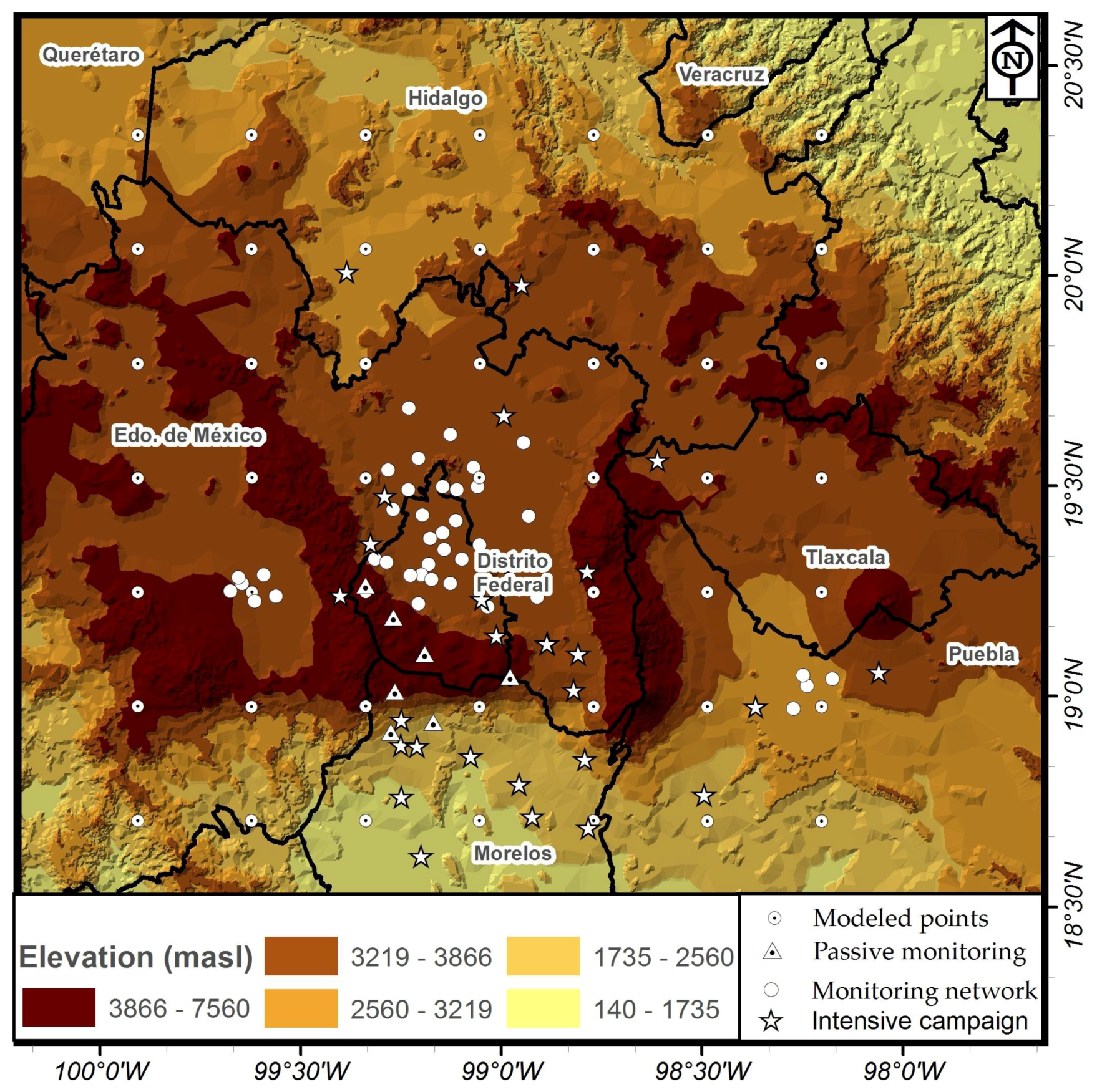
2.1. Study Area
2.2. Ozone Data
2.2.1. Passive Monitoring
2.2.2. Continuous Monitoring
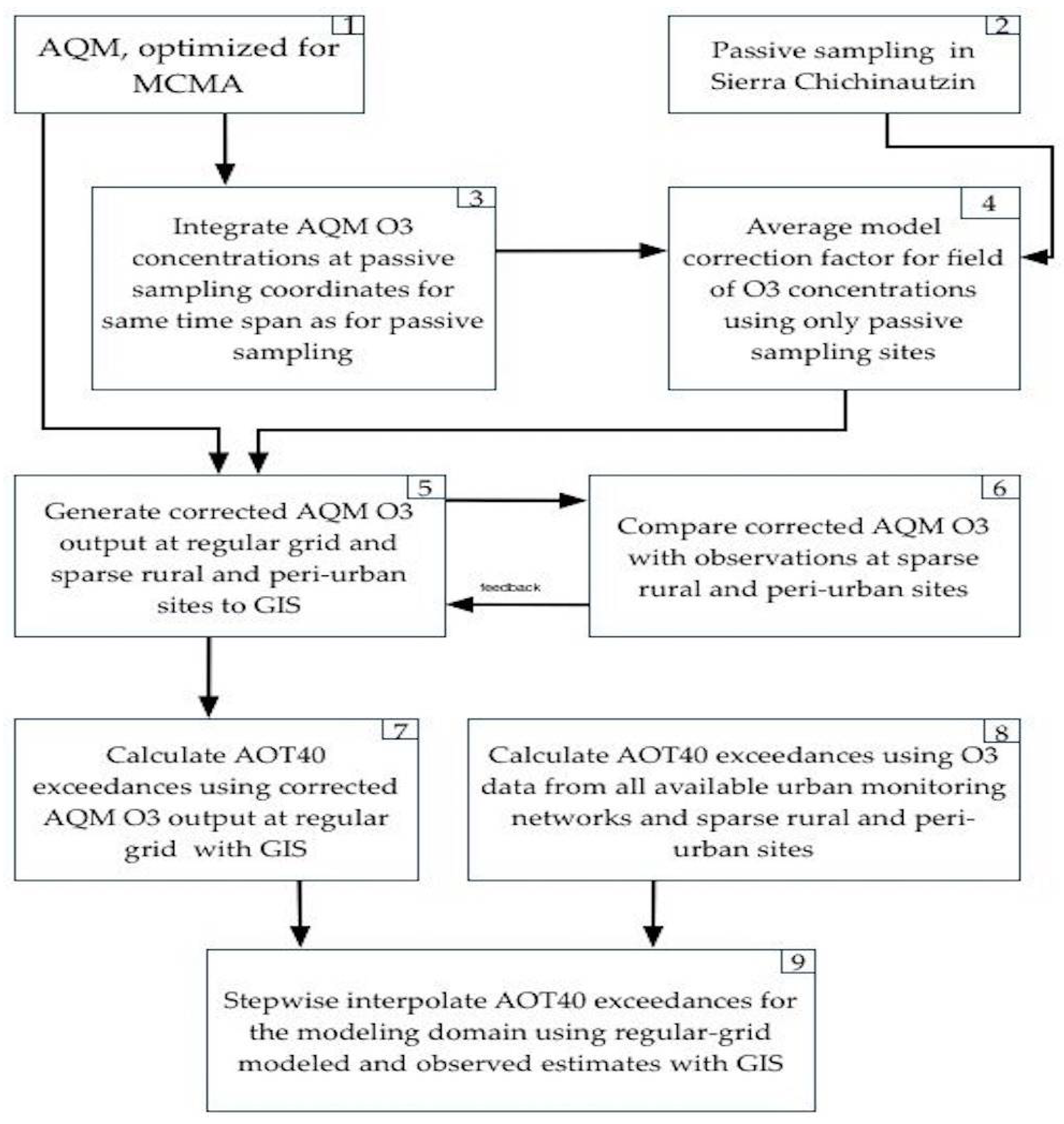
2.3. Maps
2.4. Exposure–Response Functions
2.5. Statistical Information
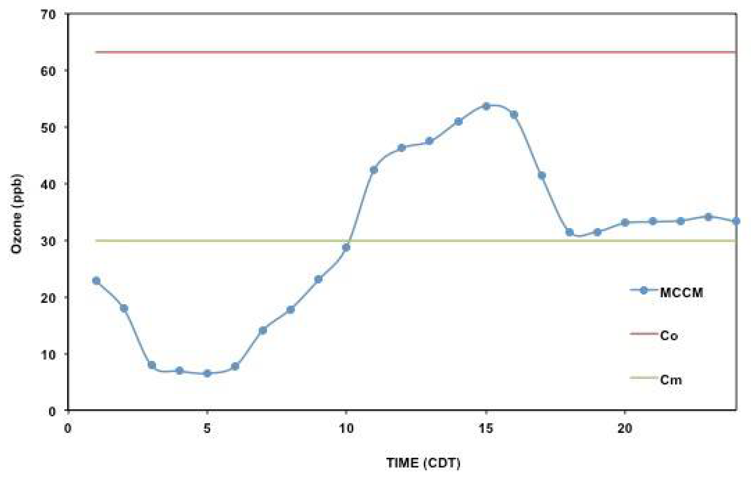
2.6. Air Quality Model
3. Results and Discussion
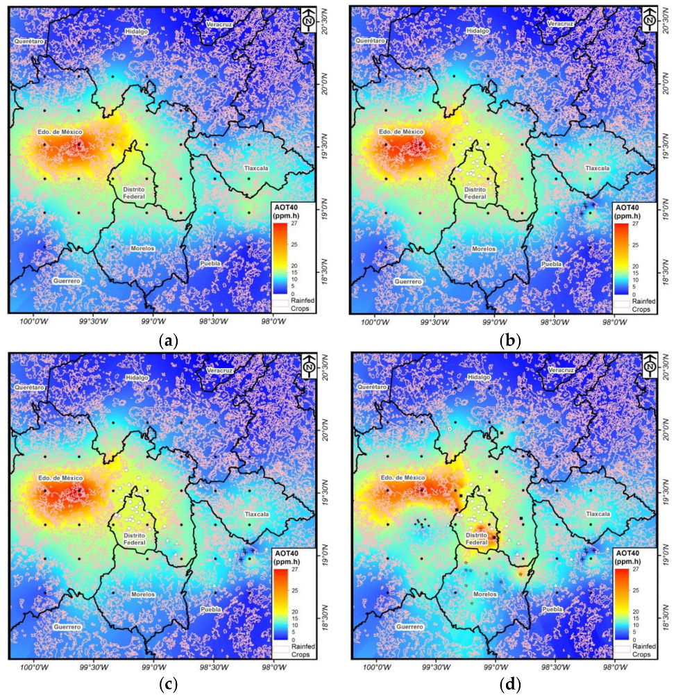
3.1. Creation of the Exceedance Maps
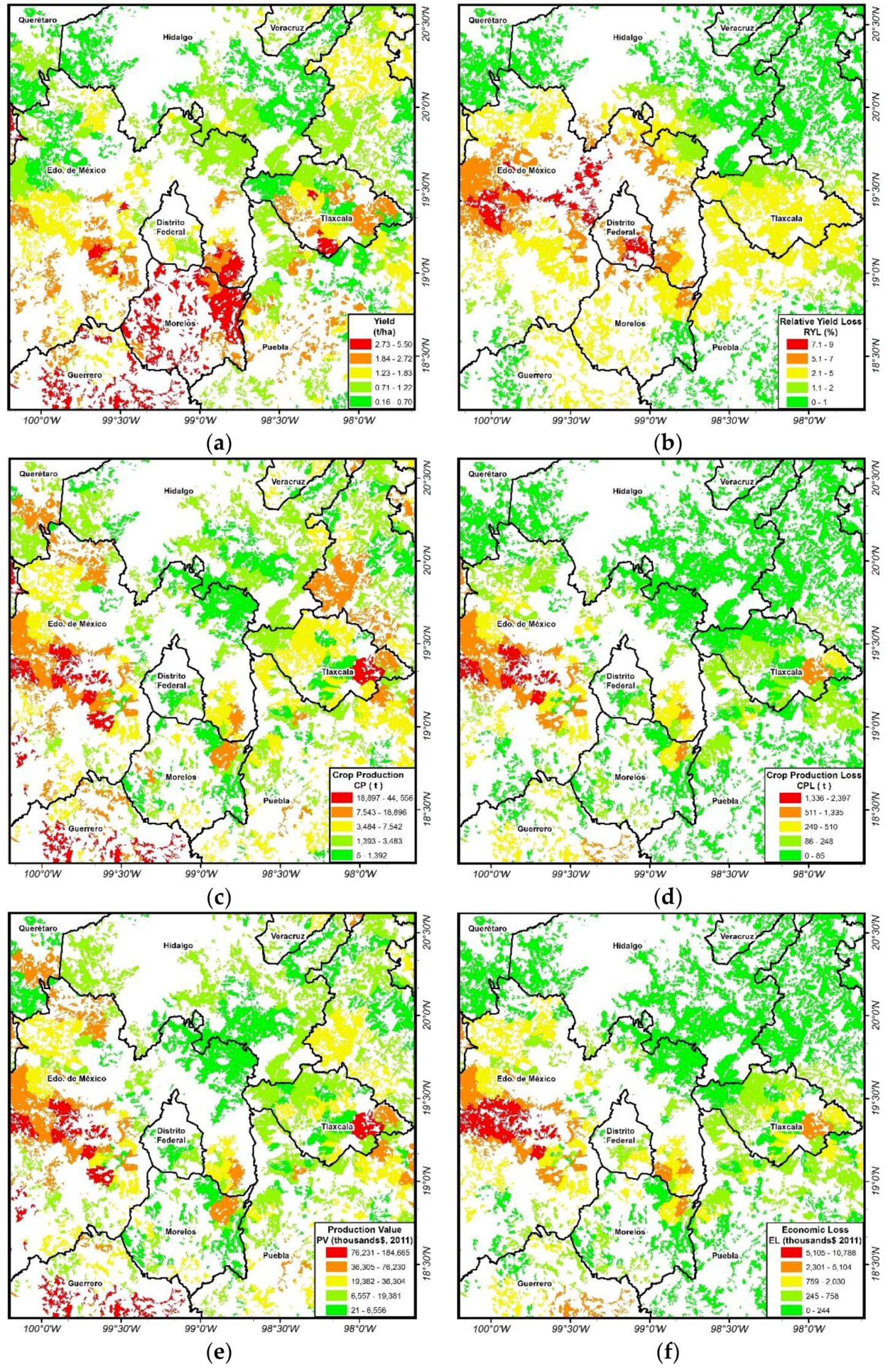
3.2. Estimation of Economic Losses
4. Conclusions
Author Contributions
Acknowledgments
Conflicts of Interest
References
- Thompson, A.M.; Yorks, J.E.; Miller, S.K.; Witte, J.C.; Dougherty, K.M.; Morris, G.A.; Baumgardner, D.; Ladino, L.; Rappenglück, B. Tropospheric ozone sources and wave activity over Mexico City and Houston during MILAGRO/Intercontinental Transport Experiment (INTEX-B) Ozonesonde Network Study, 2006 (IONS-06). Atmos. Chem. Phys. 2008, 8, 5113–5125. [Google Scholar] [CrossRef] [Green Version]
- Felzer, B.S.; Cronin, T.; Reilly, J.M.; Melillo, J.M.; Wang, X. Impacts of ozone on trees and crops. C. R. Geosci. 2007, 339, 784–798. [Google Scholar] [CrossRef] [Green Version]
- Logan, J.A. Tropospheric ozone: Seasonal behavior, trends, and anthropogenic influence. J. Geophys. Res. Atmos. 1985, 90, 10463–10482. [Google Scholar] [CrossRef]
- Gregg, J.W.; Jones, C.G.; Dawson, T.E. Urbanization effects on tree growth in the vicinity of New York City. Nature 2003, 424, 183–187. [Google Scholar] [CrossRef] [PubMed]
- Mauzerall, D.L.; Wang, X. Protecting agricultural crops from the effects of tropospheric ozone exposure: Reconciling science and standard setting in the United States, Europe, and Asia. Annu. Rev. Energy Environ. 2001, 26, 237–268. [Google Scholar] [CrossRef]
- Ganguly, N.D.; Tzanis, C. Study of stratosphere-troposphere exchange events of ozone in India and Greece using ozonesonde ascents. Meteorol. Appl. 2011, 18, 467–474. [Google Scholar] [CrossRef]
- De Bauer, M.D.; Hernandez-Tejeda, T. A review of ozone-induced effects on the forests of central Mexico. Environ. Pollut. 2007, 147, 446–453. [Google Scholar] [CrossRef] [PubMed]
- Hayes, F.; Mills, G.; Harmens, H.; Norris, D. Evidence of Widespread Ozone Damage to Vegetation in Europe (1990–2006); ICP Vegetation Programme Coordination Centre, CEH: Bangor, UK, 2007. [Google Scholar]
- Avnery, S.; Mauzerall, D.L.; Liu, J.; Horowitz, L.W. Global crop yield reductions due to surface ozone exposure: 1. Year 2000 crop production losses and economic damage. Atmos. Environ. 2011, 45, 2284–2296. [Google Scholar] [CrossRef]
- Fuhrer, J.; Skärby, L.; Ashmore, M.R. Critical levels for ozone effects on vegetation in Europe. Environ. Pollut. 1997, 97, 91–106. [Google Scholar] [CrossRef]
- Fuhrer, J. Critical level for ozone to protect agricultural crops: Interaction with water availability. Water Air Soil Pollut. 1995, 85, 1355–1360. [Google Scholar] [CrossRef]
- Mills, G.; Buse, A.; Gimeno, B.; Bermejo, V.; Holland, M.; Emberson, L.; Pleijel, H. A synthesis of AOT40-based response functions and critical levels of ozone for agricultural and horticultural crops. Atmos. Environ. 2007, 41, 2630–2643. [Google Scholar] [CrossRef]
- Musselman, R.C.; Lefohn, A.S.; Massman, W.J.; Heath, R.L. A critical review and analysis of the use of exposure- and flux-based ozone indices for predicting vegetation effects. Atmos. Environ. 2006, 40, 1869–1888. [Google Scholar] [CrossRef]
- Krupa, S.V.; Manning, W.J. Atmospheric ozone: Formation and effects on vegetation. Environ. Pollut. 1988, 50, 101–137. [Google Scholar] [CrossRef]
- Vlachokostas, C.; Nastis, S.A.; Achillas, C.; Kalogeropoulos, K.; Karmiris, I.; Moussiopoulos, N.; Chourdakis, E.; Banias, G.; Limperi, N. Economic damages of ozone air pollution to crops using combined air quality and GIS modelling. Atmos. Environ. 2010, 44, 3352–3361. [Google Scholar] [CrossRef]
- Van Dingenen, R.; Dentener, F.J.; Raes, F.; Krol, M.C.; Emberson, L.; Cofala, J. The global impact of ozone on agricultural crop yields under current and future air quality legislation. Atmos. Environ. 2009, 43, 604–618. [Google Scholar] [CrossRef]
- Chuwah, C.; van Noije, T.; van Vuuren, D.P.; Stehfest, E.; Hazeleger, W. Global impacts of surface ozone changes on crop yields and land use. Atmos. Environ. 2015, 106, 11–23. [Google Scholar] [CrossRef]
- Instituto Nacional de Ecología y Cambio Climático (INECC). Sistema Nacional de Indicadores de Calidad del Aire. Available online: http://sinaica.inecc.gob.mx/ (accessed on 9 March 2018).
- Semarnat. Programa de Gestión Federal para Mejorar la Calidad del Aire de la Megalópolis 2017–2030; Semarnat: Ciudad de México, México, 2017; p. 330. [Google Scholar]
- Goldan, P.D.; Trainer, M.; Kuster, W.C.; Parrish, D.D.; Carpenter, J.; Roberts, J.M.; Yee, J.E.; Fehsenfeld, F.C. Measurements of hydrocarbons, oxygenated hydrocarbons, carbon monoxide, and nitrogen oxides in an urban basin in Colorado: Implications for emission inventories. J. Geophys. Res.-Atmos. 1995, 100, 22771–22783. [Google Scholar] [CrossRef]
- Coyle, M.; Smith, R.I.; Stedman, J.R.; Weston, K.J.; Fowler, D. Quantifying the spatial distribution of surface ozone concentration in the UK. Atmos. Environ. 2002, 36, 1013–1024. [Google Scholar] [CrossRef]
- Krupa, S.V.; Legge, A.H. Passive sampling of ambient, gaseous air pollutants: An assessment from an ecological perspective. Environ. Pollut. 2000, 107, 31–45. [Google Scholar] [CrossRef]
- Carmichael, G.R.; Ferm, M.; Thongboonchoo, N.; Woo, J.-H.; Chan, L.Y.; Murano, K.; Viet, P.H.; Mossberg, C.; Bala, R.; Boonjawat, J. Measurements of sulfur dioxide, ozone and ammonia concentrations in Asia, Africa, and south America using passive samplers. Atmos. Environ. 2003, 37, 1293–1308. [Google Scholar] [CrossRef]
- Cox, R.M.; Malcolm, J.W. Passive ozone monitoring for forest health assessment. Water Air Soil Pollut. 1999, 116, 339–344. [Google Scholar] [CrossRef]
- Krupa, S.; Nosal, M.; Peterson, D.L. Use of passive ambient ozone (O3) samplers in vegetation effects assessment. Environ. Pollut. 2001, 112, 303–309. [Google Scholar] [CrossRef]
- Gerosa, G.; Ferretti, M.; Bussotti, F.; Rocchini, D. Estimates of ozone aot40 from passive sampling in forest sites in south-western Europe. Environ. Pollut. 2007, 145, 629–635. [Google Scholar] [CrossRef] [PubMed]
- Loibi, W.; Winiwarter, W.; Kopsca, A.; Zufger, J.; Baumann, R. Estimating the spatial distribution of ozone concentrations in complex terrain. Atmos. Environ. 1994, 28, 2557–2566. [Google Scholar] [CrossRef]
- Simpson, D. Photochemical model calculations over Europe for two extended summer periods: 1985 and 1989. Model results and comparison with observations. Atmos. Environ. Part A Gen. Top. 1993, 27, 921–943. [Google Scholar] [CrossRef]
- Tarrasón, L.; Semb, A.; Hjellbrekke, A.G.; Tsyro, S.; Schaug, J.; Bartnicki, J.; Solberg, S. Geographical Distribution of Sulphur and Nitrogen Compounds in Europe Derived both from Modelled and Observed Concentrations; 71; Norwegian Meteorological Institute: Kjeller, Norway, 1998. [Google Scholar]
- Bush, T.; Targa, J.; Stedman, J. UK Air Quality Modelling for Annual Reporting 2004 on Ambient Air Quality Assessment under Council Directives 96/62/EC and 2002/3/EC Relating to Ozone in Ambient Air; Department for Environment, Food and Rural Affairs, Welsh Assembly Government, the Scottish Executive and the Department of the Environment for Northern Ireland: Didcot, UK, 2007.
- Denby, B.; Horálek, O.J.; Walker, S.E.; Eben, K.; Fiala, J. Interpolation and Assimilation Methods for European Scale Air Quality Assessment and Mapping Part I: Review and Recommendations; European Topic Centre on Air and Climate Change: Bilthoven, The Netherlands, 2005; p. 51. [Google Scholar]
- De Bauer, L.I.; Krupa, S.V. The valley of Mexico: Summary of observational studies on its air quality and effects on vegetation. Environ. Pollut. 1990, 65, 109–118. [Google Scholar] [CrossRef]
- Ortíz-García, C.F.; Laguette-Rey, H.D.; de Bauer, L.I. Effects of oxidants in ambient air on annual crops in the basin of Mexico. In Urban Air Pollution and Forests. Ecological Studies (Analysis and Synthesis); Fenn, M.E., de Bauer, L.I., Hernández-Tejeda, T., Eds.; Springer: New York, NY, USA, 2002; Volume 156, pp. 320–333. [Google Scholar]
- Instituto Nacional de Estadística y Geografía (INEGI). Censo de Población y Vivienda 2010. Principales Resultados por Área Geoestadística Básica (AGEB); Instituto Nacional de Estadística y Geografía: Aguascalientes, México, 2011. [Google Scholar]
- Instituto Nacional de Estadística y Geografía (INEGI). Conjunto de Datos Vectoriales de Uso de Suelo y Vegetación Escala 1:250,000; Serie IV (2007–2010); Instituto Nacional de Estadística y Geografía: Aguascalientes, México, 2010. [Google Scholar]
- Instituto Nacional de Estadística y Geografía (INEGI). Banco de Información Económica (BIE); Instituto Nacional de Estadística y Geografía: Aguascalientes, México, 2011. [Google Scholar]
- Koutrakis, P.; Wolfson, J.M.; Bunyaviroch, A.; Froehlich, S.E.; Hirano, K.; Mulik, J.D. Measurement of ambient ozone using a nitrite-coated filter. Anal. Chem. 1993, 65, 209–214. [Google Scholar] [CrossRef]
- Sedema. Estaciones de Monitoreo. Available online: http://www.aire.df.gob.mx/default.php?opc=‘ZaBhnmI=&dc=‘ZA== (accessed on 8 March 2018).
- Salcedo, D.; Castro, T.; Ruiz-Suárez, L.G.; García-Reynoso, A.; Torres-Jardón, R.; Torres-Jaramillo, A.; Mar-Morales, B.E.; Salcido, A.; Celada, A.T.; Carreón-Sierra, S.; et al. Study of the regional air quality south of Mexico City (Morelos state). Sci. Total Environ. 2012, 414, 417–432. [Google Scholar] [CrossRef] [PubMed]
- García-Yee, J.S.; Torres-Jardón, R.; Barrera-Huertas, H.; Castro, T.; Peralta, O.; García, M.; Gutiérrez, W.; Robles, M.; Torres-Jaramillo, A.; Ortínez, A.; et al. Characterization of NOx-Ox relationships during daytime interchange of air masses over a mountain pass in the Mexico City megalopolis. Atmos. Environ. 2018, 177, 100–110. [Google Scholar] [CrossRef]
- Barrera-Huertas, H.; Torres, R.; Ruiz-Suárez, L.; Garcia, J.; Gutierrez, W.; Torres, A. Analysis of ozone transportation in Tlaxcala-Puebla Mexico air basin. In AGU Fall Meeting Abstracts; American Geophysical Union: Washington, DC, USA, 2014; p. 3213. [Google Scholar]
- Instituto Nacional de Estadística y Geografía (INEGI). Marco Geoestadístico Nacional (MGN) V.5.0.; Instituto Nacional de Estadística y Geografía: Aguascalientes, México, 2010. [Google Scholar]
- Hengl, T. A Practical Guide to Geostatistical Mapping of Environmental Variables; JRC Scientific and Technical Reports; Publications Office of the European Union: Luxembourg, 2007; p. 270. [Google Scholar]
- Li, J.; Heap, A.D. A Review of Spatial Interpolation Methods for Environmental Scientists; Geoscience Australia: Canberra, Australia, 2008; p. 137.
- Oficina Estatal de Información para el Desarrollo Rural Sustentable (OEIDRUS). Sistema de Información Geográfica de Morelos; Oficina Estatal de Información para el Desarrollo Rural Sustentable: Cuernavaca, Mexico, 2014. [Google Scholar]
- Secretaría de Agricultura, Ganadería, Desarrollo Rural, Pesca y Alimentación (SAGARPA). Servicio de Información Agroalimentaria y Pesquera (SIAP); Secretaría de Agricultura, Ganadería, Desarrollo Rural, Pesca y Alimentación: Ciudad de México, México, 2011. [Google Scholar]
- Consejo Nacional de Población (CONAPO). Índice de Marginación por Localidad; Consejo Nacional de Población: Ciudad de México, México, 2012. [Google Scholar]
- Grell, G.A.; Emeis, S.; Stockwell, W.R.; Schoenemeyer, T.; Forkel, R.; Michalakes, J.; Knoche, R.; Seidl, W. Application of a multiscale, coupled MM5/chemistry model to the complex terrain of the VOTALP valley campaign. Atmos. Environ. 2000, 34, 1435–1453. [Google Scholar] [CrossRef]
- Stockwell, W.R.; Middleton, P.; Chang, J.S.; Tang, X. The second generation regional acid deposition model chemical mechanism for regional air quality modeling. J. Geophys. Res. Atmos. 1990, 95, 16343–16367. [Google Scholar] [CrossRef]
- Willmott, C.J. On the validation of models. Phys. Geogr. 1981, 2, 184–194. [Google Scholar]
- Song, J.; Lei, W.; Bei, N.; Zavala, M.; De Foy, B.; Volkamer, R.; Cardenas, B.; Zheng, J.; Zhang, R.; Molina, L.T. Ozone response to emission changes: A modeling study during the MCMA-2006/MILAGRO Campaign. Atmos. Chem. Phys. 2010, 10, 3827–3846. [Google Scholar] [CrossRef] [Green Version]
- Lei, W.; de Foy, B.; Zavala, M.; Volkamer, R.; Molina, L.T. Characterizing ozone production in the Mexico City metropolitan area: A case study using a chemical transport model. Atmos. Chem. Phys. 2007, 7, 1347–1366. [Google Scholar] [CrossRef]
- Jazcilevich, A.; Garcia, A.; Ruiz-Suarez, L. A modeling study of air pollution modulation through land-use change in the valley of Mexico. Atmos. Environ. 2002, 36, 2297–2307. [Google Scholar] [CrossRef]
- Escalante García, J.S.; García Reynoso, J.A.; Jazcilevich Diamant, A.; Ruiz-Suárez, L.G. The influence of the Tula, Hidalgo complex on the air quality of the Mexico City Metropolitan Area. Atmósfera 2014, 27, 215–225. [Google Scholar] [CrossRef] [Green Version]
- Ruiz Suárez, L.; Longoria, R.; Hernandez, F.; Segura, E.; Trujillo, A.; Conde, C. Emisiones biogénicas de hidrocarburos no-metano y de oxido nítrico en la cuenca del valle de México. Atmosfera 1999, 12, 89–100. [Google Scholar]
- Barrera-Huertas, T.-J.R.; Ruíz-Suárez, L.G.; García-Yee, J.S.; Torres-Jaramillo, A.; Martínez, A.P.; Gutierrez, W.; García, L.M.; Robles, M.; Retama, A.; García-Reynoso, J.A. Análisis del transporte de ozono en la cuenca atmosférica de puebla-tlaxcala en el centro de México. Atmosfera 2017. submitted. [Google Scholar]
- Mendoza Flores, A. Análisis de la Calidad del Aire Alrededor del Complejo Industrial en Tula Durante el 2008; Universidad Nacional Autónoma de México (UNAM): Ciudad de México, México, 2011. [Google Scholar]
- Granada-Macias, L.M.; Rosas-Perez, R.; Torres-Jardon, R. Ozone levels at a high altitude suburban abies religiosa forest on the western slope of a mountain range under the influence of the Mexico City and Toluca Valley urban areas. Environ. Monit. Assess. 2018. submited. [Google Scholar]
- Molina, L.T.; Madronich, S.; Gaffney, J.S.; Apel, E.; de Foy, B.; Fast, J.; Ferrare, R.; Herndon, S.; Jimenez, J.L.; Lamb, B.; et al. An overview of the milagro 2006 campaign: Mexico city emissions and their transport and transformation. Atmos. Chem. Phys. 2010, 10, 8697–8760. [Google Scholar] [CrossRef] [Green Version]
- Garcia-Reynoso, A.; Jazcilevich, A.; Ruiz-Suarez, L.G.; Torres-Jardon, R.; Lastra, M.S.; Juarez, N.A.R. Ozone weekend effect analysis in Mexico City. Atmosfera 2009, 22, 281–297. [Google Scholar]
- Instituto Nacional de Ecología y Cambio Climático (INECC). Estudios de Calidad del Aire y su Impacto en la Región Centro de México (ECAIM); Instituto Nacional de Ecología y Cambio Climático: Ciudad de México, México, 2014; p. 744. [Google Scholar]
- Instituto Nacional de Ecología y Cambio Climático (INECC). Evaluación de las Capacidades Técnicas y de Infraestructura de los Laboratorios Institucionales; Instituto Nacional de Ecología y Cambio Climático: Ciudad de México, Mexico, 2015; p. 25. [Google Scholar]
- De Foy, B.; Krotkov, N.A.; Bei, N.; Herndon, S.C.; Huey, L.G.; Martínez, A.-P.; Ruiz-Suárez, L.G.; Word, E.C.; Zavala, M.; Molina, L.T. Hit from both sides: Tracking industrial and volcanic plumes in Mexico City with surface measurements and OMI SO2 retrievals during the MILAGRO field campaign. Atmos. Chem. Phys. 2009, 9, 9599–9617. [Google Scholar] [CrossRef]


| Crop | ERFs Used for RYL Calculation, AOT40 [ppm·h] | Critical Level * [ppm·h] |
|---|---|---|
| Maize | −0.0035 * AOT40 | 13.9 |
| Sensitive crops (oats, sorghum, and beans) | −0.01212 * AOT40 | 3 |
| Tres Marías | CICS | Desierto de los Leones | Lomas de Ahuatlan | Parres | Santa Catarina | San Nicolas | |
|---|---|---|---|---|---|---|---|
| Cold dry 2009 | 3.21 | 1.63 | 1.14 | 1.48 | 2.29 | 3.02 | 1.68 |
| Cold dry 2010 | 4.20 | 1.64 | 1.13 | 1.50 | 2.05 | 4.37 | 1.52 |
| Cold dry 2011 | 3.40 | 1.58 | 1.09 | 1.45 | 2.21 | 3.16 | 1.62 |
| Cold dry average | 3.60 | 1.62 | 1.12 | 1.48 | 2.18 | 3.52 | 1.61 |
| Warm dry 2009 | 3.24 | 1.37 | 0.76 | 1.53 | 2.02 | 3.26 | 1.29 |
| Warm dry 2010 | 3.50 | 1.37 | 0.79 | 1.54 | 1.95 | 3.68 | 1.30 |
| Warm dry 2011 | 3.39 | 1.37 | 0.76 | 1.51 | 1.92 | 3.58 | 1.25 |
| Warm dry average | 3.37 | 1.37 | 0.77 | 1.52 | 1.96 | 3.51 | 1.28 |
| Dry season average | 3.49 | 1.49 | 0.94 | 1.50 | 2.07 | 3.51 | 1.44 |
| Std dev cold + warm dry | 0.36 | 0.14 | 0.19 | 0.03 | 0.15 | 0.49 | 0.19 |
| State | Municipality | AOT40 (ppm·h) | Relative Yield Loss (%) | Yield (t/ha) | Yield Loss (t/ha) | Economic Loss/ha (MXN/ha) | Sown Area (ha) | Production Value (Millions of Pesos MXN) | Economic Loss (Millions of Pesos MXN) | Degree of Marginalization |
|---|---|---|---|---|---|---|---|---|---|---|
| Mexico | Villa de Allende | 23.98 | 7 | 2.50 | 0.18 | 799 | 13,500 | 152 | 11 | High |
| Mexico | Toluca | 18.28 | 5 | 2.50 | 0.12 | 497 | 17,822 | 185 | 9 | Very low |
| Mexico | Almoloya de Juarez | 24.95 | 7 | 1.34 | 0.10 | 382 | 21,000 | 107 | 8 | Medium |
| Mexico | Villa Victoria | 25.84 | 7 | 1.40 | 0.11 | 496 | 12,100 | 76 | 6 | High |
| Tlaxcala | Huamantla | 14.33 | 3 | 2.40 | 0.08 | 352 | 14,480 | 156 | 5 | Low |
| Mexico | Tenango del Valle | 18.05 | 4 | 2.60 | 0.12 | 520 | 8891 | 98 | 5 | Low |
| Mexico | Ixtlahuaca | 27.40 | 8 | 0.80 | 0.07 | 313 | 12,903 | 47 | 4 | Medium |
| Mexico | Lerma | 21.83 | 6 | 1.50 | 0.09 | 355 | 9989 | 57 | 4 | Very low |
| Mexico | San Jose del Rincón | 23.25 | 6 | 0.85 | 0.06 | 246 | 13,173 | 48 | 3 | High |
| Mexico | Amecameca | 18.31 | 5 | 3.27 | 0.16 | 699 | 4553 | 66 | 3 | Low |
| Mexico | Temoaya | 26.28 | 7 | 1.94 | 0.16 | 556 | 5600 | 39 | 3 | Medium |
| Mexico | Zinacantepec | 18.95 | 5 | 1.66 | 0.08 | 320 | 9557 | 60 | 3 | Low |
| Mexico | Tianguistenco | 19.76 | 5 | 2.50 | 0.13 | 579 | 5251 | 56 | 3 | Low |
| Mexico | Amanalco | 22.16 | 6 | 1.60 | 0.10 | 458 | 6500 | 47 | 3 | Medium |
| Guerrero | Huitzuco | 13.84 | 3 | 3.00 | 0.09 | 322 | 8971 | 94 | 3 | High |
| Mexico | Donato Guerra | 22.81 | 6 | 1.32 | 0.09 | 394 | 7200 | 43 | 3 | High |
| Michoacan | Zitacuaro | 23.74 | 7 | 1.75 | 0.12 | 359 | 7550 | 39 | 3 | Medium |
| Morelos | Ocuituco | 23.60 | 6 | 3.18 | 0.22 | 838 | 3010 | 36 | 3 | Medium |
| Guerrero | Iguala | 11.32 | 2 | 5.50 | 0.12 | 560 | 4337 | 114 | 2 | Low |
| Michoacan | Contepec | 14.55 | 3 | 3.00 | 0.10 | 271 | 8545 | 69 | 2 | Medium |
| Total | 194,932 | 1590 | 85 |
| Crop | Sown Area (ha) | Production Value (In Millions of Pesos MXN) | Economic Loss (In Millions of Pesos MXN) |
|---|---|---|---|
| Maize | 1,132,150 | 6598 | 191 |
| Oats (grain) | 26,087 | 98 | 25 |
| Oats (forage) | 153,154 | 1133 | 310 |
| Beans | 61,128 | 357 | 51 |
| Sorghum | 53,524 | 620 | 94 |
© 2018 by the authors. Licensee MDPI, Basel, Switzerland. This article is an open access article distributed under the terms and conditions of the Creative Commons Attribution (CC BY) license (http://creativecommons.org/licenses/by/4.0/).
Share and Cite
Ruiz-Suárez, L.G.; Mar-Morales, B.E.; García-Reynoso, J.A.; Andraca-Ayala, G.L.; Torres-Jardón, R.; García-Yee, J.S.; Barrera-Huertas, H.A.; Gavilán-García, A.; Basaldud Cruz, R. Estimation of the Impact of Ozone on Four Economically Important Crops in the City Belt of Central Mexico. Atmosphere 2018, 9, 223. https://doi.org/10.3390/atmos9060223
Ruiz-Suárez LG, Mar-Morales BE, García-Reynoso JA, Andraca-Ayala GL, Torres-Jardón R, García-Yee JS, Barrera-Huertas HA, Gavilán-García A, Basaldud Cruz R. Estimation of the Impact of Ozone on Four Economically Important Crops in the City Belt of Central Mexico. Atmosphere. 2018; 9(6):223. https://doi.org/10.3390/atmos9060223
Chicago/Turabian StyleRuiz-Suárez, Luis Gerardo, Bertha Eugenia Mar-Morales, José Agustín García-Reynoso, Gema Luz Andraca-Ayala, Ricardo Torres-Jardón, José Santos García-Yee, Hugo Alberto Barrera-Huertas, Arturo Gavilán-García, and Roberto Basaldud Cruz. 2018. "Estimation of the Impact of Ozone on Four Economically Important Crops in the City Belt of Central Mexico" Atmosphere 9, no. 6: 223. https://doi.org/10.3390/atmos9060223