Application of Intelligent Dynamic Bayesian Network with Wavelet Analysis for Probabilistic Prediction of Storm Track Intensity Index

Abstract

The effective prediction of storm track (ST) is greatly beneficial for analyzing the development and anomalies of mid-latitude weather systems. For the non-stationarity, nonlinearity, and uncertainty of ST intensity index (STII), a new probabilistic prediction model was proposed based on dynamic Bayesian network (DBN) and wavelet analysis (WA). We introduced probability theory and graph theory for the first time to quantitatively describe the nonlinear relationship and uncertain interaction of the ST system. Then a casual prediction network (i.e., DBN) was constructed through wavelet decomposition, structural learning, parameter learning, and probabilistic inference, which was used for expression of relation among predictors and probabilistic prediction of STII. The intensity prediction of the North Pacific ST with data from 1961–2010 showed that the new model was able to give more comprehensive prediction information and higher prediction accuracy and had strong generalization ability and good stability.

1. Introduction

One of the primary features of mid- and high-latitude atmospheric circulation (AC) is transient variability, which is closely related to the growth and decay of daily weather systems. In the 1970s, Blackmon [1] found sub-weekly (2.5–6 days) transient eddies over the North Pacific and North Atlantic with filtering data. He defined the two zonal-extended regions with the most intensive transient variability as “storm track” (ST), which can be divided, respectively, into North Pacific ST (NPST) and North Atlantic ST (NAST). ST corresponds significantly with cyclone and anticyclone activities, which can be the indication of the development of weather systems. Moreover, as a contacting link of heat and kinetic energy between ocean and atmosphere, ST plays an important role in the maintenance of AC and climate change [2].

ST is crucial to the short-term anomaly of AC with interactions between ST and low-frequency circulation. So far, many studies have revealed the interaction. Lau [3] studied the seasonal variation of ST and pointed out that the main mode of the variation was related to the teleconnection pattern of the low-frequency circulation in the northern hemisphere. Straus et al. [4] discovered that the ST anomaly was closely related to the sea surface temperature (SST) anomaly in the Kuroshio area. Zhu et al. [5] summarized the correlation between the winter NPST and the Pacific-North America teleconnection pattern (PNA) and Western Pacific teleconnection pattern (WP). Ren et al. [6] used the empirical orthogonal function (EOF) to analyze the temporal and spatial variability of the winter NPST and explained its coupled pattern with the mid-latitude air-sea system. Liu et al. [7] determined the correlation and potential influencing mechanisms between the Polar vortex intensity and NPST. Both observational research and theoretical studies have indicated the symbiotic relationship between ST and large-scale AC in the Northern Hemisphere. However, most studies are just diagnostic analysis about ST variability and correlation. To grasp the evolvement role of ST, prediction is becoming an urgent area of research.

However, ST is a highly nonlinear system due to nonlinear processes in the air-sea system. There is relatively little research on the numerical forecasting or statistical forecasting of ST both at home and abroad. That may result from the diversity of influencing factors and the complexity of correlation mechanisms. In addition, strong transients and uncertain rules have also caused difficulties in ST prediction. In meteorological prediction, climate indexes are often used as predictands and predictors to explain the behavior of future climate. Therefore, how to quantify the intensity and spatial-temporal variation as indexes is the premise of ST prediction. At present, there are several indexes that can indicate the possible evolution of ST, whose calculation methods with filtering variance includes the central point representation [8,9], regional average [10], and EOF [11]. The above studies achieve the quantitative description of the nonlinear ST system by establishing an index. Thus, we can predict the temporal and spatial variation of ST with the ST index.

The prediction of ST index belongs to the prediction of nonlinear time-series. In the field of meteorology and oceanology, data-driven models (i.e., statistical models) are suitable predicting tools due to their rapid development times, as well as low information requirements compared to physical-based models. Hong et al. [12] introduced the inversion idea and used genetic algorithm to reconstruct the nonlinear forecasting model of the subtropical high index from historical data. Liu et al. [13] integrated the EOF, wavelet decomposition and support vector machine (SVM) method to predict the 500 $\mathrm{hPa}$ geopotential height in summer. Zhu et al. [14] conducted a short-term forecast experiment of the tropical atmospheric seasonal oscillation (MJO) index, using both the singular spectrum analysis and auto-regression model. Jia et al. [15] applied the correlation analysis and optimal subset regression to select predictors and established a statistical prediction model for the subtropical high index. The above statistical methods require a large amount of historical data, but their efficiency on processing big data is low. Most importantly, these methods have weak ability to mine and express the internal relations from data quantitatively. Therefore, the above models are still flawed for prediction of ST index.

With the rapid development of computer technology and information acquisition technology, machine learning (ML) and data mining (DM) have opened a new era—artificial intelligence. Breakthroughs have been made by the application of ML and DM in the fields of biology, finance, and medicine [16,17,18], and they have also brought opportunities for the development of predicting technology in meteorology and oceanology. Many scholars have applied ML and DM to meteorological prediction: Yang et al. [19] used the association rules mining to analyze the data set of North Atlantic hurricane history trace and predicted the intensity of the North Atlantic hurricane based on the mining results. Royston et al. [20] applied the semantic decision tree to conduct regular mining and forecast modeling with water level and meteorological data, to forecast the storm surge of Thames Estuary. Gordon et al. [21] constructed a meteorological prediction model using neural network (NN) and frequency domain algorithm to implement 24-hour refined prediction. Teng [22] extracted highly relevant factors and used the stepwise regression and SVM to establish the medium-term prediction model of the tropical cyclone path in the Western Pacific.

To a certain extent, ML and DM can overcome the shortcomings of the above statistical methods and achieve data mining and reasoning with rapid development times. However, the above ML algorithms are all deterministic methods, that is, give a certain value for a certain predicting moment. Please note that ST is affected by the nonlinear action of various weather systems and has strong uncertainties. When the intensity and position of ST fluctuate greatly, deterministic single-point prediction may not achieve the desired accuracy. In contrast, the probabilistic prediction method could give the result in the form of probability distribution, covering more complete prediction information.

As a new branch of ML theory, Bayesian network (BN) makes it feasible for the probabilistic prediction of ST index, which has been initially used in the field of meteorology and hydrology [23,24]. The emerging dynamic Bayesian Network (DBN) adds time information to the classical BN, which becomes a new probabilistic expression and reasoning tool owing to the ability to deal with uncertainties. Correspondingly, ST is affected by many factors in the mid-latitude air-sea system. There are random and non-linear interactions between these factors at same and different time. The features coincide exactly with the DBN, thus DBN is a powerful theoretical tool for probabilistic prediction of ST index. Additionally, note that time-series of the ST index is non-stationary. This limitation with non-stationary data has led to the recent formation of hybrid models, where data is preprocessed for non-stationary characteristics and then run through a predicting method such as ML algorithms to cope with the nonlinearity. Wavelet analysis (WA), an effective tool to deal with non-stationary data, has recently been applied to meteorological forecast. We will combine WA with DBN to achieve scientific and accurate prediction of ST index.

In this paper, we constructed the WA-DBN model to predict the winter PST intensity index. To deal with the non-stationarity, nonlinearity, and uncertainty, we introduced DBN theory innovatively and combined WA to establish a data-driven model for predicting the monthly STII using large-scale climate indexes as the predictors. We first selected the climate indexes significantly related to ST as predictors. Then based on wavelet decomposition, a WA-DBN probabilistic prediction model was constructed through structure learning, parameter learning and probabilistic reasoning. Finally, a deeper comparative analysis of model performance is conducted with key statistical indicators.

2. Theory and Method

2.1. Definition of Storm Track Intensity Index

To quantitatively describe the intensity of ST and its spatial-temporal variation, we refer to the existing definition method to calculate the intensity index. We identify the ST as the sub-weekly transient of the 500 $\mathrm{hPa}$ geopotential height. First sub-weekly transient eddies are derived from the geopotential height based on 31 symmetrical digital filter [25]. Then we calculate the monthly average band-pass filtering variance, selecting all grid points with the filtering variance greater than a certain fixed threshold, of which the mean value is defined as the ST intensity index (STII). The fixed threshold is usually taken as 20 ${\mathrm{dagpm}}^2$.

2.2. Dynamic Bayesian Network Theory

Bayesian Network (BN) was proposed by Judea Pearl in 1988, including the static Bayesian Network (SBN) and the dynamic Bayesian Network (DBN). Based on probability theory and graph theory, DBN integrates the time dimension into SBN to represent the temporal correlation, which forms a dynamic reasoning model with dynamic analysis and prediction of temporal information [26].

According to Bayesian theory, BN is a directed acyclic graph expressing the probabilistic relation between variables. It is mainly composed of nodes, directed arcs, and conditional probability distribution (CPT). DBN is an extension of SBN in the time dimension, and can be explained by a bigram $<B_0,B_{\to }>$:

• $B_0$ denotes the initial network, that is the SBN of each time slice. It contains the network structure and probability distribution of nodes at the same time;
• $B_{\to }$ denotes the transition network. It contains the causal link and the transition probability distribution of nodes in different time slice.

Define a variable set $X=\left[X_1,X_2,\cdots ,X_n\right]$ and a finite time segment $\left[0,1,\cdots ,T\right]$, then the joint probability distribution of $X^0,\dots ,X^T$ is

$$P(X^0,\dots ,X^T)=P(X^0)\cdot {\displaystyle \prod }_{t=1}^T{\displaystyle \prod }_{i=1}^{N}P\left[X_i^t|\pi \left(X_i^t\right)\right].$$

(1)

where $X_i^t$ denotes the node $i$ located in $t$ time slice, $\pi \left(X_i^t\right)$ denotes the parent of $X_i^t$. Formula (1) denotes the probabilistic reasoning of different time slices and different node states.

The construction of DBN includes structure learning and parameter learning: the former needs to construct $B_0$ and $B_{\to }$; the latter needs to determine the initial probability $P(X^0)$, the observation conditional probability $P\left[X_i^t|\pi \left(X_i^t\right)\right]$, and the transition conditional probability $P(X^t|X^{t-1})$. There are two common learning technologies for DBN: manual construction based on expert knowledge and automatic learning based on intelligent algorithms [27]. We adopt a combination of subjective and objective methods for DBN learning. Expert knowledge is used for structural learning while objective data is used for parameter learning.

2.3. Wavelet Analysis

Wavelet analysis (WA) is a mathematical function that can be used for the analysis of time-series that contain non-stationarities [28]. WA of the input variables can analyze various similarities within the dataset by decomposing data into different levels. Large-scale frequencies are checked with approximation series, while small-scale frequencies are checked by details (4–5 levels of decomposition). Wavelet decomposition gives time frequency representation of a signal at different temporal domains, providing considerable information about the physical structure of the data. Wavelet reconstruction can synthesize the different frequency signals to achieve information integration. The application of WA in meteorology and oceanology is relatively mature [29,30], therefore this paper will not give unnecessary details.

3. Probabilistic Prediction Model Based on WA and DBN

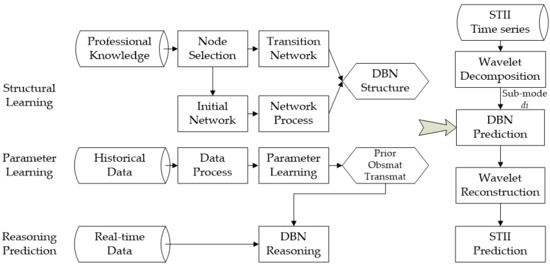
The STII prediction model based on WA and DBN (WA-DBN) was proposed for two problems: First, the time-series of intensity index is nonlinear due to strong transient; second, both ST intensity and predictors contain probabilistic uncertainties. Figure 1 displays the technical structure of WA-DBN model.

Seen from Figure 1, the WA-DBN prediction model includes two modules: WA module and DBN prediction module. WA is used for the decomposition and reconstruction of non-stationary time series. DBN is used for probabilistic prediction through structure learning, parameter learning and inference calculation, which is the core of this prediction model.

3.1. Structural Learning

The DBN structure describing the casual relation between various weather systems and the STII is the basis of intensity index prediction. The structural learning includes the selection of node variables and the determination of the dependencies among nodes. We adopt an expert-constructed method for structural learning. Based on professional knowledge, the predictors are selected as child nodes of the DBN and a causal topology is constructed, including the initial network and the transition network.

3.1.1. Node Determination—Predictor Selection

We choose key factors that have significant influence on the ST as network nodes. Winter ST relates to many members in the North Pacific atmosphere-ocean system. Limpasuvan et al. [31] pointed out that the weakening of the stratospheric polar vortex would affect the changes of the ST and jet; Gao [32] conducted a preliminary exploration of the relationship between winter NPST and Arctic Oscillation (AO) index, and discovered that AO and NPST had the same phase of strong and weak variation; Gu et al. [33] determined the relationship between NPST anomaly in winter and the AC in East Asia. In addition, the NPST intensity is closely related to the atmospheric system, such as the WP and PNA teleconnection patterns, jet flow anomaly, monsoon activity, the Aleutian low pressure, Siberian high, and the ocean circulation and SST anomaly [34,35,36,37,38,39].

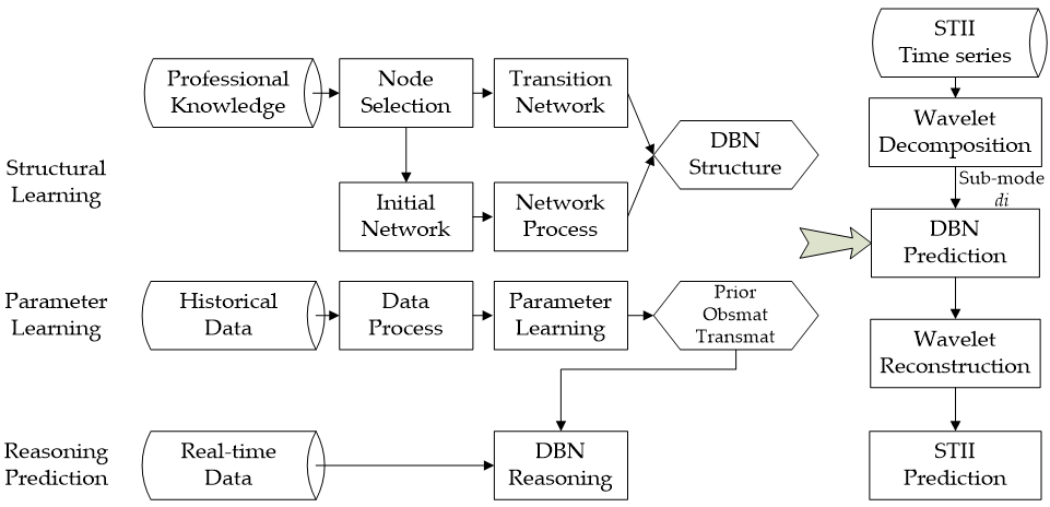
A time-delayed correlation analysis between the above AC indexes and the STII has been made, and the 9 most relevant indexes are chosen as predictors: AL index, AO index, PVI (polar vortex intensity) index, PVA (polar vortex area) index, KI index (Kuroshio SST), NINO index (Niño-3.4 SST), PNA index, SH (Siberian high pressure) index and WP index, respectively denoted as $\mathrm{AL},\mathrm{AO},\mathrm{PVI},\mathrm{PVA},\mathrm{KI},\mathrm{NINO},\mathrm{PNA},\mathrm{SH},$ and $\mathrm{WP}$. The complete DBN node set is:

• Child node set (predictor) = $\left\{\mathrm{AL},\mathrm{AO},\mathrm{PVI},\mathrm{PVA},\mathrm{KI},\mathrm{NINO},\mathrm{PNA},\mathrm{SH},\mathrm{WP}\right\}$
• Parent node set (predictand) = $\left\{\mathrm{STII}\right\}$

3.1.2. Construction of Initial Network and Transition Network

The definition of causality is the premise to express the transfer rules between different nodes. Based on the network nodes and the analysis in Section 3.1.1, we define the following causality:

$$\{\begin{array}{c}P(\mathrm{AL},\mathrm{AO},\mathrm{PVI},\mathrm{PVA},\mathrm{KI},\mathrm{NINO},\mathrm{PNA},\mathrm{SH},\mathrm{WP}|\mathrm{STII})\\ P(\mathrm{STII}\left[\mathrm{t}+1\right]|\mathrm{STII}\left[\mathrm{t}\right])\end{array}$$

Figure 2 shows the DBN topology structure between two adjacent time slices, including the initial network and transition network.

3.2. Parameter Learning

The aim of node parameters determination is to extract the probability distribution from the historical data that truly reflects the causality among variables. The learning steps includes determining the states taken by the node and training parameters by intelligent algorithms. Under the complete historical data, we choose the Expectation-Maximization (EM) algorithm to learn the parameters.

3.2.1. Determination of Node States

As DBN is better at processing discrete data, the continuous data is required to be discretized to determine the number of states taken by the node. We analyze the historical data over a period and discretize the node states according to the maximum and minimum values. Consequently, discrete state space of each node is obtained used the equal interval division method [40].

3.2.2. Calculation of Probability Distribution

First initialize the probability distribution of each node, including prior probability, observation probability, and transition probability. Then, based on the inference mechanism and training data, use EM algorithm to learn parameters and correct the initial probability distribution, to get the probability distribution that matches the objective data. The idea of the EM algorithm is to replace the actual statistics with the expected statistics, whose learning process is iterative and involves two steps:

• E step: Infer the distribution $P(Z|X,{\theta }^t)$ of hidden variable $Z$ with the current parameter ${\theta }^t$ and observed variables $X$, and calculate the expectation of log likelihood $LL({\theta }^t|Z,X)$ for $Z$:

  $$Q\left(\theta |{\theta }^t\right)={\mathrm{E}}_{Z|X,{\theta }^t}\left[LL\left(\theta |X,Z\right)\right],$$

  (2)
• M step: Find the parameter to maximize the expectation likelihood:

  $${\theta }^{t+1}=\mathrm{argmax}\left[Q\left(\theta |{\theta }^t\right)\right].$$

  (3)

3.3. Probabilistic Inference of Prediction Distribution

Based on the DBN structure and node parameters, the probability distribution calculation in the predicted time slice belongs to the probabilistic reasoning problem of BN. Bayesian inference algorithm includes exact algorithm and approximate algorithm. Approximate algorithm is more applied to large-scale network structure to solve the problem of excessive computation. Considering the scale of the network in our research, we apply the exact algorithm-joint tree inference algorithm to accurate reasoning [41]. Each predictor data is input as evidence into the DBN and the joint probability distribution is calculated, then it is marginalized to obtain the prediction distribution of STII.

4. Prediction Experiment of STII

We use the WA-DBN probabilistic prediction model to predict STII and all experiments are performed with MATLAB (R2012a, The MathWorks, Natick, MA, USA). Both the wavelet decomposition and DBN construction are conducted with Wavelet Tool-Box and FullBNT Tool-Box (v1.0.4) [42].

4.1. Data Introduction

In this research, the study area is taken as [30° N–60° N, 120° E–120° W]. Winter data (November to March) of the 500 $\mathrm{hPa}$ geopotential height at a horizontal resolution of 2.5° × 2.5° are obtained from the National Center for Environment Prediction (NECP) and National Center for Atmospheric Research (NCAR) of United States of American for the period 1961–2010. Data sources of the predictors are shown in

Table 1. Data sources of 9 predictors in STII prediction.

Predictor	Data Source
$\mathrm{AO},\mathrm{PNA},\mathrm{WP}$	NOAA Climate Prediction Center
$\mathrm{AL},\mathrm{SH}$	Calculation with sea level pressure data from NCEP/NCAR
$\mathrm{NINO}$	Hadley Center
$\mathrm{KI}$	Calculation with SST data from Hadley Center
$\mathrm{PVI},\mathrm{PVA}$	74 circulation characteristics from the National Climate Center

, and the coverage period is the same. We calculate the STII according to the definition in Section 2.1 and get a single time-series of each variable with 250 months. The first 240 months are chosen as training data and the last 10 months are test data.

4.2. Construction of WA-DBN Prediction Model

4.2.1. Wavelet Decomposition Module

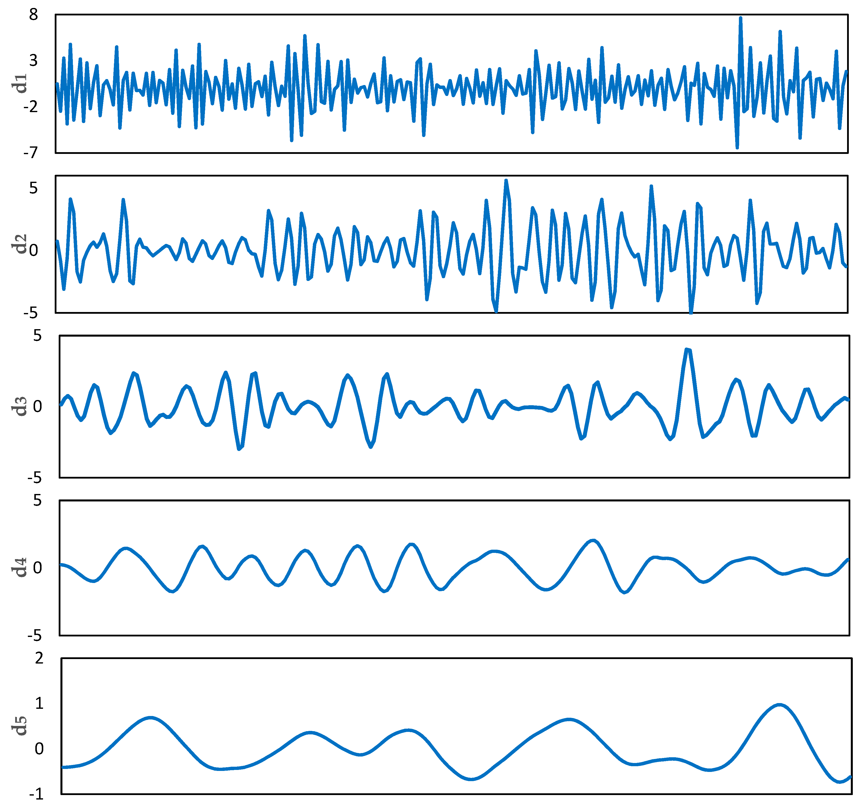
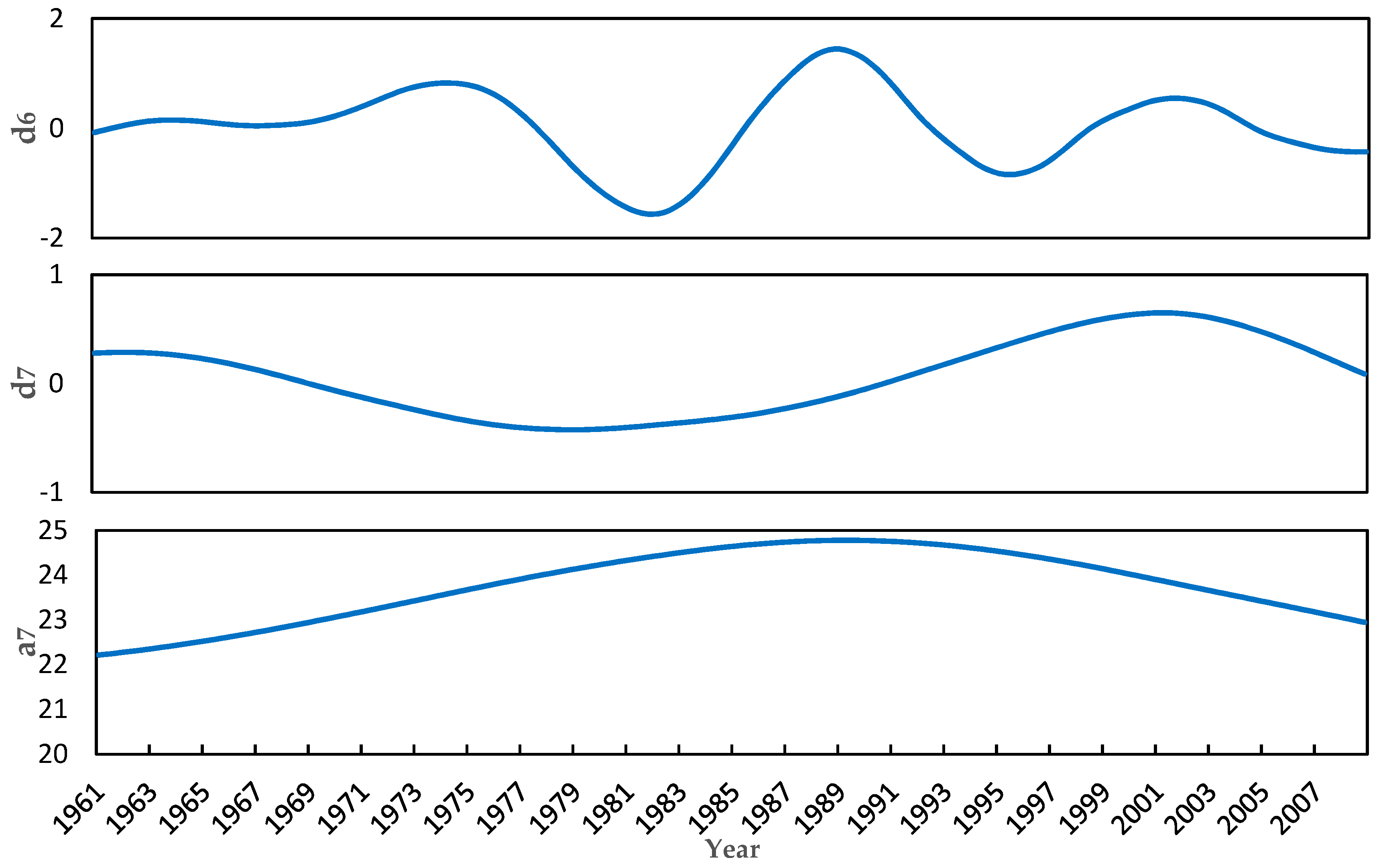
We apply wavelet decomposition to original STII time-series (first 240 months) with Daubechies orthogonal mother wavelet [43]. As a result, a total of seven detailed components and one level of approximation are acquired as shown in Figure 3.

Modes $d_1-d_3$ contain the noise information in the original sequence. $d_4-d_7$ are the detail modes with gradually increasing period and decreasing amplitude, containing the significant information of the original sequence. Mode $a_7$ indicates the linear trend of the original sequence.

4.2.2. DBN Prediction Module

DBN is applied to predict each sub-mode, and the final probabilistic prediction of STII is obtained by integrating each prediction result with a reconstruction algorithm.

(1) Data Process

According to historical records, we select reasonable interval division steps for 9 predictors and 8 sub-modes and denote them with consecutive numbers. The discretization standard is shown in

Table 2. Discretization standard for predictors and modes of STII.

Predictor	Interval Step	State Number	Sub-Mode	Interval Step	State Number
$\mathrm{AL}$	1	1–23	$d_1$	1	1–15
$\mathrm{AO}$	0.1	1–78	$d_2$	1	1–14
$\mathrm{CVI}$	10	1–16	$d_3$	1	1–8
$\mathrm{CVS}$	10	1–29	$d_4$	1	1–6
$\mathrm{KU}$	0.1	1–63	$d_5$	0.1	1–32
$\mathrm{NINO}$	0.1	1–48	$d_6$	0.1	1–20
$\mathrm{PNA}$	0.1	1–46	$d_7$	0.1	1–14
$\mathrm{SH}$	1	1–24	$a_7$	0.1	1–23
$\mathrm{WP}$	0.1	1–59	-	-	-

. Then we discretize the predictors and sub-modes with equal interval to obtain training data of each modes (See Table S1 in Supplementary Material).

(2) Network Construction and Parameter Learning

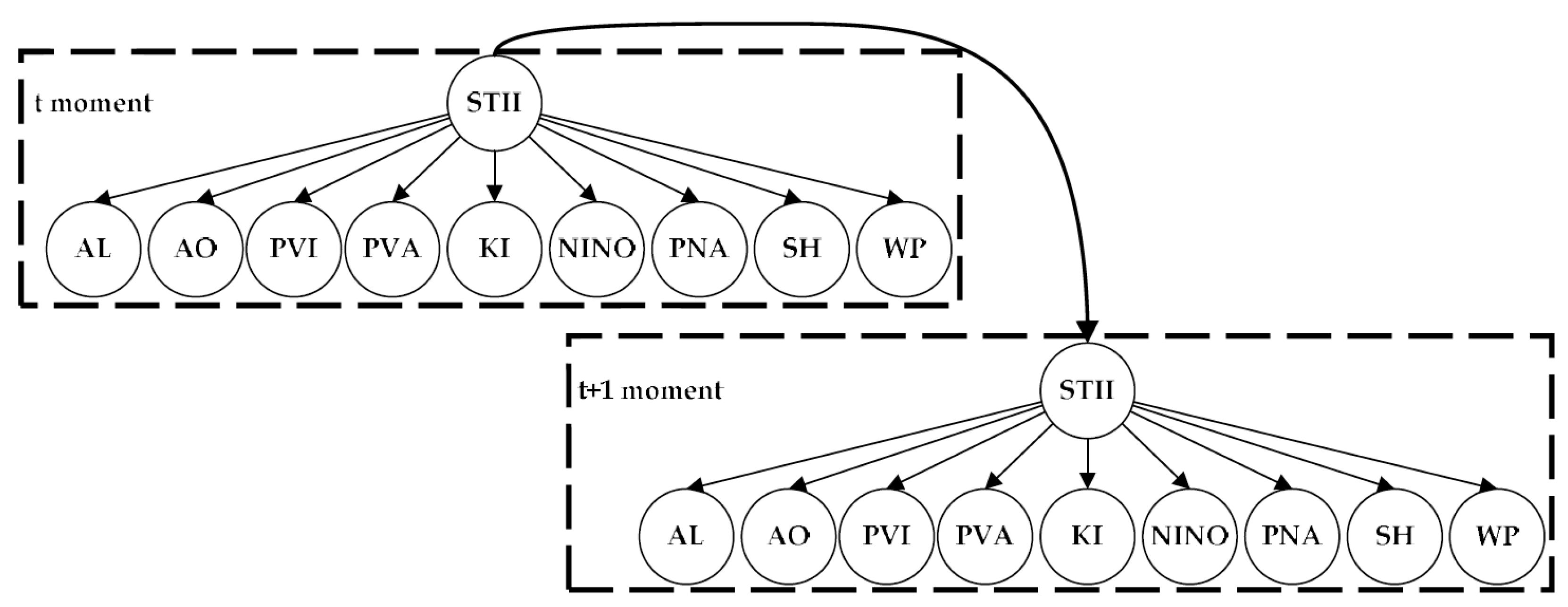
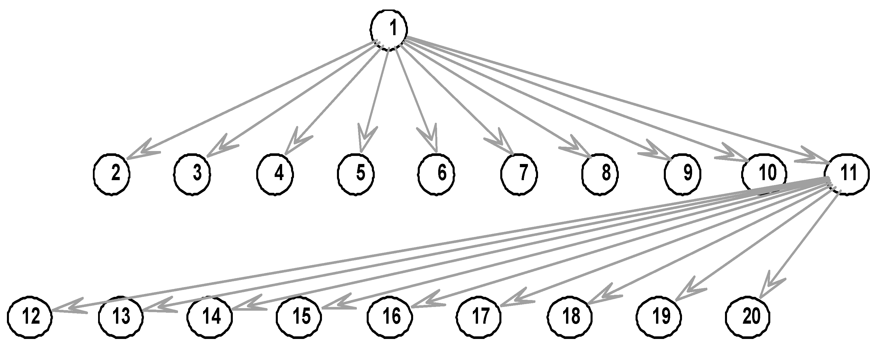
Based on the node variables and causality determined in Section 3.1, the DBN structure is generated with MATLAB. In Figure 4, Node 1 denotes each sub-mode ($d_1-d_7,a_7$) of the predictand (STII) and nodes 2–10 denote predictors. Nodes 1–10 are in the previous time slice while nodes 11–20 are in the latter time slice.

After constructing the network structure, EM algorithm is used to learn parameters, i.e., the prior probability, conditional probability, and transition probability of the nodes. Where the transition probability is shown in

Table A1. Transition probability of DBN (Take $d_1$ as an example).

	${\mathit{d}}_1$[t + 1]	State of Node ${\mathit{d}}_1$
${\mathit{d}}_1$[t]		1	2	3	4	5	6	7	8	9	10	11	12	13	14	15
State of node $d_1$	1	0.0216	0.0945	0.1261	0.1034	0.0300	0.0595	0.0333	0.0457	0.0209	0.0958	0.0333	0.1433	0.1069	0.0584	0.0273
	2	0.0487	0.0265	0.0237	0.0810	0.0257	0.0496	0.0363	0.0754	0.0622	0.1089	0.1322	0.2414	0.0000	0.0566	0.0874
	3	0.0842	0.1204	0.0061	0.0595	0.0674	0.0458	0.0340	0.0480	0.0532	0.1058	0.0574	0.1593	0.0159	0.0008	0.1423
	4	0.0421	0.1065	0.0759	0.1251	0.0434	0.0118	0.0462	0.0096	0.0063	0.0342	0.0422	0.0354	0.2644	0.0366	0.1205
	5	0.1011	0.0469	0.0006	0.0646	0.1125	0.0172	0.0694	0.0489	0.0483	0.0318	0.1656	0.1431	0.0470	0.0471	0.0559
	6	0.0479	0.0060	0.0366	0.0047	0.0732	0.0311	0.0829	0.0797	0.0438	0.0317	0.0646	0.1056	0.1533	0.1685	0.0702
	7	0.0451	0.0016	0.0262	0.0149	0.0298	0.0298	0.0019	0.0822	0.0874	0.1250	0.0742	0.1462	0.1862	0.1423	0.0072
	8	0.0191	0.0483	0.0018	0.0752	0.0501	0.0122	0.0939	0.0515	0.1213	0.1363	0.0483	0.1239	0.0036	0.0770	0.1375
	9	0.0211	0.0464	0.0224	0.0443	0.0304	0.0675	0.0985	0.0492	0.0097	0.0161	0.0639	0.0672	0.2843	0.1767	0.0024
	10	0.0119	0.0605	0.0650	0.0593	0.0031	0.0474	0.0364	0.0084	0.0348	0.0095	0.0440	0.2152	0.2097	0.0148	0.1800
	11	0.0581	0.0558	0.0032	0.0264	0.0573	0.0028	0.0267	0.0368	0.1084	0.0731	0.0208	0.0334	0.1295	0.0685	0.2992
	12	0.0567	0.0078	0.0159	0.0021	0.0802	0.0649	0.0204	0.0409	0.0775	0.0919	0.0118	0.0424	0.0538	0.4025	0.0312
	13	0.0348	0.0121	0.0473	0.0070	0.0004	0.0506	0.0356	0.0518	0.0356	0.0809	0.0473	0.0013	0.3053	0.1681	0.1219
	14	0.0531	0.0196	0.0071	0.0205	0.0525	0.0559	0.0140	0.0470	0.0966	0.0154	0.1670	0.2083	0.0627	0.0790	0.1014
	15	0.0544	0.0269	0.0920	0.0293	0.0875	0.0058	0.0046	0.0054	0.0501	0.1055	0.0522	0.1092	0.2252	0.0271	0.1248

in Appendix A.

4.3. Reasoning Prediction and Result Analysis

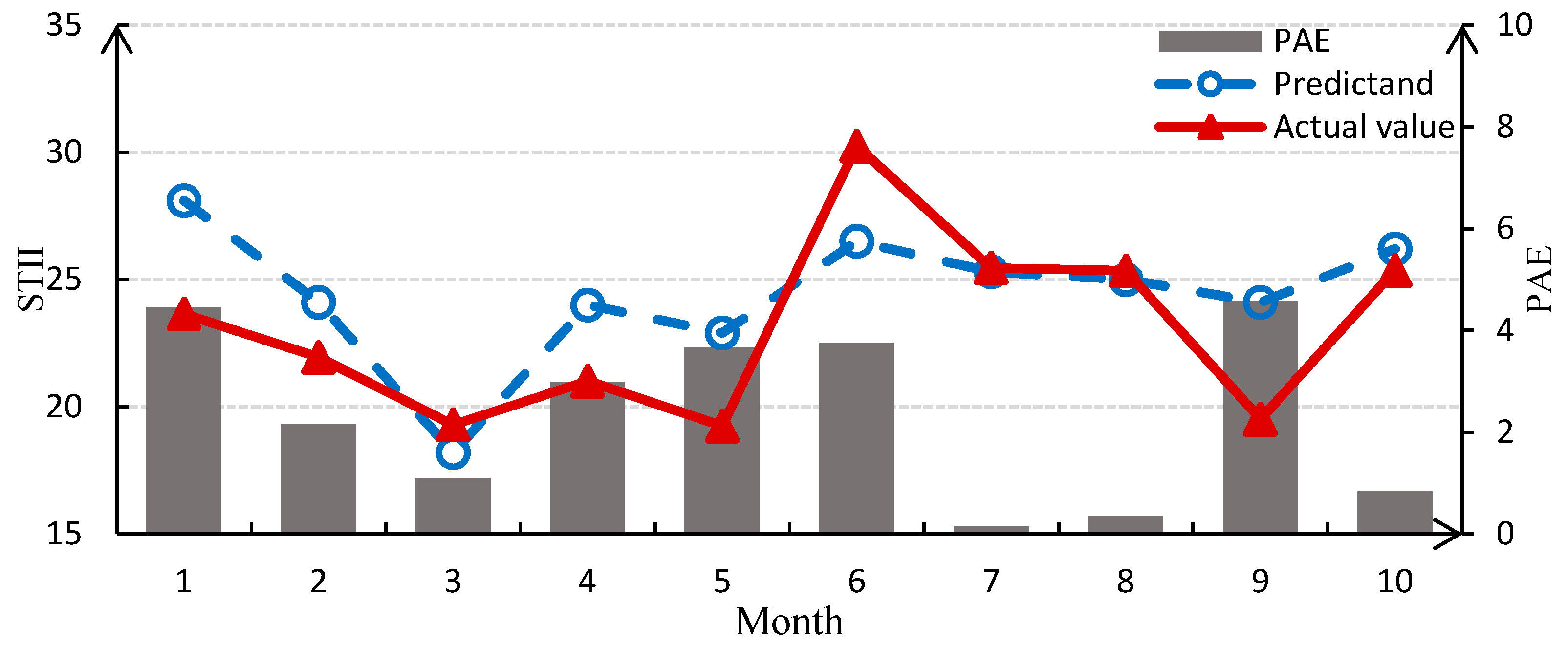
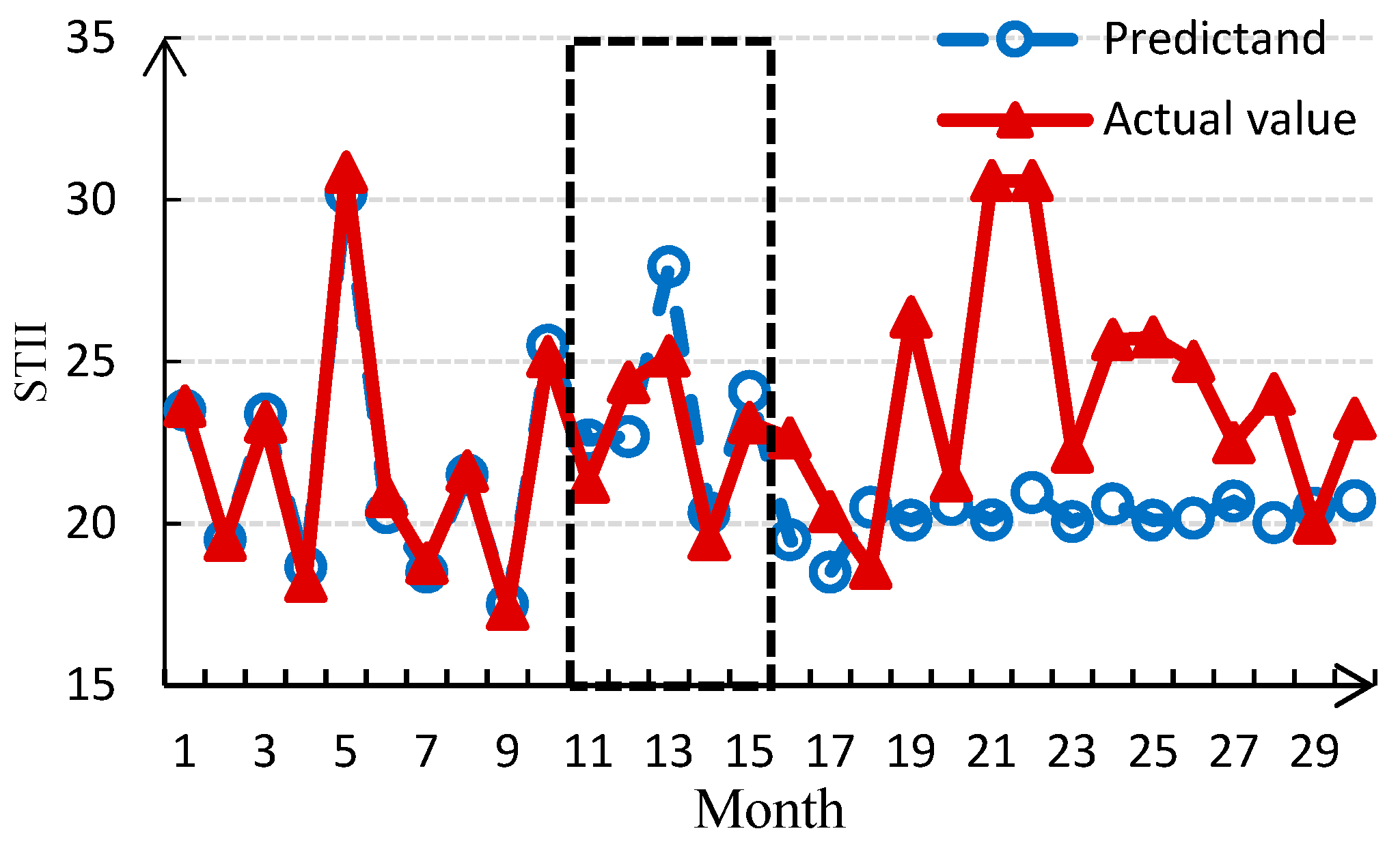
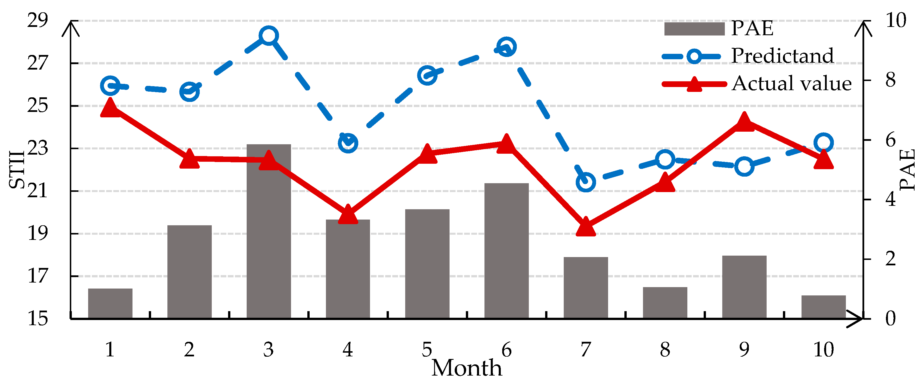
Following the determination of structure and parameters, we discretize the test data of predictors (later 10 months) according to Table 2 and input the discrete value into DBN to reason and predict the probability distribution of each sub-mode in the last 10 months. The results are shown in

Table A2. Monthly predicted probability distribution of $d_1$ (The maximum probability of probability distribution for each month is highlighted).

	Month	1	2	3	4	5	6	7	8	9	10
State
1		1.77 × 10−31	1.84 × 10−22	2.58 × 10−38	7.61 × 10−28	4.06 × 10−33	1.96 × 10−32	5.13 × 10−31	2.42 × 10−31	2.75 × 10−34	1.44 × 10−35
2		4.30 × 10−15	6.15 × 10−25	9.92 × 10−30	1.16 × 10−9	5.74 × 10−23	1.62 × 10−21	2.34 × 10−13	1.86 × 10−30	2.09 × 10−21	1.18 × 10−27
3		1.23 × 10−8	2.95 × 10−7	1.30 × 10−26	1.78 × 10−12	1.42 × 10−14	3.85 × 10−22	1.48 × 10−15	3.50 × 10−15	1.23 × 10−5	4.82 × 10−8
4		3.71 × 10−5	0.96607572	1.86 × 10−10	0.04711185	1.99 × 10−8	4.68 × 10−12	3.71 × 10−9	1.30 × 10−11	9.51 × 10−8	6.19 × 10−6
5		1.15 × 10−9	0.00024291	1.51 × 10−8	3.08 × 10−5	0.61559523	1.19 × 10−7	1.18 × 10−7	0.00059951	0.00021533	0.7366376
6		0.00017127	0.03368107	0.99670829	8.29 × 10−5	0.35914973	0.13090291	2.02 × 10−5	0.99737456	0.99907177	0.18456279
7		0.99968979	9.37 × 10−12	3.18 × 10−6	0.12481569	0.00022297	0.00131173	0.99986409	4.70 × 10−9	0.00070003	0.00034761
8		0.00010175	1.07 × 10−12	2.85 × 10−19	7.14 × 10−5	1.30 × 10−5	0.86778512	6.07 × 10−5	2.12 × 10−15	1.59 × 10−14	4.45 × 10−13
9		2.23 × 10−8	1.89 × 10−15	0.00328851	0.82788733	0.0250191	1.14 × 10−7	8.20 × 10−9	0.00202593	4.30 × 10−7	0.07844577
10		5.79 × 10−8	9.98 × 10−27	1.97 × 10−15	1.45 × 10−12	2.37 × 10−13	3.61 × 10−19	5.49 × 10−5	1.01 × 10−14	1.10 × 10−18	1.92 × 10−15
11		9.39 × 10−24	6.20 × 10−31	6.15 × 10−30	1.18 × 10−31	2.45 × 10−25	2.17 × 10−18	2.93 × 10−27	1.45 × 10−33	6.63 × 10−33	4.81 × 10−31
12		1.82 × 10−18	3.21 × 10−35	1.52 × 10−32	4.61 × 10−29	2.24 × 10−21	1.40 × 10−31	3.40 × 10−29	8.46 × 10−35	4.39 × 10−21	8.99 × 10−28
13		2.66 × 10−27	1.18 × 10−30	1.63 × 10−37	4.44 × 10−23	8.72 × 10−31	1.06 × 10−31	5.38 × 10−30	1.75 × 10−33	2.64 × 10−24	9.63 × 10−31
14		1.77 × 10−31	2.35 × 10−35	2.58 × 10−38	1.50 × 10−32	1.43 × 10−35	8.70 × 10−35	1.17 × 10−31	7.75 × 10−35	2.75 × 10−34	5.76 × 10−36
15		1.75 × 10−26	2.35 × 10−35	2.29 × 10−29	1.50 × 10−27	1.43 × 10−30	8.70 × 10−35	1.17 × 10−21	7.87 × 10−30	5.63 × 10−29	5.76 × 10−31

in Appendix A. Take the median of the most probable interval as the predictand of each sub-mode, then apply the wavelet reconstruction to get the composite predictand of STII. Figure 5 plots the monthly predicted and actual STII in the test period together with the prediction absolute error (PAE) yield of the WA-DBN model for each tested month.

At present, most of the common evaluation indicators for prediction accuracy in the literature are the following: average sum error, average absolute error, average relative error, root mean square error, etc. [44]. All of them can measure the deviation between the predicted value and the actual value.

To statistically test the performance of WA-DBN model, three prediction score metrics are employed: root mean square error (RMSE), mean relative error (MRE) and correlation coefficient (R). The RMSE of the prediction result is 2.8954, the MRE is 0.0794, and the R value is 0.6579. The prediction variation of the STII is less and the changing tendency agrees with that in reality.

Different from previous prediction models, the WA-DBN model could provide a casual graph and conditional probability. Therefore, it can intuitively and quantitatively express the relationship between STII and climate indexes, which could deal with the uncertainty and nonlinearity to improve prediction accuracy. In contrast with the certain mapping relationship, the model could establish the probabilistic mapping between predictands and predictors and offer the comprehensive prediction information with probability distribution.

5. Model Analysis and Discussion

To make a further test for the WA-DBN prediction model, we conduct another prediction experiment, the regression fitting experiment, and the comparison experiment with NN and Poisson regression (P-regression). Moreover, the error analysis of the prediction results is performed and discussed.

5.1. Model Experiment and Discussion

5.1.1. Prediction Experiment

(1) Contrast experiment with the Poisson regression

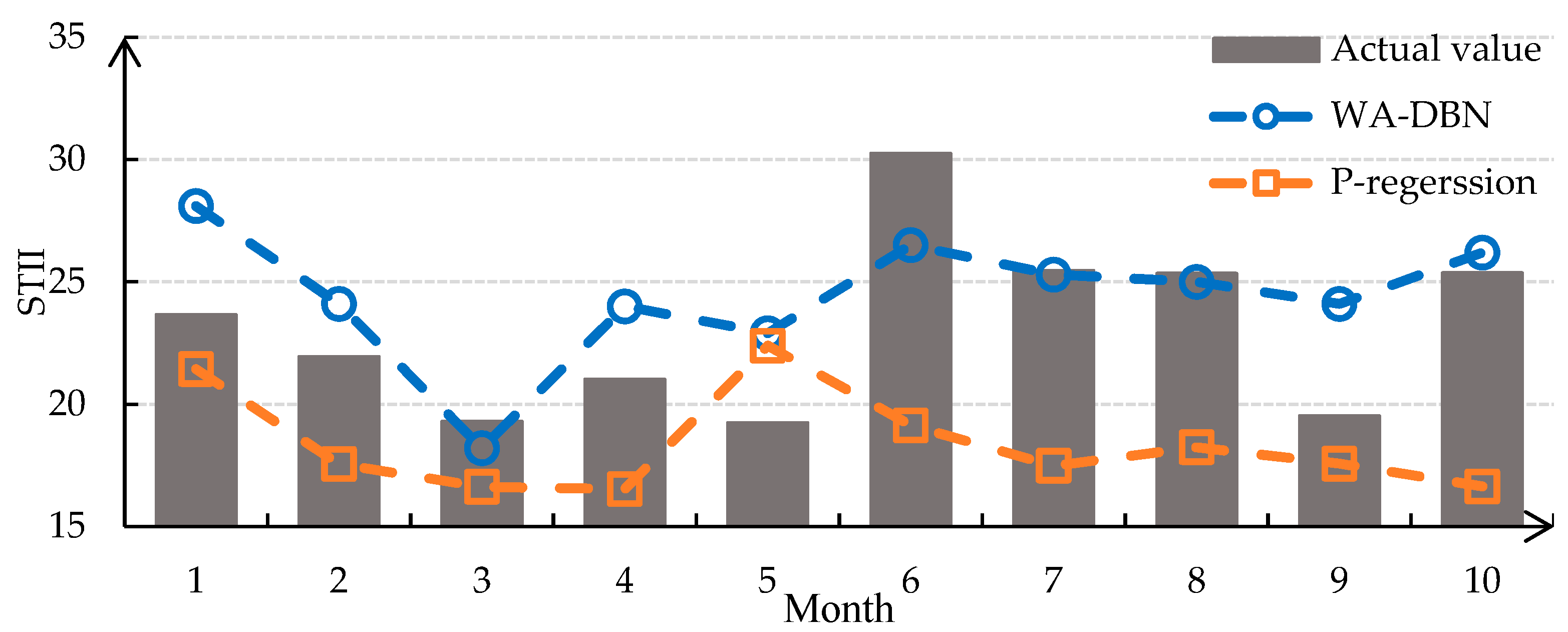
To test the prediction capacity of this model, a prediction experiment with the classic P-regression is conducted for comparison [44]. We also use the first 240 months for training and the last 10 months for predicting in Section 4. Figure 6 and

Table 3. Error analysis of WA-DBN and P-regression.

	Indicator	RMSE	MRE	R
Model
WA-DBN		2.8954	0.0794	0.6579
P-regression		6.1703	0.1778	0.1981

show the comparative results and error analysis. As evidence by higher R and smaller RMSE, the WA-DBN model has better prediction ability than P-regression.

(2) Prediction experiment with different training samples

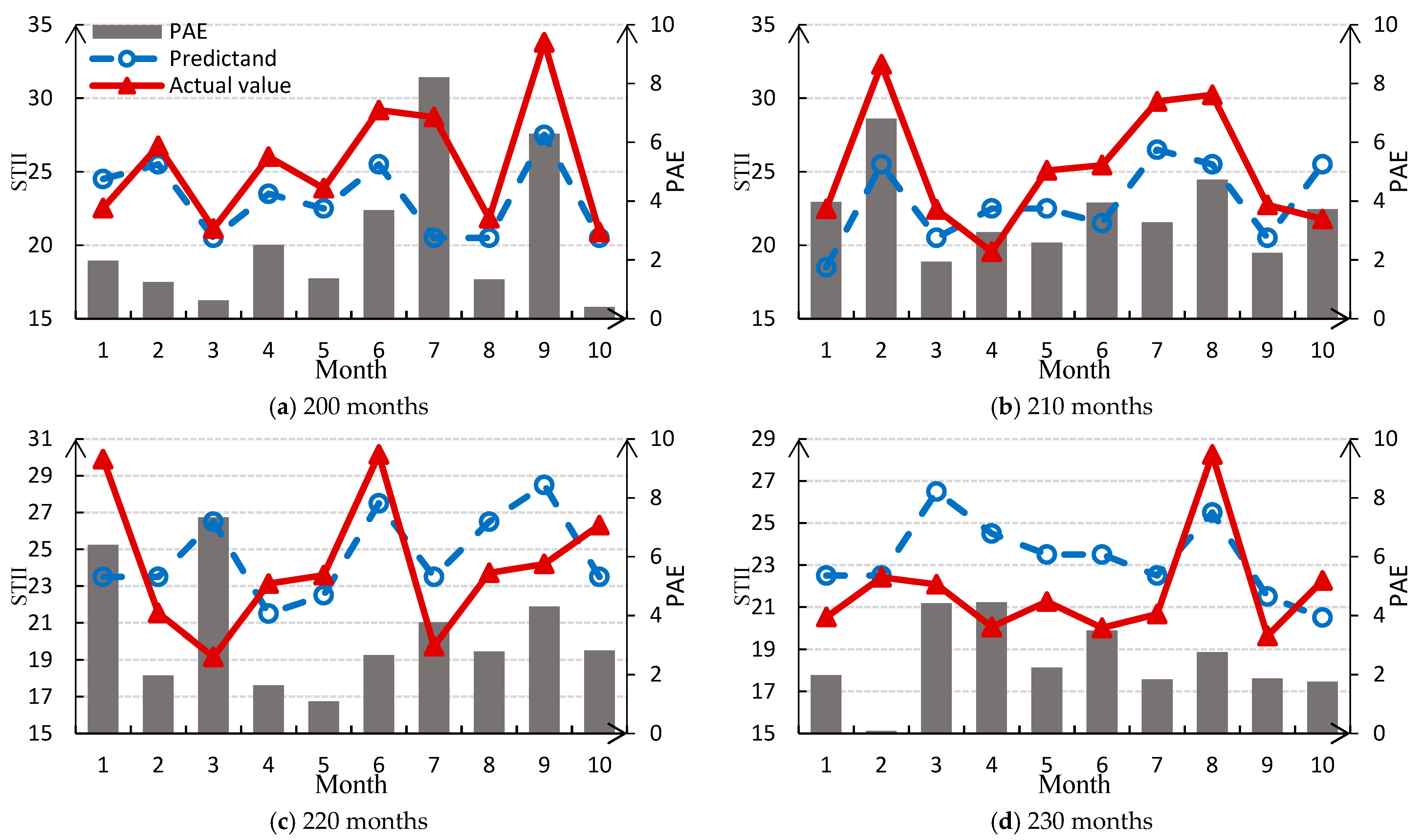
In accordance with the experiment steps in Section 4, we use 4 sets of data with different time-series length (i.e., 200 months, 210 months, 220 months, and 230 months) to train the model respectively, then successively predict for 10 months. The prediction result is shown in Figure 7 and error analysis is shown in

Table 4. Error analysis of WA-DBN prediction model with different training data.

	Training Data	200 Months	210 Months	220 Months	230 Months	Mean
Indicator
RMSE		3.6956	3.8548	3.9734	2.7921	3.5789
MRE		0.0818	0.1119	0.1152	0.0881	0.0993
R		0.6341	0.6806	0.5245	0.5346	0.5935

.

The RMSE of four groups of prediction results are all around 3.5, MRE is around 0.1, and R is around 0.6, indicating that the model has good prediction accuracy, good correlation, and high stability. More importantly, the prediction of extremums is more accurate, which is meaningful for ST prediction. However, there are also outliers of predictions, such as the large deviations in the prediction results from month 6 to 7 in Figure 7a and from month 1 to 3 in Figure 7c.

5.1.2. Fitting Experiment

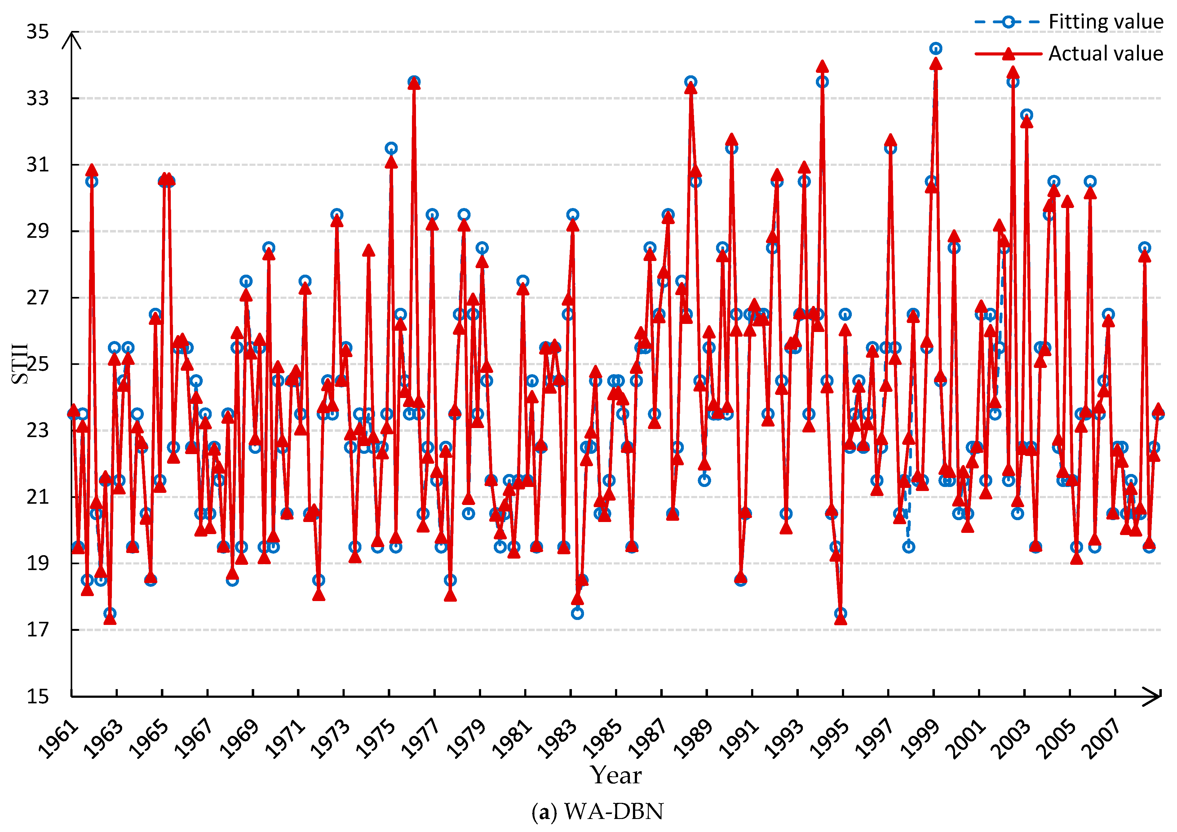
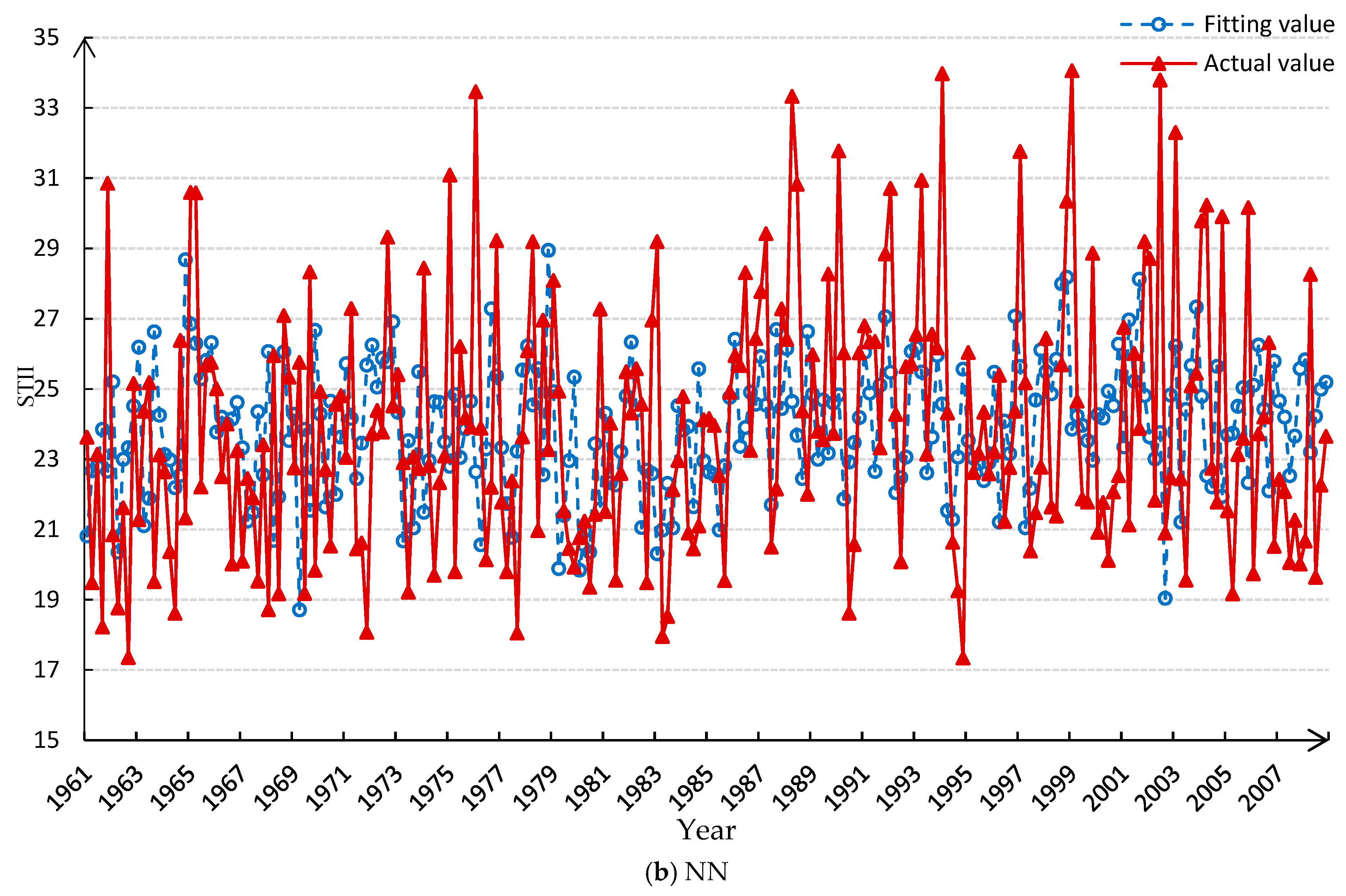
We train the model with the first 240-month data and input the corresponding predictor data for return fitting, comparing the fitting result with NN [45]. The comparison result and error analysis are shown in Figure 8 and

Table 5. Error analysis of WA-DBN and NN.

	Indicator	RMSE	MRE	R
Model
WA-DBN		3.7311	0.2315	0.9771
NN		18.7454	2.1849	0.2237

.

From Table 5, the single-point fitting accuracy with the WA-DBN probabilistic prediction model is significantly better than the deterministic NN method. When there are large fluctuations in the data, the error increases significantly for NN, but the DBN can give a probability distribution relatively close to the reality according to the transition between different states of the STII in the historical data. All states of STII are presented in the probability distribution without loss of results.

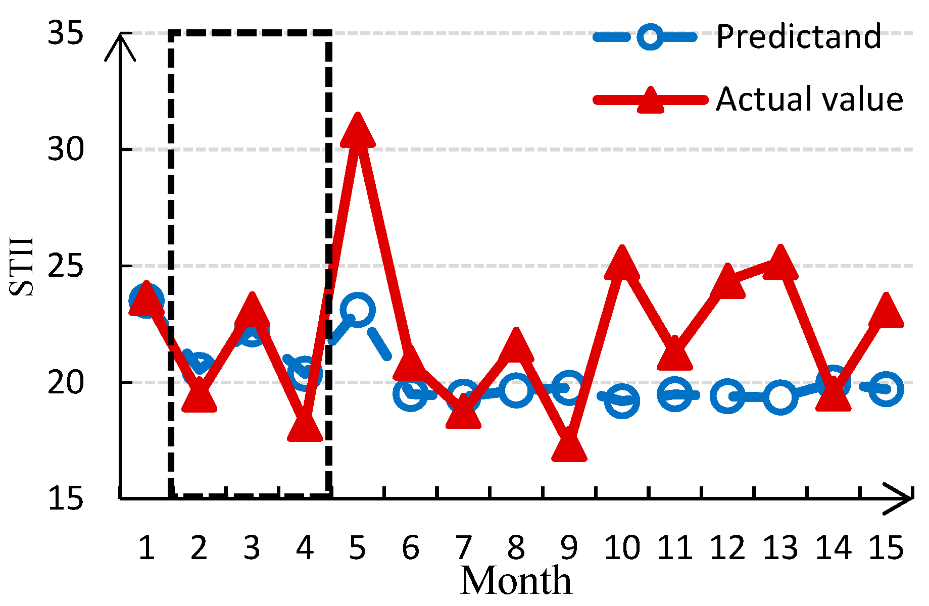
To further test the time-validity of WA-DBN model over short- and long-term prediction, we input the first month data and the first 10-month data of predictors when performing regression fitting experiments. Figure 9 (a) indicates that only the first month data is input, the results of the subsequent three months are more effective, but the other predictions have greater errors; (b) indicates that when input the first 10-month data, the results of the subsequent five months are more effective. Although the predictable time extends when the input time is increased from 1 to 10 months, the predictable time is still short. Thus, the model is not suitable for medium- and long-term prediction. The reason may be that the probabilistic inference of DBN depends on the priori probability of nodes. When only the finite priori probability is given, such as one month or ten months, the reasoning error increases as the predicted time increases.

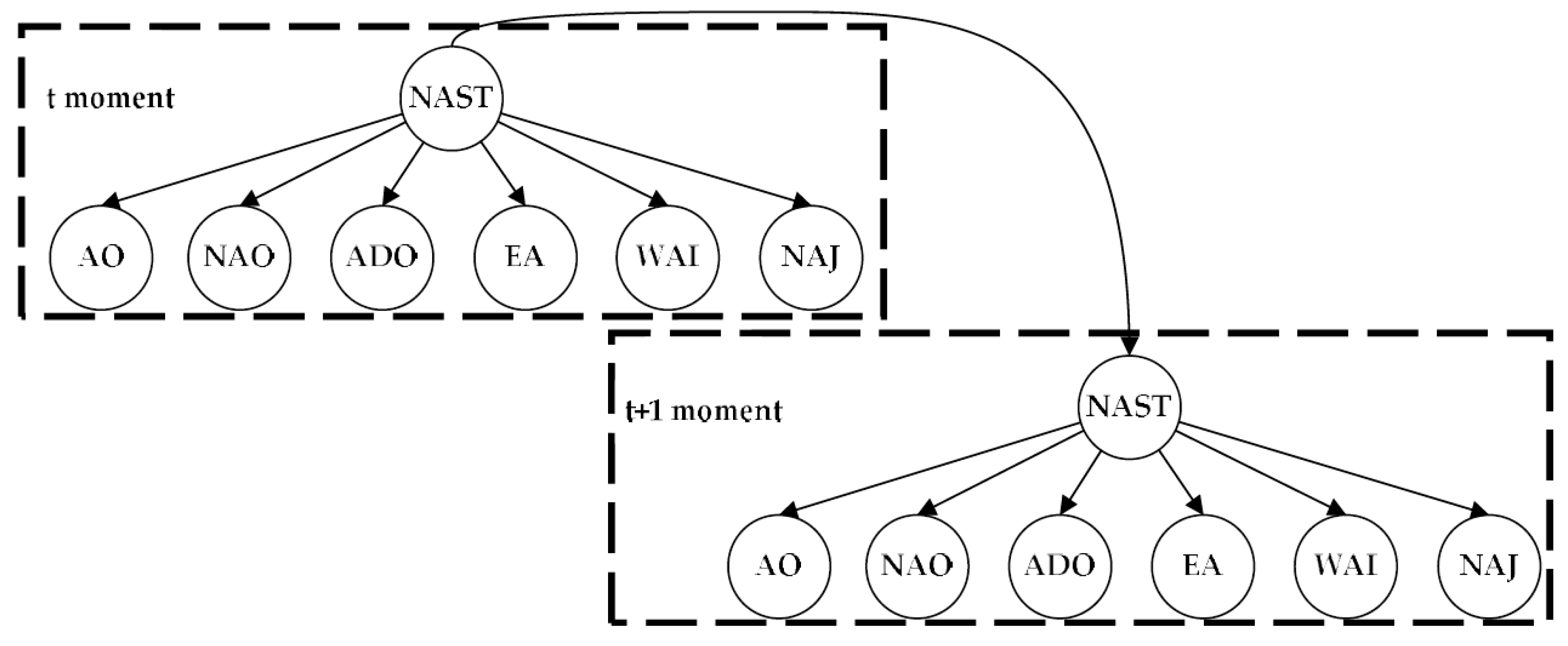
5.1.3. Expending Experiment for NAST Intensity Index Prediction

To further verify the generalization ability of this model, we perform a prediction experiment of NAST (35° N–70° N, 90° W–0° W). The NAST intensity index is also calculated with the same definition in Section 2.1. A time-delayed correlation analysis between the AC indexes [46] and the NAST intensity index has also been made. Different from NPST, 6 most relevant indexes are chosen as predictors: AO index, North Atlantic Oscillation (NAO) index, Atlantic Decadal Oscillation (ADO) index, East Atlantic (EA) index, West Atlantic index (WAI), and North American Jet Stream (NAJ) index, respectively denoted as $\mathrm{AO},\mathrm{NAO},\mathrm{ADO},\mathrm{EA},\mathrm{WAI}$ and $\mathrm{NAJ}$. The DBN network with above nodes is constructed as shown in Figure 10.

According to the integrated steps in Section 4, we conduct the same prediction experiment of NAST. Figure 11 displays the monthly predicted intensity index of NAST.

We calculate the evaluation indicators for prediction accuracy: the RMSE is 3.1717, the MRE is 0.1104, and the R value is 0.5568. Therefore, it is reasonable to generalize the WA-DBN model for other mid-latitude ST regions and the predicted results are reliable. This prediction model has adaptive ability owing to the flexible modeling features of DBN.

6. Conclusions

Effective short-term prediction of STII is significant for researches of mid-latitude weather systems, especially the analysis of abnormal changes. In this study, we have applied the state-of-the art artificial intelligence to predict the monthly intensity index of NPST with WA-DBN probabilistic prediction model. Considering the non-stationarity, nonlinearity, and uncertainty of the STII time-series, we first used the WA to decompose the intensity index into the sub-modes with different frequency domains. Then we applied the DBN to make a probabilistic prediction for each sub-mode. Finally, the independent prediction results of each mode were integrated with the wavelet reconstruction.

To further illustrate the advantages of the model, we conducted multiple sets of STII prediction experiments, fitting experiments, and comparison experiments. The results show that predicting correlation coefficient reached about 0.6 and fitting correlation coefficient reached 0.97. Moreover, this model is good at predicting extremums. Therefore, the WA-DBN model exhibits relatively better performance in prediction of nonlinear uncertainties, as evidence by higher R and smaller RMSE. The improved performance of the WA-DBN model is attributable to two aspects:

• The input dataset of predictand is decomposed into separate components based on different frequencies with WA, allowing removal of noisy data and revealing the quasi-periodic components in the original time-series.
• Both the relationship between the predictand and the predictors at the same time and that in adjacent time slices are considered with DBN model. The expression of casual relationship with network structure and probability distribution can better deal with the uncertainty of prediction.

We summarize that the WA-DBN model developed and tested in this study has good prediction skills of monthly STII, which is of great scientific guidance to study the abnormal changes of ST and its mechanisms. Above all, we propose a new intelligent prediction model based on graph theory and probability theory, which has wide application prospects with strong generalization ability and good stability.

Although the WA-DBN probabilistic predicting model works well, there are still some problems. First, the selection of the predictors of the ST intensity index needs to be further improved. The existing studies indicate that if the number of predictors exceeds 10, the predicting calculation will be complex, and the accuracy will not increase significantly with more predictors. If fewer predictors are selected such as 5, the accuracy will become poor due to loss of information. In this research, we chose 9 most relevant indicators as predictors. However, the selection of predictors is crucial to prediction, and we need to improve this work. Second, the accuracy of the long-term prediction in this model is low. These are also the focus of future work.

References

- Blackmon, M.L. A Climatological Spectral Study of the 500 mb Geopotential Height of the Northern Hemisphere. J. Atmos. Sci. 1976, 33, 1607–1623. [Google Scholar] [CrossRef] [Green Version]
- Zhu, W.J.; Li, Y. Characteristics of the interdecadal variability of the North Pacific storm track and its possible influencing mechanism. J. Meteorol. 2010, 68, 477–486. [Google Scholar]
- Lau, N.C. Variability of the observed midlatitude storm tracks in relation to low-frequency changes in the circulation pattern. J. Atmos. Sci. 1988, 45, 2718–2743. [Google Scholar] [CrossRef]
- Straus, D.M.; Shukla, J. Variations of midlatitude transient dynamics associated with ENSO. J. Atmos. Sci. 1997, 54, 777–790. [Google Scholar] [CrossRef]
- Zhu, W.J.; Sun, Z.B. Interannual variation of the North Pacific storm track in winter and its relationship with 500hPa height and SST in the Tropical and North Pacific Oceans. Acta Meteorol. Sin. 2000, 58, 309–320. [Google Scholar]
- Ren, X.J.; Yang, X.Q.; Han, B. Variation characteristics of the North Pacific storm track and its coupling with mid-latitude ocean-atmosphere. Chin. J. Geophys. 2007, 50, 92–100. [Google Scholar] [CrossRef]
- Liu, M.Y.; Zhu, W.J.; Gao, J. Effect of Northern Hemisphere polar vortex intensity on North Pacific storm track. Chin. J. Atmos. Sci. 2013, 36, 297–308. [Google Scholar]
- Sun, Z.B.; Zhu, W.J. A modelling study of Northwest Pacific SSTA effect on Pacific storm track during winter. J. Meteorol. Res. 2000, 14, 416–425. [Google Scholar]
- Zhu, W.J.; Yuan, K.; Chen, Y.N. The temporal and spatial evolution of the storm track in the eastern North Pacific Ocean. Chin. J. Atmos. Sci. 2013, 37, 65–80. [Google Scholar]
- Ding, Y.F.; Ren, X.J.; Han, B. A Preliminary study on the climate characteristics and changes of the North Pacific storm track. Sci. Meteorol. Sin. 2006, 26, 237–243. [Google Scholar]
- Li, Y.; Zhu, W.J.; Wei, J.S. Assessment and improvement of the North Pacific storm track index in winter. Chin. J. Atmos. Sci. 2010, 34, 1001–1010. [Google Scholar]
- Hong, M.; Zhang, R.; Wu, G.X. Nonlinear dynamic model for reconstruction of subtropical high-pressure characteristic index using genetic algorithm. Chin. J. Atmos. Sci. 2007, 31, 164–170. [Google Scholar]
- Liu, K.F.; Zhang, R.; Hong, M. Prediction model of subtropical high based on least square support vector machines. J. Appl. Meteorol. 2009, 20, 354–359. [Google Scholar]
- Zhu, H.R.; Jiang, Z.H.; Zhang, Q. MJO index prediction model experiment Based on SSA-AR model. J. Trop. Meteorol. 2010, 26, 371–378. [Google Scholar]
- Jia, Y.J.; Hu, Y.J.; Zhong, Z. Statistical forecasting model of summer subtropical high in the Western Pacific. Plateau Meteorol. 2015, 34, 1369–1378. [Google Scholar]
- Yang, X.F. Research on Biomedical Data Processing Method Based on Machine Learning. Master’s Thesis, University of Chinese Academy of Sciences, Huairou, China, 2014. [Google Scholar]
- Li, F.; Han, Z.H.; Feng, E.Y. Analysis of financial data based on machine learning. Sci. Wealth 2016, 6, 65–72. [Google Scholar]
- Qin, Y.B. Design of medical learning medical diagnosis and treatment system based on the core thinking of traditional Chinese medicine. Chin. J. Tradit. Chin. Med. 2015, 52, 2188–2191. [Google Scholar]
- Yang, R.; Tang, J.; Sun, D. Association rule data mining applications for Atlantic tropical cyclone intensity changes. Weather Forecast. 2010, 26, 337–353. [Google Scholar] [CrossRef]
- Royston, S.; Lawry, J.; Horsburgh, K. A linguistic decision tree approach to predicting storm surge. Fuzzy Sets Syst. 2013, 215, 90–111. [Google Scholar] [CrossRef]
- Reikard, G. Combining frequency and time domain models to forecast space weather. Adv. Space Res. 2013, 52, 622–632. [Google Scholar] [CrossRef]
- Teng, W.P.; Hu, B.; Teng, Z. Application of SVM regression in Western Pacific tropical cyclone route forecasting. Sci. Bull. 2012, 28, 49–53. [Google Scholar]
- Yu, J.; Song, Z.; Kusiak, A. Very short-term wind speed forecasting with Bayesian structural break model. Renew. Energy 2013, 50, 637–647. [Google Scholar]
- Voyant, C.; Darras, C.; Muselli, M. Bayesian rules and stochastic models for high accuracy prediction of solar radiation. Appl. Energy 2014, 114, 218–226. [Google Scholar] [CrossRef] [Green Version]
- Li, Y.; Zhu, W.J. Performance comparison of different digital filtering methods in the study of storm track. Chin. J. Atmos. Sci. 2009, 32, 565–573. [Google Scholar]
- Zhou, Z.H. Machine Learning; Tsinghua University Press: Beijing, China, 2016. [Google Scholar]
- Cussens, J. Bayesian network learning with cutting planes. arXiv, 2012; arXiv:1202.3713. [Google Scholar]
- Mallat, S. A Wavelet Tour of Signal Processing; China Machine Press: Beijing, China, 2010. [Google Scholar]
- Wang, N.; Lu, C. Two-dimensional continuous wavelet analysis and its application to meteorological data. J. Atmos. Ocean. Technol. 2010, 27, 652–666. [Google Scholar] [CrossRef]
- Jin, F.R.; Wang, W.R. Analysis and simulation of meteorological wind fields based on wavelet transform. Appl. Mech. Mater. 2014, 490–491, 1228–1236. [Google Scholar] [CrossRef]
- Limpasuvan, V.; Jeev, K.; Hartmann, D.L. Anomalous vortex intensification and associated stratosphere-troposphere evolution. In AGU Fall Meeting Abstracts; American Geophysical Union: Washington, DC, USA, 2004. [Google Scholar]
- Gao, Q. The Spatio-Temporal Evolution of the North Pacific Storm Track in Winter and Its Relationship with AO. Master’s Thesis, Nanjing University of Information Science and Technology, Nanjing, China, 2006. [Google Scholar]
- Gu, P.X. Relationship between the North Pacific Storm Track and East Asian Winter Monsoon. Master’s Thesis, Nanjing University of Information Science & Technology, Nanjing, China, 2013. [Google Scholar]
- Athanasiadis, P.; Wallace, J.M.; Wettstein, J.J. Patterns of jet stream wintertime variability and their relation to the storm tracks. J. Atmos. Sci. 2009, 67, 1361–1381. [Google Scholar] [CrossRef]
- Chang, E.K. Interdecadal variations in Northern Hemisphere winter storm track intensity. J. Clim. 2002, 15, 642–658. [Google Scholar] [CrossRef]
- Tan, B.; Wen, C. Progress in the study of the dynamics of extratropical atmospheric teleconnection patterns and their impacts on East Asian climate. J. Meteorol. Res. 2014, 28, 780–802. [Google Scholar] [CrossRef]
- Mächel, H.; Kapala, A.; Flohn, H. Behaviour of the centres of action above the Atlantic since 1881. Part I: Characteristics of seasonal and interannual variability. Int. J. Climatol. 2015, 18, 1–22. [Google Scholar] [CrossRef]
- Wettstein, J.J.; Wallace, J.M. Observed patterns of month-to-month storm-track variability and their relationship to the background flow. J. Atmos. Sci. 2010, 67, 1420–1437. [Google Scholar] [CrossRef]
- Yang, D.X. A decadal abruption of midwinter storm tracks over North Pacific from 1951 to 2010. Atmos. Ocean. Sci. Lett. 2016, 9, 235–245. [Google Scholar] [CrossRef]
- Hong, W.U.; Wang, W.P.; Feng, Y. Discretization method of continuous variables in Bayesian network parameter learning. Syst. Eng. Electron. 2012, 34, 2157–2162. [Google Scholar]
- Liao, W.; Zhang, W.; Ji, Q. A factor tree inference algorithm for Bayesian networks and its applications. In Proceedings of the 16th IEEE International Conference on Tools with Artificial Intelligence, Boca Raton, FL, USA, 15–17 November 2004; pp. 652–656. [Google Scholar]
- FullBNT-1.0.4. Available online: https://download.csdn.net/download/b08514/6942975 (accessed on 3 June 2018).
- Huang, W.Q.; Dai, Y.X.; Quan, H.M. Harmonic analysis algorithm based on Daubechies wavelet. Chin. J. Electr. Eng. 2006, 21, 45–46. [Google Scholar]
- Bai, C.Z.; Zhang, R.; Bao, S.L. Forecasting the tropical cyclone genesis over the Northwest Pacific through identifying the casual factors in the cyclone-climate interactions. J. Atmos. Ocean. Technol. 2018, 35, 247–258. [Google Scholar] [CrossRef]
- Deo, R.C.; Şahin, M. Application of the artificial neural network model for prediction of monthly standardized precipitation and evapotranspiration index using hydrometeorological parameters and climate indices in eastern Australia. Atmos. Res. 2015, 161–162, 65–81. [Google Scholar] [CrossRef]
- Zhou, X.Y.; Zhu, W.J.; Gu, C. The possible impact of winter north Atlantic storm track anomaly on cold wave activity of China. Atmos. Sci. 2015, 39, 978–990. [Google Scholar]
Figure 1.
Technical structure of WA-DBN probabilistic prediction model.
Figure 2.
DBN structure between two adjacent time slices of STII prediction.
Figure 3.
Modes of wavelet decomposition for STII time-series (First 240 months).
Figure 4.
DBN structure of STII prediction under MATLAB.
Figure 5.
Monthly prediction of STII in the test period.
Figure 6.
Comparative results of STII prediction between WA-DBN and P-regression.
Figure 7.
STII Prediction with WA-DBN model learned by different training data.
Figure 8.
Comparative fitting results between WA-DBN and NN.
Figure 9.
Test experiment of predictable time with different inputting data. (The effective predictions are highlighted with dotted line).
Figure 10.
DBN structure between two adjacent time slices of NAST prediction.
Figure 11.
Monthly Prediction of NAST intensity index in the test period.