A Closure Study of Total Scattering Using Airborne In Situ Measurements from the Winter Phase of TCAP

 , , , and
Abstract
:1. Introduction
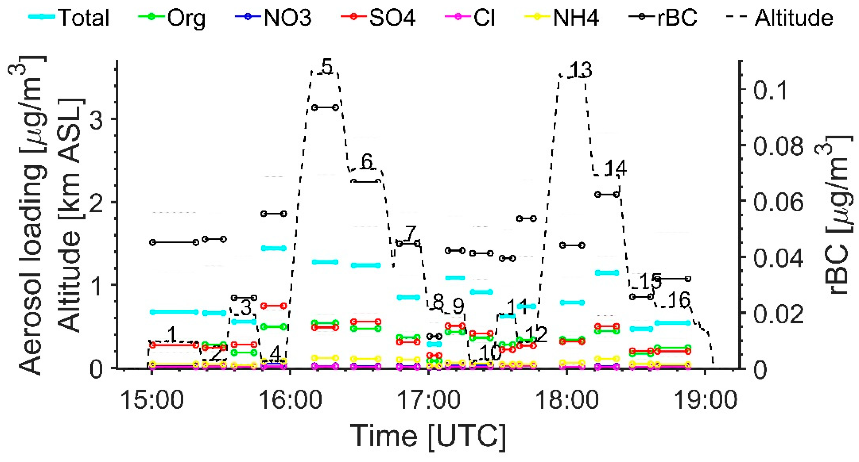
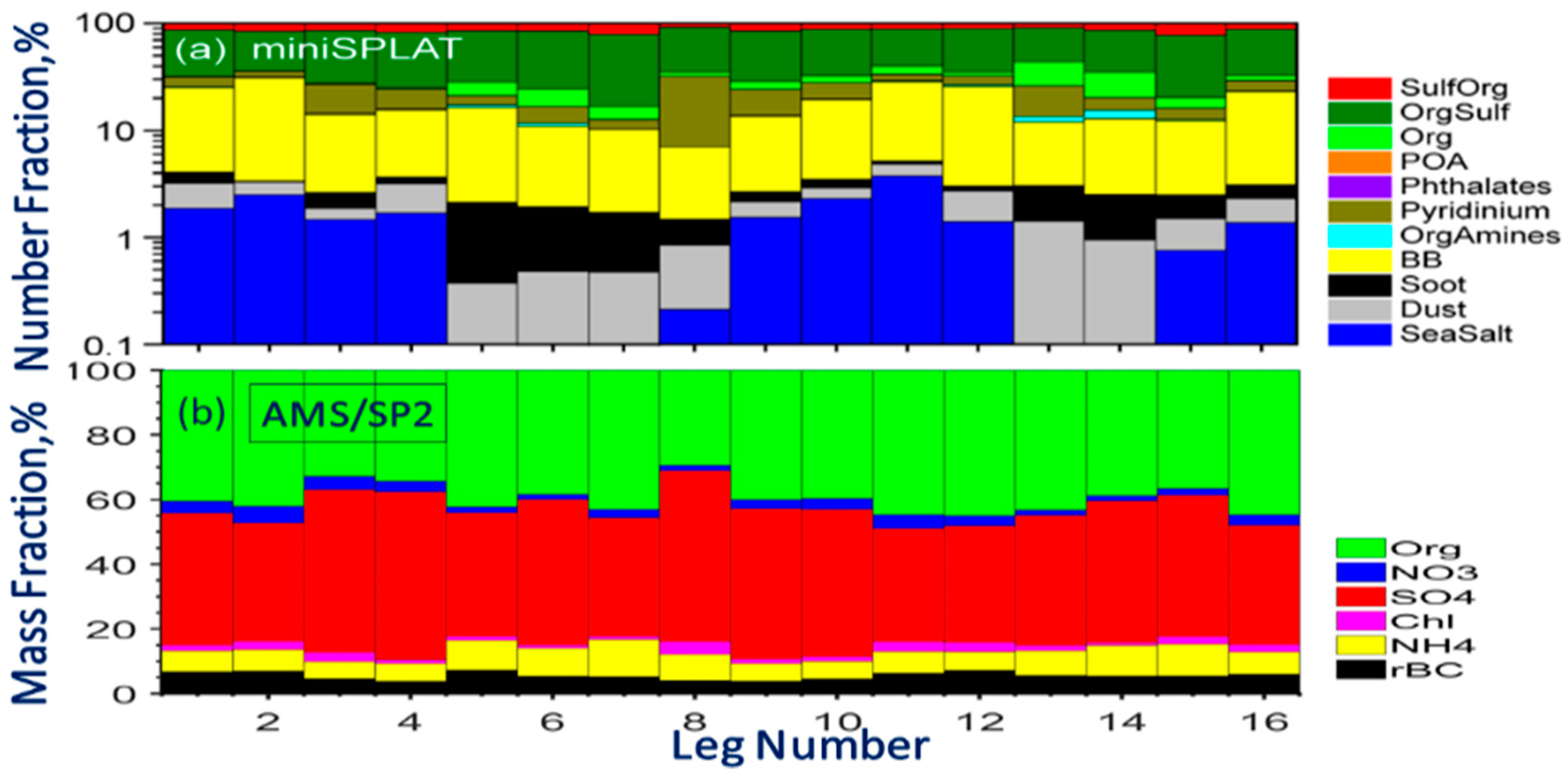
2. Data
3. Model and Adjustments
3.1. Hygroscopic Growth Factor
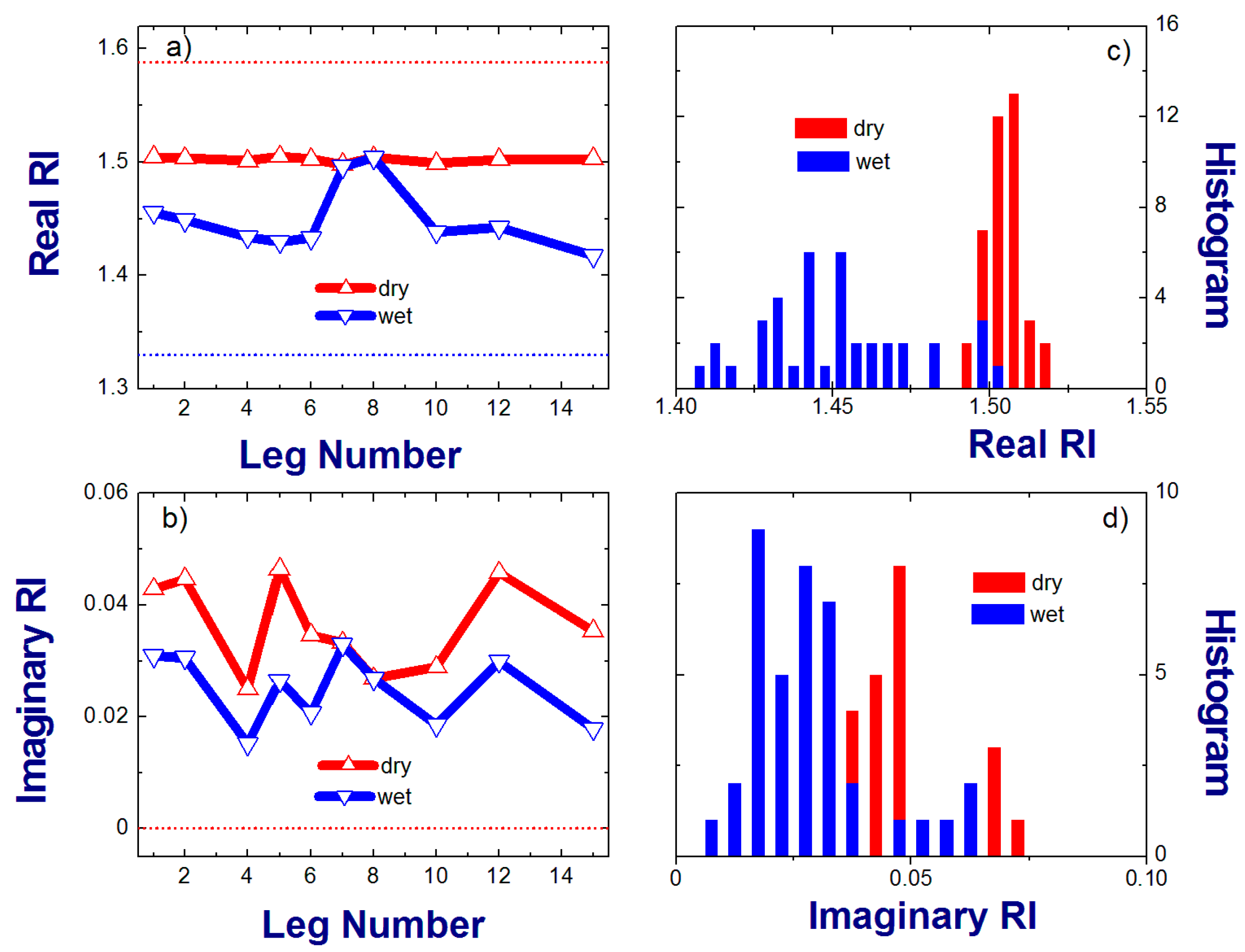
3.2. Dry and Wet Refractive Indices
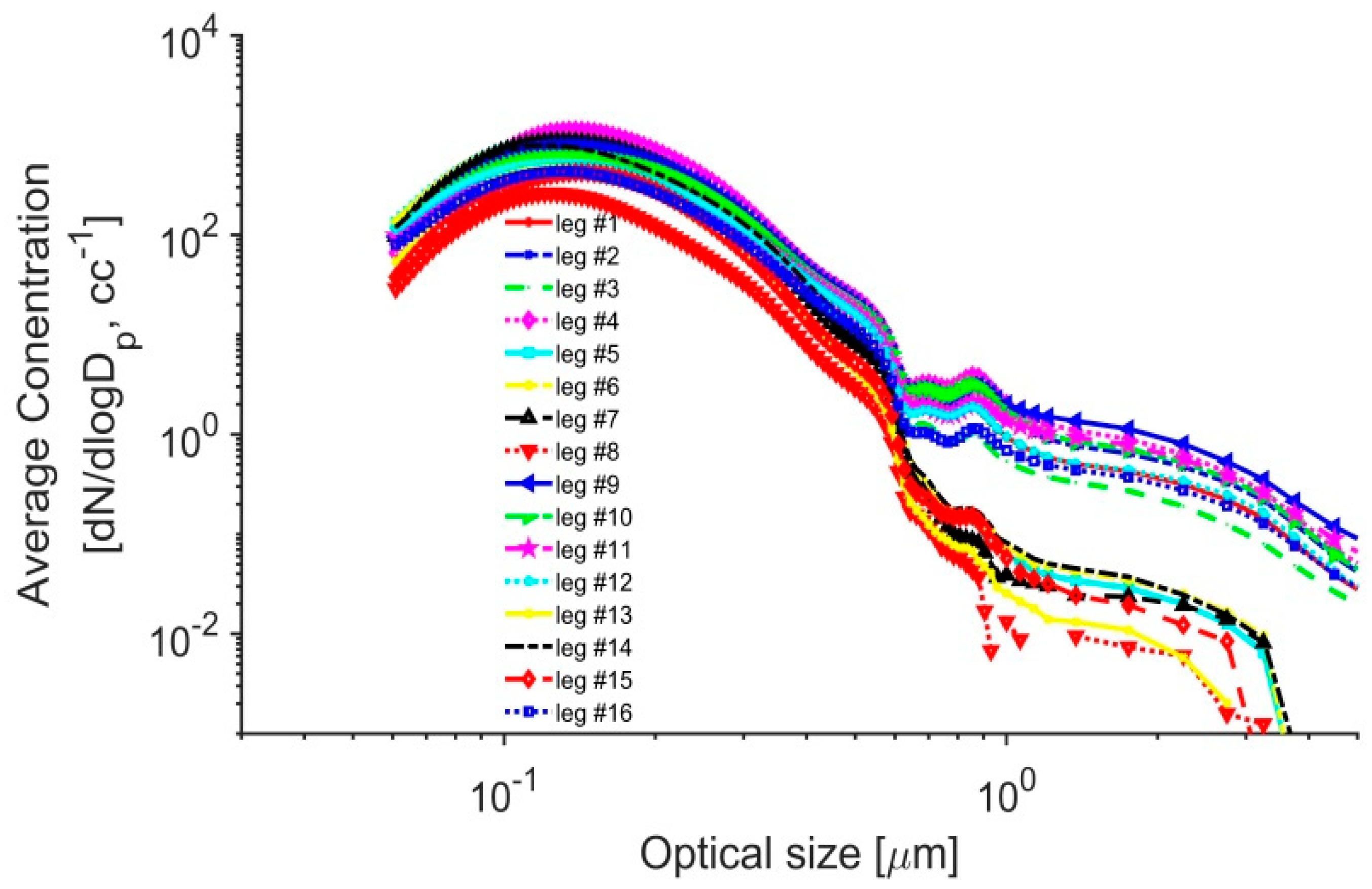
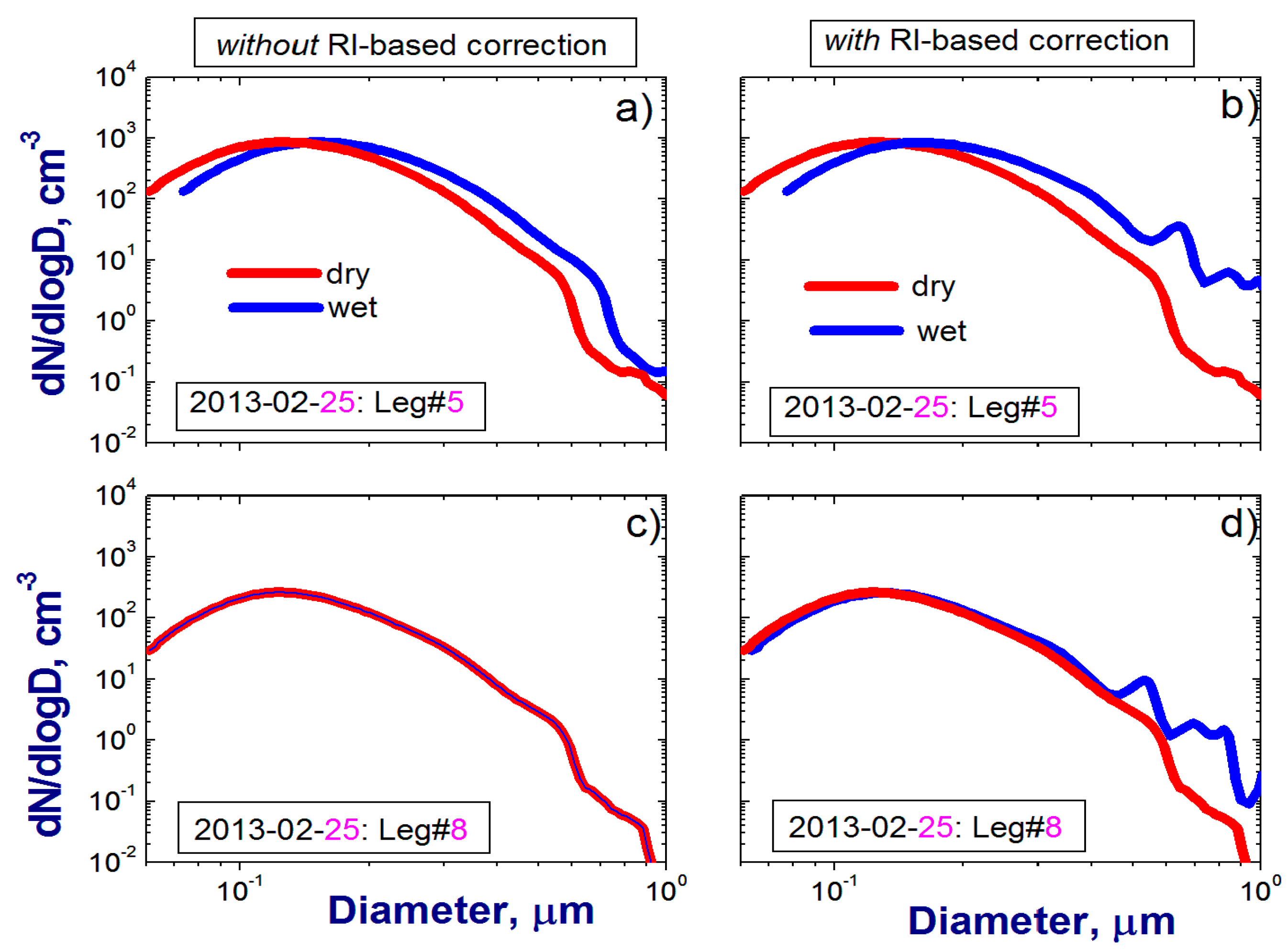
3.3. Size Distribution
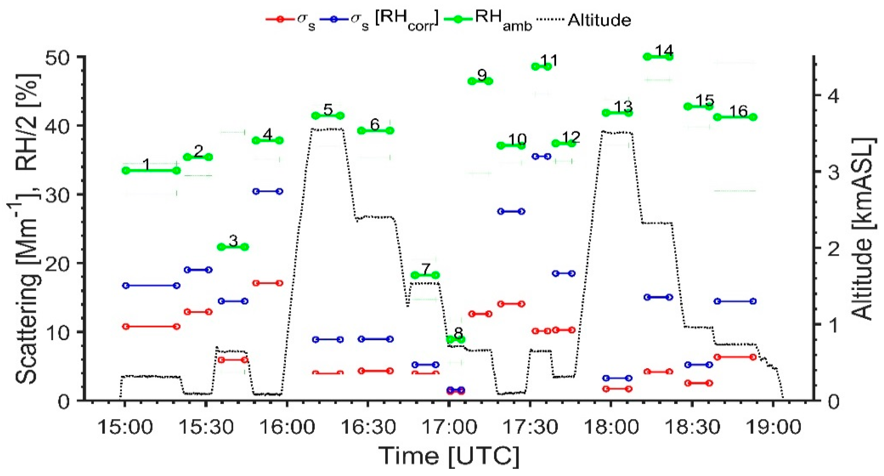
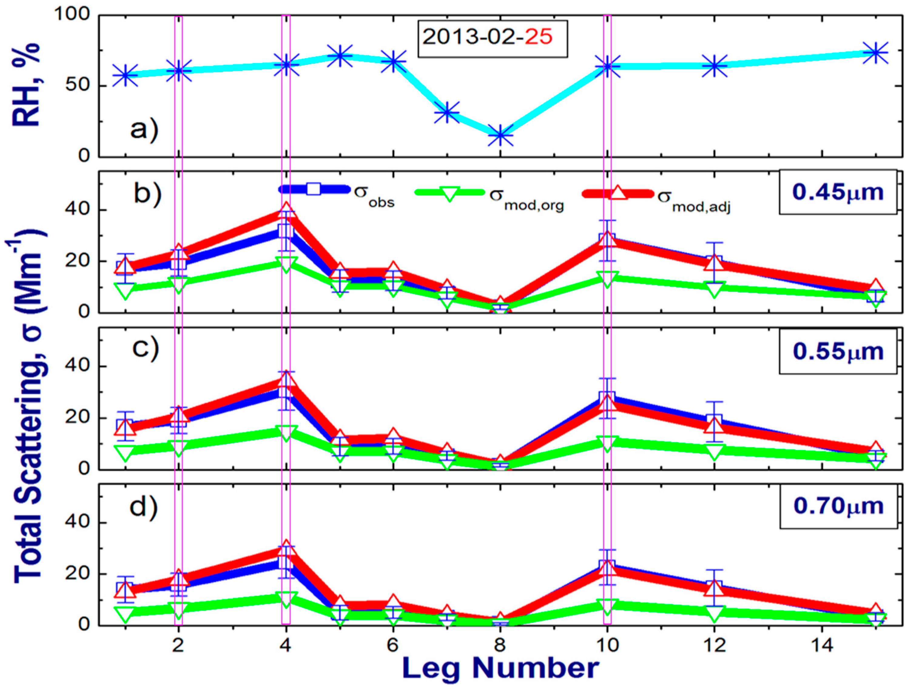
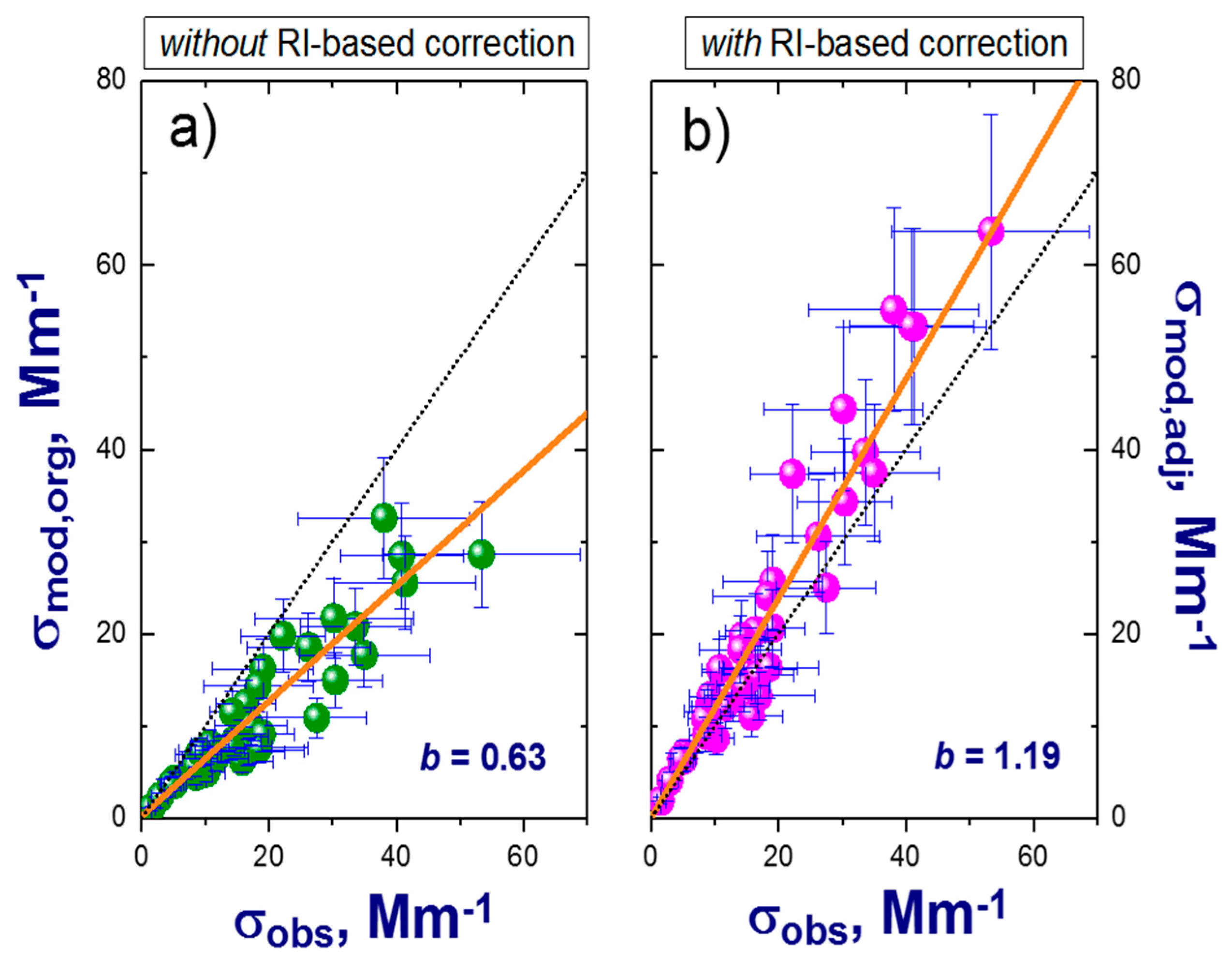
3.4. Scattering Coefficient Calculations
4. Results and Discussion
5. Summary
Author Contributions
Funding
Conflicts of Interest
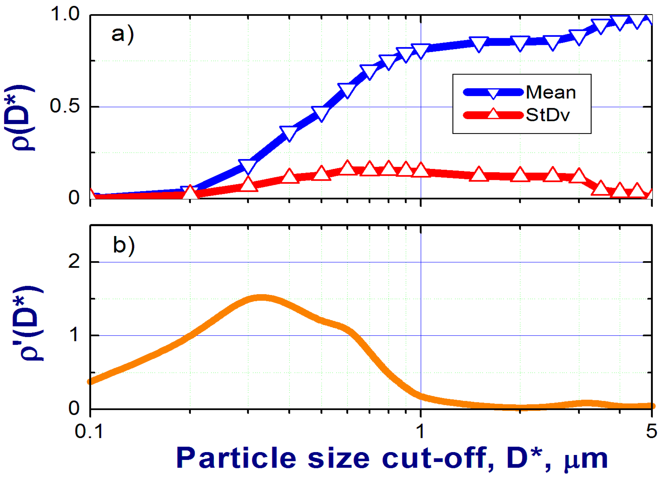
Appendix A. Contributions from Particles of Different Sizes to Scattering

References
- Esteve, A.R.; Highwood, E.J.; Ryder, C.L. A case study of the radiative effect of aerosols over Europe: EUCAARI-LONGREX. Atmos. Chem. Phys. 2016, 16, 7639–7651. [Google Scholar] [CrossRef]
- Lacagnina, C.; Hasekamp, O.P.; Torres, O. Direct radiative effect of aerosols based on PARASOL and OMI satellite observations. J. Geophys. Res. 2017, 122, 2366–2388. [Google Scholar] [CrossRef]
- Hand, J.L.; Gill, T.E.; Schichtel, B.A. Spatial and seasonal variability in fine mineral dust and coarse aerosol mass at remote sites across the United States. J. Geophys. Res. 2017, 122, 3080–3097. [Google Scholar] [CrossRef]
- Hallar, A.G.; Molotch, N.P.; Hand, J.L.; Livneh, B.; McCubbin, I.B.; Petersen, R.; Michalsky, J.; Lowenthal, D.; Kunkel, K.E. Impacts of increasing aridity and wildfires on aerosol loading in the intermountain western US. Environ. Res. Lett. 2017, 12. [Google Scholar] [CrossRef]
- Fast, J.D.; Gustafson, W.I., Jr.; Easter, R.C.; Zaveri, R.A.; Barnard, J.C.; Chapman, E.G.; Grell, G.A.; Peckham, S.E. Evolution of ozone, particulates, and aerosol direct radiative forcing in the vicinity of Houston using a fully coupled meteorology-chemistry-aerosol model. J. Geophys. Res. 2006, 111, D21305. [Google Scholar] [CrossRef]
- Fiedler, S.; Stevens, B.; Mauritsen, T. On the sensitivity of anthropogenic aerosol forcing to model-internal variability and parameterizing a Twomey effect. J. Adv. Model. Earth Syst. 2017, 9, 1325–1341. [Google Scholar] [CrossRef] [Green Version]
- Eck, T.F.; Holben, B.N.; Reid, J.S.; Sinyuk, A.; Dubovik, O.; Smirnov, A.; Giles, D.; O’Neill, N.T.; Tsay, S.C.; Ji, Q.; et al. Spatial and temporal variability of column-integrated aerosol optical properties in the southern Arabian Gulf and United Arab Emirates in summer. J. Geophys. Res. 2008, 113, D01204. [Google Scholar] [CrossRef]
- Titos, G.; Jefferson, A.; Sheridan, P.J.; Andrews, E.; Lyamani, H.; Alados-Arboledas, L.; Ogren, J.A. Aerosol light-scattering enhancement due to water uptake during TCAP campaign. Atmos. Chem. Phys. 2014, 14, 7031–7043. [Google Scholar] [CrossRef]
- Kassianov, E.I.; Barnard, J.C.; Pekour, M.S.; Berg, L.K.; Michalsky, J.J.; Lantz, K.; Hodges, G.B. Do Diurnal Aerosol Changes Affect Daily Average Radiative Forcing? Geophys. Res. Lett. 2013, 40, 3265–3269. [Google Scholar] [CrossRef]
- Berg, L.K.; Fast, J.D.; Barnard, J.C.; Burton, S.P.; Cairns, B.; Chand, D.; Comstock, J.M.; Dunagan, S.; Ferrare, R.A.; Flynn, C.J.; et al. The Two-Column Aerosol Project: Phase I—Overview and Impact of Elevated Aerosol Layers on Aerosol Optical Depth. J. Geophys. Res. 2016, 121, 336–361. [Google Scholar] [CrossRef]
- Berg, L.K.; Fast, J.D.; Barnard, J.C.; Chand, D.; Comstock, J.M.; Pekour, M.; Sedlacek, A.J.; Shilling, J.E.; Tomlinson, J.M.; Zelenyuk, A.; et al. The Two-Column Aerosol Project: Phase II. J. Geophys. Res. 2018. in preparation. [Google Scholar]
- Schuster, G.L.; Dubovik, O.; Holben, B.N. Angstrom exponent and bimodal aerosol size distributions. J. Geophys. Res. 2006, 111, D07207. [Google Scholar] [CrossRef]
- Schmid, B.; Tomlinson, J.M.; Hubbe, J.M.; Comstock, J.M.; Mei, F.; Chand, D.; Pekour, M.S.; Kluzek, C.D.; Andrews, E.; Biraud, S.C.; et al. The DOE ARM Aerial Facility. Bull. Am. Meteor. Soc. 2014, 95, 723–742. [Google Scholar] [CrossRef]
- Babu, S.S.; Nair, V.S.; Gogoi, M.M.; Moorthy, K.K. Seasonal variation of vertical distribution of aerosol single scattering albedo over Indian sub-continent: RAWEX aircraft observations. Atmos. Environ. 2016, 125, 312–323. [Google Scholar] [CrossRef]
- Russell, P.B.; Kinne, S.A.; Bergstrom, R.W. Aerosol climate effects: Local radiative forcing and column closure experiments. J. Geophys. Res. 1997, 102, 9397–9407. [Google Scholar] [CrossRef] [Green Version]
- Schmid, B.; Livingston, J.M.; Russell, P.B.; Durkee, P.A.; Jonsson, H.H.; Collins, D.R.; Flagan, R.C.; Seinfeld, J.H.; Gassó, S.; Hegg, D.A.; et al. Clear-sky closure studies of lower tropospheric aerosol and water vapor during ACE-2 using airborne sunphotometer, airborne in-situ, space-borne, and ground-based measurements. Tellus B 2000, 52, 568–593. [Google Scholar] [CrossRef]
- Malm, W.C.; Day, D.E.; Carrico, C.; Kreidenweis, S.M.; Collett, J.L., Jr.; McMeeking, G.; Lee, T.; Carrillo, J.; Schichtel, B. Intercomparison and closure calculations using measurements of aerosol species and optical properties during the Yosemite Aerosol Characterization Study. J. Geophys. Res. 2005, 110, D14302. [Google Scholar] [CrossRef]
- Mack, L.A.; Levin, E.J.T.; Kreidenweis, S.M.; Obrist, D.; Moosmüller, H.; Lewis, K.A.; Arnott, W.P.; McMeeking, G.R.; Sullivan, A.P.; Wold, C.E.; et al. Optical closure experiments for biomass smoke aerosols. Atmos. Chem. Phys. 2010, 10, 9017–9026. [Google Scholar] [CrossRef] [Green Version]
- Kassianov, E.; Berg, L.K.; Pekour, M.; Barnard, J.; Chand, D.; Flynn, C.; Ovchinnikov, M.; Sedlacek, A.; Schmid, B.; Shilling, J.; et al. Airborne Aerosol in Situ Measurements during TCAP: A Closure Study of Total Scattering. Atmosphere 2015, 6, 1069–1101. [Google Scholar] [CrossRef] [Green Version]
- Allen, G.; Coe, H.; Clarke, A.; Bretherton, C.; Wood, R.; Abel, S.J.; Barrett, P.; Brown, P.; George, R.; Freitag, S.; et al. South East Pacific atmospheric composition and variability sampled along 20° S during VOCALS-Rex. Atmos. Chem. Phys. 2011, 11, 5237–5262. [Google Scholar] [CrossRef] [Green Version]
- Kleinman, L.I.; Daum, P.H.; Lee, Y.-N.; Lewis, E.R.; Sedlacek, A.J., III; Senum, G.I.; Springston, S.R.; Wang, J.; Hubbe, J.; Jayne, J.; et al. Aerosol concentration and size distribution measured below, in, and above cloud from the DOE G-1 during VOCALS-REx. Atmos. Chem. Phys. 2012, 11, 207–223. [Google Scholar] [CrossRef]
- Markowski, G.R. Improving Twomey’s Algorithm for Inversion of Aerosol Measurement Data. Aerosol Sci. Technol. 1987, 7, 127–141. [Google Scholar] [CrossRef]
- Collins, D.R.; Flagan, R.C.; Seinfeld, J.H. Improved inversion of scanning DMA data. Aerosol Sci. Technol. 2002, 36, 1–9. [Google Scholar] [CrossRef]
- Jayne, J.T.; Leard, D.C.; Zhang, X.F.; Davidovits, P.; Smith, K.A.; Kolb, C.E.; Worsnop, D.R. Development of an aerosol mass spectrometer for size and composition analysis of submicron particles. Aerosol Sci. Technol. 2000, 33, 49–70. [Google Scholar] [CrossRef]
- DeCarlo, P.F.; Kimmel, J.R.; Trimborn, A.; Northway, M.J.; Jayne, J.T.; Aiken, A.C.; Gonin, M.; Fuhrer, K.; Horvath, T.; Docherty, K.S.; et al. Field-deployable, high-resolution, time-of-flight aerosol mass spectrometer. Anal. Chem. 2006, 78, 8281–8289. [Google Scholar] [CrossRef] [PubMed]
- Moteki, N.; Kondo, Y. Effects of mixing state on black carbon measurements by laser-induced incandescence. Aerosol Sci. Technol. 2007, 41, 398–417. [Google Scholar] [CrossRef]
- Sedlacek, A.J., III; Lewis, E.R.; Kleinman, L.; Xu, J.; Zhang, Q. Determination of and evidence for non-core-shell structure of particles containing black carbon using the Single-Particle Soot Photometer (SP2). Geophys. Res. Lett. 2012, 39. [Google Scholar] [CrossRef] [Green Version]
- Liu, P.; Ziemann, P.J.; Kittelson, D.B.; McMurry, P.H. Generating Particle Beams of Controlled Dimensions and Divergence: I. Theory of Particle Motion in Aerodynamic Lenses and Nozzle Expansions. Aerosol Sci. Technol. 1995, 22, 293–313. [Google Scholar] [CrossRef] [Green Version]
- Zelenyuk, A.; Imre, D.; Wilson, J.; Zhang, Z.; Wang, J.; Mueller, K. Airborne Single Particle Mass Spectrometers (SPLAT II & miniSPLAT) and new software for data visualization and analysis in a geo-spatial context. J. Am. Soc. Mass Spectrom. 2015, 26, 257–270. [Google Scholar] [PubMed]
- Vaden, T.D.; Imre, D.; Beranek, J.; Zelenyuk, A. Extending the capabilities of single particle mass spectrometry: II. Measurements of aerosol particle density without DMA. Aerosol Sci. Technol. 2011, 45, 125–135. [Google Scholar] [CrossRef]
- Pekour, M.S.; Schmid, B.; Chand, D.; Hubbe, J.M.; Kluzek, C.D.; Nelson, D.A.; Tomlinson, J.M.; Cziczo, D.J. Development of a new airborne humidigraph system. Aerosol Sci. Technol. 2013, 47, 201–207. [Google Scholar] [CrossRef]
- Shinozuka, Y.; Johnson, R.R.; Flynn, C.J.; Russell, P.B.; Schmid, B.; Redemann, J.; Dunagan, S.E.; Kluzek, C.D.; Hubbe, J.M.; Segal-Rosenheimer, M.; et al. Hyperspectral aerosol optical depths from TCAP flights. J. Geophys. Res. Atmos. 2013, 118, 12180–12194. [Google Scholar] [CrossRef]
- Anderson, T.L.; Ogren, J.A. Determining aerosol radiative properties using the TSI 3563 Integrating Nephelometer. Aerosol Sci. Technol. 1998, 29, 57–69. [Google Scholar] [CrossRef]
- Hallar, A.G.; Strawa, A.W.; Schmid, B.; Andrews, E.; Ogren, J.; Sheridan, P.; Ferrare, R.; Covert, D.; Elleman, R.; Jonsson, H.; et al. Atmospheric Radiation Measurements Aerosol Intensive Operating Period: Comparison of aerosol scattering during coordinated flights. J. Geophys. Res. 2006, 111, D05S09. [Google Scholar] [CrossRef]
- Weber, R.J.; Clarke, A.D.; Litchy, M.; Li, J.; Kok, G.; Schillawski, R.D.; McMurry, P.H. Spurious aerosol measurements when sampling from aircraft in the vicinity of clouds. J. Geophys. Res. 1998, 103, 28337–28346. [Google Scholar] [CrossRef] [Green Version]
- Smirnov, A.; Sayer, A.M.; Holben, B.N.; Hsu, N.C.; Sakerin, S.M.; Macke, A.; Nelson, N.B.; Courcoux, Y.; Smyth, T.J.; Croot, P.; et al. Effect of wind speed on aerosol optical depth over remote oceans, based on data from the Maritime Aerosol Network. Atmos. Meas. Tech. 2012, 5, 377–388. [Google Scholar] [CrossRef] [Green Version]
- Particle-into-Liquid Sampler Instrument Handbook. Available online: https://www.arm.gov/publications/tech_reports/handbooks/pils_handbook.pdf (accessed on 11 June 2018).
- Seinfeld, J.H.; Pandis, S.N. Atmospheric Chemistry and Physics: From Air Pollution to Climate Change; John Wiley and Sons Ltd.: Hoboken, NJ, USA, 2016. [Google Scholar]
- Esteve, A.R.; Highwood, E.J.; Morgan, W.T.; Allen, G.; Coe, H.; Grainger, R.G.; Brown, P.; Szpek, K. A study on the sensitivities of simulated aerosol optical properties to composition and size distribution using airborne measurements. Atmos. Environ. 2014, 89, 517–524. [Google Scholar] [CrossRef]
- Hu, D.; Chen, J.; Ye, X.; Li, L.; Yang, X. Hygroscopicity and evaporation of ammonium chloride and ammonium nitrate: Relative humidity and size effects on the growth factor. Atmos. Environ. 2011, 45, 2349–2355. [Google Scholar] [CrossRef]
- Healy, R.M.; Evans, G.J.; Murphy, M.; Jurányi, Z.; Tritscher, T.; Laborde, M.; Weingartner, E.; Gysel, M.; Poulain, L.; Kamilli, K.A.; et al. Predicting hygroscopic growth using single particle chemical composition estimates. J. Geophys. Res. Atmos. 2014, 119, 9567–9577. [Google Scholar] [CrossRef] [Green Version]
- Xie, Y.S.; Li, Z.Q.; Zhang, Y.X.; Zhang, Y.; Li, D.H.; Li, K.T.; Xu, H.; Wang, Y.Q.; Chen, X.F.; Schauer, J.J.; Bergin, M. Estimation of atmospheric aerosol composition from ground-based remote sensing measurements of Sun-sky radiometer. J. Geophys. Res. Atmos. 2017, 122, 498–518. [Google Scholar] [CrossRef]
- Marshall, J.; Lohmann, U.; Leaitch, W.R.; Lehr, P.; Hayden, K. Aerosol scattering as a function of altitude in a coastal environment. J. Geophys. Res. 2007, 112, D14203. [Google Scholar] [CrossRef]
- Zieger, P.; Fierz-Schmidhauser, R.; Poulain, L.; Müller, T.; Birmili, W.; Spindler, G.; Wiedensohler, A.; Baltensperger, U.; Weingartner, E. Influence of water uptake on the aerosol particle light scattering coefficients of the Central European aerosol. Tellus B 2014, 66, 22716. [Google Scholar] [CrossRef] [Green Version]
- Barnard, J.C.; Fast, J.D.; Paredes-Miranda, G.; Arnott, W.P.; Laskin, A. Technical note: Evaluation of the WRF-Chem “Aerosol chemical to aerosol optical properties” module using data from the MILAGRO campaign. Atmos. Chem. Phys. 2010, 10, 7325–7340. [Google Scholar] [CrossRef]
- Pilinis, C.; Charalampidis, P.E.; Mihalopoulos, N.; Pandis, S.N. Contribution of particulate water to the measured aerosol optical properties of aged aerosol. Atmos. Environ. 2014, 82, 144–153. [Google Scholar] [CrossRef]
- Wex, H.; Neususs, C.; Wendisch, M.; Stratmann, F.; Koziar, C.; Keil, A.; Wiedensohler, A.; Ebert, M. Particle scattering, backscattering, and absorption coefficients: An in situ closure and sensitivity study. J. Geophys. Res. Atmos. 2012, 107, 8122. [Google Scholar] [CrossRef]
- York, D.; Evensen, N.M.; Lopez Martinez, M.; de Basabe Delgado, J. Unified equations for the slope, intercept, and standard errors of the best straight line. Am. J. Phys. 2004, 72, 367–375. [Google Scholar] [CrossRef]
- Zelenyuk, A.; Imre, D.; Han, J.H.; Oatis, S. Simultaneous measurements of individual ambient particle size, composition, effective density, and hygroscopicity. Anal. Chem. 2008, 80, 1401–1407. [Google Scholar] [CrossRef] [PubMed]
- Zelenyuk, A.; Imre, D.; Earle, M.; Easter, R.; Korolev, A.; Leaitch, R.; Liu, P.; Macdonald, A.M.; Ovchinnikov, M.; Strapp, W. In Situ Characterization of Cloud Condensation Nuclei, Interstitial, and Background Particles Using the Single Particle Mass Spectrometer, SPLAT II. Anal. Chem. 2010, 82, 7943–7951. [Google Scholar] [CrossRef] [PubMed]
- Friedman, B.; Zelenyuk, A.; Beranek, J.; Kulkarni, G.; Pekour, M.; Gannet Hallar, A.; McCubbin, I.B.; Thornton, J.A.; Cziczo, D.J. Aerosol measurements at a high-elevation site: Composition, size, and cloud condensation nuclei activity. Atmos. Chem. Phys. 2013, 13, 11839–11851. [Google Scholar] [CrossRef]
- Seinfeld, J.H.; Bretherton, C.; Carslaw, K.S.; Coe, H.; DeMott, P.J.; Dunlea, E.J.; Feingold, G.; Ghan, S.; Guenther, A.B.; Kahn, R.; et al. Improving our fundamental understanding of the role of aerosol−cloud interactions in the climate system. Proc. Natl. Acad. Sci. USA 2016, 113, 5781–5790. [Google Scholar] [CrossRef] [PubMed] [Green Version]
- Shinozuka, Y.; Redemann, J.; Livingston, J.M.; Russell, P.B.; Clarke, A.D.; Howell, S.G.; Freitag, S.; O’Neill, N.T.; Reid, E.A.; Johnson, R.; et al. Airborne observation of aerosol optical depth during ARCTAS: Vertical profiles, inter-comparison and fine-mode fraction. Atmos. Chem. Phys. 2011, 11, 3673–3688. [Google Scholar] [CrossRef] [Green Version]
- Ching, J.; Fast, J.D.; West, M.; Riemer, N.R. Metrics to quantify the importance of mixing state for CCN activity. Atmos. Chem. Phys. 2017, 17, 7445–7458. [Google Scholar] [CrossRef] [Green Version]
- Ching, J.; Zaveri, R.A.; Easter, R.C.; Riemer, N.; Fast, J.D. A three-dimensional sectional representation of aerosol mixing state for simulating optical properties and cloud condensation nuclei. J. Geophys. Res. 2016, 121, 5912–5929. [Google Scholar] [CrossRef]


| Parameters | OM | SO4 | NO3 | Cl | NH4 | rBC | Water | NaCl |
|---|---|---|---|---|---|---|---|---|
| Density (g/cm3) | 1.4 | 1.8 | 1.8 | 1.53 | 1.8 | 1.8 | 1.0 | 2.2 |
| RI (real) | 1.45 | 1.52 | 1.5 | 1.64 | 1.5 | 1.85 | 1.33 | 1.55 |
| RI (imag) | 0.0 | 0 | 0 | 0 | 0 | 0.71 | 0 | 0 |
| HGF (RH = 80%) | 1.07 | 1.50 | 1.50 | 1.9 | 1.50 | 1.0 | - | 1.9 |
| Scattering Coefficients | Mean | StDv | RMSE | a | b |
|---|---|---|---|---|---|
| 0.45 µm | |||||
| σobs | 21.80 | 14.35 | - | - | - |
| σmod,org | 15.96 | 11.04 | 7.51 | 0.30 (0.60) | 0.73 (0.06) |
| σmod,adj | 26.73 | 18.86 | 7.56 | 0.11 (0.99) | 1.22 (0.10) |
| 0.55 µm | |||||
| σobs | 18.18 | 12.11 | - | - | - |
| σmod,org | 11.39 | 7.94 | 8.77 | 0.21 (0.42) | 0.63 (0.05) |
| σmod,adj | 21.68 | 15.72 | 6.17 | 0.08 (0.79) | 1.19 (0.10) |
| 0.70 µm | |||||
| σobs | 12.89 | 9.17 | - | - | - |
| σmod,org | 7.34 | 5.28 | 7.43 | 0.23 (0.26) | 0.56 (0.05) |
| σmod,adj | 16.43 | 12.77 | 6.07 | 0.25 (0.57) | 1.25 (0.11) |
© 2018 by the authors. Licensee MDPI, Basel, Switzerland. This article is an open access article distributed under the terms and conditions of the Creative Commons Attribution (CC BY) license (http://creativecommons.org/licenses/by/4.0/).
Share and Cite
Kassianov, E.; Berg, L.K.; Pekour, M.; Barnard, J.; Chand, D.; Comstock, J.; Flynn, C.; Sedlacek, A.; Shilling, J.; Telg, H.; et al. A Closure Study of Total Scattering Using Airborne In Situ Measurements from the Winter Phase of TCAP. Atmosphere 2018, 9, 228. https://doi.org/10.3390/atmos9060228
Kassianov E, Berg LK, Pekour M, Barnard J, Chand D, Comstock J, Flynn C, Sedlacek A, Shilling J, Telg H, et al. A Closure Study of Total Scattering Using Airborne In Situ Measurements from the Winter Phase of TCAP. Atmosphere. 2018; 9(6):228. https://doi.org/10.3390/atmos9060228
Chicago/Turabian StyleKassianov, Evgueni, Larry K. Berg, Mikhail Pekour, James Barnard, Duli Chand, Jennifer Comstock, Connor Flynn, Arthur Sedlacek, John Shilling, Hagen Telg, and et al. 2018. "A Closure Study of Total Scattering Using Airborne In Situ Measurements from the Winter Phase of TCAP" Atmosphere 9, no. 6: 228. https://doi.org/10.3390/atmos9060228