Machine Learning Models Coupled with Variational Mode Decomposition: A New Approach for Modeling Daily Rainfall-Runoff


1
Department of Constructional and Environmental Engineering, Kyungpook National University, Sangju 37224, Korea
2
Department of Railroad Construction and Safety Engineering, Dongyang University, Yeongju 36040, Korea
3
Department of Biological and Agricultural Engineering & Zachry Department of Civil Engineering, Texas A & M University, College Station, TX 77843-2117, USA
*
Author to whom correspondence should be addressed.
Atmosphere 2018, 9(7), 251; https://doi.org/10.3390/atmos9070251
Submission received: 24 May 2018
/
Revised: 2 July 2018
/
Accepted: 3 July 2018
/
Published: 5 July 2018
(This article belongs to the Special Issue Integration of Advanced Soft Computing Techniques in Hydrological Predictions)
Abstract
:Accurate modeling for nonlinear and nonstationary rainfall-runoff processes is essential for performing hydrologic practices effectively. This paper proposes two hybrid machine learning models (MLMs) coupled with variational mode decomposition (VMD) to enhance the accuracy for daily rainfall-runoff modeling. These hybrid MLMs consist of VMD-based extreme learning machine (VMD-ELM) and VMD-based least squares support vector regression (VMD-LSSVR). The VMD is employed to decompose original input and target time series into sub-time series called intrinsic mode functions (IMFs). The ELM and LSSVR models are selected for developing daily rainfall-runoff models utilizing the IMFs as inputs. The performances of VMD-ELM and VMD-LSSVR models are evaluated utilizing efficiency and effectiveness indices. Their performances are also compared with those of VMD-based artificial neural network (VMD-ANN), discrete wavelet transform (DWT)-based MLMs (DWT-ELM, DWT-LSSVR, and DWT-ANN) and single MLMs (ELM, LSSVR, and ANN). As a result, the VMD-based MLMs provide better accuracy compared with the single MLMs and yield slightly better performance than the DWT-based MLMs. Among all models, the VMD-ELM and VMD-LSSVR models achieve the best performance in daily rainfall-runoff modeling with respect to efficiency and effectiveness. Therefore, the VMD-ELM and VMD-LSSVR models can be an alternative tool for reliable and accurate daily rainfall-runoff modeling.
1. Introduction
Estimating rainfall-runoff relationship and streamflow accurately is a significant element which should be considered for managing water resources effectively [1,2]. Hydrologic practices, including water supply and allocation, reservoir planning and operation, flood and drought management, and other hydrological applications, can be conducted successfully only when the rainfall-runoff relationship and streamflow behavior in a river watershed are estimated accurately. However, the development of accurate rainfall-runoff and streamflow models is still a challenging task since hydrological processes inherently exhibit nonlinear and complex behavior [3].
According to Wang [4], rainfall-runoff and streamflow models can be largely categorized into process-driven models (also known as white-box, physical or conceptual models) and data-driven models (also called black-box, meta-models or surrogate models). The process-driven models are based on the physical interpretation of watershed system. These models are formulated utilizing complex physical equations and parametric assumptions [2]. Contrastively, the data-driven models characterize the relationship between input and output, not describing the natural watershed process [2,5]. The modeling simplicity and high accuracy have increased hydrologists’ attention for rainfall-runoff and streamflow modeling based on the data-driven models. Furthermore, the increased availability of gauging data, the development of advanced modeling techniques, and the increase of computing power have accelerated the development of rainfall-runoff and streamflow models utilizing the data-driven models [2].
Over the last few decades, the development of data-driven rainfall-runoff and streamflow models has been conducted using statistical time series models (also called stochastic models), including autoregressive (AR), autoregressive moving average (ARMA), autoregressive integrated moving average (ARIMA), and transfer function-noise (TFN) models [5,6]. Since rainfall-runoff relationship and streamflow time series are usually highly non-stationary and nonlinear, it has been noted that the modeling capability of these models classified as linear models is limited [5,7].
To overcome the limitation of the statistical time series models, various machine learning models (MLMs) have been applied successfully for rainfall-runoff and streamflow modeling. The MLMs included artificial neural network (ANN) [1,8], neuro-fuzzy (NF) [9], support vector machines (SVMs) (for regression, also called support vector regression (SVR)) [10,11], random forest (RF) [12], least squares support vector machine (LSSVM) (for regression, also called least squares support vector regression (LSSVR)) [13,14] and extreme learning machine (ELM) [15,16]. The MLMs are able to deal with nonlinearity and non-stationarity inherent in rainfall-runoff relationship and streamflow time series effectively. Therefore, these models have achieved better performance than the conventional statistical time series models and have been accepted as effective tools for rainfall-runoff and streamflow modeling. The comprehensive review of MLMs can be found in ASCE [17,18], Yassen et al. [19], Fahimi et al. [20], and Fotovatikhah et al. [21].
On the other hand, many studies have also been conducted to enhance the performance of MLMs for rainfall-runoff and streamflow modeling. These studies were mostly on the development of hybrid MLMs in which the MLMs were combined with various statistical and mathematical methods. The hybrid model development for rainfall-runoff and streamflow modeling can be classified into the following four types. First, to improve the model performance, the MLMs have been combined with statistical methods, including phase-space reconstruction [22,23], principal component analysis [24,25], fuzzy c-means clustering [7,22], k-means clustering [26,27], self-organizing map (SOM) [28,29] and bootstrap [30]. Second, the MLMs have been coupled with evolutionary optimization algorithms, including genetic algorithm (GA) [31,32], particle swarm optimization (PSO) [11,33], artificial bee colony [34], bat algorithm [35], and firefly algorithm [36]. The addressed algorithms were very helpful for efficient model learning and optimal parameter searching. Third, as the preprocessing techniques of the MLMs, time series decomposition methods have been applied to hybrid MLMs development. The methods included discrete wavelet transform (DWT) [37,38], maximal overlap DWT (MODWT) [39], wavelet packet transform (WPT) [40], empirical mode decomposition (EMD) [41,42], and ensemble EMD (EEMD) [43,44]. It has been reported that these hybrid MLMs, which consists of time series decomposition and sub-time series modeling, were able to achieve better performance compared with the single MLMs. Finally, the hybrid MLMs, combined with more than two methods, have been developed for rainfall-runoff and streamflow modeling including DWT, PSO, and SVMs [45]; DWT, GA, and adaptive neuro-fuzzy inference system (ANFIS) [46]; EEMD, PSO, and SVMs [47]; EEMD, SOM, and linear genetic programming [48]; wavelet transform, singular spectrum, chaotic approach, and SVR [49]; and Hermite-projection pursuit regression, social spider optimization, and least square algorithm [50].
Especially, the time series decomposition methods, including DWT, MODWT, WPT, EMD, and EEMD, have been effectively applied for improving the performance of MLMs in rainfall-runoff and streamflow modeling. Using the addressed methods, an original time series was decomposed into sub-time series, and the MLMs were then modeled utilizing the decomposed sub-time series. Using the detailed expressions, the DWT and MODWT, which are data-preprocessing techniques for analyzing a time series in time-frequency domains, produce a low-frequency component (approximation) and multiple high-frequency components (details) by decomposing an original time series, whereas the WPT decomposes both the approximation and the details at each level. It has been reported that these wavelet transform methods were effective tools for improving the performance of MLMs in rainfall-runoff and streamflow modeling since the methods were able to capture the useful information in different levels [51]. Adamowski and Sun [39] presented an ANN model combined with MODWT for daily streamflow forecasting and confirmed that the hybrid model produced the better accuracy than the single ANN model for daily streamflow. Kisi and Cimen [37] examined the accuracy of a hybrid model combining DWT and SVMs to predict monthly streamflow and suggested that the conjunction model could enhance the prediction accuracy of SVMs. Liu et al. [38] developed the conjunction model of DWT and SVR for forecasting daily and monthly streamflow and investigated the performance of conjunction model. They considered the wavelet decomposition factors, including decomposition level, mother wavelet and edge effect, for improving the model accuracy. They found that the ensemble approach was able to produce better performance compared with the best single DWT-SVR model. Zhang et al. [45] developed a streamflow forecasting model combining SVM with wavelet transform (WT) and PSO (WT-PSO-SVM). They revealed that the hybrid model provided a better alternative compared with the SVMs for monthly streamflow forecasting. Baydaroğlu et al. [49] presented a coupling model of WT, chaotic approach (CA), singular spectrum analysis (SSA) and SVR. They proved that WT, SSA and CA for configuring the input matrix of the SVR were effective in the hybrid modeling for river flow prediction. Moosavi et al. [40] developed a robust model combining WPT and group method of data handling (GMDH) to estimate daily runoff. He concluded that the WPT dealt with non-stationaries in daily runoff data effectively and improved the performance of GMDH model efficiently.
The EMD and EEMD, which are self-adaptive and empirical methods, generate multiple sub-time series called intrinsic mode functions (IMFs) by decomposing an original time series. The wavelet transform methods work in frequency space and require basis functions (mother wavelets) which should be predetermined, whereas the EMD and EEMD work directly in temporal space and do not require any basis functions [52]. Recently, the hybrid model development utilizing the EMD and EEMD have been applied successfully for rainfall-runoff and streamflow models. Napolitano et al. [41] explored the effects of data preprocessing for EMD-based ANN streamflow model. They found that the advantages of data preprocessing were dependent on the characteristics of intrinsic modes. Wang et al. [47] proposed a coupling of EEMD, PSO and SVMs for forecasting annual rainfall-runoff and concluded that the hybrid approach could improve the accuracy of annual runoff forecasting significantly. Huang et al. [42] assessed the performance of a modified EMD-SVMs model to forecast monthly streamflow and confirmed that the hybrid model provided high prediction accuracy and reliable stability. Wang et al. [43] developed an ANN modeling approach based on EEMD to forecast medium- and long-term runoff. They confirmed that the EEMD was able to increase the forecasting accuracy effectively. Also, the hybrid approach could provide higher forecasting accuracy compared with the single ANN model. Barge and Sharif [48] proposed the coupling of linear genetic programming (LGP), EEMD, and SOM, and they demonstrated the effectiveness of the hybrid model in streamflow forecasting.
Based on the previous studies mentioned above, it can be noted that the time series decomposition techniques, including DWT, MODWT, WPT, EMD, and EEMD, were effective for developing the hybrid MLMs. However, the addressed methods have some drawbacks. As Liu et al. [38] suggested, three factors, namely, decomposition level, mother wavelet and edge effect, should be considered for applying the wavelet methods. Among them, especially, the optimal mother wavelet should be selected through evaluating the performances of the wavelet-based MLMs, depending on different mother wavelets and wavelet indices. Since these factors should be considered for effective wavelet-based MLM modeling, they can make the wavelet-based MLM modeling computationally intensive and time-consuming. The EMD has a disadvantage called the mode mixing [53], which results in incorrect time-frequency representation and consequently degrades the accuracy of time series processing. Furthermore, since the EMD is a recursive algorithm, the error of envelope estimation can be enlarged more and more, and the efficiency can be decreased [54]. The stopping criteria and end-point effect also affect the decomposition process [53]. To alleviate the problems, especially the mode mixing, Wu and Huang [53] proposed the EEMD. Although the problems can be reduced by the EEMD, they did not settle completely. The EEMD still has some unresolved problems including dissatisfaction with requirements for IMF, treatment of multi-mode distribution for IMF, end-point effect, and stopping criteria [53].
Recently, Dragomiretskiy and Zosso [55] developed an adaptive and non-recursive signal analysis technique called the variational mode decomposition (VMD) to resolve the drawback of EMD. Unlike the EMD, the VMD decomposes an original time series into multiple modes and then updates them. As compared to the EMD, the VMD is more robust to sampling and noise, and has excellent performance in frequency search and separation. Furthermore, the VMD can extract the time-frequency features accurately since it can alleviate the mode mixing through yielding narrow-banded modes [54]. Due to these advantages of the VMD, the development of hybrid MLMs based on the VMD has been accomplished successfully in various fields, including renewable energy, financial and economic fields [56,57,58]. On the other hand, the VMD is a relatively new method for hydrological application. Under the authors’ knowledge, the hydrological hybrid MLM modeling based on the VMD has never been attempted. Therefore, the application of the VMD is required for developing hybrid MLMs in hydrological modeling.
Modeling rainfall-runoff relationship accurately is essential for effective hydrologic practices. However, since rainfall-runoff process is nonlinear and nonstationary, accurate rainfall-runoff modeling is very difficult and thus still one of significant tasks in hydrological field. Therefore, this paper proposes hybrid MLMs coupled with VMD for modeling nonlinear and nonstationary rainfall-runoff process effectively. In this study, two hybrid MLMs based on the VMD are proposed including VMD-based ELM (VMD-ELM) and VMD-based LSSVR (VMD-LSSVR). ELM and LSSVR are adopted for developing VMD-based rainfall-runoff models. MLMs including ANN, ANFIS, SVM, RF, etc. can be used as the alternatives. However, ELM and LSSVR have advantages over other models when considering generalization performance, learning speed, over-training, the number of user-defined parameters, and the possibility of getting into local minimum [13,18,59,60,61,62,63,64]. Therefore, in this study, ELM and LSSVR are employed for VMD-based rainfall-runoff modeling and ANN is selected for performance comparison. The model performances are evaluated through quantitative performance indices (efficiency and effectiveness indices). For confirming the usefulness of these conjunction models, their performances are compared with those of VMD-based ANN (VMD-ANN), DWT-based MLMs (DWT-ANN, DWT-ELM, and DWT-LSSVR), and single MLMs (ANN, ELM, and LSSVR).
2. Methodology
2.1. Discrete Wavelet Transform (DWT)
DWT is a multiresolution signal processing method. Using the DWT, an original time series is separated into different frequency elements, namely, an approximation and multiple details. When is a real-valued time series, the J0-level DWT of X yields DWT coefficients W using an orthonormal transform, , where is a matrix that defines the DWT. The W and can be written as follows [65]:
where is the vector of wavelet coefficients and is the vector of scaling coefficients. The X can be reconstructed from W as follows [65]:
where is the jth level detail and is the J0 level approximation.
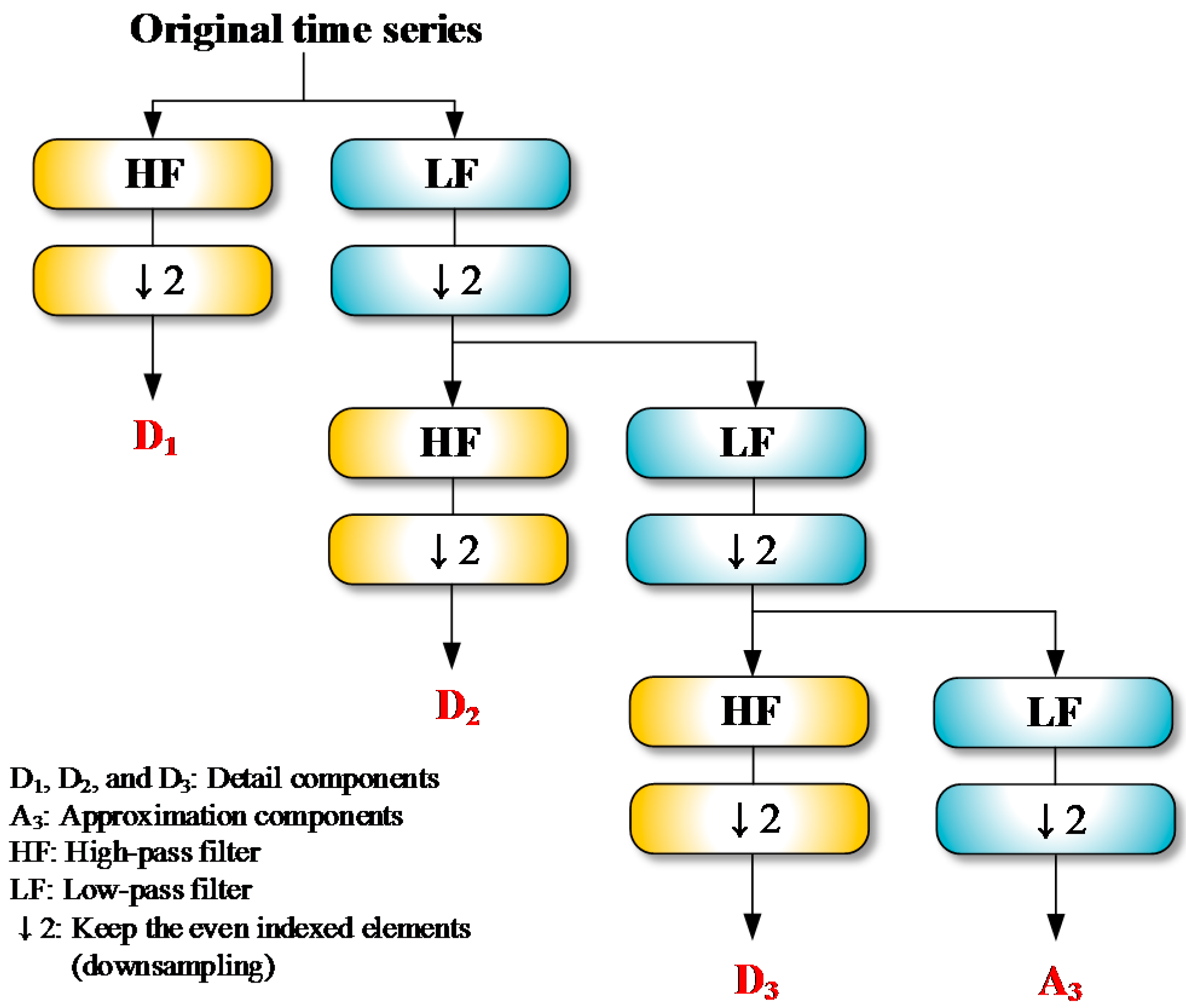
Practically, the DWT is performed by the Mallat algorithm, also known as the pyramid algorithm [66]. The key point of the algorithm is two-channel filters (also called half-band filters) which are comprised of wavelet (high-pass) filter and scaling (low-pass) filter of even width L. The main algorithm consists of circular filtering and downsampling. According to Percival and Walden [65], the wavelet and scaling coefficients for the jth decomposition level are defined as Equation (4):
where and are the elements of and , respectively. Figure 1 depicts a flowchart for three-level DWT decomposition. By utilizing the pyramid algorithm, three details (D1, D2 and D3) and an approximation (A3) are produced from an original time series. Details on the DWT can be found in Percival and Walden [65].
2.2. Variational Mode Decomposition (VMD)
VMD is a fully adaptive and non-recursive algorithm for time-frequency signal analysis. Using the VMD, an original time series f is decomposed into K IMFs. According to Dragomiretskiy and Zosso [55], the constrained variational formulation for yielding the IMFs can be written as Equation (5).
where = the Dirac function; ; = the distance; = the center frequency; * = the convolution; the kth IMF; = the non-decreasing function; and = the non-negative function. The constrained variational formulation is changed to the following unconstrained one by introducing an augmented Lagrangian method [55,67]:
where = the augmented Lagrangian, = the Lagrange multiplier, and = the scalar product of a and b.
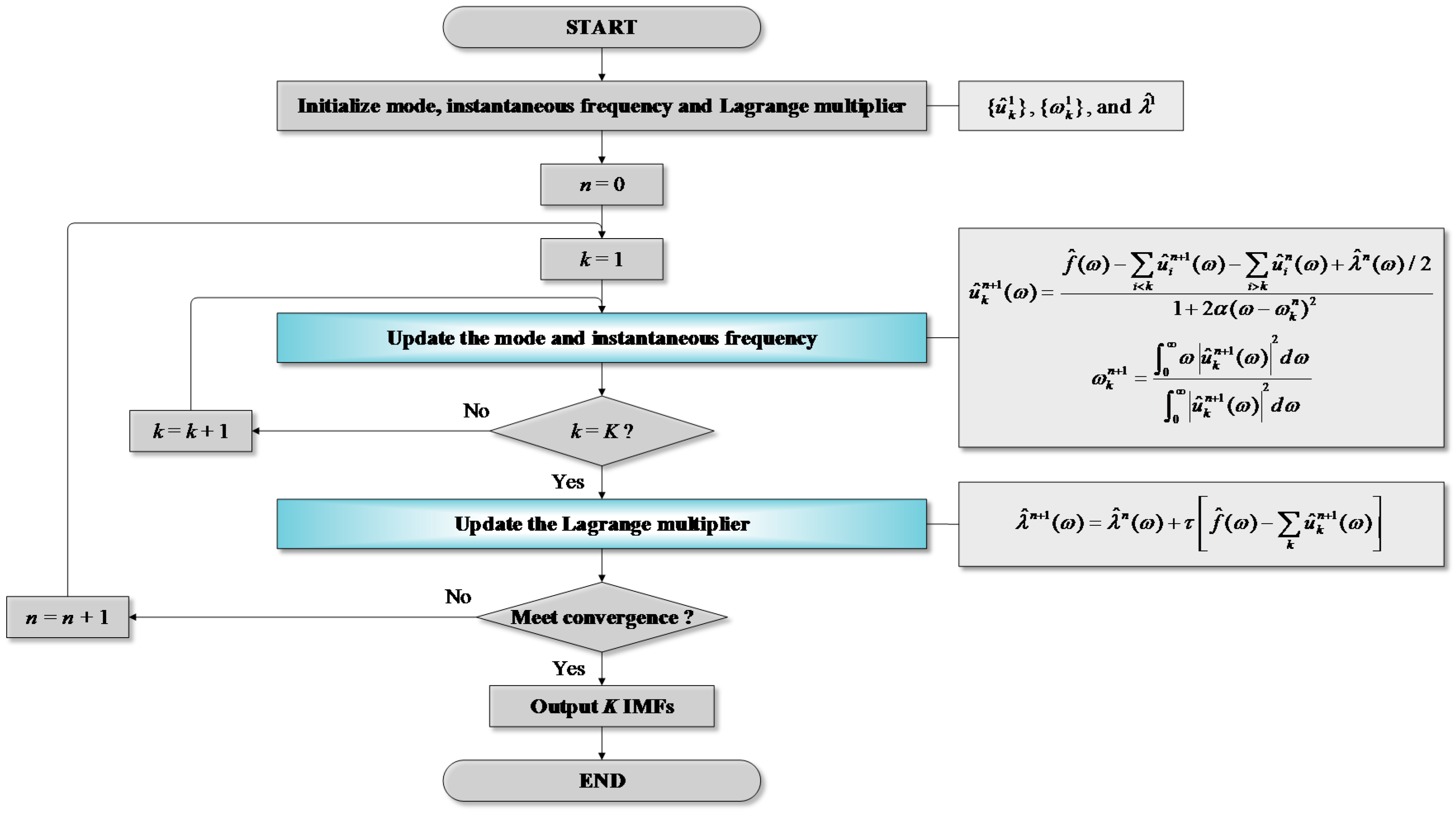
The saddle point (also called minimax point) of the L is then obtained by updating , , and in a sequence of iterative sub-optimizations using the alternate direction method of multipliers (ADMM) [68]. Compared with Newton’s method and sequential quadratic programming which are local convergence methods, the ADMM is globally convergent, robust and fast. Moreover, parallel computing becomes possible and computational cost can be greatly reduced since the ADMM can decouple a large problem into a series of sub-problems [69]. The final updated formulations can be expressed as Equations (7)–(9) [55].
where ^ = the Fourier transform, n = the iteration number, = the quadratic penalty factor, and = the time step of the dual ascent. Figure 2 shows a flowchart for the VMD. Details on the VMD can be found in Dragomiretskiy and Zosso [55].
2.3. Extreme Learning Machine (ELM)
ELM is a non-iterative and least square-based learning algorithm for training single-hidden layer feed-forward neural networks (SLFNs) effectively [70]. As stated in Huang et al. [70], the parameters of hidden layer (weights and biases) are generated randomly, and the SLFN is reduced to the linear system as Equations (10)–(13).
where H = the output matrix for the hidden layer, β = the output weight matrix; T = the target data matrix; h = the activation function, = the weight vectors between the ith hidden neuron and input neurons; = the arbitrary distinct samples, = the bias of ith hidden neuron; = the weight vectors between the ith hidden neuron and output neurons, and L = the number of hidden neurons.
Unlike the conventional ANN, the β is estimated analytically utilizing the least-square method. The optimal solution for β can be obtained by inverting the H as follows [70]:
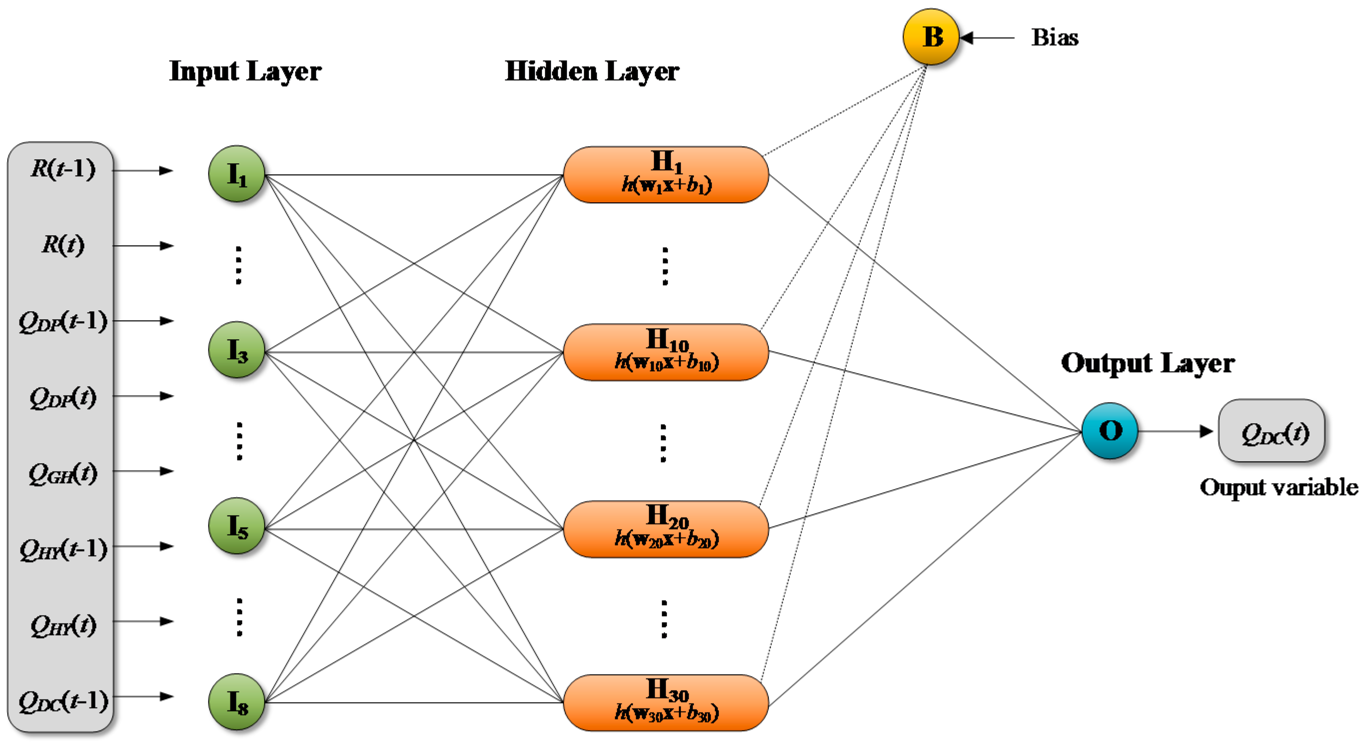
where is the Moore-Penrose generalized inverse of H, and is the inverse of the covariance matrix of H. Figure 3 shows an example of ELM model structure comprised of eight (input), 30 (hidden), and one (output) neurons, respectively. Huang et al. [70] can be referred for more details on the ELM.
2.4. Least Squares Support Vector Regression (LSSVR)
LSSVR, which is a least-squares version of standard SVR, is a kernel-based statistical learning algorithm. The SVR performs a quadratic optimization involving inequality constraints and a ε-insensitive loss function, whereas the LSSVR uses equality constraints and a least-squares loss function and solves a system of linear equations instead of the quadratic optimization. When a training set is given, the LSSVR can be written as Equation (15) [71].
where = the input data, p = the number of input patterns, = the target data, N = the data length, = the weight vector; = the dimension of a Hilbert space , = the mapping from the input space to the high dimensional feature spaces, and = the bias term.
From the research of Suykens et al. [71], the LSSVR can be converted into the primal optimization form as Equation (16).
where is the slack variable and is the regularization parameter. The Equation (16) is solved by constructing the following Lagrangian [71]:
where is the Lagrange multiplier. The Equation (17) can be solved using the partial differentiation for w, b, ei, and αi. The solution of α and b can be obtained by Equation (18) after removing the variables w and ei [71].
where , , and . Finally, the LSSVR can be expressed as the following equation [71]:
where is the kernel function that is symmetric and continuous positive definite. The typical kernels which can be utilized in the LSSVR include linear, polynomial, sigmoid, and radial basis function (RBF). For regression problems, the following RBF is generally applied [72]:
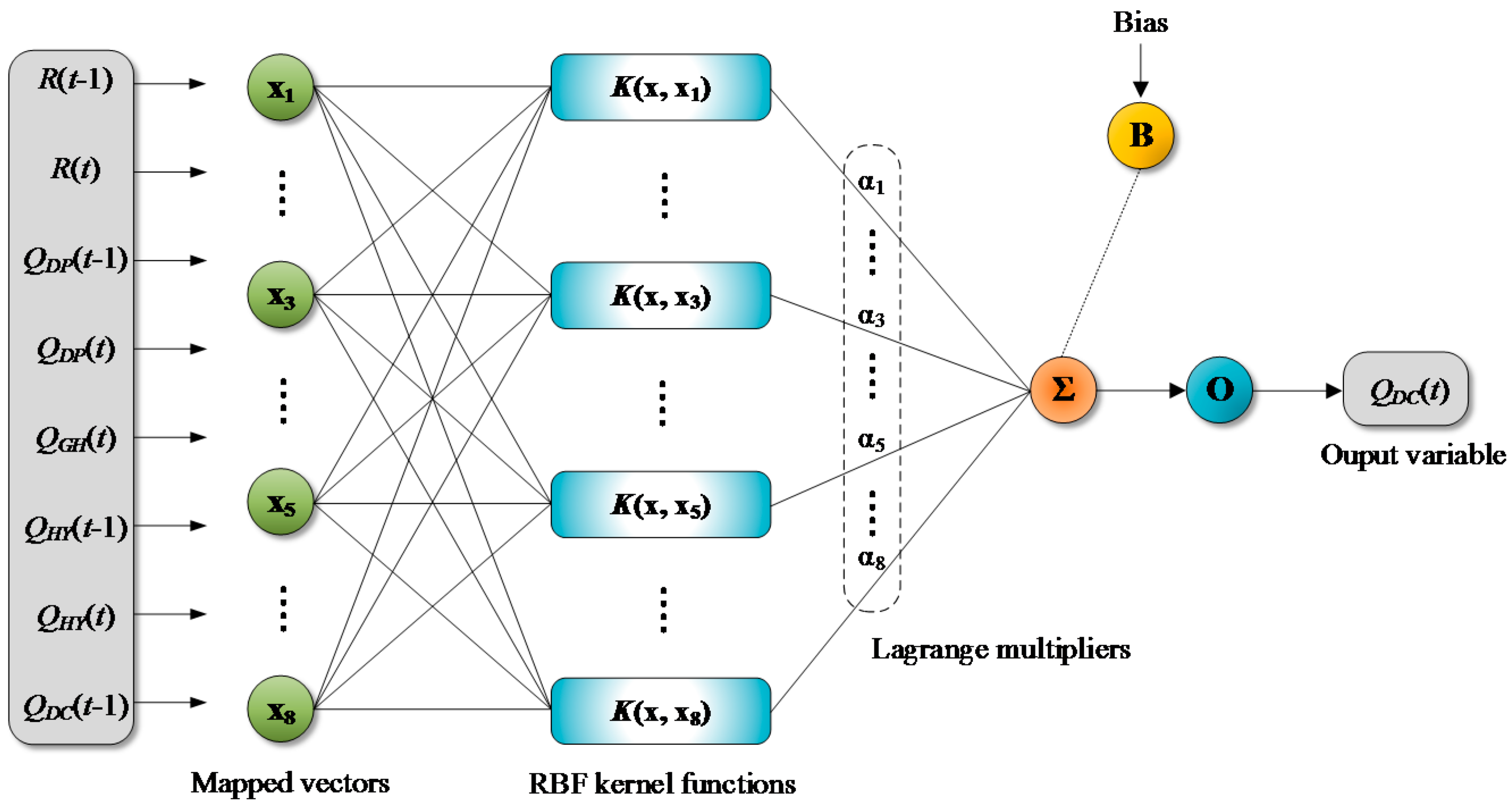
where is the parameter of RBF kernel, also called the width parameter. RBF kernel function has advantages compared with other kernel functions including linear, sigmoid, and polynomial kernel functions in terms of nonlinear mapping capability, parameter number, numerical limiting conditions, global superiority, and positive definite [73]. Furthermore, linear kernel function is effective only for linear problems, sigmoid kernel function is not applied widely, and polynomial kernel function suffers from computational difficulties [74]. On the other hand, RBF kernel function can be used for any problems as long as the parameter is selected appropriately [75]. Figure 4 shows an example of LSSVR model structure. Details on the LSSVR can be found in Suykens et al. [71].
2.5. Artificial Neural Network (ANN)
ANN is an artificial intelligent computing system that is a collection of linked layers comprised of multiple nodes called neurons analogous to the biological neural network system. Multilayer perceptron (MLP), which is a nonparametric estimator and the most widely applied ANN model, is a feedforward ANN with intermediate layers called hidden layers to implement nonlinear discriminants for classification and approximate nonlinear function for regression [76]. As seen in Figure 5, the MLP has three-layer architecture generally.
The MLP can be expressed as follows [15]:
where and = the input and output vectors, respectively, L = the number of hidden neurons, h = the activation function (also called the transfer function), and = the connection weights for the hidden and output layers, respectively, and = the biases for the hidden and output layers, respectively, and N = the data length. The parameters can be adjusted iteratively using learning algorithms such as backpropagation (BP) algorithm. Detailed information on the ANN can be found in Alpaydin [76].
2.6. VMD and DWT-based MLM Modeling
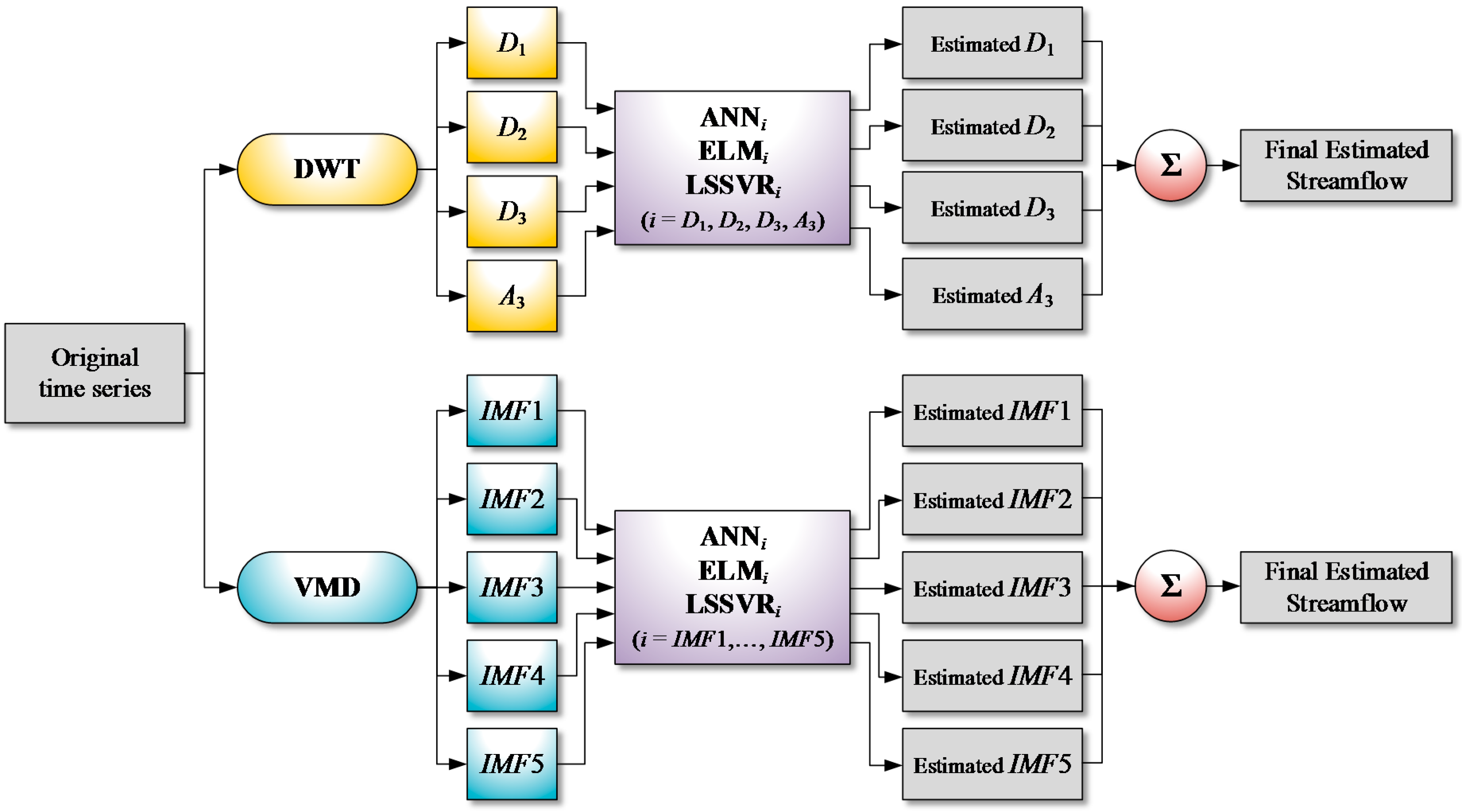
VMD-based MLMs (VMD-ELM, VMD-LSSVR, and VMD-ANN) are the hybrid models coupling the VMD and the single MLMs (ELM, LSSVR and ANN), respectively. In the same manner, DWT-based MLMs (DWT-ELM, DWT-LSSVR, and DWT-ANN) combine the DWT with the single MLMs, respectively. As shown in Figure 6, the VMD and DWT-based MLMs consist of the following three steps:
- Step 1.
- Training and testing data sets are decomposed into multiple IMFs by the VMD and an approximation and multiple details by the DWT, respectively.
- Step 2.
- For each decomposed training data set, single MLMs (ELM, LSSVR, and ANN) are developed.
- Step 3.
- The final estimates of streamflow time series are obtained by aggregating the sub-time series estimated from the single MLMs, respectively.
2.7. Quantitative Performance Indices
In this study, the model performances were assessed by efficiency and effectiveness indices. The efficiency indices include the coefficient of efficiency (CE), the index of agreement (IOA), the coefficient of determination (r2), the persistence index (PI), the root-mean-square error (RMSE), the mean absolute error (MAE), the mean squared relative error (MSRE), the mean absolute relative error (MARE), the relative volume error (RVE), and the fourth root mean quadrupled error (R4MS4E), respectively. The effectiveness indices involve the average absolute relative error (AARE) and the threshold statistics (TS). Table 1 summarizes the quantitative performance indices employed in this study. Details on the indices can be found in Jain and Srinivasulu [31] for the effectiveness indices and Dawson et al. [77] for efficiency indices, respectively. CE, r2, IOA, and PI are dimensionless indices. The indices can provide a useful comparison between different studies since they are independent on data scale. RMSE and MAE can be used as more representative measures than other indices (ex., mean square error) since they have the same unit as original data. RMSE is a good efficiency index for high flows, whereas MAE evaluates all deviations from observed values. MARE is sensitive to errors for low flows, whereas less sensitive to them for high flows. For this reason, MARE is a good efficiency index for low flows. MSRE is a good efficiency index for moderate flows. RVE is a relative index for overall volume error and can provide an indication of overall water balance. R4MS4E is a good efficiency index for high and peak flows and has the same unit as original data [77,78]. AARE and TS give appropriate weights for low, moderate, and high flows, and it has been reported that they can provide better performance evaluation [31].
3. Study Area and Observed Data
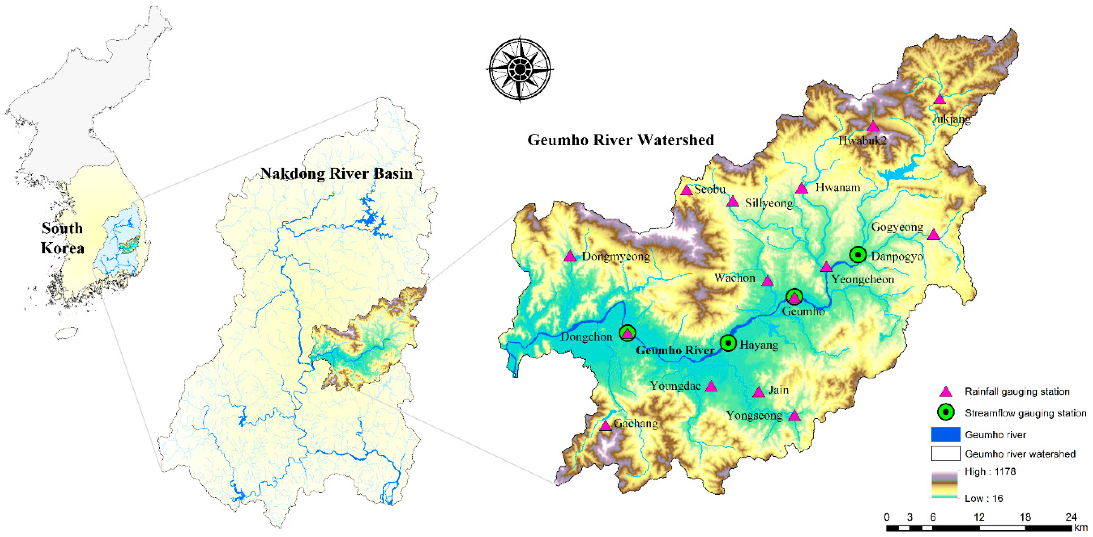
The study area for investigating the model performance is the Geumho River Watershed, South Korea. Sufficient and reliable observed data are essential for developing MLMs. The Geumho River Watershed has a number of gauging stations with long-term observation periods of more than 20 years. Moreover, since the gauging stations have been strictly managed by the Ministry of Land, Infrastructure and Transport, the quality and reliability of their data is good. The Geumho River Watershed is thus adequate as study area in this study in terms of the number of gauging stations and the availability and reliability of observed data. Figure 7 displays the study area and locations of gauging stations.
The watershed is in the central-eastern part of the Nakdong River Basin which is the second largest among the river basins of South Korea. The watershed has an area of 2092.4 km2, an average watershed elevation of 235.4 m, an average watershed slope of 33.6%, and a stream length of 119.0 km [79]. To develop the hybrid and single MLMs, daily streamflow and rainfall data were gathered from four streamflow and 15 rainfall gauging stations, respectively (see Figure 7). The data are available from the Water Management Information System (WAMIS) [79] which is a web portal information service that has been operated for providing and managing the water resources and environmental information of South Korea effectively. The areal mean rainfall (AMR) time series was calculated from the collected rainfall data using Thiessen polygon method [80]. The AMR and streamflow time series were utilized for model training and testing. These time series were scaled to the range of [0,1] for efficient model training [78] and grouped into two data sets: training (2001-2010, data length = 3652) and testing data sets (2011–2014, data length = 1461).
4. Results and Discussion
4.1. Development of Hybrid and Single MLMs
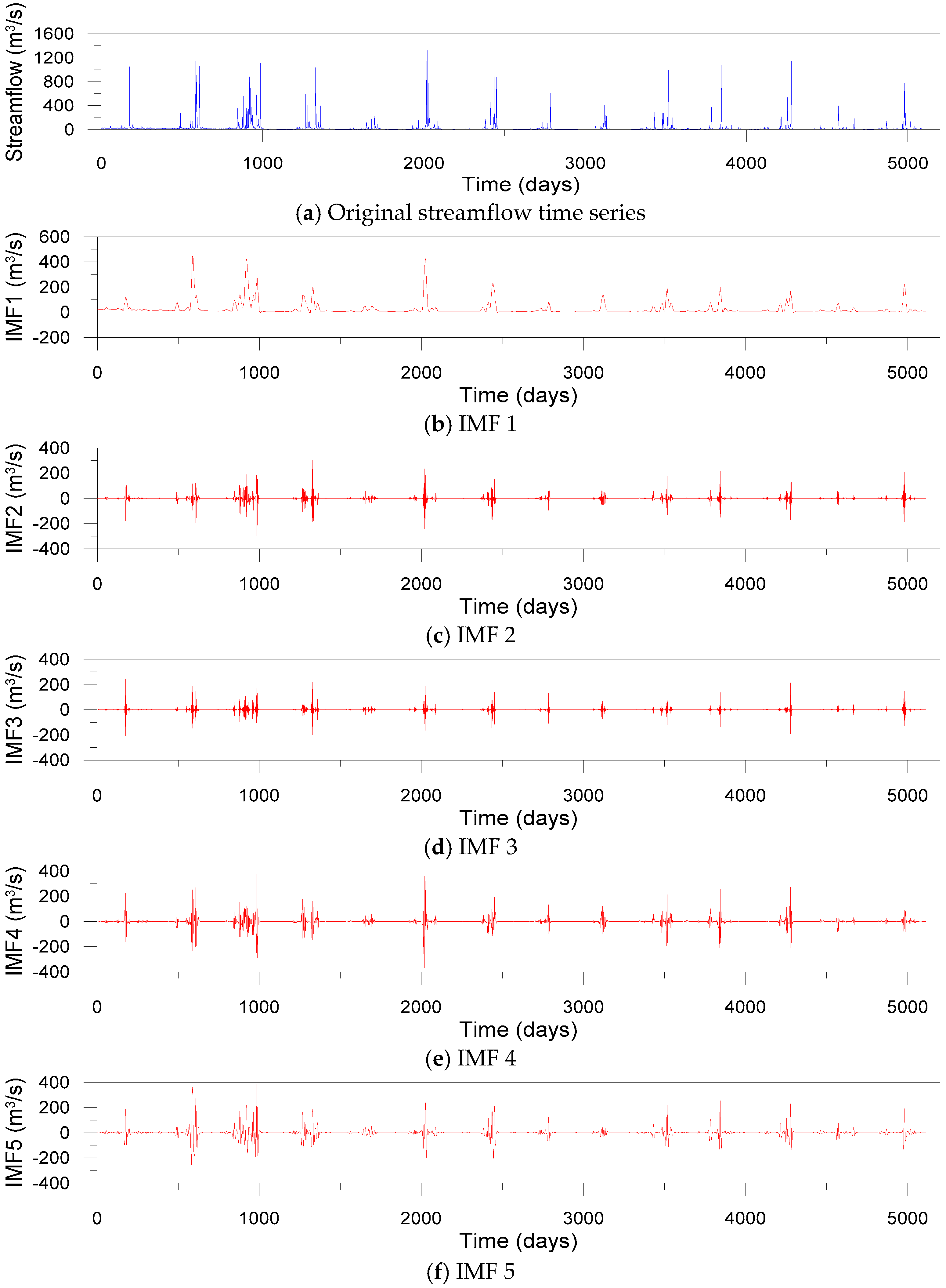
To decompose input and target time series by the VMD, the number of IMFs (K) and the quadratic penalty factor (α) should be determined beforehand. In this study, the parameters, K and α, were determined according to the following steps:
- Step 1.
- Decompose input and target time series into IMFs for different K = [1, 20] and α = [5, 2000].
- Step 2.
- Add up the IMFs for each of the K and α values again and estimate the values of correlation coefficient (r) for the reconstructed and original time series.
- Step 3.
- Select the sets of K and α values for .
- Step 4.
- Select the optimal K and α values producing the best performance of VMD-based MLMs.
Based on the above method, K = 5 and α = 10 were determined in this study. Figure 8 shows five IMFs decomposed by the VMD for daily streamflow data observed at the Dongchon streamflow gauging station.
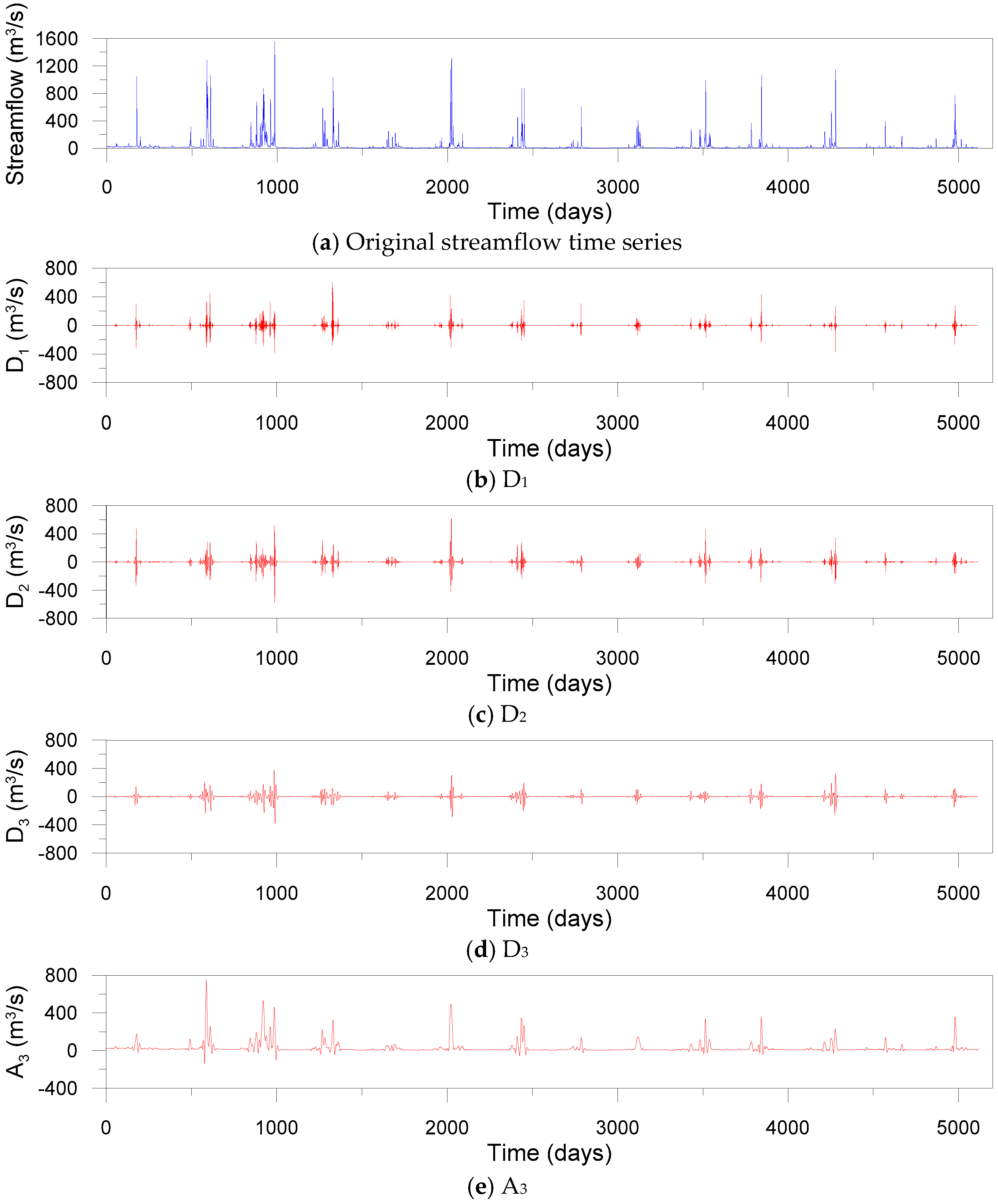
To decompose input and target time series by the DWT, the optimal level of decomposition (L) should be first selected. In this study, Equation (22) [81] was used for determining the L value:
where N is the length of time series, returns the integer portion of k, and k is a real number. Using Equation (22), L = 3 was determined in this study. The determination of decomposition level using Equation (22) has been adopted in many previous studies [81,82,83,84,85,86]. Although the decomposition level can be also selected using a trial-and-error method, it is computationally burdensome and time-consuming. Furthermore, a mother wavelet should be selected before performing the DWT. The performance of DWT-based MLMs is dependent on the mother wavelet [6]. For each model, the optimal mother wavelet producing the best model performance was selected. As a result, the optimal mother wavelets were chosen as d12 for DWT-ELM, d12 for DWT-LSSVR, and d18 for DWT-ANN, respectively. Figure 9 shows an approximation and three details decomposed by the DWT for daily streamflow data observed at the Dongchon streamflow gauging station.
In developing rainfall-runoff models using MLMs, one of the most important modeling steps is to select the appropriate input variables [78]. Table 2, Table 3 and Table 4 summarize the input sets for VMD-based MLMs, DWT-based MLMs, and single MLMs, respectively. The input sets can be set up based on the following steps in this study:
- Step 1.
- Select the potential influencing variables based on the lag times of input variables determined by autocorrelation function (ACF), partial autocorrelation function (PACF), cross-correlation function (CCF), and average mutual information (AMI).
- Step 2.
- Select five input sets for each model utilizing the variables selected in step 1 and all-possible-regression method [87], where Mallows’s Cp and adjusted r2 [87] are used as the criteria for selecting the sets. The Mallows’s Cp is minimized when the input set consists of only statistically significant variables. The adjusted r2 helps prevent overfitting since a penalty is given when adding variables to a model [87,88].
- Step 3.
- Select the optimal input set producing the best performance for each model based on quantitative performance indices.
The critical modeling phase for developing the MLP and ELM models is to select the optimal number of hidden neurons. The model performances are affected by the number of hidden neurons. The optimal number was selected utilizing a trial-and-error approach [6,89]. Furthermore, the logistic sigmoid function (also known as the log-sigmoid), which has been applied in most hydrological neural network modeling [78], was employed for calculating the output of each neuron for the MLP and ELM models, and BP algorithm was used for training the MLP model. For MLP, the training parameters (learning rate and momentum rate) mainly affect the convergent speed of learning procedure, not the model performance. Larger learning rate leads to unstable oscillation and local minimum [90,91]. Although the momentum rate is used for filtering out the oscillation, it cannot be removed completely. When the learning parameters are small, they have a minor effect on the performance although the convergence time is increased. According to Dai and MacBeth [92], the learning parameters can be obtained by a trial-and-error approach, but it is time-consuming, and they marginally affect the performance. Therefore, it is not necessary to take a lot of effort to select the optimal values, and it is more efficient to select appropriate small learning parameters considering the computation speed (convergence speed). In this study, the default values of learning parameters suggested by Zell et al. [93] were used.
For the LSSVR modeling, selecting the regularization and kernel parameters is one of the significant modeling steps. The parameters should be selected in advance. Coupled simulated annealing (CSA) and derivative-free simplex search (DSS) [94,95] were used for selecting the optimal parameters. In the parameter optimization, the CSA determines the initial values, and the DSS performs the fine-tuning [96]. Optimization algorithms, including gradient-based techniques, simulated annealing, genetic algorithms, particle swarm optimization, etc., can be used for selecting the optimal parameters. The gradient-based methods have limitations when the cost function is non-differential and the computation cost for large-scale problems is high. Additionally, the method suffers from performance degradation when there is multimodality, multidimensionality, and many local minima in search space. Global optimization algorithms including simulated annealing, genetic algorithms and particle swarm optimization have the advantage that they can escape from multiple local minima. However, global optimization algorithms have high computational burdensome and very slow convergence since they require very many evaluations for cost function to reach the global optimum. Moreover, they are sensitive to the initial parameters [95]. On the other hand, CSA features fast convergence speed and can reduce the sensitivity for the initial parameters although there is a tradeoff between the number of evaluations for cost function and the quality of the final solutions. The tradeoff problem can be resolved by performing a fine tuning by the DSS. Thus, the coupled CSA and DSS result in better performance and more optimal solutions [97,98].
Considering the above modeling strategies, three VMD-based MLMs (VMD-ELM, VMD-LSSVR and VMD-ANN), three DWT-based MLMs (DWT-ELM, DWT-LSSVR and DWT-ANN) and three single MLMs (ELM, LSSVR, and ANN) were developed. Table 5 shows the optimal model architectures. For ANN, ELM, VMD-ANN, VMD-ELM, DWT-ANN, and DWT-ELM models, the digits represent the number of input, hidden, and output neurons, respectively. For LSSVR, VMD-LSSVR, and DWT-LSSVR models, the digits represent the number of input nodes, RBF kernel functions, and output nodes, respectively.
4.2. Performance Assessment
As stated in the Introduction chapter, this study aims at examining the performances of VMD-based MLMs for daily rainfall-runoff modeling and comparing them with those of DWT-based and single MLMs. The model performances were evaluated using the quantitative performance indices which measure the model efficiency and effectiveness. The results are summarized in Table 6.
When the values of CE, IOA, r2 and PI are close to one and the values of RMSE, MAE, MSRE, MARE, RVE, and R4MS4E are close to zero, it indicates that a model achieves better efficiency compared with other models. Also, when lower AARE and higher TS are produced by a model, it represents that the model has better effectiveness.
In comparing the performances of VMD-based and single MLMs, VMD-based MLMs yielded better efficiency and effectiveness indices than ELM, LSSVR and ANN models, respectively. It can be indicated from this result that the combination of VMD and single MLMs can improve the performances of single MLMs in terms of efficiency and effectiveness. Also, the performances of VMD-based MLMs were compared with those of DWT-based MLMs. As a result, VMD-ELM and VMD-LSSVR models provided better efficiency, whereas VMD-ELM and DWT-LSSVR models performed better in terms of effectiveness. When both model efficiency and effectiveness were considered, the VMD-ELM and VMD-LSSVR models achieved the better performance. On the other hand, VMD-ANN model yielded poor efficiency and effectiveness as compared with DWT-ANN model. These results revealed that the VMD was able to enhance the performances of ELM and LSSVR models, whereas the DWT was more suitable to improve the performance of ANN model than the VMD for daily rainfall-runoff modeling. Among all the models, the top three models with the best efficiency and effectiveness can be identified as VMD-ELM, VMD-LSSVR, and DWT-ELM models, respectively. These results indicated that the VMD provided better efficiency and effectiveness than the DWT for daily rainfall-runoff modeling utilizing MLMs, and the performance reliability was also dependent on the MLMs.
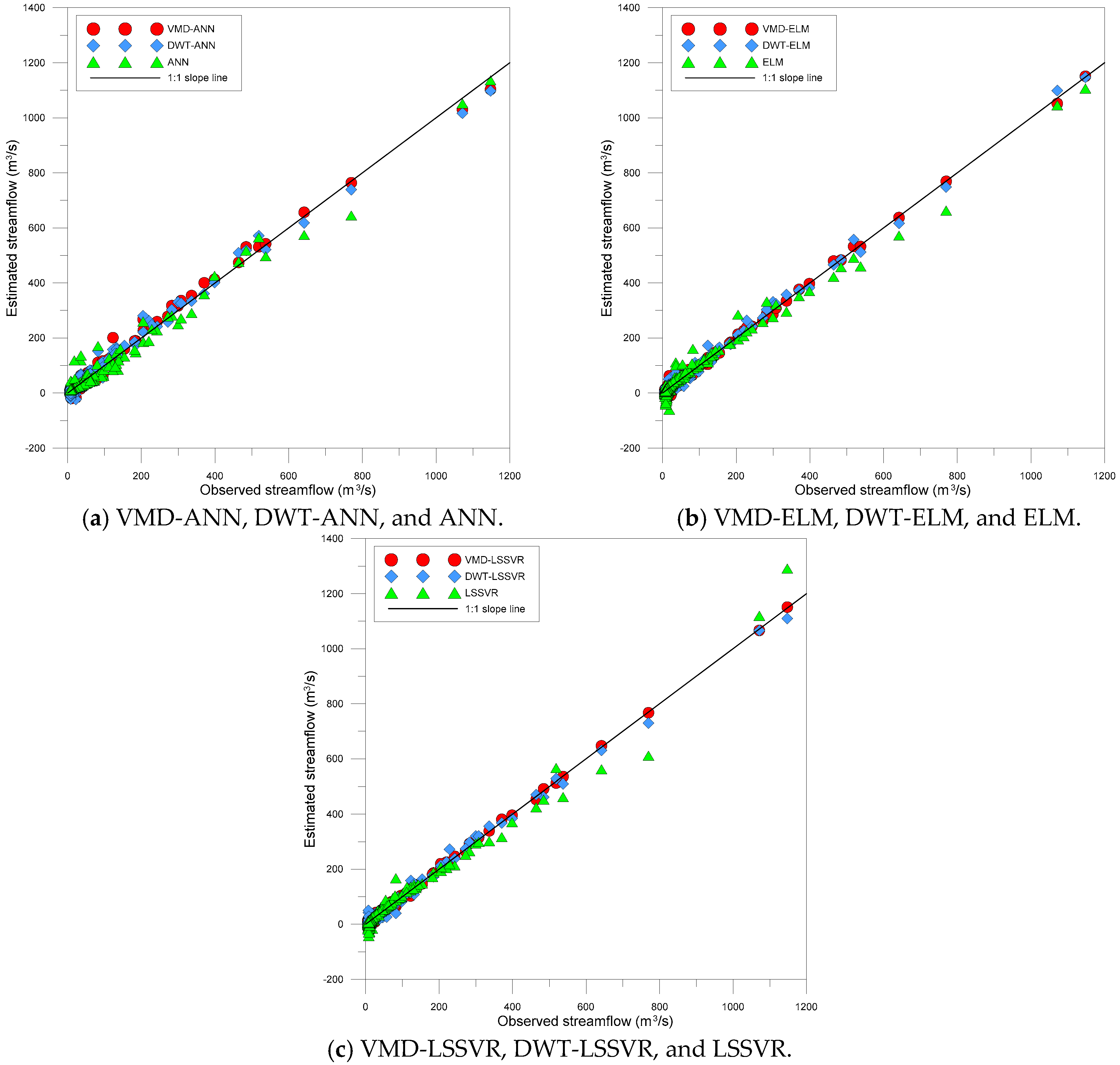
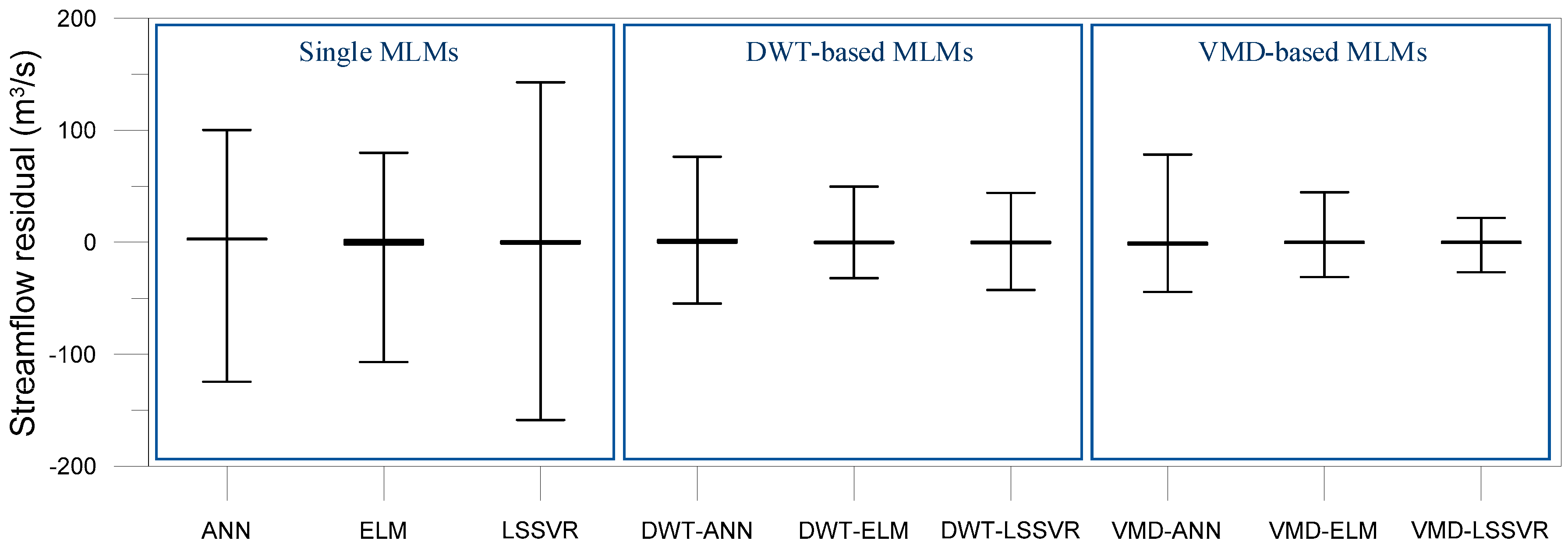
Figure 10 and Figure 11 show the scatter plots and the residual boxplots for the VMD-based, DWT-based, and single MLMs, respectively. The plots provide the graphical comparison of model accuracy. The scatter plots represent the degree of correlation and dispersion between estimated and observed values, whereas the residual boxplots depict the distribution of residuals that are the differences between estimated and observed values.
From Figure 10, it was observed that the scatter points of the VMD-based and DWT-based MLMs were closer to the 1:1 slope line compared with the single MLMs. This indicated that the VMD-based and DWT-based MLMs provided better accuracy than the single MLMs. From Figure 11, it was evident that the overall residual ranges (the maximum residual minus the minimum residual) of the single MLMs were larger than those of the VMD-based and DWT-based MLMs, whereas the interquartile residual ranges (the third quartile minus the first quartile for residual) for all models were similar and small. It can be found from the figures that the single MLMs produced worse results than the VMD-based and DWT-based MLMs for extreme (low and high) streamflow even if all models provided accurate results for almost streamflow data. Especially, as seen in Figure 10, the VMD-based and DWT-based MLMs models yielded the best accurate streamflow values compared with the single MLMs for higher streamflow.
Based on model performance evaluation and graphical comparison, VMD-based and DWT-based MLMs produced better results than single MLMs in daily rainfall-runoff modeling. These results are consistent with those of previous studies dealing with hybrid modeling for rainfall-runoff process [6,47,99,100,101]. Single MLMs (e.g., ANN, ELM, and LSSVR) represent a natural limitation in terms of nonstationary hydrologic time series modeling even if they can model nonlinear hydrologic time series effectively [102,103]. However, in case of VMD-based and DWT-based hybrid modeling, VMD and DWT decompose an original time series into time-frequency features (details and approximation for DWT, and IMFs for VMD), and the features are then used for the inputs of single MLMs. Since the MLMs utilize the training data with more simple structure for each scale obtained by time series decomposition in the training process, they can learn the data pattern more effectively. These characteristics can reduce the effects of nonlinearity and nonstationarity embedded in the original time series. Therefore, VMD-based and DWT-based hybrid rainfall-runoff models can deal with nonlinear and nonstationary hydrologic time series more effectively and also improve the model performance.
In this study, ANN, VMD-ANN, and DWT-ANN models were trained using backpropagation algorithm which has been widely applied in hydrological applications. Chau [104] proposed a split-step PSO algorithm which combines particle swarm optimization for global search and Levenberg-Marquardt algorithm for fast local search in river stage forecasting. The algorithm provided more improved results in terms of computation time and accuracy. Similarly, in ANN-based rainfall-runoff modeling, using the enhanced learning algorithm may help improve the computation time and accuracy of ANN models. Furthermore, for VMD- and DWT-based ANN modeling, VMD and DWT increase the number of input features for ANN models greatly since sub-time series decomposed by VMD and DWT are used as the training dataset of ANN models. The enhanced learning algorithm may also improve the computation time and accuracy of VMD-ANN and DWT-ANN models. Therefore, a rainfall-runoff modeling combining VMD (or DWT), split-step PSO, and ANN can be suggested as a future study. For LSSVR, VMD-LSSVR, and DWT-LSSVR models, the optimal parameters were determined using coupled CSA and DSS algorithms in this study. The algorithms feature enhanced computation speed and accuracy compared with conventional global optimization algorithms. However, the coupled CSA and DSS algorithms may be more enhanced if they utilize the parallel computing concept using multiple computers and parallel genetic algorithm proposed by Cheng et al. [105] or graphics processing unit (GPU)-based computing (ex., Zhou and Tan [106]) which has been getting the spotlight recently. These methods can help an optimization algorithm to search multidimensional solution space efficiently since the enhanced computing ability can significantly reduce the computation time for optimization. In this study, original time series were decomposed into sub-time series by VMD and DWT. In contrast, Taormina et al. [107] split hydrograph into baseflow and excess flow components using digital filter, and then trained modular neural networks for the components, respectively. Wu and Chau [108] used singular spectrum analysis for the decomposition and analysis of original time series. Combining the advantages of these methods may help improve the performance of rainfall-runoff MLMs. In other words, it can be suggested to divide an original time series into baseflow and excess flow components using the baseflow separation method, decompose them into sub-time series by applying VMD or DWT to each component, and then utilize the sub-time series as a training dataset for modeling rainfall-runoff MLMs.
5. Conclusions
In this study, two different conjunction models, VMD-ELM and VMD-LSSVR, are developed for daily rainfall-runoff modeling in the Geumho River Watershed, South Korea, and their performances are investigated. The performances of the coupled models are evaluated utilizing the quantitative performance indices, namely, efficiency and effectiveness indices. The results are compared with those of VMD-ANN, DWT-based MLMs (DWT-ELM, DWT-LSSVR, and DWT-ANN), and single MLMs (ELM, LSSVR, and ANN). As a result, the VMD and DWT-based MLMs perform better than the single MLMs. The VMD-ELM and VMD-LSSVR models yield slightly better performance than the DWT-ELM and DWT-LSSVR models, whereas the DWT-ANN model produces slightly better performance as compared with the VMD-ANN model. Considering efficiency and effectiveness, the VMD-ELM and VMD-LSSVR models achieve the best performance. These results confirm that the VMD can enhance the performances of single MLMs for daily rainfall-runoff modeling, and the performances of VMD-based MLMs are dependent on the combination of single MLMs. Therefore, the VMD can be a novel alternative technique for hybrid rainfall-runoff modeling based on time series decomposition.
In this study, two VMD-based hybrid MLMs, VMD-ELM and VMD-LSSVR, are proposed for daily rainfall-runoff modeling. This study deals with rainfall-runoff modeling on daily basis using VMD-based hybrid MLMs. However, it is also necessary to investigate the performances of VMD-based rainfall-runoff models on weekly, monthly, and annual basis for effective river basin management, water supply and allocation, and reservoir planning and operation. Moreover, this study has the limitation that it employs rainfall and streamflow as predictors for rainfall-runoff modeling and does not consider runoff components (surface, subsurface, and groundwater flow components), hydro-physical elements (evapotranspiration, infiltration, etc.), and human-made factors. It can be suggested as future studies to investigate VMD-based rainfall-runoff modeling considering runoff components and various factors, effective variable selection methods, comparison with different time series decomposition methods and MLMs; hybrid learning algorithm combining global and local search algorithms, parameter optimization using GPU-based parallel computing, and rainfall-runoff MLMs using baseflow separation and time series composition methods.
Author Contributions
Y.S. designed this research, reviewed the literature, and analyzed the data and developed analysis tool and models. S.K. reviewed state of the art reports and literatures, optimized the developed models, and revised the draft manuscript. V.P.S. supervised research processes and finalized the manuscript.
Funding
This research received no external funding.
Acknowledgments
The authors would like to reveal our extreme appreciation and gratitude to the Water Management Information System (WAMIS), South Korea. This is with regard of providing the metrological information. In addition, the authors also thank the editors and reviewers for their admirable revision and scientific suggestions sincerely.
Conflicts of Interest
The authors declare no conflict of interest.
References
- Besaw, L.E.; Rizzo, D.M.; Bierman, P.R.; Hackett, W.R. Advances in ungauged streamflow prediction using artificial neural networks. J. Hydrol. 2010, 386, 27–37. [Google Scholar] [CrossRef]
- Yassen, Z.M.; Jaafar, O.; Deo, R.C.; Kisi, O.; Adamowski, J.; Quilty, J.; El-Shafie, A. Stream-flow forecasting using extreme learning machines: A case study in a semi-arid region in Iraq. J. Hydrol. 2016, 542, 603–614. [Google Scholar] [CrossRef]
- Singh, H.; Sankarasubramanian, A. Systematic uncertainty reduction strategies for developing streamflow forecasts utilizing multiple climate models and hydrologic models. Water Resour. Res. 2014, 50, 1288–1307. [Google Scholar] [CrossRef] [Green Version]
- Wang, W. Stochasticity, Nonlinearity and Forecasting of Streamflow Processes; IOS Press: Amsterdam, The Netherlands, 2006. [Google Scholar]
- Shalamu, A. Monthly and Seasonal Streamflow Forecasting in the Rio Grande Basin. Ph.D. Thesis, New Mexico State University, Las Cruces, NM, USA, 2009. [Google Scholar]
- Seo, Y.; Kim, S.; Kisi, O.; Singh, V.P. Daily water level forecasting using wavelet decomposition and artificial intelligence techniques. J. Hydrol. 2015, 520, 224–243. [Google Scholar] [CrossRef]
- Kisi, O. Streamflow forecasting and estimation using least square support vector regression and adaptive neuro-fuzzy embedded fuzzy c-means clustering. Water Resour. Manag. 2015, 29, 5109–5127. [Google Scholar] [CrossRef]
- Toth, E. Classification of hydro-meteorological conditions and multiple artificial neural networks for streamflow forecasting. Hydrol. Earth Syst. Sci. 2009, 13, 1555–1566. [Google Scholar] [CrossRef] [Green Version]
- Shiri, J.; Kisi, O. Short-term and long-term streamflow forecasting using a wavelet and neuro-fuzzy conjunction model. J. Hydrol. 2010, 394, 486–493. [Google Scholar] [CrossRef]
- Rasouli, K.; Hsieh, W.W.; Cannon, A.J. Daily streamflow forecasting by machine learning methods with weather and climate inputs. J. Hydrol. 2012, 414–415, 284–293. [Google Scholar] [CrossRef]
- Sudheer, C.; Maheswaran, R.; Panigrahi, B.K.; Mathur, S. A hybrid SVM-PSO model for forecasting monthly streamflow. Neural Comput. Appl. 2014, 24, 1381–1389. [Google Scholar] [CrossRef]
- Yang, T.; Asanjan, A.A.; Welles, E.; Gao, X.; Sorooshian, S.; Liu, X. Developing reservoir monthly inflow forecasts using artificial intelligence and climate phenomenon information. Water Resour. Res. 2017, 53, 2786–2812. [Google Scholar] [CrossRef]
- Okkan, U.; Serbes, Z.A. Rainfall-runoff modeling using least squares support vector machines. Environmetrics 2012, 23, 549–564. [Google Scholar] [CrossRef]
- Shabri, A.; Suhartono. Streamflow forecasting using least-squares support vector machines. Hydrol. Sci. J. 2012, 57, 1275–1293. [Google Scholar] [CrossRef] [Green Version]
- Lima, A.R.; Cannon, A.J.; Hsieh, W.W. Forecasting daily streamflow using online sequential extreme learning machines. J. Hydrol. 2016, 537, 431–443. [Google Scholar] [CrossRef]
- Rezaie-Balf, M.; Kisi, O. New formulation for forecasting streamflow: Evolutionary polynomial regression vs. extreme learning machine. Hydrol. Res. 2017, 49, 939–953. [Google Scholar] [CrossRef]
- ASCE Task Committee. Artificial neural networks in hydrology. I: Preliminary concepts. J. Hydrol. Eng. 2000, 5, 115–123. [Google Scholar] [CrossRef]
- ASCE Task Committee. Artificial neural networks in hydrology. II: Hydrological applications. J. Hydrol. Eng. 2000, 5, 124–137. [Google Scholar] [CrossRef]
- Yaseen, Z.M.; El-shafie, A.; Jaafar, O.; Afan, H.A.; Sayl, K.N. Artificial intelligence based models for stream-flow forecasting. J. Hydrol. 2015, 530, 829–844. [Google Scholar] [CrossRef]
- Fahimi, F.; Yassen, Z.M.; El-shafie, A. Application of soft computing based hybrid models in hydrological variables modeling: A comprehensive review. Theor. Appl. Climatol. 2017, 128, 875–903. [Google Scholar] [CrossRef]
- Fotovatikhah, F.; Herrera, M.; Shamshirband, S.; Chau, K.; Ardabili, S.F.; Piran, M.J. Survey of computational intelligence as basis to big flood management: Challenges, research directions and future work. Eng. Appl. Comput. Fluid 2018, 12, 411–437. [Google Scholar] [CrossRef]
- Wu, C.L.; Chau, K.W.; Li, Y.S. Predicting monthly streamflow using data–driven models coupled with data-preprocessing techniques. Water Resour. Res. 2009, 45, W08432. [Google Scholar] [CrossRef]
- Wu, C.L.; Chau, K.W. Data-driven models for monthly streamflow time series prediction. Eng. Appl. Artif. Intell. 2010, 23, 1350–1367. [Google Scholar] [CrossRef] [Green Version]
- Gousheh, M. Assessment of input variables determination on the SVM model performance using PCA, Gamma test, and forward selection techniques for monthly stream flow prediction. J. Hydrol. 2011, 401, 177–189. [Google Scholar] [CrossRef]
- Saghafian, B.; Anvari, S.; Morid, S. Effect of Southern Oscillation Index and spatially distributed climate data on improving the accuracy of Artificial Neural Network, Adaptive Neuro-Fuzzy Inference System and K-Nearest Neighbour streamflow forecasting models. Expert Syst. 2013, 30, 367–380. [Google Scholar] [CrossRef]
- Corzo, G.; Solomatine, D. Knowledge-based modularization and global optimization of artificial neural network models in hydrological forecasting. Neural Netw. 2007, 20, 528–536. [Google Scholar] [CrossRef] [PubMed]
- Asadi, S.; Shahrabi, J.; Abbaszadeh, P.; Tabanmehr, S. A new hybrid artificial neural networks for rainfall-runoff process modeling. Neurocomputing 2013, 121, 470–480. [Google Scholar] [CrossRef]
- Yang, C.-C.; Chen, C.-S. Application of integrated back-propagation network and self organizing map for flood forecasting. Hydrol. Process. 2009, 23, 1313–1323. [Google Scholar] [CrossRef]
- Wu, M.-C.; Lin, G.-F.; Lin, H.-Y. Improving the forecasts of extreme streamflow by support vector regression with the data extracted by self-organizing map. Hydrol. Process. 2012, 28, 386–397. [Google Scholar] [CrossRef]
- Tiwari, M.K.; Chatterjee, C. Uncertainty assessment and ensemble flood forecasting using bootstrap based artificial neural networks (BANNs). J. Hydrol. 2010, 382, 20–33. [Google Scholar] [CrossRef]
- Jain, A.; Srinivasulu, S. Development of effective and efficient rainfall-runoff models using integration of deterministic, real-coded genetic algorithms and artificial neural network techniques. Water Resour. Res. 2004, 40. [Google Scholar] [CrossRef] [Green Version]
- Sedki, A.; Ouazar, D.; El Mazoudi, E. Evolving neural network using real coded genetic algorithm for daily rainfall-runoff forecasting. Expert Syst. Appl. 2009, 36 Pt 1, 4523–4527. [Google Scholar] [CrossRef]
- Cheng, C.; Niu, W.; Feng, Z.; Shen, J.; Chau, K. Daily reservoir runoff forecasting method using artificial neural network based on quantum-behaved particle swarm optimization. Water 2015, 7, 4232–4246. [Google Scholar] [CrossRef]
- Turan, M.E. Fuzzy systems tuned by swarm based optimization algorithms for predicting stream flow. Water Resour. Manag. 2016, 30, 4345–4362. [Google Scholar] [CrossRef]
- Xing, B.; Gan, R.; Liu, G.; Liu, Z. Monthly mean streamflow prediction based on bat algorithm-support vector machine. J. Hydrol. Eng. 2016, 21, 04015057. [Google Scholar] [CrossRef]
- Yassen, Z.M.; Ebtehaj, I.; Bonakdari, H.; Deo, R.C.; Mehr, A.D.; Mohtar, W.H.M.W.; Diop, L.; El-shafie, A.; Singh, V.P. Novel approach for streamflow forecasting using a hybrid ANFIS-FFA model. J. Hydrol. 2017, 554, 263–276. [Google Scholar] [CrossRef]
- Kisi, O.; Cimen, M. A wavelet-support vector machine conjunction model for monthly streamflow forecasting. J. Hydrol. 2011, 399, 132–140. [Google Scholar] [CrossRef]
- Liu, Z.; Zhou, P.; Chen, G.; Guo, L. Evaluating a coupled discrete wavelet transform and support vector regression for daily and monthly streamflow forecasting. J. Hydrol. 2014, 519 Pt D, 2822–2831. [Google Scholar] [CrossRef]
- Adamowski, J.; Sun, K. Development of a coupled wavelet transform and neural network method for flow forecasting of non-perennial rivers in semi-arid watersheds. J. Hydrol. 2010, 390, 85–91. [Google Scholar] [CrossRef]
- Moosavi, V.; Talebi, A.; Hadian, M.R. Development of a hybrid wavelet packet-group method of data handling (WPGMDH) model for runoff forecasting. Water Resour. Manag. 2017, 31, 43–59. [Google Scholar] [CrossRef]
- Napolitano, G.; Serinaldi, F.; See, L. Impact of EMD decomposition and random initialization of weights in ANN hindcasting of daily stream flow series: An empirical examination. J. Hydrol. 2011, 406, 199–214. [Google Scholar] [CrossRef]
- Huang, S.; Chang, J.; Huang, Q.; Chen, Y. Monthly streamflow prediction using modified EMD-based support vector machine. J. Hydrol. 2014, 511, 764–775. [Google Scholar] [CrossRef]
- Wang, W.; Chau, K.; Qiu, L.; Chen, Y. Improving forecasting accuracy of medium and long-term runoff using artificial neural network based on EEMD decomposition. Environ. Res. 2015, 139, 46–54. [Google Scholar] [CrossRef] [PubMed]
- Bai, Y.; Chen, Z.; Xie, J.; Li, C. Daily reservoir inflow forecasting using multiscale deep feature learning with hybrid models. J. Hydrol. 2016, 532, 193–206. [Google Scholar] [CrossRef]
- Zhang, F.; Dai, H.; Tang, D. A conjunction method of wavelet transform-particle swarm optimization-support vector machine for streamflow forecasting. J. Appl. Math. 2014, 2014, 1–10. [Google Scholar] [CrossRef]
- Dariane, A.B.; Azimi, S. Forecasting streamflow by combination of a genetic input selection algorithm and wavelet transforms using ANFIS models. Hydrol. Sci. J. 2016, 61, 585–600. [Google Scholar] [CrossRef]
- Wang, W.; Xu, D.; Chau, K.; Chen, S. Improved annual rainfall–runoff forecasting using PSO–SVM model based on EEMD. J. Hydroinform. 2013, 15, 1377–1390. [Google Scholar] [CrossRef]
- Barge, J.; Sharif, H.O. An ensemble empirical mode decomposition, self-organizing map, and linear genetic programming approach for forecasting river streamflow. Water 2016, 8, 247. [Google Scholar] [CrossRef]
- Baydaroğlu, Ő.; Koçak, K.; Duran, K. River flow prediction using hybrid models of support vector regression with the wavelet transform, singular spectrum analysis and chaotic approach. Meteorol. Atmos. Phys. 2018, 130, 349–359. [Google Scholar] [CrossRef]
- Wang, W.; Chau, K.; Xu, D.; Qiu, L.; Liu, C. The annual maximum flood peak discharge forecasting using hermite projection pursuit regression with SSO and LS method. Water Resour. Manag. 2017, 31, 461–477. [Google Scholar] [CrossRef]
- Gokhale, M.Y.; Khanduja, D.K. Time domain signal analysis using wavelet packet decomposition approach. Int. Commun. Netw. Syst. Sci. 2010, 3, 321–329. [Google Scholar] [CrossRef]
- Huang, N.E.; Shen, Z.; Long, S.R.; Wu, M.C.; Shih, H.H.; Zheng, Q.; Yen, N.-C.; Tung, C.C.; Liu, H.H. The empirical mode decomposition and the Hibert spectrum for nonlinear and non-stationary time series analysis. Proc. R. Soc. Lond. A 1998, 454, 903–995. [Google Scholar] [CrossRef]
- Wu, Z.; Huang, H.E. Ensemble empirical mode decomposition: A noise-assisted data analysis method. Adv. Adapt. Data Anal. 2009, 1, 1–41. [Google Scholar] [CrossRef]
- Shi, P.; Yang, W. Precise feature extraction from wind turbine condition monitoring signals by using optimized variational mode decomposition. IET Renew. Power Gener. 2017, 11, 245–252. [Google Scholar] [CrossRef]
- Dragomiretskiy, K.; Zosso, D. Variational mode decomposition. IEEE Trans. Signal Process. 2014, 62, 531–544. [Google Scholar] [CrossRef]
- Sun, G.; Chen, T.; Wei, Z.; Sun, Y.; Zang, H.; Chen, S. A carbon price forecasting model based on variational mode decomposition and spiking neural networks. Energies 2016, 9, 54. [Google Scholar] [CrossRef]
- Lahmiri, S. A variational mode decomposition approach for analysis and forecasting of economic and financial time series. Expert Syst. Appl. 2016, 55, 268–273. [Google Scholar] [CrossRef]
- Huang, N.; Yuan, C.; Cai, G.; Xing, E. Hybrid short term wind speed forecasting using variational mode decomposition and a weighted regularized extreme learning machine. Energies 2016, 9, 989. [Google Scholar] [CrossRef]
- Wang, H.; Hu, D. Comparison of SVM and LS-SVM for regression. In Proceedings of the 2005 International Conference on Neural Networks and Brain, Beijing, China, 13–15 October 2005; pp. 279–283. [Google Scholar] [CrossRef]
- Thissen, U.; Ustün, B.; Melssen, W.J.; Buydens, L.M. Multivariate calibration with least-squares support vector machines. Anal. Chem. 2004, 76, 3099–3105. [Google Scholar] [CrossRef] [PubMed] [Green Version]
- Cheng, G.-J.; Cai, L.; Pan, H.-X. Comparison of extreme learning machine with support vector regression for reservoir permeability prediction. In Proceedings of the 2009 International Conference on Computational Intelligence and Security, Beijing, China, 11–14 December 2009; pp. 173–176. [Google Scholar] [CrossRef]
- Lee, K.-H.; Jang, M.; Park, K.; Park, D.-C.; Jeong, Y.-M.; Min, S.-Y. An efficient learning scheme for extreme learning machine and its application. Int. J. Comput. Sci. Electron. Eng. 2015, 3, 212–216. [Google Scholar]
- Chang, F.-J.; Chang, Y.-T. Adaptive neuro-fuzzy inference system for prediction of water level in reservoir. Adv. Water Resour. 2006, 29, 1–10. [Google Scholar] [CrossRef]
- Petrovic-Lazarevic, S.; Coghill, K.; Abraham, A. Neuro-fuzzy modelling in support of knowledge management in social regulation of access to cigarettes by minors. Knowl. Based Syst. 2004, 17, 57–60. [Google Scholar] [CrossRef]
- Percival, D.B.; Walden, A.T. Wavelet Methods for Time Series Analysis; Cambridge University Press: Cambridge, UK, 2000. [Google Scholar]
- Mallat, S.G. A theory of multiresolution signal decomposition: The wavelet representation. IEEE Trans. Pattern Anal. 1989, 11, 674–693. [Google Scholar] [CrossRef]
- Luenberger, D.G.; Ye, Y. Linear and Nonlinear Programming, 3rd ed.; Springer: New York, NY, USA, 2008. [Google Scholar]
- Bertsekas, D.P. Constrained Optimization and Lagrange Multiplier Methods; Athena Scientific: Belmont, MA, USA, 1996. [Google Scholar]
- Li, J.; Wang, X.; Zhang, K. An efficient alternating direction method of multipliers for optimal control problems constrained by random Helmholtz equation. Numer. Algorithms 2017, 78, 161–191. [Google Scholar] [CrossRef]
- Huang, G.B.; Zhu, Q.Y.; Siew, C.K. Extreme learning machine: Theory and application. Neurocomputing 2006, 70, 489–501. [Google Scholar] [CrossRef]
- Suykens, J.A.K.; Van Gestel, T.; De Brabanter, J.; De Moor, B.; Vandewalle, J. Least Squares Support Vector Machines; World Scientific: Singapore, 2002. [Google Scholar]
- Kisi, O. Modeling discharge-suspended sediment relationship using least square support vector machine. J. Hydrol. 2012, 456–457, 110–120. [Google Scholar] [CrossRef]
- Shuai, Y.; Song, T.; Wang, J.; Shen, H.; Zhan, W. A integrated IFCM-MPSO-SVM model for forecasting equipment support capability. J. Comput. 2017, 28, 233–245. [Google Scholar] [CrossRef]
- Ghorbani, M.A.; Zadeh, H.A.; Isazadeh, M.; Terzi, O. A comparative study of artificial neural network (MLP, RBF) and support vector machine models for river flow prediction. Environ. Earth Sci. 2016, 75, 476. [Google Scholar] [CrossRef]
- Yuxia, H.; Hongtao, Z. Chaotic optimization method of SVM parameters selection for chaotic time series forecasting. Phys. Procedia 2012, 25, 588–594. [Google Scholar] [CrossRef]
- Alpaydin, E. Introduction to Machine Learning, 2nd ed.; The MIT Press: Cambridge, MA, USA, 2010. [Google Scholar]
- Dawson, C.W.; Abrahart, R.J.; See, L.M. HydroTest: A web-based toolbox of evaluation metrics for the standardized assessment of hydrological forecasts. Environ. Model. Softw. 2007, 22, 1034–1052. [Google Scholar] [CrossRef]
- Dawson, C.W.; Wilby, R.L. Hydrological modelling using artificial neural networks. Prog. Phys. Geogr. 2001, 25, 80–108. [Google Scholar] [CrossRef]
- Han River Flood Control Office. Water Resources Management Information System. Available online: http://www.wamis.go.kr (accessed on 25 January 2018).
- Chow, V.T.; Maidment, D.R.; Mays, L.W. Applied Hydrology; McGraw-Hill Book Company: New York, NY, USA, 1988. [Google Scholar]
- Nourani, V.; Alami, M.T.; Aminfaar, M.H. A combined neural-wavelet model for prediction of Ligvanchai watershed precipitation. Eng. Appl. Artif. Intell. 2009, 22, 466–472. [Google Scholar] [CrossRef]
- Adamowski, J.; Chan, H.F. A wavelet neural network conjunction model for groundwater level forecasting. J. Hydrol. 2011, 407, 28–40. [Google Scholar] [CrossRef]
- Tiwari, M.K.; Chatterjee, C. Development of an accurate and reliable hourly flood forecasting model using wavelet-bootstrap-ANN (WBANN) hybrid approach. J. Hydrol. 2010, 394, 458–470. [Google Scholar] [CrossRef]
- Kim, S.; Kisi, O.; Seo, Y.; Singh, V.P.; Lee, C.-J. Assessment of rainfall aggregation and disaggregation using data-driven models and wavelet decomposition. Hydrol. Res. 2017, 49, 99–116. [Google Scholar] [CrossRef]
- Nourani, V.; Alami, M.T.; Vousoughi, F.D. Wavelet-entropy data pre-processing approach for ANN-based groundwater level modeling. J. Hydrol. 2015, 524, 255–269. [Google Scholar] [CrossRef]
- Shafaei, M.; Kisi, O. Lake level forecasting using wavelet-SVR, wavelet-ANFIS and wavelet-ARMA conjunction models. Water Reour. Manag. 2016, 30, 79–97. [Google Scholar] [CrossRef]
- Montgomery, D.C.; George, C.R. Applied Statistics and Probability for Engineers, 3rd ed.; John Wiley & Sons: New York, NY, USA, 2003. [Google Scholar]
- Hoffmann, J.P.; Shafer, K. Linear Regression Analysis: Assumptions and Applications; NASW Press: Washington, DC, USA, 2015. [Google Scholar]
- Kim, S.; Shiri, J.; Kisi, O.; Singh, V.P. Estimating daily pan evaporation using different data-driven methods and lag-time patterns. Water Resour. Manag. 2013, 27, 2267–2286. [Google Scholar] [CrossRef]
- Rumelhart, D.; Hinton, G.E.; Williams, R.J. Learning representations by back-propagating errors. Nature 1986, 323, 533–536. [Google Scholar] [CrossRef]
- Pao, Y.H. Adaptive Pattern Recognition and Neural Networks; Addison-Wesley Publishing Company, Inc.: New York, NY, USA, 1988. [Google Scholar]
- Dai, H.; MacBeth, C. Effects of learning parameters on learning procedure and performance of a BPNN. Neural Netw. 1997, 10, 1505–1521. [Google Scholar] [CrossRef]
- Zell, A.; Mamier, G.; Mache, M.V.N.; Hübner, R.; Dörin, S.; Hermann, K.U. SNNS Stuttgart Neural Network Simulator v. 4.2, User Manual. University of Stuttgart/University of Tübingen, 1998. Available online: http://www.ra.cs.uni-tuebingen.de/downloads/SNNS/SNNSv4.2.Manual.pdf (accessed on 30 June 2018).
- Lagarias, J.C.; Reeds, J.A.; Wright, M.H.; Wright, P.E. Convergence properties of the Nelder-Mead simplex method in low dimensions. SIAM J. Optim. 1998, 9, 112–147. [Google Scholar] [CrossRef]
- Xavier-de-Souza, S.; Suykens, J.A.K.; Vandewalle, J.; Bolle, D. Coupled simulated annealing. IEEE Trans. Syst. Man Cybern. B 2010, 40, 320–335. [Google Scholar] [CrossRef] [PubMed]
- Brabanter, K.D.; Suykens, J.A.K.; Moor, B.D. StatLSSVM User’s Guide. 2011. Available online: http://www.esat.kuleuven.be/sista/lssvmlab/StatLSSVM/manual.pdf (accessed on 30 June 2018).
- Brabanter, K.D.; Suykens, J.A.K.; Moor, B.D. Nonparametric regression via StatLSSVM. J. Stat. Softw. 2013, 55, 1–21. [Google Scholar] [CrossRef]
- Mall, R.; Suykens, J.A.K. Sparse reductions for fixed-size least squares support vector machines on large scale data. In Advances in Knowledge Discovery and Data Mining, PAKDD 2013, Lecture Notes in Computer Science; Pei, J., Tseng, V.S., Cao, L., Motoda, H., Xu, G., Eds.; Springer: Berlin/Heidelberg, Germany, 2013; Volume 7818. [Google Scholar]
- Shoaib, M.; Shamseldin, A.Y.; Melville, B.W. Comparative study of different wavelet based neural network models for rainfall-runoff modeling. J. Hydrol. 2014, 515, 47–58. [Google Scholar] [CrossRef]
- Seo, Y.; Kim, S.; Kisi, O.; Parasuraman, K.; Singh, V.P. River stage forecasting using wavelet packet decomposition and machine learning models. Water Resour. Manag. 2016, 30, 4011–4035. [Google Scholar] [CrossRef]
- Remesan, R.; Bray, M.; Mathew, J. Application of PCA and clustering methods in input selection of hybrid runoff models. J. Environ. Inform. 2018, 31, 137–152. [Google Scholar] [CrossRef]
- Adamowski, J.; Chan, H.F.; Prasher, S.O.; Ozga-Zielinski, B.; Sliusarieva, A. Comparison of multiple linear and nonlinear regression, autoregressive integrated moving average, artificial neural network, and wavelet artificial neural network methods for urban water demand forecasting in Montreal, Canada. Water Resour. Res. 2012, 48, 273–279. [Google Scholar] [CrossRef]
- Moosavi, V.; Vafakhah, M.; Shirmohammadi, B.; Behnia, N. A wavelet-ANFIS hybrid model for groundwater level forecasting for different prediction periods. Water Resour. Manag. 2013, 27, 1301–1321. [Google Scholar] [CrossRef]
- Chau, K.W. A split-step particle swarm optimization algorithm in river stage forecasting. J. Hydrol. 2007, 346, 131–135. [Google Scholar] [CrossRef] [Green Version]
- Cheng, C.-T.; Wu, X.-Y.; Chau, K.W. Multiple criteria rainfall-runoff model calibration using a parallel genetic algorithm in a cluster of computers. Hydrol. Sci. J. 2005, 50, 1069–1087. [Google Scholar] [CrossRef]
- Zhou, Y.; Tan, Y. GPU-based parallel particle swarm optimization. In Proceedings of the 2009 IEEE Congress on Evolutionary Computation, Trondheim, Norway, 18–21 May 2009; pp. 1493–1500. [Google Scholar] [CrossRef]
- Taormina, R.; Chau, K.-W.; Sivakumar, B. Neural network river forecasting through baseflow separation and binary-coded swarm optimization. J. Hydrol. 2015, 529 Pt 3, 1788–1797. [Google Scholar] [CrossRef]
- Wu, C.L.; Chau, K.W. Rainfall-runoff modeling using artificial neural network coupled with singular spectrum analysis. J. Hydrol. 2011, 399, 394–409. [Google Scholar] [CrossRef] [Green Version]
Figure 1.
Mallat algorithm for three-level Discrete Wavelet Transform (DWT) decomposition.

Figure 2.
Flowchart for Variational Mode Decomposition (VMD).

Figure 3.
An example of Extreme Learning Machine (ELM) architecture.

Figure 4.
A General architecture of Least Squares Support Vector Regression (LSSVR).

Figure 5.
An example of Artificial Neural Network (ANN) architecture.

Figure 6.
Flowchart for VMD and DWT-based machine learning model (MLM) modeling.

Figure 7.
Study area and locations of gauging stations.

Figure 8.
Original streamflow time series and sub-time series (five IMFs) decomposed by VMD for daily streamflow data observed at the Dongchon streamflow gauging station.
Figure 8.
Original streamflow time series and sub-time series (five IMFs) decomposed by VMD for daily streamflow data observed at the Dongchon streamflow gauging station.

Figure 9.
Original streamflow time series and sub-time series (D1, D2, D3, and A3) decomposed by DWT for daily streamflow data observed at the Dongchon streamflow gauging station.
Figure 9.
Original streamflow time series and sub-time series (D1, D2, D3, and A3) decomposed by DWT for daily streamflow data observed at the Dongchon streamflow gauging station.

Figure 10.
Scatter plots of VMD-based, DWT-based, and single MLMs for testing period.

Figure 11.
Residual boxplots of VMD-based, DWT-based, and single MLMs for testing period.


Table 1.
Quantitative performance indices.
| Indices | Equations | Indices | Equations | ||
|---|---|---|---|---|---|
| Efficiency indices | Coefficient of efficiency | Efficiency indices | Mean squared relative error | ||
| Index of agreement | Mean absolute relative error | ||||
| Coefficient of determination | Relative volume error | ||||
| Persistence index | Fourth root mean quadrupled error | ||||
| Root mean square error | Effectiveness indices | Average absolute relative error | |||
| Mean absolute error | Threshold statistics | ||||
is the estimated streamflow; the observed streamflow; the mean of the observed streamflow; the mean of the estimated streamflow; n the size of testing data; m the size of training data; p the number of free parameters in a model; and nx is the total number of estimated streamflow data where the absolute relative error is less than x%.
Table 2.
Configuration of input sets for single MLMs.
| Models | Input Variables | Output Variables |
|---|---|---|
| ANN | R(t), QDP(t − 1), QDP(t), QGH(t), QHY(t − 1), QHY(t), QDC(t − 5), QDC(t − 1) | QDC(t) |
| ELM | R(t − 1), R(t), QDP(t − 1), QDP(t), QGH(t), QHY(t − 1), QHY(t), QDC(t − 1) | QDC(t) |
| LSSVR | R(t − 1), R(t), QDP(t − 1), QDP(t), QGH(t), QHY(t − 1), QHY(t), QDC(t − 1) | QDC(t) |
Table 3.
Configuration of input sets for VMD-based MLMs.
| Models | IMFs | Input Variables | Output Variables |
|---|---|---|---|
| VMD-ANN | IMF 1 | IMF1R(t − p), IMF1DP(t − q), IMF1GH(t − r), IMF1HY(t − s), IMF1DC(t − u) (p = 0, 1, 2, 3, 5, 6, 7; q = 0, 1, 2, 4, 5, 6, 7; r = 2, 3, 4, 6, 7; s = 0, 1, …, 7; u = 1, 2, …, 7) | IMF1DC(t) |
| IMF 2 | IMF2R(t − p), IMF2DP(t − q), IMF2GH(t − r), IMF2HY(t − s), IMF2DC(t − u) (p = 0, 1, …, 4, 6, 7; q = 0, 1, 2, 3, 5; r = 2, 3, …, 7; s = 0, 1, …, 7; u = 1, 2, …, 7) | IMF2DC(t) | |
| IMF 3 | IMF3R(t − p), IMF3DP(t − q), IMF3GH(t − r), IMF3HY(t − s), IMF3DC(t − u) (p = 0, 2, 3, 4, 6, 7; q = 0, 1, 3, 4, 5, 6; r = 0, 1, …, 7; s = 0, 1, …, 6; u = 1, 2, …, 7) | IMF3DC(t) | |
| IMF 4 | IMF4R(t − p), IMF4DP(t − q), IMF4GH(t − r), IMF4HY(t − s), IMF4DC(t − u) (p = 0, 1, …, 7; q = 1, 2, …, 7; r = 0, 1, …, 6; s = 0, 1, …, 5, 7; u = 1, 2, …, 7) | IMF4DC(t) | |
| IMF 5 | IMF5R(t − p), IMF5DP(t − q), IMF5GH(t − r), IMF5HY(t − s), IMF5DC(t − u) (p = 0, 1, …, 7; q = 0, 1, 2, 3, 5, 6, 7; r = 0, 1, …, 5, 7; s = 0, 1, …, 7; u = 1, 2, 3, 4, 6, 7) | IMF5DC(t) | |
| VMD-ELM | IMF 1 | IMF1R(t − p), IMF1DP(t − q), IMF1GH(t − r), IMF1HY(t − s), IMF1DC(t − u) (p = 0, 1, 2, 3, 5, 6, 7; q = 0, 1, 2, 4, 5, 6, 7; r = 2, 3, 4, 6, 7; s = 0, 1, 2, 3, 5, 6, 7; u = 1, 2, …, 7) | IMF1DC(t) |
| IMF 2 | IMF2R(t − p), IMF2DP(t − q), IMF2GH(t − r), IMF2HY(t − s), IMF2DC(t − u) (p = 0, 1, 2, 3, 4, 6, 7; q = 0, 1, 2, 3, 5, 7; r = 0, 1, …, 7; s = 0, 1, …, 7; u = 1, 2, …, 7) | IMF2DC(t) | |
| IMF 3 | IMF3R(t − p), IMF3DP(t − q), IMF3GH(t − r), IMF3HY(t − s), IMF3DC(t − u) (p = 0, 1, …, 4, 6, 7; q = 0, 1, 3, 4, …, 7; r = 0, 1, …, 7; s = 0, 1, …, 6; u = 1, 2, …, 7) | IMF3DC(t) | |
| IMF 4 | IMF4R(t − p), IMF4DP(t − q), IMF4GH(t − r), IMF4HY(t − s), IMF4DC(t − u) (p = 0, 1, …, 7; q = 0, 1, …, 7; r = 0, 1, …, 6; s = 0, 1, …, 7; u = 1, 2, …, 7) | IMF4DC(t) | |
| IMF 5 | IMF5R(t − p), IMF5DP(t − q), IMF5GH(t − r), IMF5HY(t − s), IMF5DC(t − u) (p = 0, 1, …, 7; q = 0, 1, 2, 3; r = 0, 1, …, 5, 7; s = 0, 1, …, 7; u = 1, 2, 3, 4, 6, 7) | IMF5DC(t) | |
| VMD-LSSVR | IMF 1 | IMF1R(t − p), IMF1DP(t − q), IMF1GH(t − r), IMF1HY(t − s), IMF1DC(t − u) (p = 0, 1, …, 7; q = 0, 1, 2, 4, 5, 6, 7; r = 0, 1, …, 4, 6, 7; s = 0, 1, …, 7; u = 1, 2, …, 7) | IMF1DC(t) |
| IMF 2 | IMF2R(t − p), IMF2DP(t − q), IMF2GH(t − r), IMF2HY(t − s), IMF2DC(t − u) (p = 0, 1, …, 4, 6, 7; q = 0, 1, 2, 3, 5, 7; r = 0, 1, 3, 4, …, 7; s = 0, 1, …, 7; u = 1, 2, …, 7) | IMF2DC(t) | |
| IMF 3 | IMF3R(t − p), IMF3DP(t − q), IMF3GH(t − r), IMF3HY(t − s), IMF3DC(t − u) (p = 0, 2, 3, 4; q = 0, 1, 3, 4, 5, 6; r = 0, 1, …, 7; s = 0, 1, …, 6; u = 1, 2, …, 7) | IMF3DC(t) | |
| IMF 4 | IMF4R(t − p), IMF4DP(t − q), IMF4GH(t − r), IMF4HY(t − s), IMF4DC(t − u) (p = 0, 1, …, 7; q = 1, 2, …, 7; r = 0, 1, …, 6; s = 0, 1, …, 7; u = 1, 2, …, 7) | IMF4DC(t) | |
| IMF 5 | IMF5R(t − p), IMF5DP(t − q), IMF5GH(t − r), IMF5HY(t − s), IMF5DC(t − u) (p = 0, 1, …, 6; q = 0, 1, 2, 3, 5, 6, 7; r = 0, 1, …, 5, 7; s = 0, 1, …, 7; u = 1, 2, 3, 4, 6, 7) | IMF5DC(t) |
R: areal mean rainfall, Q: streamflow, DP: Danpogyo gauging station, GH: Geumho gauging station, HY: Hayang gauging station, and DC: Dongchon gauging station.
Table 4.
Configuration of input sets for DWT-based MLMs.
| Models | Ds and As | Input Variables | Output Variables |
|---|---|---|---|
| DWT-ANN | D1 | D1R(t − p), D1DP(t − q), D1GH(t − r), D1HY(t − s), D1DC(t − u) (p = 0, 1, 2, 3; q = 0, 1, 2; r = 0; s = 0, 1, 2, 3; u = 1, 2, …, 7) | D1DC(t) |
| D2 | D1R(t − p), D1DP(t − q), D1GH(t − r), D1HY(t − s), D1DC(t − u) (p = 1, 2, 3; q = 1, 2; r = 0, 1, 2; s = 0, 1, 2, 3; u = 1, 2, …, 6) | D2DC(t) | |
| D3 | D1R(t − p), D1DP(t − q), D1GH(t − r), D1HY(t − s), D1DC(t − u) (p = 0, 1, 2, 3; q = 0, 1, 2, 3; r = 0, 1, 2, 3; s = 0, 1, 2, 3; u = 1, 2, …, 7) | D3DC(t) | |
| A3 | A1R(t − p), A1DP(t − q), A1GH(t − r), A1HY(t − s), A1DC(t − u) (p = 0, 1, …, 4; q = 0, 1, …, 6; r = 0, 1, …, 7; s = 0, 1, …, 7; u = 1, 2, …, 7) | A3DC(t) | |
| DWT-ELM | D1 | D1R(t − p), D1DP(t − q), D1GH(t − r), D1HY(t − s), D1DC(t − u) (p = 0, 1, 2, 3; q = 0, 1, 2; r = 0; s = 0, 1, 2, 3; u = 1, 2, …, 7) | D1DC(t) |
| D2 | D1R(t − p), D1DP(t − q), D1GH(t − r), D1HY(t − s), D1DC(t − u) (p = 0; q = 0, 1, 2; r = 3; s = 0, 1, 2, 3; u = 1, 2, …, 7) | D2DC(t) | |
| D3 | D1R(t − p), D1DP(t − q), D1GH(t − r), D1HY(t − s), D1DC(t − u) (p = 0, 1, 2; q = 0; r = 0, 1, 2, 3; s = 0, 1, 2, 3; u = 1, 2, …, 7) | D3DC(t) | |
| A3 | A1R(t − p), A1DP(t − q), A1GH(t − r), A1HY(t − s), A1DC(t − u) (p = 0, 1, 2, 3, 6; q = 0, 1, …, 7; r = 0, 1, …, 7; s = 0, 1, …, 7; u = 1, 2, …, 7) | A3DC(t) | |
| DWT-LSSVR | D1 | D1R(t − p), D1DP(t − q), D1GH(t − r), D1HY(t − s), D1DC(t − u) (p = 0, 1, 2, 3; q = 0, 1, 2; r = 1; s = 0, 1, 2, 3; u = 1, 2, …, 7) | D1DC(t) |
| D2 | D1R(t − p), D1DP(t − q), D1GH(t − r), D1HY(t − s), D1DC(t − u) (p = 0, 1, 2; q = 0, 1, 2; r = 0, 1, 2; s = 0, 1, 2, 3; u = 1, 2, …, 6) | D2DC(t) | |
| D3 | D1R(t − p), D1DP(t − q), D1GH(t − r), D1HY(t − s), D1DC(t − u) (p = 0, 1, 2, 3; q = 1; r = 0, 1, 2; s = 0, 1, 2, 3; u = 1, 2, …, 7) | D3DC(t) | |
| A3 | A1R(t − p), A1DP(t − q), A1GH(t − r), A1HY(t − s), A1DC(t − u) (p = 5; q = 0, 1, 2, 3, 7; r = 0, 1, …, 7; s = 0, 1, …, 7; u = 1, 2, …, 7) | A3DC(t) |
D: Detail, and A: Approximation.
Table 5.
Optimal model architectures.
| Models | Architectures | Models | Architectures | ||
|---|---|---|---|---|---|
| VMD-ANN | IMF1 | 34-120-1 | DWT-ANN | D1 | 19-28-1 |
| IMF2 | 33-151-1 | D2 | 18-69-1 | ||
| IMF3 | 34-95-1 | D3 | 23-46-1 | ||
| IMF4 | 36-76-1 | A3 | 35-59-1 | ||
| IMF5 | 36-99-1 | DWT-ELM | D1 | 19-64-1 | |
| VMD-ELM | IMF1 | 33-148-1 | D2 | 16-93-1 | |
| IMF2 | 36-154-1 | D3 | 19-63-1 | ||
| IMF3 | 36-122-1 | A3 | 36-96-1 | ||
| IMF4 | 38-163-1 | DWT-LSSVR | D1 | 19-19-1 | |
| IMF5 | 33-190-1 | D2 | 19-19-1 | ||
| VMD-LSSVR | IMF1 | 37-37-1 | D3 | 19-19-1 | |
| IMF2 | 35-35-1 | A3 | 29-29-1 | ||
| IMF3 | 32-32-1 | ANN | 8-9-1 | ||
| IMF4 | 37-37-1 | ELM | 8-30-1 | ||
| IMF5 | 35-35-1 | LSSVR | 8-8-1 | ||
Table 6.
Performance evaluation for testing period.
| Models | CE | IOA | r2 | PI | RMSE (m3/s) | MAE (m3/s) | MSRE | MARE | RVE | R4MS4E (m3/s) | AARE (%) | TS1 (%) | TS5 (%) | TS25 (%) | TS50 (%) | TS75 (%) | TS100 (%) |
|---|---|---|---|---|---|---|---|---|---|---|---|---|---|---|---|---|---|
| ANN | 0.979 | 0.995 | 0.981 | 0.976 | 8.957 | 4.479 | 0.175 | 0.346 | −0.104 | 25.636 | 34.6 | 0.6 | 2.7 | 18.8 | 97.1 | 98.8 | 99.4 |
| ELM | 0.981 | 0.995 | 0.982 | 0.979 | 8.502 | 3.873 | 0.228 | 0.283 | −0.011 | 22.894 | 28.3 | 2.2 | 12.6 | 58.2 | 90.3 | 96.1 | 97.8 |
| LSSVR | 0.981 | 0.995 | 0.981 | 0.978 | 8.540 | 2.802 | 0.146 | 0.179 | 0.004 | 30.235 | 17.9 | 4.7 | 22.4 | 84.3 | 95.3 | 97.6 | 98.5 |
| VMD-ANN | 0.990 | 0.998 | 0.991 | 0.989 | 6.067 | 3.002 | 0.117 | 0.224 | 0.054 | 15.376 | 22.4 | 3.1 | 16.0 | 71.6 | 91.6 | 96.9 | 98.2 |
| VMD-ELM | 0.997 | 0.999 | 0.997 | 0.997 | 3.193 | 1.376 | 0.036 | 0.101 | −0.001 | 8.431 | 10.1 | 14.9 | 50.0 | 91.2 | 97.1 | 98.9 | 99.4 |
| VMD-LSSVR | 0.998 | 0.999 | 0.998 | 0.998 | 2.887 | 1.418 | 0.042 | 0.110 | −0.008 | 6.193 | 11.0 | 11.0 | 47.5 | 89.3 | 96.5 | 98.8 | 99.4 |
| DWT-ANN | 0.987 | 0.997 | 0.987 | 0.985 | 7.092 | 3.475 | 0.155 | 0.241 | −0.050 | 16.693 | 24.1 | 4.9 | 19.6 | 69.7 | 88.4 | 94.7 | 97.3 |
| DWT-ELM | 0.995 | 0.999 | 0.996 | 0.995 | 4.200 | 1.693 | 0.039 | 0.112 | −0.003 | 10.877 | 11.2 | 11.3 | 43.3 | 90.1 | 97.0 | 98.9 | 99.4 |
| DWT-LSSVR | 0.995 | 0.999 | 0.995 | 0.994 | 4.404 | 1.668 | 0.104 | 0.116 | 0.006 | 11.656 | 11.6 | 11.6 | 46.0 | 90.5 | 97.5 | 98.8 | 99.4 |
© 2018 by the authors. Licensee MDPI, Basel, Switzerland. This article is an open access article distributed under the terms and conditions of the Creative Commons Attribution (CC BY) license (http://creativecommons.org/licenses/by/4.0/).
Share and Cite
MDPI and ACS Style
Seo, Y.; Kim, S.; Singh, V.P. Machine Learning Models Coupled with Variational Mode Decomposition: A New Approach for Modeling Daily Rainfall-Runoff. Atmosphere 2018, 9, 251. https://doi.org/10.3390/atmos9070251
AMA Style
Seo Y, Kim S, Singh VP. Machine Learning Models Coupled with Variational Mode Decomposition: A New Approach for Modeling Daily Rainfall-Runoff. Atmosphere. 2018; 9(7):251. https://doi.org/10.3390/atmos9070251
Chicago/Turabian StyleSeo, Youngmin, Sungwon Kim, and Vijay P. Singh. 2018. "Machine Learning Models Coupled with Variational Mode Decomposition: A New Approach for Modeling Daily Rainfall-Runoff" Atmosphere 9, no. 7: 251. https://doi.org/10.3390/atmos9070251
Note that from the first issue of 2016, this journal uses article numbers instead of page numbers. See further details here.