Analysis of Wave Distribution Simulated by WAVEWATCH-III Model in Typhoons Passing Beibu Gulf, China

Abstract

The Beibu Gulf is an important offshore region in the South China Sea for the fishing industry and other human activities. In 2017, typhoons Doksuri and Khanun passed the Beibu Gulf in two paths, at maximum wind speeds of up to 50 m/s. Typhoon Doksuri passed the Beibu Gulf through the open waters of the South China Sea and Typhoon Khanun moved towards the Beibu Gulf through the narrow Qiongzhou Strait. The aim of this study is to analyze the typhoon-induced wave distribution in the Beibu Gulf. WAVEWATCH-III (WW3) is a third-generation numeric wave model developed by the National Oceanic and Atmospheric Administration (NOAA), which has been widely used for sea wave research. The latest version of the WW3 (5.16) model provides three packages of nonlinear term for four wave components (quadruplets) wave–wave interactions, including Discrete Interaction Approximation (DIA), Full Boltzmann Integral (WRT), and Generalized Multiple DIA (GMD) with two kinds of coefficients, herein called GMD1 and GMD2. These four packages have been conveniently implemented for simulating wave fields in two typhoons after taking winds from the European Centre for Medium-Range Weather Forecasts (ECMWF) at 0.125° grids as the forcing fields. It was found that the GMD2 package was the recommended option of the nonlinear term for quadruplets wave–wave interactions due to the minimum error when comparing a number of simulated results from the WW3 model with significant wave height (SWH) from ECMWF and altimeter Jason-2. Then the wave distribution simulated by the WW3 model employing the GMD2 package was analyzed. In the case of Typhoon Doksuri, wind-sea dominated in the early and middle stages while swell dominated at the later stage. However, during Typhoon Khanun, wind-sea dominated throughout and swell distributed outside the bay around the east of Hainan Island, because the typhoon-induced swell at mesoscale was difficult to propagate into the Beibu Gulf through the narrow Qiongzhou Strait.

1. Introduction

The South China Sea is an area where typhoons frequently occur each year. The Beibu Gulf, which is a semi-enclosed gulf, is a critical fishery resource and an important offshore region for human activities in the South China Sea. However, typhoons from the low latitude regions of the Pacific Ocean usually pass through the Beibu Gulf in the summer and it is reported in [1] that there were about 100 typhoon occurrences between the period 1949 to 2015 according to historical typhoon data. Typhoon affects the variation of water level in Beibu Gulf [2] and causes geological disaster by rainstorm [3]. Moreover, typhoon-induced waves can have disastrous effects, especially in coastal regions. Therefore, it is worth studying the distribution of typhoon-induced waves in the Beibu Gulf, especially the waves across the narrow Qiongzhou Strait in the northeasterly direction of the Beibu Gulf.

Although waves measured from spaceborne sensors have a good agreement with observations from moored buoys in cyclones [4,5,6], the wave data is available for a small footprint following the satellite orbit. The technology of wave modelling is capable of hindcasting and analyzing waves in large spatial scale. The WAVEWATCH-III (WW3) model developed by the National Centers for Environmental Prediction (NECP) of the National Oceanic and Atmospheric Administration (NOAA) is a third-generation model in the spirit of the previous WAM model [7] with explicit treatment of the nonlinear term. Recent research has confirmed that the WW3 model has the capacity to simulate waves in the Pacific Ocean [8,9,10], the China Seas [11,12,13] and other critical seas [10,14,15] and it has a good performance when validating the simulations against moored buoys and satellite altimeter measurements [16]. Moreover, the WW3 model is also useful for wave climate analysis [17,18].

The wave propagation balance equation for the wave action density spectrum N, based on Cartesian coordinates in the WW3 model, is given as follows:

$$\frac{\partial \mathrm{N}}{\partial \mathrm{t}}+{\nabla }_{\mathrm{x}}·\dot{\mathbf{X}}\mathrm{N}+\frac{\partial }{\partial \mathrm{k}}\dot{\mathrm{k}}\mathrm{N}+\frac{\partial }{\partial \mathsf{\theta }}\dot{\mathsf{\theta }}\mathrm{N}=\frac{{\mathrm{S}}_{\mathrm{tot}}}{\mathsf{\sigma }},$$

(1)

$$\dot{\mathbf{X}}={\mathbf{c}}_{\mathrm{g}}+\mathbf{U},$$

(2)

$$\dot{\mathbf{k}}=-\frac{\partial \mathsf{\sigma }}{\partial \mathrm{d}}\frac{\partial \mathrm{d}}{\partial \mathrm{s}}-\mathbf{k}·\frac{\partial \mathrm{U}}{\partial \mathrm{s}},$$

(3)

$$\dot{\mathsf{\theta }}=-\frac{1}{\mathrm{k}}\left[\frac{\partial \mathsf{\sigma }}{\partial \mathrm{d}}\frac{\partial \mathrm{d}}{\partial \mathrm{m}}+\mathbf{k}·\frac{\partial \mathrm{U}}{\partial \mathrm{m}}\right],$$

(4)

$${\mathrm{S}}_{\mathrm{tot}}{=\mathrm{S}}_{\mathrm{in}}{+\mathrm{S}}_{\mathrm{ds}}{+\mathrm{S}}_{\ln }{+\mathrm{S}}_{\mathrm{nl}}{+\mathrm{S}}_{\mathrm{bot}}{+\mathrm{S}}_{\mathrm{db}}{+\mathrm{S}}_{\mathrm{tr}},$$

(5)

in which, t is time, ${\nabla }_{\mathrm{x}}$ is Hamiltonian, ${\mathbf{c}}_{\mathrm{g}}$ is the group velocity, $\mathbf{U}$ is the current velocity, $\mathbf{k}$ is the wavenumber vector, $\mathsf{\sigma }$ is the relative frequency, d is the average water depth, $\mathsf{\theta }$ is the direction, s and m are the coordinates perpendicular to each other in the direction $\mathsf{\theta }$, and S_tot represents the input and dissipation source terms. S_tot includes an atmosphere–wave interaction term S_in, wave–ocean interaction term S_ds, linear input term S_ln, nonlinear wave–wave interaction term S_nl, wave–bottom interaction term S_bot, depth-induced breaking S_db and triad wave–wave interaction terms S_tr. S_in, S_ds, S_ln and S_nl are generally considered in S_tot and the other three terms are added to S_tot only when WW3 is employed for simulating waves at shallow waters.

Resonant nonlinear interactions, e.g., three (triad) [19] and four wave components (quadruplets) [20] wave–wave interactions play an important role in the evolution of wind waves, because these interactions contribute to shaping the distribution of the wave energy spectrum according to the frequencies and directions of propagation, especially under extreme conditions.

In the South China Sea, the water depth is shallower than 1 km in most areas. In particular, the water depth is less than 100 m in the Beibu Gulf, indicating that the nonlinear wave–wave interaction in the Beibu Gulf is stronger than in other regions of the South China Sea, especially under extreme conditions. Remarkably, the WW3 model (latest version 5.16) provides several convenient packages for the treatment of a nonlinear term in the wave propagation equation. The WW3 model gives a unique treatment of the triad wave–wave interaction term and provides three convenient packages of nonlinear term for quadruplet wave–wave interactions, including Discrete Interaction Approximation (DIA), Webb–Resio–Tracy (WRT) and Generalized Multiple DIA (GMDs) with two kinds of coefficients, which will be briefly introduced in the following section. In this study, we evaluate the applicability of the four packages of nonlinear terms in the regional South China Sea; and then the best option is selected to simulate the waves from 1 September to 31 October 2017, during which two typhoons, Doksuri and Khanun, passed through the Beibu Gulf on two sides. Finally, the wave distribution induced by typhoons is analyzed and discussed.

The remainder of this paper is organized as follows: data collections are introduced in Section 2; the four packages of nonlinear terms and the setup of the WW3 model are briefly described in Section 3; the simulations and validations are shown in Section 4; an analysis of typhoon-induced wave distribution in the Beibu Gulf is presented in Section 5; and we give the conclusions and summary in Section 6.

2. Data Collection

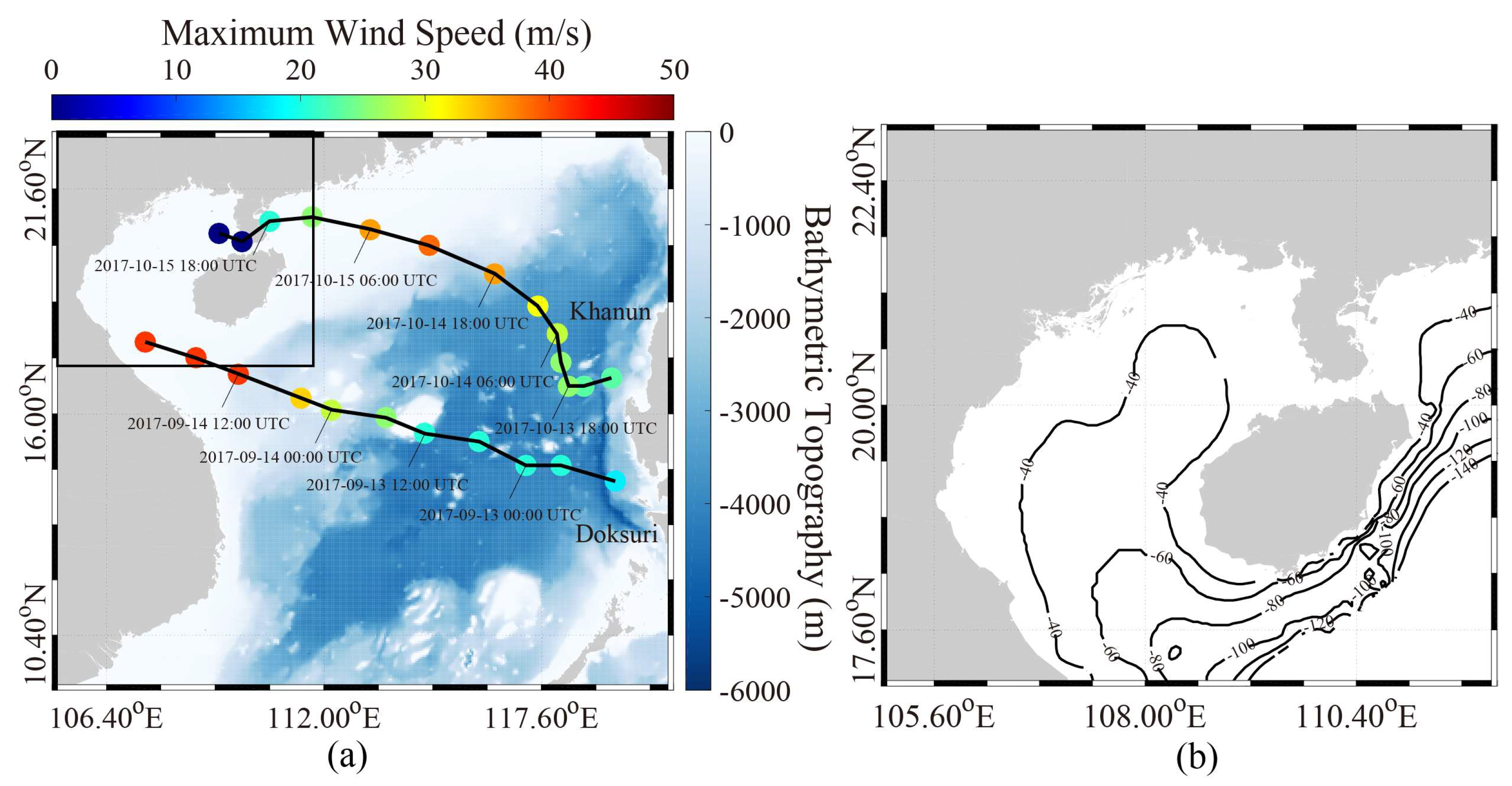
We collected tropical cyclone information in the Northwestern Pacific from the Regional Specialized Meteorological Centre (RSMC), Tokyo-Typhoon Center of Japan Meteorological Agency (JMA). Two typhoons, Doksuri and Khanun, passed through the Beibu Gulf from 12 September 2017 to 16 September 2017 and 12 October 2017 to 16 October 2017. The tracks and maximum wind speeds of the two typhoons associated with the bathymetric topography of the South China Sea are shown in Figure 1a. It is necessary to establish that these two typhoons entered the Beibu Gulf from two paths: Typhoon Khanun moving towards the Beibu Gulf through the Qiongzhou Strait (northeast) and Typhoon Doksuri passing the Beibu Gulf across the open waters of the South China Sea (southeast). Figure 1b shows the bathymetric topography of the Beibu Gulf, which is marked as a black rectangular box in Figure 1a, showing that the water depth is shallower than 50 m inside the bay.

The European Centre for Medium-Range Weather Forecasts (ECMWF) has continuously provided global gridded atmosphere-marine reanalysis data with a fine resolution of up to 0.125° × 0.125° at intervals of six hours each day since 1979. The winds and wave parameters, e.g., wind speed, wind direction, significant wave height (SWH) and mean wave period can be openly accessed from public datasets. ECMWF operational data are widely used for regional oceanography research [21,22], in particular, ECMWF wind and wave data are considered to be a reliable source in the development of wind [23,24] and wave [25] retrieval algorithms for synthetic aperture radar (SAR). However, ECMWF wave data are not applicable for wave distribution analysis because individual wind-sea and swell are absent in the datasets.

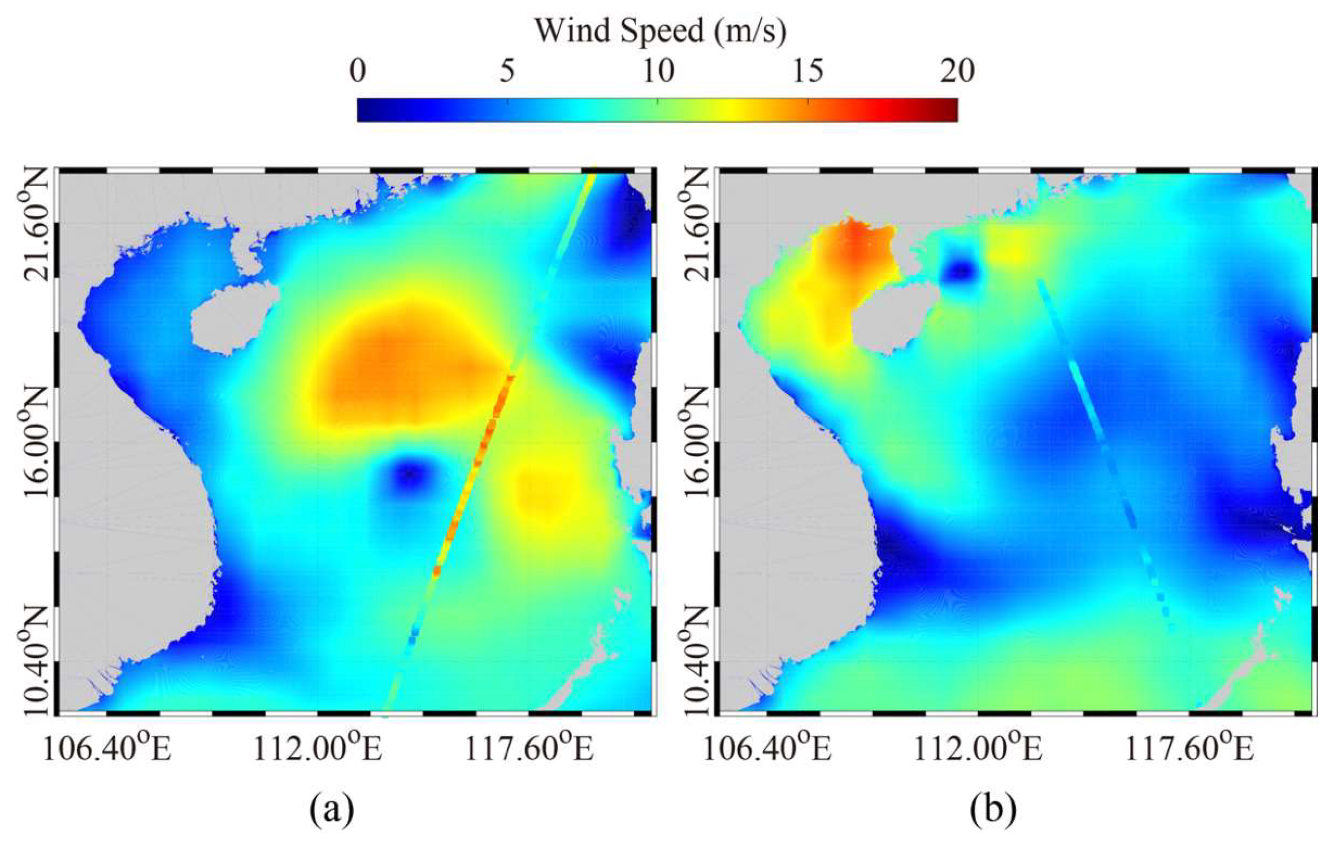
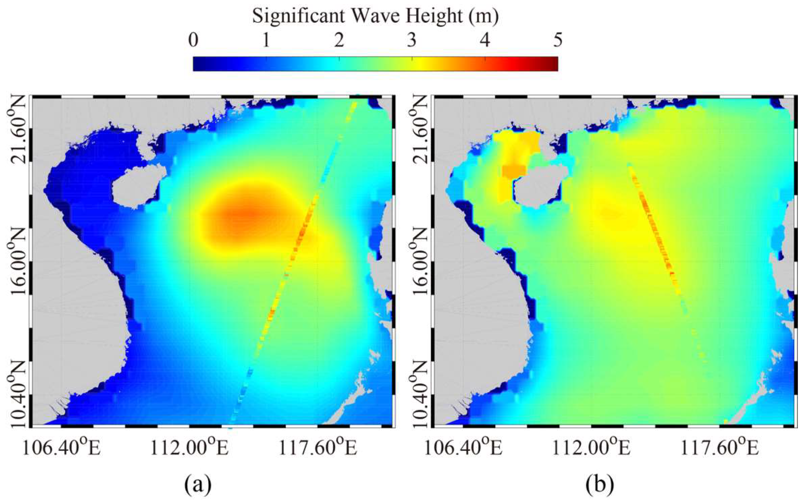
Therefore, in our study, the WW3 model is employed to simulate the wave parameters including total SWH, wind-sea SWH and swell SWH. The simulated area is the South China Sea (9° N–23° N, 105° E–121° E) and the bathymetric topography with 30 arc-second intervals (~1 km horizontal resolution) from the General Bathymetry Chart of the Oceans (GEBCO) [26] is used. The model ran from 1 September 2017 at 12:00 a.m. UTC to 1 November 2017 at 12:00 a.m. UTC. ECMWF winds are taken as the forcing wind field and ECMWF waves are employed to evaluate the accuracy of simulations. Moreover, measurements from altimeter Jason-2 are an independent source in order to validate the simulations because altimeter wave data is also applicable for regional research at basin-scale [27] and there are no available open-access moored buoys there. The time difference between simulations of the WW3 model and Jason-2 is within 15-min, as the output of WW3 is set at 30-min. As examples of the datasets, Figure 2 shows the ECMWF wind speed, overlaid by the footprints from altimeter Jason-2 during Typhoon Doksuri on 13 September 2017 at 12:00 p.m. UTC and Typhoon Khanun on 15 October 2017 at 6:00 p.m. UTC. ECMWF SWH maps overlaid with Jason-2 footprints are shown in Figure 3. Generally, although there are a few time differences between ECMWF interval data and Jason-2 footprints, both of these are roughly consistent.

3. Four Optional Packages of Nonlinear Terms and Model Setup

The WW3 model gives a unique solution of nonlinear triad wave–wave interactions and it is not exhibited here. Interestingly, the WW3 model also provides three packages for dealing with the nonlinear term for the quadruplet wave–wave interactions in the latest version 5.16, including DIA, WRT and GMDs. The details of these are briefly introduced in this section.

3.1. DIA Package

The parameterization solution of nonlinear wave–wave interactions in the wave propagation function at deep waters was initially exhibited in the study proposed in [28], named the DIA package herein. It divides nonlinear interactions into quadruplets from wavenumber vector k₁ to k₄. Meanwhile, k₁ and k₂ are assumed to be equal. Quadruplets should be satisfied with resonance conditions as follows:

$$\begin{array}{c}{\mathbf{k}}_{\mathbf{1}}+{\mathbf{k}}_{\mathbf{2}}={\mathbf{k}}_{\mathbf{3}}+{\mathbf{k}}_{\mathbf{4}}\\ {\mathsf{\sigma }}_2={\mathsf{\sigma }}_1\\ \begin{array}{c}{\mathsf{\sigma }}_3=\left({1+\mathsf{\lambda }}_{\mathrm{nl}}\right){\mathsf{\sigma }}_1\\ {\mathsf{\sigma }}_4=\left({1-\mathsf{\lambda }}_{\mathrm{nl}}\right){\mathsf{\sigma }}_1\end{array}\end{array}\},$$

(6)

in which ${\mathsf{\lambda }}_{\mathrm{nl}}=0.25$ is a constant and the relative frequency ${\mathsf{\sigma }}_1$ to ${\mathsf{\sigma }}_4$ corresponds to wavenumber vector k₁ to k₄, respectively. For each discrete wave frequency f_r and direction θ combination of the spectrum F(f_r,θ) corresponding to k₁, the contribution δS_nl to the interaction is calculated as follows:

$$\left(\begin{array}{c}{\mathsf{\delta }\mathrm{S}}_{\mathrm{nl},1}\\ {\mathsf{\delta }\mathrm{S}}_{\mathrm{nl},3}\\ {\mathsf{\delta }\mathrm{S}}_{\mathrm{nl},4}\end{array}\right)=\mathrm{D}\left(\begin{array}{c}-2\\ 1\\ 1\end{array}\right){\mathrm{Cg}}^{-4}{\mathrm{f}}_{\mathrm{r},1}^{11}\text{×}\left[{\mathrm{F}}_1^2\left(\frac{{\mathrm{F}}_3}{{\left({1+\mathsf{\lambda }}_{\mathrm{nl}}\right)}^4}+\frac{{\mathrm{F}}_4}{{\left({1-\mathsf{\lambda }}_{\mathrm{nl}}\right)}^4}\right)-\frac{{2\mathrm{F}}_1{\mathrm{F}}_3{\mathrm{F}}_4}{{\left({1-\mathsf{\lambda }}_{\mathrm{nl}}{}^2\right)}^4}\right],$$

(7)

$$\mathrm{D}=1+\frac{{\mathrm{c}}_1}{\overline{\mathrm{k}}\mathrm{d}}\left[{1-\mathrm{c}}_2\overline{\mathrm{k}}\mathrm{d}\right]{\mathrm{e}}^{{-\mathrm{c}}_3\overline{\mathrm{k}}\mathrm{d}},$$

(8)

in which, F₁ = F(f_r,1, θ), F(f_r,2, θ), etc., δS_nl,1 = δS_nl(f_r,1, θ), C = 1.0×10⁷ is taken as a proportionality constant. Equation (7) is scaled by factor D for deep water or shallow water, c₁ = 5.5, c₂ = 5/6 and c₃ = 1.25 are constants [29].

3.2. WRT Package

The WRT package exploits the Webb–Resio–Tracy method. It is based on the six-dimensional Boltzmann integral formulation and additional considerations proposed in [28,30,31,32,33,34]. The difference between the WRT and the DIA package is that the Boltzmann integral method represents the rate of change of action density of a particular wavenumber caused by resonant wave–wave interactions. The wavenumber vectors k₁ to k₄ should satisfy the resonance conditions as follows:

$$\begin{array}{c}{\mathbf{k}}_{\mathbf{1}}{+\mathbf{k}}_{\mathbf{2}}{=\mathbf{k}}_{\mathbf{3}}{+\mathbf{k}}_{\mathbf{4}}\\ {\mathsf{\sigma }}_1{+\mathsf{\sigma }}_2{=\mathsf{\sigma }}_3{+\mathsf{\sigma }}_4\end{array}\}.$$

(9)

Corresponding to wavenumber vector k₁, the rate of change of action density N₁ is given as follows:

$$\frac{\partial {\mathrm{N}}_1}{\partial \mathrm{t}}=\iiint \begin{array}{c}\mathrm{G}\left({\mathbf{k}}_{\mathbf{1}}{,\mathbf{k}}_{\mathbf{2}}{,\mathbf{k}}_{\mathbf{3}}{,\mathbf{k}}_{\mathbf{4}}\right)\mathsf{\delta }\left({\mathbf{k}}_{\mathbf{1}}{+\mathbf{k}}_{\mathbf{2}}{-\mathbf{k}}_{\mathbf{3}}{-\mathbf{k}}_{\mathbf{4}}\right)\mathsf{\delta }\left({\mathsf{\sigma }}_1{+\mathsf{\sigma }}_2{-\mathsf{\sigma }}_3{-\mathsf{\sigma }}_4\right)\\ \times \left[{\mathrm{N}}_1{\mathrm{N}}_3\left({\mathrm{N}}_4{-\mathrm{N}}_2\right){+\mathrm{N}}_2{\mathrm{N}}_4\left({\mathrm{N}}_3{-\mathrm{N}}_1\right)\right]\end{array}{\mathrm{d}\mathbf{k}}_{\mathbf{2}}{\mathrm{d}\mathbf{k}}_{\mathbf{3}}{\mathrm{d}\mathbf{k}}_{\mathbf{4}},$$

(10)

in which each action density N is determined by the wavenumber vectors k. The term G is a complicated coefficient given in [35], and the delta function is removed by many transformations.

An important step in the WRT package is taking a space integral for each (k₁, k₃) combination, as exhibited,

$$\frac{\partial {\mathrm{N}}_1}{\partial \mathrm{t}}=2\int {\mathrm{T}(\mathbf{k}}_{\mathbf{1}}{,\mathbf{k}}_{\mathbf{3}}{)\mathrm{d}\mathbf{k}}_{\mathbf{3}},$$

(11)

$$\mathrm{T}=\iint \begin{array}{c}\mathrm{G}\left({\mathbf{k}}_{\mathbf{1}}{,\mathbf{k}}_{\mathbf{2}}{,\mathbf{k}}_{\mathbf{3}}{,\mathbf{k}}_{\mathbf{4}}\right)\mathsf{\delta }\left({\mathbf{k}}_{\mathbf{1}}{+\mathbf{k}}_{\mathbf{2}}{-\mathbf{k}}_{\mathbf{3}}{-\mathbf{k}}_{\mathbf{4}}\right)\\ \times \mathsf{\delta }\left({\mathsf{\sigma }}_1{+\mathsf{\sigma }}_2{-\mathsf{\sigma }}_3{-\mathsf{\sigma }}_4\right)\mathsf{\theta }\left({\mathbf{k}}_{\mathbf{1}}{,\mathbf{k}}_{\mathbf{3}}{,\mathbf{k}}_{\mathbf{4}}\right)\\ \times \left[{\mathrm{N}}_1{\mathrm{N}}_3\left({\mathrm{N}}_4{-\mathrm{N}}_2\right){+\mathrm{N}}_2{\mathrm{N}}_4\left({\mathrm{N}}_3{-\mathrm{N}}_1\right)\right]\end{array}{\mathrm{d}\mathbf{k}}_{\mathbf{2}}{\mathrm{d}\mathbf{k}}_{\mathbf{4}},$$

(12)

$$\mathsf{\theta }\left({\mathbf{k}}_{\mathbf{1}}{,\mathbf{k}}_{\mathbf{3}}{,\mathbf{k}}_{\mathbf{4}}\right)=\{\begin{array}{c}1,\left|{\mathbf{k}}_{\mathbf{1}}{-\mathbf{k}}_{\mathbf{3}}\right|\le \left|{\mathbf{k}}_{\mathbf{1}}{-\mathbf{k}}_{\mathbf{4}}\right|\\ 0,\left|{\mathbf{k}}_{\mathbf{1}}{-\mathbf{k}}_{\mathbf{3}}\right|\text{>}\left|{\mathbf{k}}_{\mathbf{1}}{-\mathbf{k}}_{\mathbf{4}}\right|\end{array}.$$

(13)

Compared with the DIA package, the computation of the WRT package is much larger, and more accurate. Therefore, the WRT package a powerful capability for highly-idealized case, as mentioned in technical document of WW3 model [29].

3.3. GMD Package

The GMD package is an extension of the DIA package. It has been developed in three ways as follows:

• The definition of quadruplets is expanded.
• The equations mentioned in Section 3.1 are improved for arbitrary depths, even at extremely shallow waters, e.g., Beibu Gulf where the water depth is shallower than 5 m.
• The use of multiple quadruplets is introduced.

The resonance conditions of the GMD package are expanded as

$$\begin{array}{c}{\mathsf{\sigma }}_1{=\mathrm{a}}_1{\mathsf{\sigma }}_{\mathrm{r}}\\ {\mathsf{\sigma }}_2{=\mathrm{a}}_2{\mathsf{\sigma }}_{\mathrm{r}}\\ \begin{array}{c}{\mathsf{\sigma }}_3{=\mathrm{a}}_3{\mathsf{\sigma }}_{\mathrm{r}}\\ \begin{array}{c}{\mathsf{\sigma }}_4{=\mathrm{a}}_4{\mathsf{\sigma }}_{\mathrm{r}}\\ {\mathsf{\theta }}_{12}{=\mathsf{\theta }}_1{\text{±}\mathsf{\theta }}_{12}\end{array}\end{array}\end{array}\},$$

(14)

where a₁ + a₂ = a₃ + a₄ is satisfied by the general resonance conditions, σ_r is a reference frequency and θ₁₂ is an angular difference between the wavenumber k₁ and k₂. The other parameters are tuned parameters, named one-parameter (λ), two-parameter (λ,μ), or three-parameter (λ,μ,θ₁₂) quadruplet, in which λ and μ are the constants.

In the GMD package, a two-component scaling function, named the deep scaling function and the shallow scaling function, is proposed for calculating arbitrary depths. Then, Equation 7 of the DIA package is transformed to:

$$\left(\begin{array}{c}{\mathsf{\delta }\mathrm{S}}_{\mathrm{nl},1}\\ {\mathsf{\delta }\mathrm{S}}_{\mathrm{nl},2}\\ \begin{array}{c}{\mathsf{\delta }\mathrm{S}}_{\mathrm{nl},3}\\ {\mathsf{\delta }\mathrm{S}}_{\mathrm{nl},4}\end{array}\end{array}\right)\left(\begin{array}{c}-1\\ -1\\ \begin{array}{c}1\\ 1\end{array}\end{array}\right)(\frac{1}{{\mathrm{n}}_{\mathrm{q},\mathrm{d}}}{\mathrm{C}}_{\mathrm{deep}}{\mathrm{B}}_{\mathrm{deep}}+\frac{1}{{\mathrm{n}}_{\mathrm{q},\mathrm{s}}}{\mathrm{C}}_{\mathrm{shal}}{\mathrm{B}}_{\mathrm{shal}})\times [\frac{{\mathrm{c}}_{\mathrm{g},1}{\mathrm{F}}_1}{{\mathrm{k}}_1{\mathsf{\sigma }}_1}\frac{{\mathrm{c}}_{\mathrm{g},2}{\mathrm{F}}_2}{{\mathrm{k}}_2{\mathsf{\sigma }}_2}\left(\frac{{\mathrm{c}}_{\mathrm{g},3}{\mathrm{F}}_3}{{\mathrm{k}}_3{\mathsf{\sigma }}_3}+\frac{{\mathrm{c}}_{\mathrm{g},4}{\mathrm{F}}_4}{{\mathrm{k}}_4{\mathsf{\sigma }}_4}\right)-\frac{{\mathrm{c}}_{\mathrm{g},3}{\mathrm{F}}_3}{{\mathrm{k}}_3{\mathsf{\sigma }}_3}\frac{{\mathrm{c}}_{\mathrm{g},4}{\mathrm{F}}_4}{{\mathrm{k}}_4{\mathsf{\sigma }}_4}\left(\frac{{\mathrm{c}}_{\mathrm{g},1}{\mathrm{F}}_1}{{\mathrm{k}}_1{\mathsf{\sigma }}_1}+\frac{{\mathrm{c}}_{\mathrm{g},2}{\mathrm{F}}_2}{{\mathrm{k}}_2{\mathsf{\sigma }}_2}\right)],$$

(15)

$${\mathrm{B}}_{\mathrm{deep}}=\frac{{\mathrm{k}}^{4+\mathrm{m}}{\mathsf{\sigma }}^{13-2\mathrm{m}}}{{\left(2\mathsf{\pi }\right)}^{11}{\mathrm{g}}^{4—\mathrm{m}}{\mathrm{c}}_{\mathrm{g}}^2},$$

(16)

$${\mathrm{B}}_{\mathrm{shal}}=\frac{{\mathrm{g}}^2{\mathrm{k}}^{11}}{{\left(2\mathsf{\pi }\right)}^{11}{\mathrm{c}}_{\mathrm{g}}}{\left(\mathrm{kd}\right)}^{\mathrm{n}}$$

(17)

in which, B_deep and B_shal are the deep and shallow scaling functions with tuned parameters m and n, n_q,d and n_q,s are the number of quadruplets, and C_deep and C_shal are the corresponding deep and shallow water tuned constants.

Compared to the DIA package, the GMD package has four quadruplets and each quadruplet has four times the computational power of the DIA package. There are two kinds of coefficients in the application of the GMD package, herein called GMD1 and GMD2 [29] for convenience. GMD1 and GMD2 represents three-parameter and the five-parameter parametrization, respectively. The tuned parameters n_q, m, n, λ, μ, θ₁₂, C_deep and C_shal are shown in

Table 1. The tuned parameters used in this study when Generalized Multiple DIA (GMD) packages are implemented.

Package Name	nq	m	n	λ	μ	θ12	Cdeep	Cshal
GMD1	3	0.00	−3.5	0.126	0.00	−1.0	4.790 × 107	0.00
				0.237	0.00	−1.0	2.200 × 107	0.00
				0.319	0.00	−1.0	1.110 × 107	0.00
GMD2	5	0.00	−3.5	0.066	0.018	21.4	0.170 × 109	0.00
				0.127	0.069	19.6	0.127 × 109	0.00
				0.228	0.065	2.0	0.443 × 108	0.00
				0.295	0.196	40.5	0.210 × 108	0.00
				0.369	0.226	11.5	0.118 × 108	0.00

.

3.4. Model Setup

In our study, ECMWF winds at 0.125° grids are the forcing field, which has a coarser spatial resolution than bathymetric data from 30 arc-second GEBCO. The open boundary with 0.5° grids is forced by wave simulations from the WW3 model at a longitude of 100–125°E and latitude of 5–25°N, in which the ECMWF winds and GEBCO bathymetric data is bilinear interpolated to be 0.5° grids. The simulated two-dimensional wave spectrum is default resolved into 24 regular azimuthal directions and the frequency bins are logarithmically ranged from 0.04118 to 0.7186 at an interval of Δf/f = 0.1. The time step of spatial propagation is set to 300 s in both the longitude and latitude directions. In order to obtain reasonable simulations, the outputs are set as a spatial grid of 0.2°, due to the ECMWF winds and GEBCO bathymetric data is determined to be 0.2° grids here.

4. Results

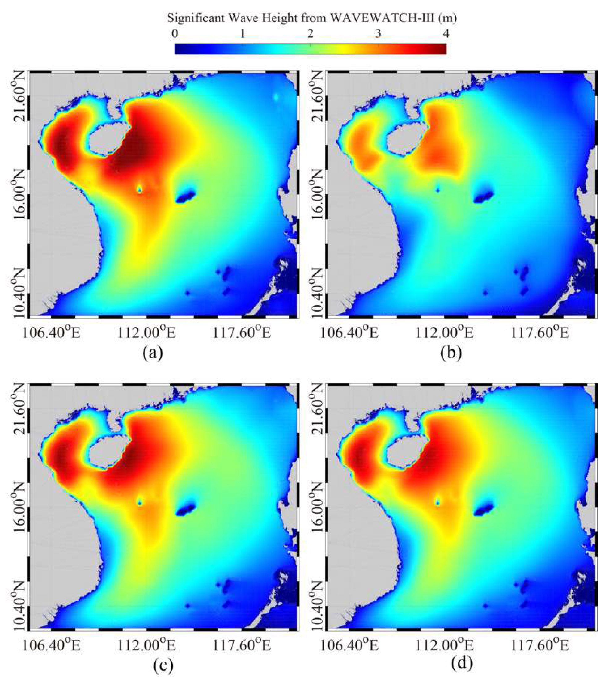
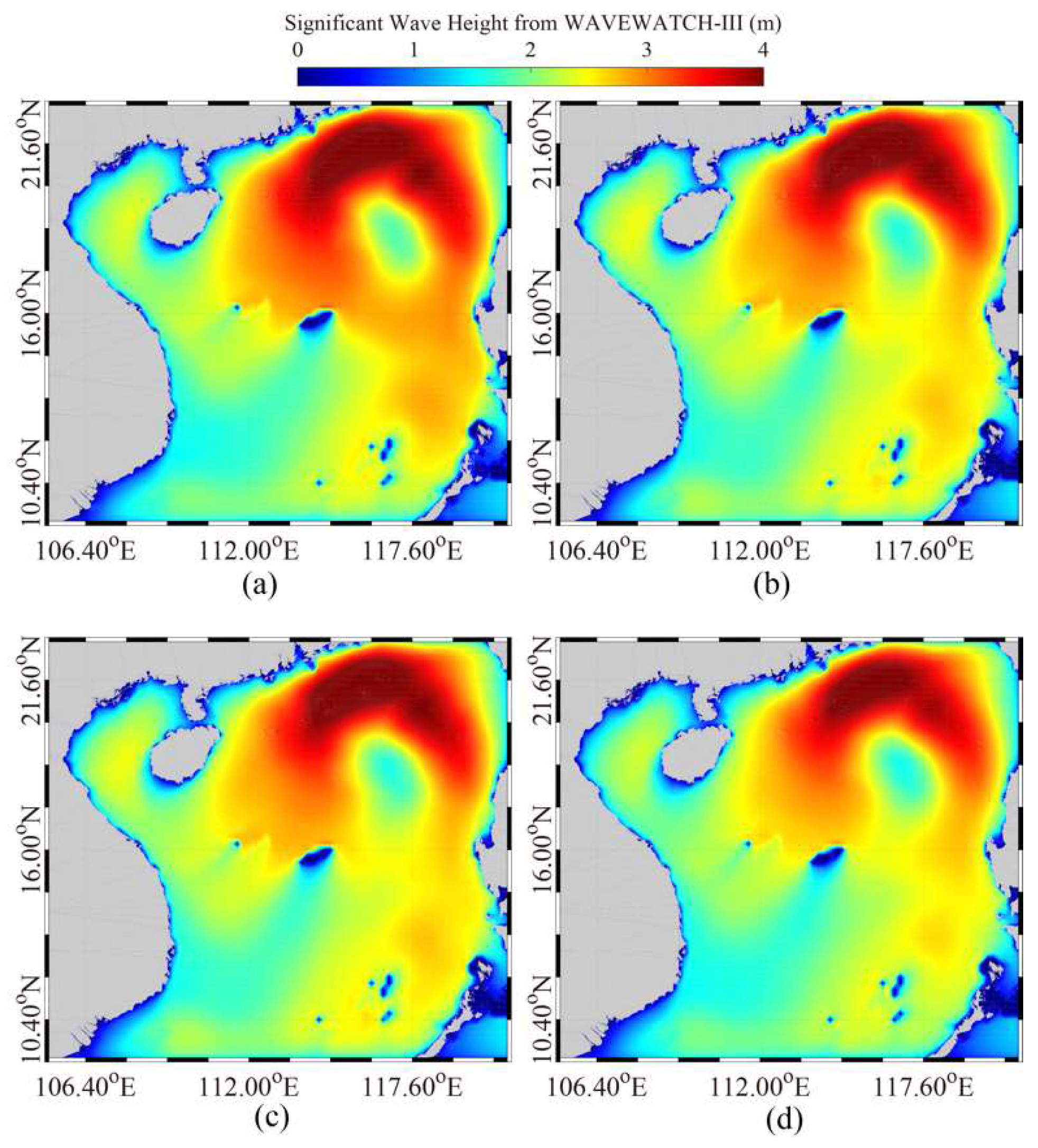
We simulated typhoon-induced waves using the WW3 model from 1 September 2017 at 12:00 a.m. UTC to 1 November 2017 at 12:00 a.m. UTC. The total SWH simulations at 12:00 a.m. UTC on 15 September 2017 and at 12:00 a.m. UTC on 15 October 2017 when typhoons Doksuri and Khanun passed the Beibu Gulf, are shown as examples in Figure 4 and Figure 5, in which a–d represent the results using DIA, WRT, GMD1 and GMD2, respectively. It is found that the maximum SWH is nearly 4 m, and the simulated SWH using the WRT package is obviously smaller than the results using other packages, especially around Hainan island for Typhoon Doksuri. It is not surprising, as the WRT package works better for a highly-idealized case, while the water depth and bottom slope significantly change near the island. To further study the accuracy of those packages with nonlinear terms for quadruplets wave–wave interactions, the simulations are compared with SWH from ECMWF and Jason-2.

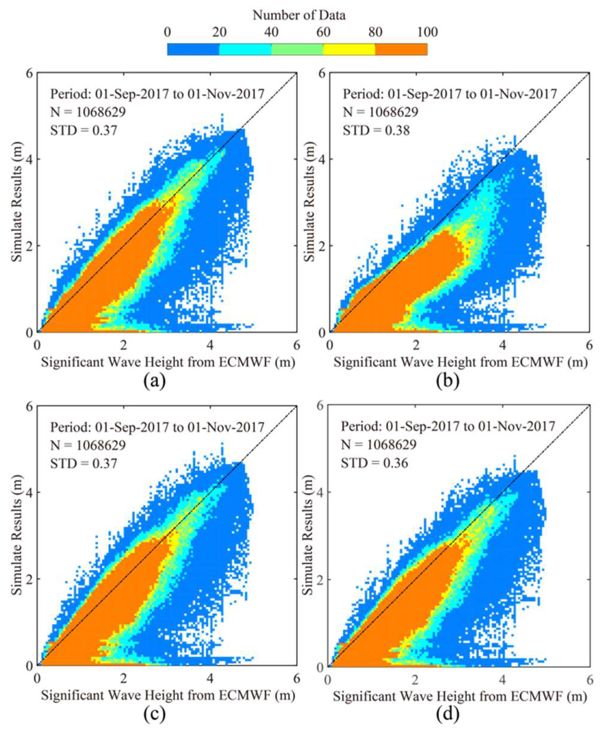
The simulations closest to the ECMWF grid data were chosen. The comparisons between simulation results and SWH from ECMWF during the period from 1 September 2017 to 1 November 2017 are shown in Figure 6. The standard deviation (STD) of SWH using the DIA and GMD1 packages is 0.37 m as shown in Figure 6a and Figure 6c. A slightly larger 0.38 m STD of the SWH is presented in Figure 6b using the WRT package and the simulated SWH is smaller than the ECMWF-based result, especially for SWHs greater than 2 m. A 0.36 STD is achieved in Figure 6d when using GMD2. It not surprising that the simulated results have a better agreement with SWH from ECMWF since it was ECMWF winds that were used as the forcing field. Therefore, an independent source is further used to validate the simulations from the WW3 model.

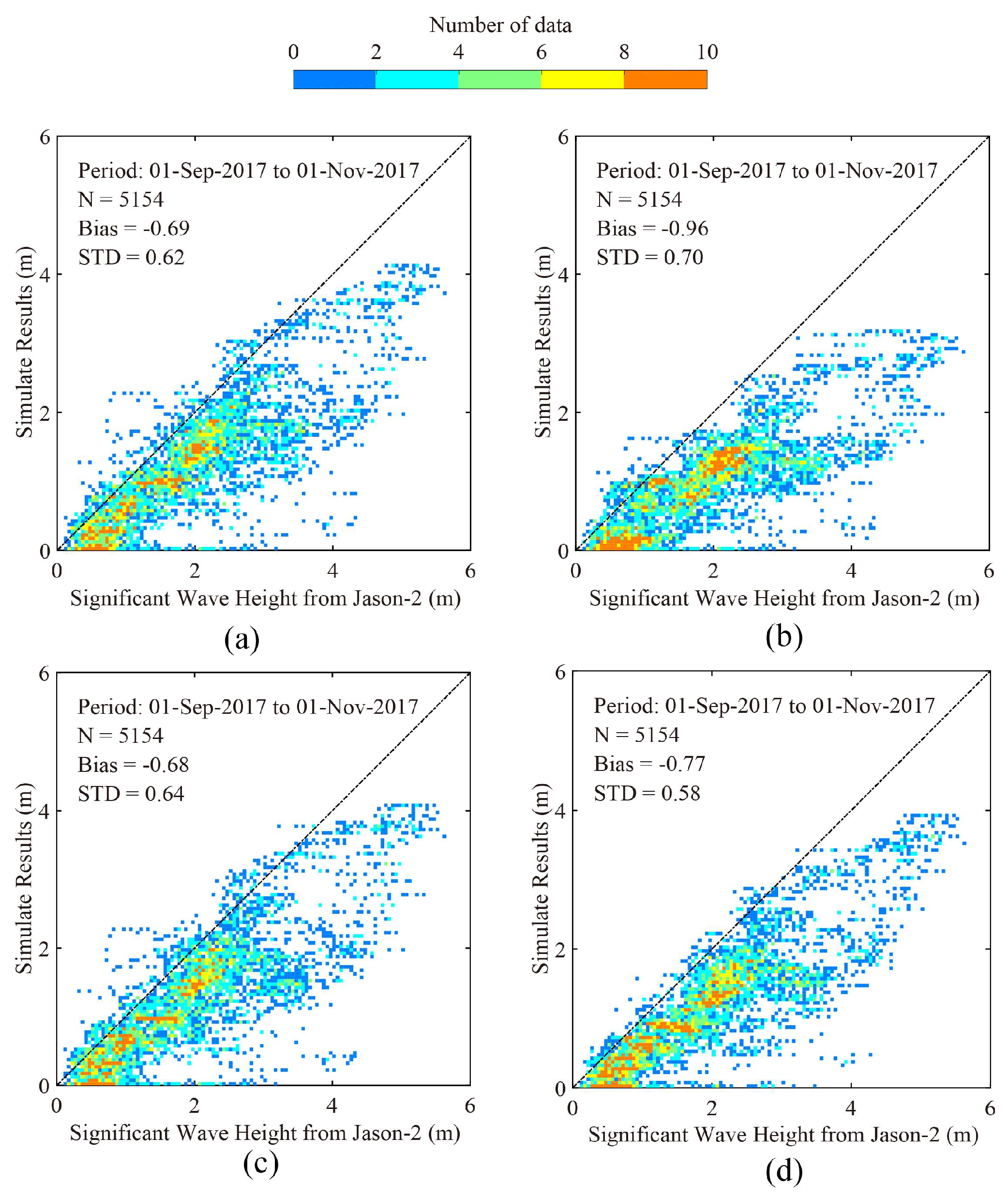
In total, we had more than 5000 matchups covering the WW3 grids during the period of the two typhoons, Doksuri and Khanun, in the South China Sea. Figure 7 shows the comparisons between SWH simulations using the optional packages and SWH measured from altimeter Jason-2. Simulated SWH is generally underestimated as shown by the results validated against altimeter Jason-2. Moreover, the simulated SWH using the WRT package is also obviously smaller than the altimeter-measured SWH at SWHs greater than 2 m. This result is consistent with the conclusion in [36] that ECMWF data generally underestimate the wind speed and SWH compared with in situ buoys and altimeter measurements. A 0.62 m STD, 0.64 m STD and 0.58 m STD of SWH using the DIA, GMD1 and GMD2 packages were achieved and these are shown in Figure 7a, Figure 7c and Figure 7d, respectively. A larger 0.70 m STD of SWH using the WRT package is shown in Figure 7b. Collectively, the WRT package may not be suitable for wave simulation in complicated bathymetric topography and extreme conditions.

5. Discussion

Although the DIA package is suitable for wave simulations at deep or shallow waters as the factor D can be adopted according to the local water depth, the key point of the GMD package is the use of multiple quadruplets, indicating its more powerful capability for use in complex topography regions. Although the GMDs have the same formulation, GMD2 has a better performance than GMD1 according to the above statistical analysis. The calculations of the WRT package are more accurate and the computations are larger than in other packages. However, it requires a regular underwater topography, e.g., triangular gridded and sub-grid information. This is a probable explanation that the WRT package has a large deviation compared with other packages. As a result, the simulations from the WW3 model using the GMD2 package were employed to analyze the wave characteristics in the Beibu Gulf during the period of the two typhoons. It is concluded in [36] that ECMWF wave data has good homogeneity over global seas, and therefore has a great advantage for the estimation of wave height trends. In this study, the error between the simulated results from the WW3 model and SWH from ECMWF is less than 0.40 m, indicating that the simulations are suitable for analyzing the wave distribution here.

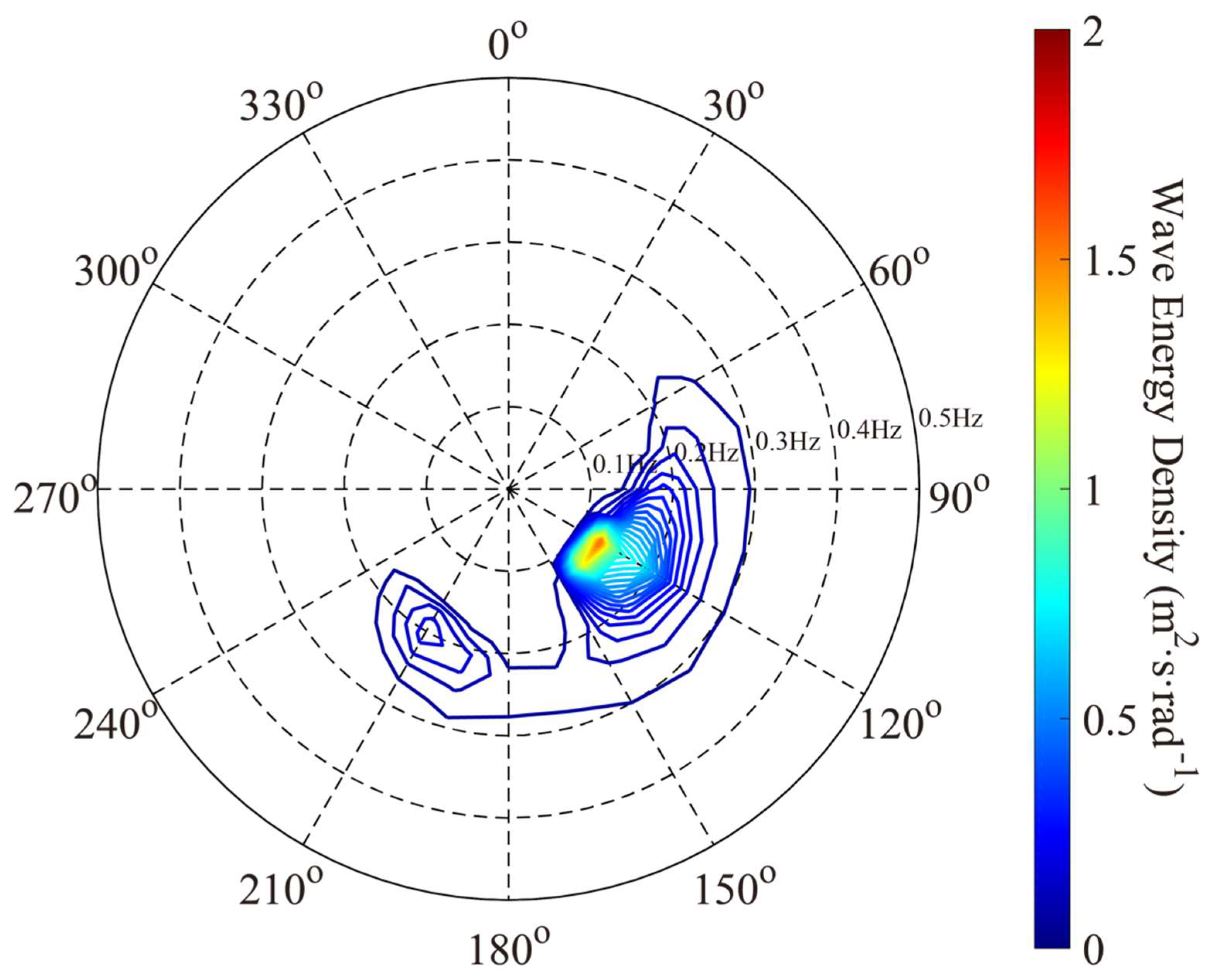
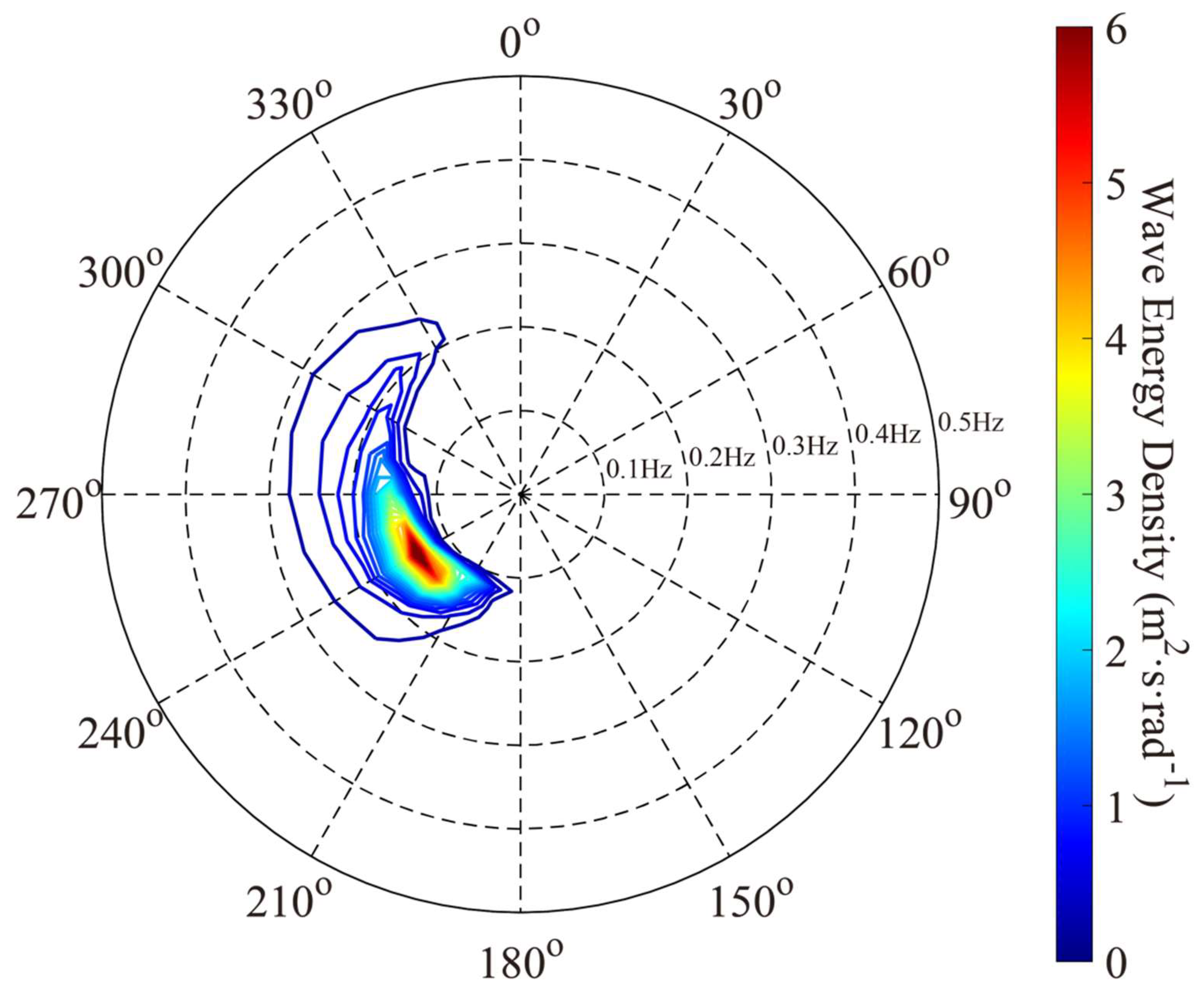
In this study, the simulated wind-sea and swell from the WW3 model are separately exported using the method proposed in [37], which is widely employed to study the analysis of wind-sea [38] and swell distribution [39] over global seas using the WW3 model. As examples, the wave spectrum at the fixed point, located at the middle of the Beibu Gulf (19.5° N, 107.5° E) at the specific moments in two typhoons are presented here. The two-dimensional wave energy density simulated using the GMD2 package at 6:00 a.m. UTC on 16 September 2017 in Typhoon Doksuri and at 6:00 a.m. UTC 16 October 2017 in Typhoon Khanun, are analyzed in Figure 8 and Figure 9, respectively. At this time, swell and wind-sea are mixed for Typhoon Doksuri while wind-sea dominates for Typhoon Khanun. Interestingly, the direction of and wind-sea and swell have about a 45° deviation for Typhoon Doksuri. We think it is probably caused by wave reflection of the coastline. However, the wave direction for Typhoon Khanun is consistent with wind direction.

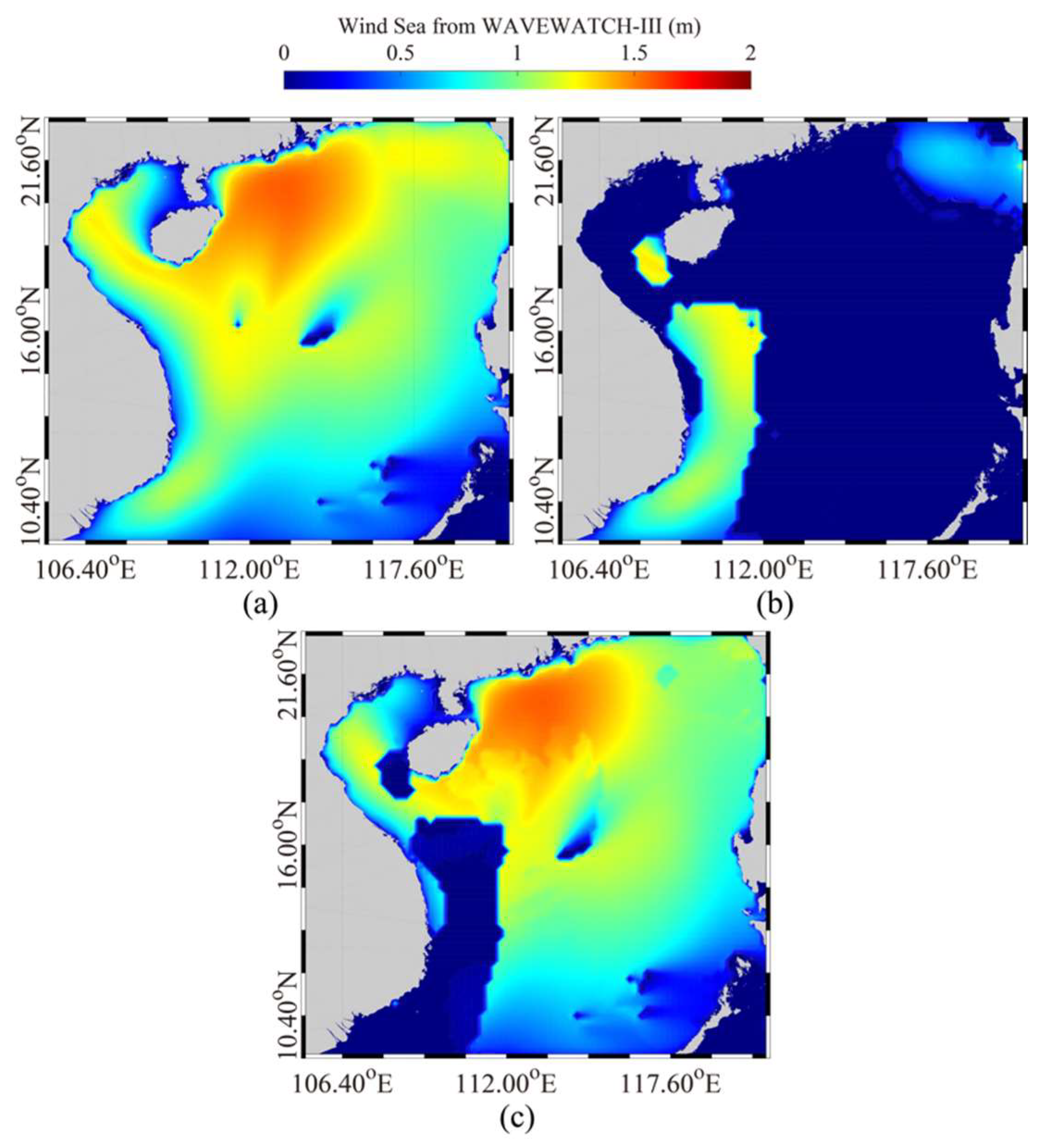
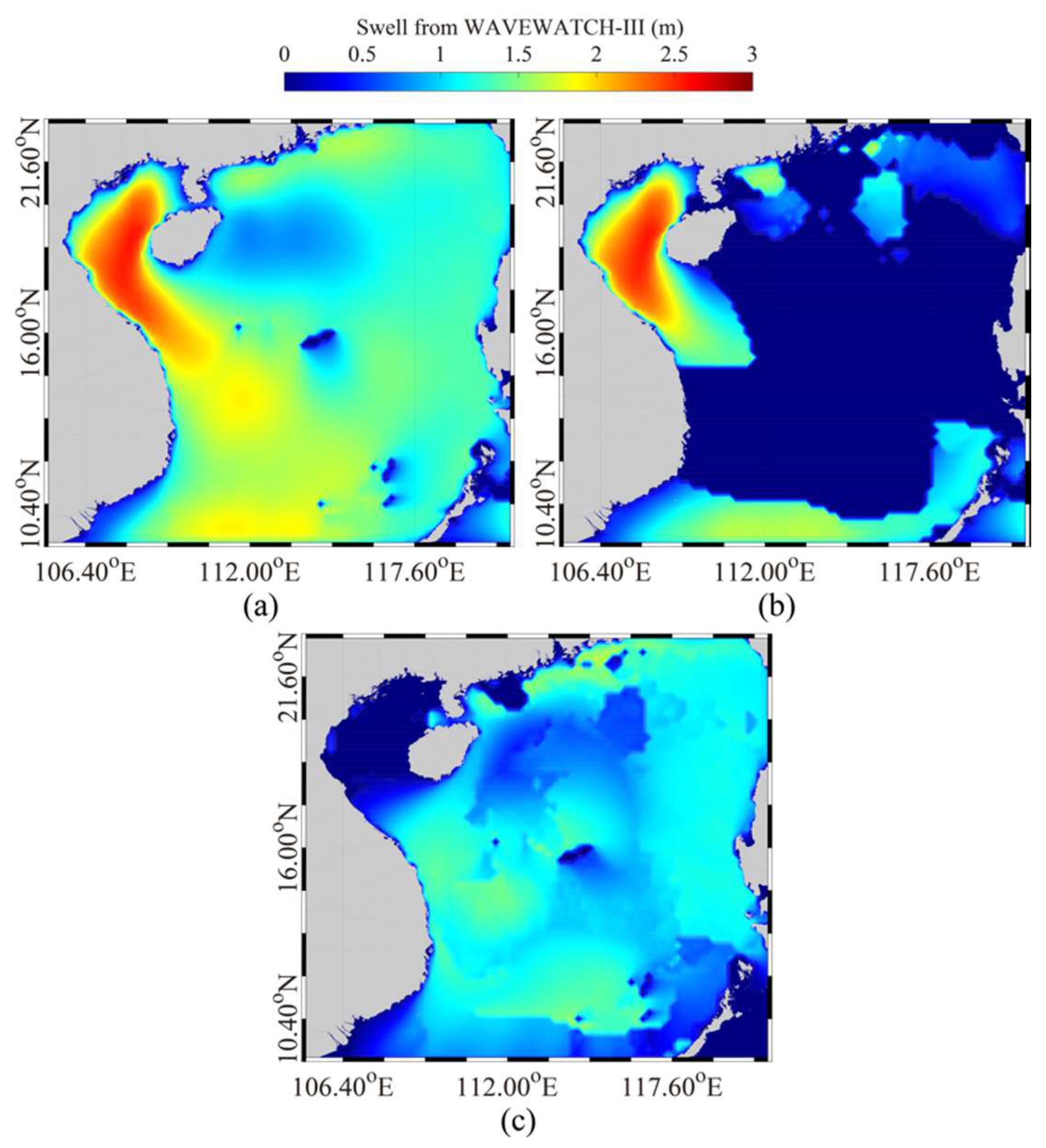
Figure 10a–c show the distribution of total SWH, wind-sea and swell, respectively, during the period of Typhoon Doksuri at 6:00 a.m. UTC on 16 September 2017 in the whole bay. The track of Typhoon Doksuri passing through the Beibu Gulf in the southeast is shown in Figure 1a. Interestingly, swell almost dominates the whole bay at this time. Similarly, Figure 11a–c show the distribution of total SWH, wind-sea and swell, respectively, during the period of Typhoon Khanun at 6:00 a.m. UTC on 16 October 2017. Opposite to Typhoon Doksuri, Typhoon Khanun passed through the Beibu Gulf in the northeast. It is observed that wind-sea almost dominates the whole bay and swell mainly contributes in the east of Hainan Island outside the Beibu Gulf. As this example shows, the wave distribution is different when the typhoons pass through the Beibu Gulf from the two paths.

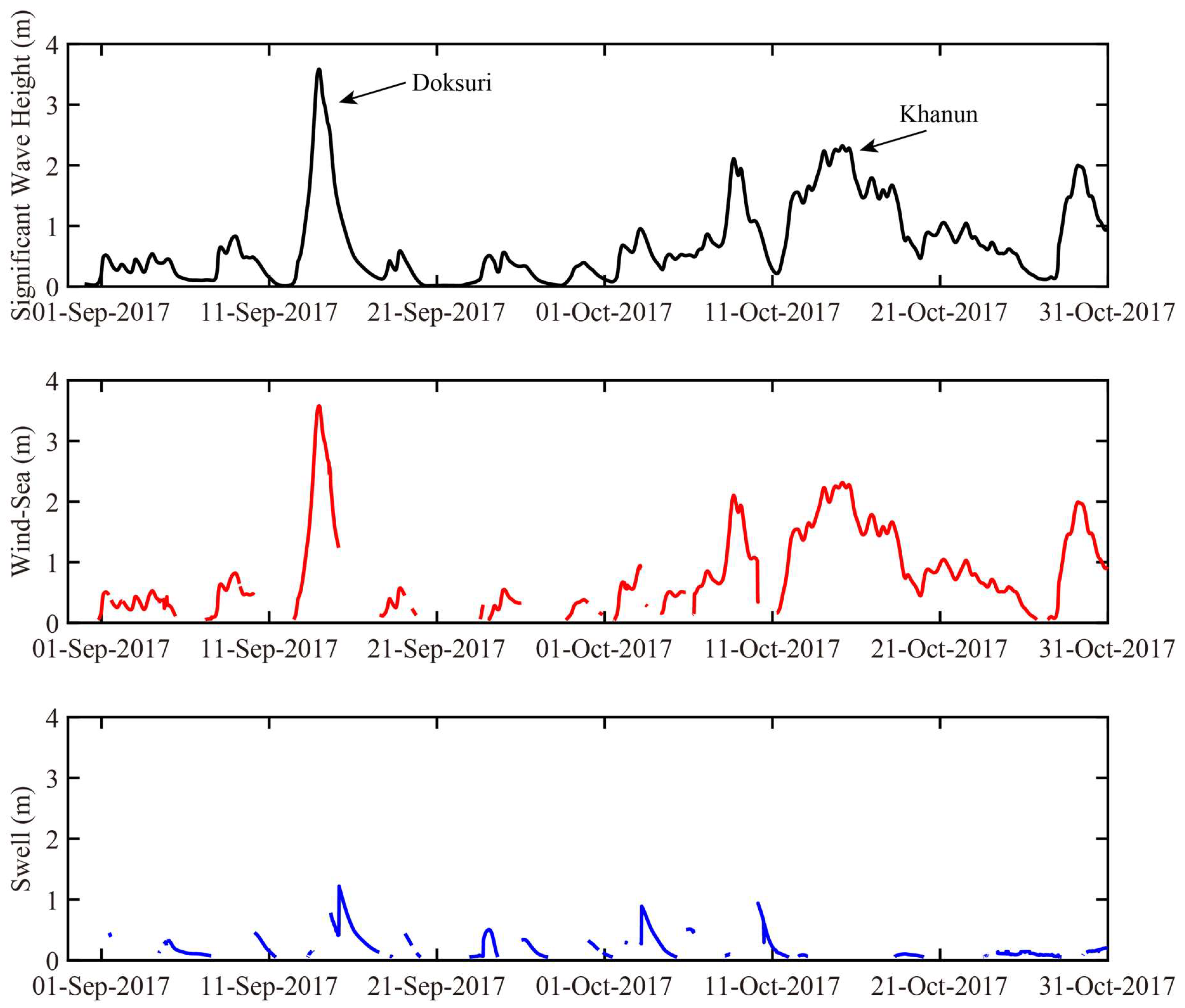
We also analyzed the wave height trend at a fixed point (19.5° N, 107.5° E) during the period from 1 September 2017 to 31 October 2017. The time series of SWH, wind-sea and swell at this point are exhibited in Figure 12. It can be clearly observed that wind-sea and swell in the Beibu Gulf are mixed during the period of typhoon Doksuri and swell dominates when the threshold of wind-sea passes. However, wind-sea state is dominant because there is little contribution from swell during the whole duration of Typhoon Khanun.

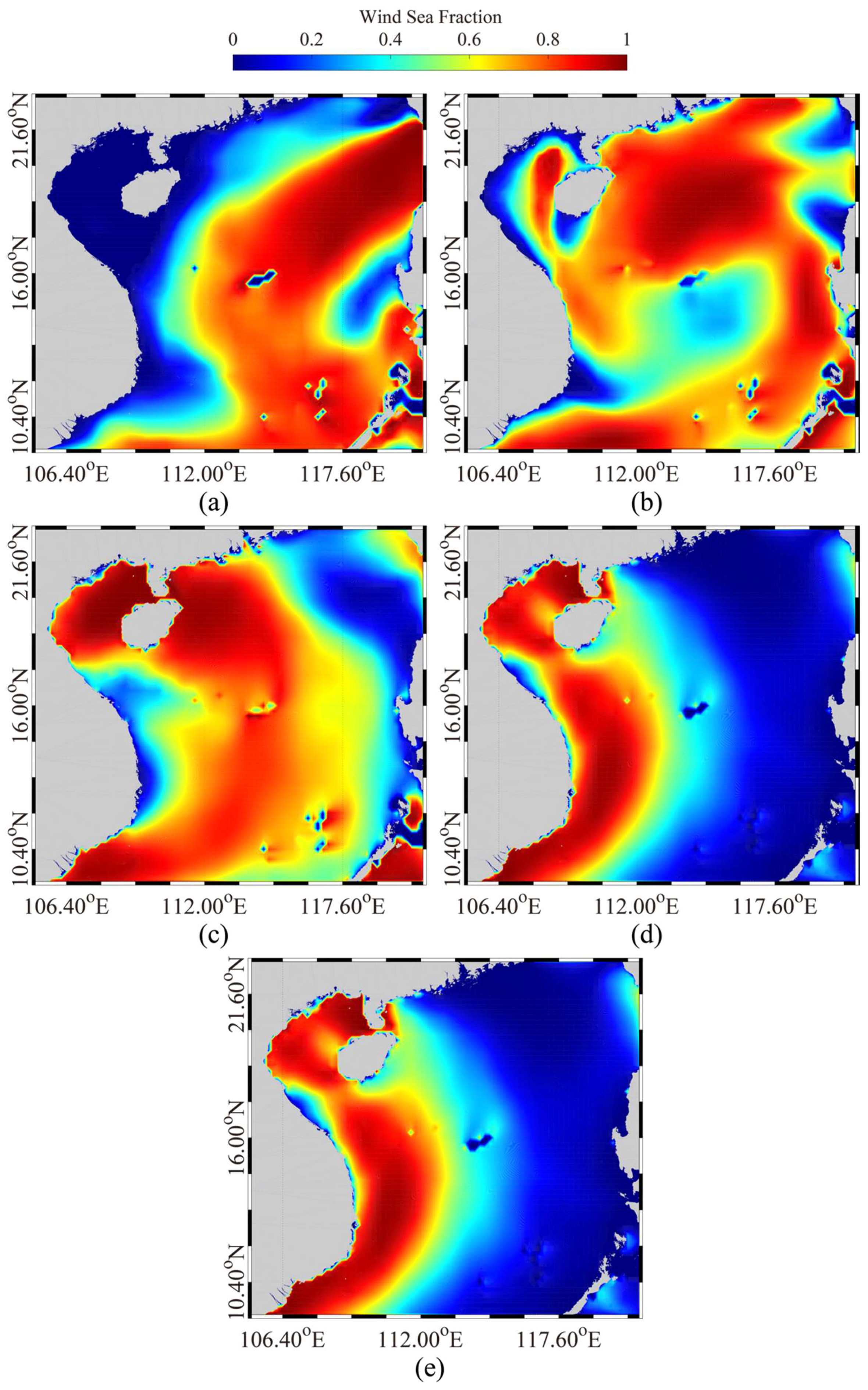
In order to further analyze the wave distribution in the Beibu Gulf, the daily mean wind-sea fraction of Typhoon Doksuri from 12 September 2017 to 17 September 2017 is presented in Figure 13. It is shown that wind-sea occurred in Beibu Bay from 13 September 2017 to 15 September 2017, while swell propagated into the Beibu Gulf after 16 September 2017. As Typhoon Doksuri enters the Beibu Gulf at the southeast, wind-sea propagates in a counter-clockwise direction along the coastline, causing wind-sea to stay and grow in Beibu Bay for a long period. This is the probable explanation for the two-day delay in swell occurrence. Interestingly, swell dominates around the Vietnamese coastal waters with the ratio of swell energy in the total up to 60% on 14 September. This behavior deserves further study through more typhoons.

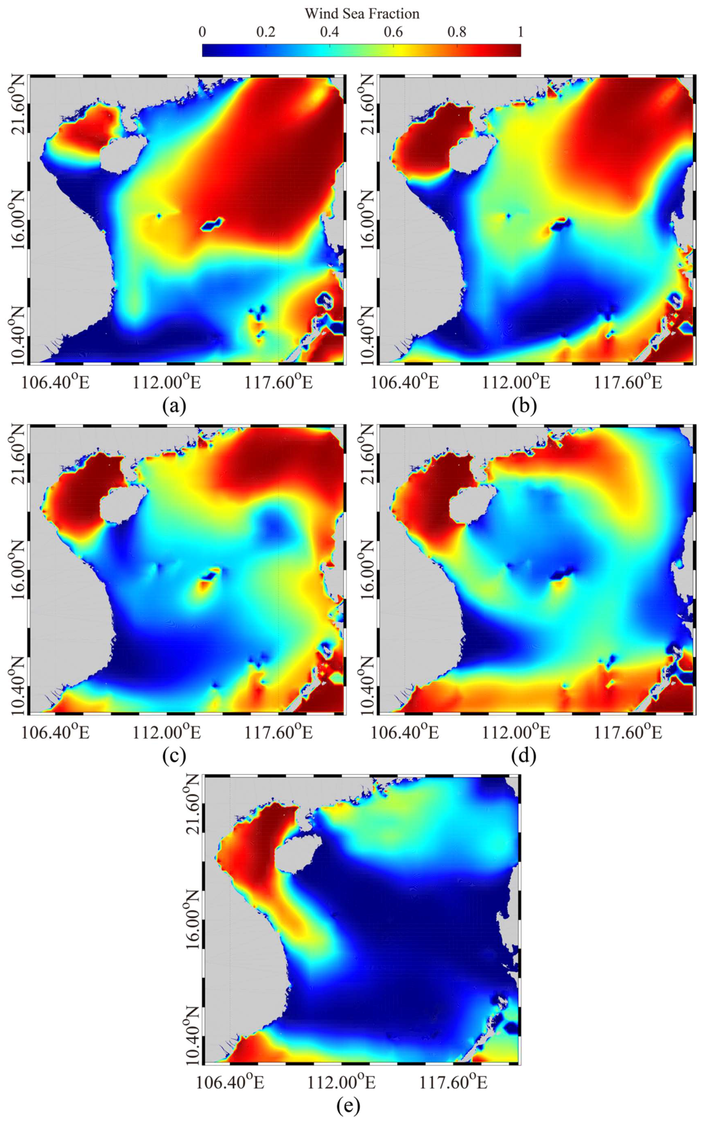
The daily mean wind-sea fraction during the period of typhoon Khanun from 12 October 2017 to 16 October 2017 is exhibited in Figure 14. Wind-sea propagates inside the Beibu Gulf on 12 October 2017; however, swell distributes in the east of Hainan Island outside the Beibu Gulf. A reasonable explanation for this is that Typhoon Khanun moves towards the Beibu Gulf in a northeasterly direction, causing wind-sea at a small scale to enter the bay through the Qiongzhou Strait while a typhoon-induced swell at mesoscale is difficult to propagate into the bay. This finding is consistent with the analysis at the fixed point.

6. Conclusions

To date, few research works have focused on the analysis of wave distribution in the South China Sea through observations [40] and model simulation [41,42]. The Beibu Gulf is a semi-enclosed bay in the South China Sea. It is an abundant fishery resource, and also subject to much human activity. In summer, typhoons from the Pacific Ocean frequently pass through the Beibu Gulf where the water depth is shallower than 50 m. In particular, there are two paths in the Gulf though which typhoons can pass. Therefore, the regional wave distribution in the Beibu Gulf is worthy of study, especially under typhoon conditions. In this work, we investigate the applicability of the latest version of the WW3 model (5.16) and analyze the typhoon-induced wave distribution in the Beibu Gulf.

Non-linear wave–wave interactions are important considerations in the wave simulation at shallow waters. The WW3 model provides four optional packages of nonlinear term for quadruplets wave–wave interactions, named DIA, WRT, GMD1 and GMD2. The wave fields (basically SWH) were simulated using these four packages from 1 September 2017 to 31 October 2017, during which time typhoons Doksuri and Khahun entered the Beibu Gulf in two paths. The simulated SWH are compared with SWH from ECMWF and measurements from altimeter Jason-2, showing simulated SWH is under-estimated using the WRT package especially for SWHs greater than 2 m. This is mainly because WRT requires highly-idealized gridded topography, e.g., triangular gridded and sub-grid information. GMDs with multiple quadruplets are an extension of DIA. Although GMDs are defined as unique formations, the accuracy of simulated SWH was improved using the GMD2 package.

Based on the simulated results from the WW3 model with the GMD2 package, the wave distribution in the Beibu Gulf during the period of typhoons Doksuri and Khahu was analyzed. It is not surprising that typhoon-induced wave distributions in the Beibu Gulf are different as the typhoons enter the bay in two separate paths. For Typhoon Doksuri passing through the Beibu Gulf in the southeast, wind-sea is dominant at the early and middle stages because wind-sea stays and grows in Beibu Bay for a long period and swell dominates at the later stage. However, wind-sea dominates throughout the whole stage as Typhoon Khanun moves through Qiongzhou Strait in the northeast. Swell distributes outside the Beibu Gulf around the east of Hainan Island because the typhoon-induced swell is difficult to propagate into the Beibu Gulf through the narrow Qiongzhou Strait and swell dominates to the east of Hainan Island outside the bay.

In summary, it is concluded that the GMD2 package of the nonlinear term for quadruplets wave–wave interactions is recommended for simulating typhoon waves in South China Sea. In the near future, we plan to simulate waves using the WW3 model under the background of typhoons, which have passed through the South China Sea over the last 30 years, and the climatology of typhoon-induced waves in the South China Sea will be analyzed.

References

- Jiang, C.B.; Zhao, B.B.; Deng, B.; Wu, Z.Y. Numerical simulation of typhoon storm surge in the Beibu Gulf and hazardous analysis at key areas. Marin Forec. 2017, 34, 32–40. (In Chinese) [Google Scholar]
- Chen, B.; Chen, X.Y.; Dong, D.X.; Shi, M.C.; Qiu, S.F. Analysis of the influence of water level change in Guangxi nearshore caused by typhoon landed in the north of Beibu Gulf. Guangxi Sci. 2015, 22, 245–249. (In Chinese) [Google Scholar]
- Zeng, W.G.; Wu, F. Risk assessment on geological disaster caused by typhoon and rainstorm in Beibu Gulf economic zone of Guangxi Zhuang autonomous region. Chin. J. Geol. Hazard Contr. 2017, 28, 121–127. (In Chinese) [Google Scholar]
- Quilfen, Y.; Tournadre, J.; Chapron, B. Altimeter dual-frequency observations of surface winds, waves, and rain rate in tropical cyclone Isabel. J. Geophys. Res. 2006, 111, C01004. [Google Scholar] [CrossRef]
- Kudryavtseva, N.A.; Soomere, T. Validation of the multi-mission altimeter wave height data for the Baltic Sea region. Est. J. Earth Sci. 2016, 65, 161–175. [Google Scholar] [CrossRef]
- Liu, Q.X.; Babanin, A.V.; Guan, C.L.; Zieger, S.; Sun, J.; Jia, Y. Calibration and validation of HY-2 altimeter wave height. J. Atmos. Ocean Technol. 2016, 33, 919–936. [Google Scholar] [CrossRef]
- The WAMDI Group. The WAM Model—A third generation ocean wave prediction model. J. Phys. Oceanogr. 1988, 18, 1775–1810. [Google Scholar]
- Bi, F.; Song, J.B.; Wu, K.J.; Xu, Y. Evaluation of the simulation capability of the Wavewatch II model for Pacific Ocean wave. Acta Oceanol. Sin. 2015, 34, 43–57. [Google Scholar] [CrossRef]
- Zheng, K.W.; Sun, J.; Guan, C.L.; Shao, W.Z. Analysis of the global swell and wind-sea energy distribution using WAVEWATCH III. Adv. Meteorol. 2016, 2016, 8419580. [Google Scholar] [CrossRef]
- Shukla, R.P.; Kinter, J.L.; Shin, C.S. Sub-seasonal prediction of significant wave heights over the Western Pacific and Indian Oceans, part II: The impact of ENSO and MJO. Ocean Model. 2018, 123, 1–15. [Google Scholar] [CrossRef]
- He, H.L.; Xu, Y. Wind-wave hindcast in the Yellow Sea and the Bohai Sea from the year 1988 to 2002. Acta Oceanol. Sin. 2016, 35, 46–53. [Google Scholar] [CrossRef]
- Zheng, K.W.; Osinowo, A.; Sun, J.; Hu, W. Long term characterization of sea conditions in the East China Sea using significant wave height and wind speed. J. Ocean Univ. China 2018, 17, 733–743. [Google Scholar] [CrossRef]
- Li, S.Q.; Guan, S.D.; Hou, Y.J.; Liu, Y.; Bi, F. Evaluation and adjustment of altimeter measurement and numerical hindcast in wave height trend estimation in China’s coastal seas. Int. J. Appl. Earth Obs. 2018, 67, 161–172. [Google Scholar] [CrossRef]
- Montoya, R.D.; Arias, A.O.; Royero, J.C.O.; Ocampo-Torres, F.J. A wave parameters and directional spectrum analysis for extreme winds. Ocean Eng. 2013, 67, 100–118. [Google Scholar] [CrossRef]
- Gallagher, S.; Tiron, R.; Dias, F. A long-term nearshore wave hindcast for Ireland: Atlantic and Irish Sea coasts (1979–2012). Ocean Dyn. 2014, 64, 1163–1180. [Google Scholar] [CrossRef]
- Fan, Y.; Lin, S.J.; Held, I.M.; Yu, Z.; Tolman, H.L. Global ocean surface wave simulation using a coupled atmosphere-wave model. J. Clim. 2012, 25, 6233–6252. [Google Scholar] [CrossRef]
- Guo, L.; Perrie, W.; Long, Z.; Toulany, B.; Sheng, J. The impacts of climate change on the autumn North Atlantic wave climate. Atmos. Ocean 2018, 53, 491–509. [Google Scholar] [CrossRef]
- Gallagher, S.; Gleeson, E.; Tiron, R.; Mcgrath, R.; Dias, F. Wave climate projections for Ireland for the end of the 21st century including analysis of EC-Earth winds over the North Atlantic Ocean. Int. J. Climatol. 2016, 36, 4592–4607. [Google Scholar] [CrossRef]
- Madsen, P.A.; Sørensen, O.R. Bound waves and triad interactions in shallow water. Ocean Eng. 1993, 20, 359–388. [Google Scholar] [CrossRef]
- Hasselmann, K. On the non-linear energy transfer in a gravity wave spectrum, Part 1. General theory. J. Fluid Mech. 1962, 12, 481–500. [Google Scholar] [CrossRef]
- Moeini, M.H.; Etemad-Shahidi, A.; Chegini, V. Wave modeling and extreme value analysis off the northern coast of the Persian Gulf. Appl. Ocean Res. 2010, 32, 209–218. [Google Scholar] [CrossRef]
- He, H.L.; Song, J.B.; Bai, Y.; Xu, Y.; Wang, J.; Fan, B. Climate and extrema of ocean waves in the East China Sea. Sci. China Earth Sci. 2018, 61, 1–15. [Google Scholar] [CrossRef]
- Hersbach, H.; Stoffelen, A.; Haan, S.D. An improved C-band scatterometer ocean geophysical model function: CMOD5. J. Geophys. Res. 2007, 112, C03006. [Google Scholar] [CrossRef]
- Hersbach, H. Comparison of C-Band scatterometer CMOD5. N equivalent neutral winds with ECMWF. J. Atmos. Ocean. Technol. 2010, 27, 721–736. [Google Scholar] [CrossRef]
- Shao, W.Z.; Wang, J.; Li, X.F.; Sun, J. An empirical algorithm for wave retrieval from co-polarization X-Band SAR imagery. Remote Sens. 2017, 9, 711. [Google Scholar] [CrossRef]
- Weatherall, P.; Marks, K.M.; Jakobsson, M.; Schmitt, T.; Tani, S.; Arndt, J.E.; Rovere, M.; Chayes, D.; Ferrini, V.; Wigley, R. A new digital bathymetric model of the world’s oceans. Earth Space Sci. 2015, 2, 331–345. [Google Scholar] [CrossRef]
- Liu, Q.X.; Babanin, A.V.; Zieger, S.; Young, I.R.; Guan, C.L. Wind and wave climate in the Arctic ocean as observed by altimeters. J. Clim. 2016, 29, 7957–7975. [Google Scholar] [CrossRef]
- Hasselmann, S.; Hasselmann, K.; Allender, J.H.; Barnett, T.P. Computations and parameterizations of the non-linear energy transfer in a gravity-wave spectrum, Part 2: Parameterizations of the non-linear energy transfer for application in wave models. J. Phys. Oceanogr. 1985, 15, 1378–1391. [Google Scholar] [CrossRef]
- The WAVEWATCH III Development Group (WW3DG). User Manual and System Documentation of WAVEWATCH III Version 5.16. Tech. Note 329; Technical Note, MMAB Contribution; NOAA/NWS/NCEP/MMAB: College Park, MD, USA, 2016; Volume 276, p. 326. [Google Scholar]
- Hasselmann, K. On the non-linear energy transfer in a gravity-wave spectrum: Part 2. Conservation theorems. J. Fluid Mech. 1963, 15, 273–281. [Google Scholar] [CrossRef]
- Hasselmann, K. On the non-linear energy transfer in a gravity-wave spectrum: Part 3. Evaluation of the energy flux and swell-sea interaction for a Neumann spectrum. J. Fluid Mech. 1963, 15, 385–398. [Google Scholar] [CrossRef]
- Webb, D.J. Non-linear transfers between sea waves. Deep Sea Res. 1978, 25, 279–298. [Google Scholar] [CrossRef]
- Tracy, B.; Resion, D.T. Theory and Calculation of the Non-Linear Energy Transfer between Sea Waves in Deep Water; WES Report 11; US Army Corps of Engineer: Washington, DC, USA, 1982. [Google Scholar]
- Resio, D.T.; Perrie, W. A numerical study of non-linear energy fluxes due to wave-wave interactions. Part 1: Methodology and basic results. J. Fluid Mech. 1991, 223, 603–629. [Google Scholar] [CrossRef]
- Herterich, K.; Hasselmann, K. A similarity relation for the non-linear energy transfer in a finite-depth gravity-wave spectrum. J. Fluid Mech. 1980, 97, 215–224. [Google Scholar] [CrossRef]
- Stopa, J.E.; Cheung, K.F. Intercomparison of wind and wave data from the ECMWF reanalysis interim and the NECP climate forecast system reanalysis. Ocean Model. 2014, 75, 65–83. [Google Scholar] [CrossRef]
- Chu, P.C.; Cheng, K.F. South China Sea wave characteristics during typhoon Muifa passage in winter 2004. J. Oceanogr. 2008, 64, 1–21. [Google Scholar] [CrossRef] [Green Version]
- Hanson, J.L.; Jensen, R.E. Wave System Diagnostics for Numerical Wave Models. In Proceedings of the 8th International Workshop on Wave Hindcasting and Forecasting, North Shore, HI, USA, 14–19 November 2014. JCOMM Tech. 2004, Rep. 29, WMO/TD-No. 1319. [Google Scholar]
- Zhang, J.; Wang, W.; Guan, C. Analysis of the global swell distributions using ECMWF Re-analyses wind wave data. J. Ocean Univ. China 2011, 10, 325–330. [Google Scholar] [CrossRef]
- Xu, Y.; He, H.; Song, J.; Hou, Y.; Li, F. Observations and modeling of typhoon waves in the South China Sea. J. Phys. Oceanogr. 2017, 47, 1307–1324. [Google Scholar] [CrossRef]
- Chu, P.C.; Qi, Y.; Chen, Y.; Shi, P.; Mao, Q. South China Sea wind-wave characteristics. Part 1: Validation of WAVEWATCH-III using TOPEX/Poseidon data. J. Atmos. Ocean. Technol. 2004, 21, 1718–1733. [Google Scholar] [CrossRef]
- Cao, X.F.; Shi, H.Y.; Shi, M.C.; Guo, P.F.; Wu, L.Y.; Ding, Y. Model-simulated coastal trapped waves stimulated by typhoon in northwestern South China Sea. J. Ocean Univ. China 2017, 16, 965–977. [Google Scholar] [CrossRef]
Figure 1.
(a) the bathymetric topography of the South China Sea, in which the black lines represent the track of typhoons Doksuri and Khanun, and the colored points represent the maximum wind speed of typhoons. The area inside the black rectangular box is the geographic location of the analyzed area; (b) the bathymetric topography of the analyzed area corresponds to the black rectangular box in Figure 1a.
Figure 2.
The maps of the European Centre for Medium-Range Weather Forecasts (ECMWF) winds overlaid with footprints of satellite altimeter Jason-2. (a) wind speed map on 13 September 2017 at 12:00 p.m. UTC during Typhoon Doksuri; and (b) wind speed map on 15 October 2017 at 6:00 p.m. UTC during Typhoon Khanu.
Figure 3.
The maps of ECMWF significant wave height (SWH) overlaid with footprints of satellite altimeter Jason-2. (a) SWH map on 13 September 2017 at 12:00 p.m. UTC during Typhoon Doksuri; and (b) SWH map on 15 October 2017 at 6:00 p.m. UTC during Typhoon Khanun.
Figure 4.
The simulated SWH maps using the three packages of nonlinear term for quadruplets wave–wave interactions in Typhoon Doksuri at 12:00 a.m. UTC on 15 September 2017. (a) simulated results using the Discrete Interaction Approximation (DIA) package; (b) simulated results using the Webb–Resio–Tracy (WRT) package; (c) simulated results using the GMD1 package; (d) simulated results using the GMD2 package.
Figure 5.
The simulated SWH maps using the three packages of nonlinear term for quadruplets wave–wave interactions in Typhoon Khanun at 12:00 a.m. UTC on 15 October 2017. (a) simulated results using the DIA package; (b) simulated results using the WRT package; (c) simulated results using the GMD1 package; (d) simulated results using the GMD2 package.
Figure 6.
The comparisons between simulated results and SWH from ECMWF, in which the color represents the amount of data. (a) simulated results using the DIA package; (b) simulated results using the WRT package; (c) simulated results using the GMD1 package; (d) simulated results using the GMD2 package.
Figure 7.
The comparisons between simulated results and measurements from altimeter Jason-2, in which the color represents the amount of data points. (a) Simulated results using the DIA package; (b) simulated results using the WRT package; (c) simulated results using the GMD1 package; (d) simulated results using the GMD2 package.
Figure 8.
The wave energy density at the point (19.5° N, 107.5° E) in Typhoon Doksuri at 6:00 a.m. UTC on 16 September 2017.
Figure 9.
The wave energy density at the point (19.5° N, 107.5° E) in Typhoon Khanun at 6:00 a.m. UTC on 16 October 2017.
Figure 10.
The distribution of wave at 6:00 a.m. UTC on 16 September 2017 during Typhoon Doksuri. (a) the distribution of total SWH; (b) the distribution of wind-sea portion; (c) the distribution of swell portion.
Figure 11.
The distribution of wave at 6:00 a.m. UTC on 16 September 2017 during Typhoon Khanun. (a) the distribution of total SWH; (b) the distribution of wind-sea portion; (c) the distribution of swell portion.
Figure 12.
The time series at the point (19.5° N, 107.5° E) from 1 September 2017 to 31 October 2017. (a) SWH; (b) wind-sea; and (c) swell.
Figure 13.
Daily mean wind-sea fraction of Typhoon Doksuri from 12 September 2017 to 16 September 2017. (a) on 12 September; (b) on 13 September; (c) on 14 September; (d) on 15 September; and (e) on 16 September.
Figure 14.
Daily mean wind-sea fraction of Typhoon Khanun from 12 October 2017 to 16 October 2017. (a) on 12 September; (b) on 13 September; (c) on 14 September; (d) on 15 September; and (e) on 16 September.