Source Apportionment of PM2.5 during Haze and Non-Haze Episodes in Wuxi, China
by
Pulong Chen
1, 
Tijian Wang
1,*,
Matthew Kasoar
2,
Min Xie
1,
Shu Li
1,
Bingliang Zhuang
1 and
Mengmeng Li
1 1
School of Atmospheric Sciences, Nanjing University, Nanjing 210023, China
2
Department of Physics, Imperial College London, London SW7 2AZ, UK
*
Author to whom correspondence should be addressed.
Atmosphere 2018, 9(7), 267; https://doi.org/10.3390/atmos9070267
Submission received: 20 May 2018
/
Revised: 22 June 2018
/
Accepted: 12 July 2018
/
Published: 16 July 2018
(This article belongs to the Special Issue Air Quality and Sources Apportionment)
Abstract
:Chemical characteristics of fine particulate matter (PM2.5) in Wuxi at urban, industrial, and clean sites on haze and non-haze days were investigated over four seasons in 2016. In this study, high concentrations of fine particulate matter (107.6 ± 25.3 μg/m3) were measured in haze episodes. The most abundant chemical components were organic matter (OM), SO42−, NO3−, elemental carbon (EC), and NH4+, which varied significantly on haze and non-haze days. The concentrations of OM and EC were 38.5 ± 5.4 μg/m3 and 12.3 ± 2.1 μg/m3 on haze days, which were more than four times greater than those on non-haze days. Source apportionment using a chemical mass balance (CMB) model showed that the dominant sources were secondary sulfate (17.7%), secondary organic aerosols (17.1%), and secondary nitrate (14.2%) during the entire sampling period. The source contribution estimates (SCEs) of most sources at clean sites were lower than at urban and industrial sites. Primary industrial emission sources, such as coal combustion and steel smelting, made larger contributions at industrial sites, while vehicle exhausts and cooking smoke showed higher contributions at urban sites. In addition, the SCEs of secondary sulfate, secondary nitrate, and secondary organic aerosols on haze days were much higher than those on non-haze days, indicating that the secondary particulate matter formations process was the dominating reason for high concentrations of particles on haze days.
1. Introduction
Fine particulate matter (PM2.5: particles with an aerodynamic diameter of ≤2.5 μm) is an important outdoor air pollutant of great environmental and health concern, because it could affect air quality and human health and it is also the most uncertain component in the radiative forcing of climate change [1,2,3]. Quantitative understanding of these effects requires a comprehensive knowledge of the particle sources, composition, and atmospheric transformation. However, particulate matter was a mixture of both primary (directly emitted from sources) and secondary compositions (formed by atmospheric reactions of gas-phase precursors). The compositions included crustal elements, soluble ions, metals, organic matter, and elemental carbon, so such quantification has proven to be a huge task. The sources of PM2.5 include both anthropogenic and natural emissions. In urban regions, aerosols from complicated anthropogenic sources are often the major contributors to the PM2.5 concentration [4,5,6].
To better understand the particulate air pollution, an explicit knowledge of the major sources of particles is the first step. Compared with developed countries, the PM2.5 sources in developing countries are much more complex [7,8,9]. Due to industrialization and urbanization in recent decades, China has become one of the most significant source regions for anthropogenic atmospheric emissions in the world [10]. Quantitative analysis of the PM2.5 sources is often realized by using receptor models because there is no limitation on pollution discharge, weather conditions, or terrain factors. The receptor models based on chemical analysis can be divided into two categories based on either the chemical mass balance (CMB) method or the positive matrix factorization (PMF) method. Source profiles are necessary in the former method but are not needed in the latter method. The comparison of these two methods and their performances were also discussed in detail by latest studies [11,12]. Overall, receptor models have been widely used to investigate the source emissions of particles in China in recent years [13,14,15,16,17,18,19,20,21].
China has been experiencing severe air pollution problems, especially serious particulate matter pollution, in the past decades [22,23]. The eastern and northern regions of China, which account for half of China’s population, are characterized by intense atmospheric pollution due to complex source emissions. For example, a series of episodes in January 2013 affected more than 10 provinces including Beijing in eastern China. It is estimated that these haze episodes may have caused about 700 premature deaths, 45,000 acute bronchitis, and 23,000 asthma cases in Beijing area alone, and the economic loss is assessed to be over 250 million USD [24]. In recent years, the air pollution has shifted from a simple type of coal-fired smoke pollution to a more regionally varying, complex air pollution because of the adjustment of the energy structure and the mitigation of industrial emissions in urban areas in China. As a result, the identification and quantification of source emissions during haze episodes has been given more attention [25,26,27,28]. Until now, however, there have been limited studies on haze pollution especially in the Yangtze River Delta region [29,30].
Wuxi, the fourth largest city in the Yangtze River Delta, is situated in the southeast of Jiangsu Province. It is a typical industrial city and is also a popular tourist destination with a population of about 6.52 million, covering a land area of approximately 4628 km2. Wuxi is also one of the most developed cities in China, ranking among the top 10 major Chinese cities according to the GDP data from the local government. With rapid industrial and economic development, large amounts of pollutants were emitted into the atmosphere, leading to considerable deterioration of the air quality in Wuxi. According to data from the Wuxi Environmental Protection Bureau, the average concentration of ambient PM2.5 in Wuxi was 61.3 ± 28.9 μg/m3 in 2015 and 52.8 ± 27.5 μg/m3 in 2016, respectively. Referring to the latest ambient air quality standards [31], where the annual average concentration of PM2.5 in China is 35 μg/m3 (Grade 1st), the PM2.5 mass concentrations in Wuxi in 2015 and 2016 exceeded the standard range. Great efforts have been made to improve air quality in Wuxi in the past decade, including elimination of small coal-fired boilers in industrial production, limitation of production of electricity from the coal-fired power plant in urban areas, relocation of coal-fired power plants out of urban areas, and strong encouragement of the use of public transportation. However, few studies have focused explicitly on the chemical characteristics and source apportionment of particles in Wuxi, especially during haze weather, making it difficult to assess whether mitigation efforts have been targeting the right areas. Thus, more attention still needs to be paid to PM issues in Wuxi.
In this study, we performed PM2.5 measurements in Wuxi for four seasons in 2016 at urban, industrial, and clean sites. We report here the mass concentrations and chemical characteristics of PM2.5 at these different function areas in Wuxi, as well as distinguish between haze and non-haze days in each season. The CMB model is then used for source apportionment of the PM2.5 composition for each season and site type on haze and non-haze days. Finally, we explore how these results would be helpful for policy-makers to design control measures.
2. Materials and Methods
2.1. Study Area and Sampling Sites
With the recent economic development, steel manufacturing, coal-fired power generation, cement, ceramic, textile production, and electroplating have become the main industrial activities in Wuxi. With the process of urbanization, the amount of construction and motor vehicles is also increasing gradually. Ambient PM2.5 samples were collected daily at 11 sites including urban sites, industrial sites, and clean sites (description and location of these sites are shown in Figure 1) in Wuxi in January (18 January–2 February except 21 January), April (12–26), August (2–16), and October (9–23) in 2016, representing winter, spring, summer, and autumn respectively.
During the entire sampling period, we collected both haze and non-haze samples. Haze is defined as an air pollution event, as well as a weather phenomenon, in which a high concentration of fine particulate matter occurs resulting in low visibility (<10 km) at RH less than 90% [32,33,34]. In this study, the daily average PM2.5 mass concentration (Moderate air pollution: >115 μg/m3) and daily average RH (<90%) were used to determine the haze days. At each site, two PM2.5 samplers (TH-150, Wuhan Tianhong Instrument Co., Ltd., Wuhan, China) were used simultaneously to collect fine particles for 22 h periods (from 9:00 a.m. to 7:00 a.m. next day) every day at a flow rate of 100 L/min. During the sampling months, 15 days of ambient samples and 1 day of a blank sample were collected for analysis. Overall, 660 sets of ambient PM2.5 samples were respectively obtained on quartz fiber filters and Teflon filters during the study period. Meanwhile, the meteorological parameters used in this study, including temperature, relative humidity, wind speed, and wind direction, were collected at environmental auto-monitoring stations nearby the sites.
2.2. Chemical Analysis
Samples collected on Teflon-membrane filters were analyzed for mass and for elements, such as Al, As, B, Ca, Cd, Cr, Cu, Fe, Ga, Mg, Mn, Ni, P, Pb, Sr, Ti, and V. An inductively coupled plasma optical emission spectrometer (ICP-OES, Optima 5300, PerkinElmer SCIEX, USA) was used. Calibration with reference materials demonstrates good linearity and sensitivity of the instrument. The relative standard deviation for each measurement (repeated twice) was within 3%.
Half of each quartz fiber filter was subjected to extraction in 25 mL of deionized water (Millipore, 18.2 MΩ) in an ultrasonic bath for 30 min. The extraction liquid was filtered and subsequently measured using an ion chromatograph (IC, DIONEX, ICS-90, USA) to determine soluble ion concentrations, such as NO2−, F−, Cl−, NO3−, SO42−, NH4+, K+, and Na+. The IC was periodically checked with standard reference materials. The relative standard deviation for each measurement (repeated twice) was within 3%. The method detection limit (MDL) and relative standard deviation (RSD) were provided by the ion chromatography manufacturer [35].
Using the other half of each quartz filter, the concentrations of organic carbon (OC) and elemental carbon (EC) were measured by a thermal/optical carbon aerosol analyzer (DRI, Model 2001, Desert Research Institute, Reno, NV, USA). To make sure quartz filters were not contaminated by organic species, these filters were pre-fired at 500 °C for 2 h before using and were stored at refrigerator below 4 °C until chemical analysis. Briefly, the analysis method is as follows: The quartz fiber filter sample was heated stepwise at 140 °C (OC1), 280 °C (OC2), 480 °C (OC3), and 580 °C (OC4) under a pure helium atmosphere to volatilize the OC before reaching 580 °C. After that, one OP fraction (pyrolyzed carbon determined when the reflected laser light attained its original intensity after O2 was added to the combustion atmosphere) was proceeded. Then, the sample was heated to 580 °C (EC1), 740 °C (EC2), and 840 °C (EC3) in a 2% oxygen-containing helium atmosphere for EC oxidation. At each step, the formed CO2 was catalytically converted to CH4 by a MnO2 catalyst, and the converted CH4 was measured by a flame ionization detector [36,37,38,39]. The total carbon (TC) is calculated as OC+EC, OC as OC1 + OC2 + OC3 + OC4 + OP and EC as EC1 + EC2 + EC3–OP. In analysis of carbonaceous matter, the standard CH4/CO2 gas was used to calibrate the instrument before and after the analysis every day. The standard sample was measured before analysis of each season. The experimental error of the total carbon (organic carbon and elemental carbon) was less than 5% compared with the same analyzer in the Desert Research Institute, United States of America (USA). The method detection limits of TC, OC, and EC were 0.93 μg C/cm2, 0.82 μg C/cm2, and 0.20 μg C/cm2, respectively. A blank sample was analyzed for blank subtraction. Quality control and quality assurance procedures were routinely applied for all the elemental, ion, and OC/EC analyses.
2.3. Reconstruction of Oxidized Species
The chemical components of PM2.5 included sulfate, nitrate, ammonium, organic matter, elemental carbon, crustal materials, trace elements, and others.
The crustal material concentration could not be detected directly from the oxidized part of these species. Thus, the concentration of crustal material is instead estimated as follows:
where [Al] refers to the concentration of Al measured in each sample and similarly for [Ca], [Fe], and [Mg] [40,41,42].
Crustal material = 2.2[Al] + 1.63[Ca] + 1.43[Fe] + 1.66[Mg]
The organic matter concentration is similarly converted from the organic carbon by scaling by a factor of 1.6 [6,43]. We then divide the chemical species into the following categories: organic matter (OM), crustal materials (CM), sulfate (SO42−), nitrate (NO3−), ammonium (NH4+), elemental carbon (EC), soluble ions except sulfate, nitrate, and ammonium (O(ther)SI), and trace elements (TE). The differences between the mass weighted by microbalance and the reconstructed above are defined as unidentified matter (UM).
2.4. CMB Model
Source apportionment methods are commonly categorized as emission inventory, diffusion model, or receptor model. Among these categories, receptor models have been widely used, because they are not limited by pollution discharge conditions, weather, or terrain factors. Receptor models include methods, such as principle component analysis (PCA) [44], chemical mass balance (CMB) [45], and positive matrix factorization (PMF) [46]. CMB is one of the most commonly used methods for source apportionment [8,47,48].
The basic principle of the CMB model is to solve to a linear set of equations that express the measured receptor chemical concentrations as a linear sum of the products of source profiles and source contributions. The EPA CMB 8.2 model [49] uses the effective variance weighted least-squares fitting method with both pre-determined source profiles and measured ambient concentrations as inputs, in order to estimate the source contributions and their uncertainties for individual samples. A brief description of the mathematical principle is shown below:
In Equation (2), Cit represents the ambient concentration of the i-th chemical species measured at time t. It is equal to the sum of the contributions from N sources, in theory. Fin is the fractional abundance of the i-th species in the n-th source (i.e. the “source profile”). Snt is the mass contribution of the n-th source at time t; this is the unknown quantity that we wish to estimate. Eit represents the difference between the measured and estimated ambient concentration, which the model seeks to minimize.
Aside from the measured ambient particulate concentration and chemical composition data, the CMB model also depends strongly on the appropriate a priori selection of local source profiles as model input data. The source profiles of PM2.5 we used in this study included soil dust, cement dust, ceramic dust, straw burning, coal-fired power plant, diesel vehicle exhausts, gasoline vehicle exhausts, steel smelting, textile industry dust, electroplating, cooking smoke, construction dust, and fugitive dust. Sources, such as soil dust, cement dust, ceramic dust, construction dust, and fugitive dust, were collected by sweeping from the ground and were sampled with cascade impactors. The collection of coal combustion dust, steel smelting dust, textile industry dust, and electroplating dust was performed by taking deposits from dust control devices and then resuspending them in a chamber and sampling with cascade impactors. An ambient air sampler was used in sampling of diesel and gasoline vehicle exhaust, smoke from cooking, and straw burning emissions at the ground level. The profiles of nitrate, sulfate, and sea salt were stoichiometric profiles. The sampling method and analysis of these source profiles were described in detail in the previous work [35].
3. Results
3.1. PM2.5 Mass Concentration
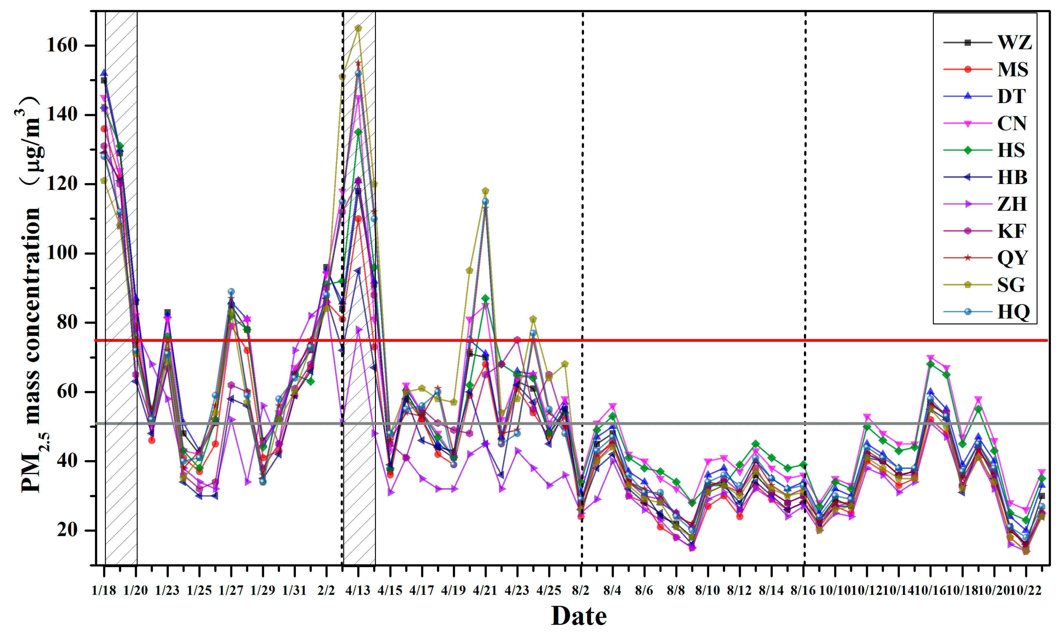
A summary of average PM2.5 mass concentrations at the11sitesduring different seasons, as well as during haze and non-haze periods (see discussion below) is shown in Table 1. The time series of PM2.5 mass concentrations at the 11 sites during the sampling periods are shown in Figure 2. The average PM2.5 mass concentration at the 11 sites during all the sampling periods was 50.7 ± 26.3 μg/m3. It was 44.9% higher than the National Ambient Air Quality Standard (NAAQS), which specifies an annual PM2.5 of 35 μg/m3 (GB3095-2012, Grade II, 2012). According to data obtained from the Environmental Protection Bureau of Wuxi, the average PM2.5 mass concentration of Wuxi was 71.2 ± 30.3 μg/m3, 61.3 ± 28.9 μg/m3, and 52.8 ± 27.5 μg/m3 in 2014, 2015, and 2016, respectively. Although the present level of PM2.5 is much higher than the NAAQS requirement, it is still about 13.9–25.8% lower than that in the past two years. This indicates that local government has taken substantial measures to reduce emissions of particles and improve the air quality, but current controls are still insufficient for the attainment of ambient air quality standards. Additionally, the accuracy of sampled PM2.5 concentrations is verified by the consistency with the Environmental Protection Bureau data. The variations in trend of PM2.5 mass concentrations observed at the 11 sites are consistent during the entire study period (Figure 2).
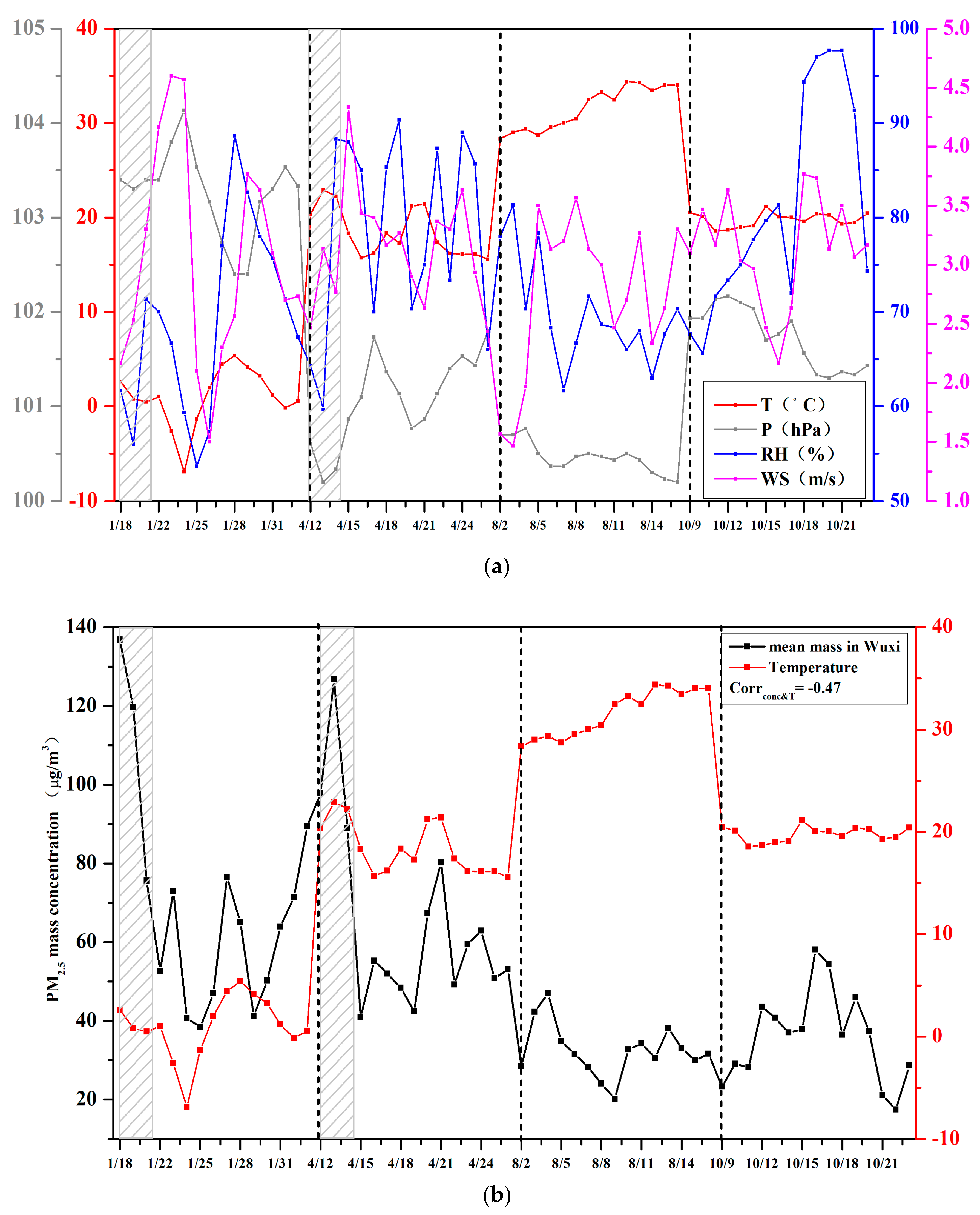
The PM2.5 mass concentrations of the four seasons decreased as follows: winter (69.4 ± 28.1 μg/m3) > spring (65.0 ± 24.1 μg/m3) > autumn (35.9 ± 11.3 μg/m3) > summer (32.4 ± 6.6 μg/m3). The daily concentrations exceeded the National 24 h Ambient Air Quality Standard (75 μg/m3) on 4 (26.7%), 4 (26.7%), 0 (0%), and 0 (0%) days for winter, spring, summer, and autumn, respectively. The air quality of summer and autumn is better than that of winter and spring. To investigate this, we compared the meteorological characteristics with the PM2.5 concentrations during the sampling periods. The meteorological data (see detail shown in Figure 3 and Table 2) were observed at11 automatic monitoring stations (nearby the sampling sites) operated by the Wuxi Environmental Monitoring Center. The correlation coefficients with PM2.5 mass concentrations were −0.47, 0.33, −0.23, and −0.16 for temperature, pressure, relative humidity, and wind speed, respectively. The correlation coefficients of temperature and pressure with PM2.5 passed the T statistical significance test within the 95% confidence interval, indicating that temperature and pressure have the closest relationship with particle concentrations. This means that conditions with high temperature and low pressure (typically in summer) are more conducive to the diffusion (especially in the vertical direction) and dilution of particulate matter. On the contrary, stable meteorological conditions in winter are more conducive to the accumulation of particles and gas-pollutant conversion into particles.
We divided the sampling sites into three functional zones: urban sites, industrial sites, and clean sites. The description of these site divisions is shown in Figure 1. During the entire period, the PM2.5 concentrations at the urban, industrial, and clean sites were 55.2 ± 26.0 μg/m3, 50.7 ± 27.3 μg/m3, and 44.2 ± 23.8 μg/m3, respectively. The average PM2.5 mass concentration of clean sites was about 15.3% lower than that of urban and industrial sites. There are no obvious industrial and coal combustion emissions within 20 km of the clean sites, so the concentrations decreased without local emissions. However, due to the meteorological conditions and the occurrence of haze episodes, the PM2.5 mass concentrations at the urban, industrial, and clean sites in winter were 74.4 ± 29.5 μg/m3, 67.8 ± 27.1 μg/m3, and 67.1 ± 29.1 μg/m3, respectively, with the industrial sites having a smaller discrepancy from the other two categories during this season. To understand this, we need to pay more attention to haze episodes. We collected samples during two sets of three-day haze episodes, which were from 18.01.2016 to 20.01.2016 and 12.04.2016 to 14.04.2016, respectively. The average PM2.5 mass concentration across all sites on haze days was 107.6 ± 25.3 μg/m3, which was 2.4 times higher than that on non-haze days (44.4 ± 17.1 μg/m3). Therefore, it is evident that fine particles significantly accumulated during the haze periods [50].
3.2. PM2.5 Chemical Compositions
The most abundant chemical components in the PM2.5 overthe entire observations were OM, SO42−, NO3−, EC, and NH4+ with mass fractions of 21.5%, 18.4%, 18.0%, 6.8%, and 6.3% of the total PM2.5 mass, respectively (shown in Figure 4). The sulfate–nitrate–ammonium ions accounted for a large fraction (42.7%) of the PM2.5 mass, and total carbon (OM and EC) contributed to 27.8% of the PM2.5 mass. Comparing these results with the mass percent of compositions of PM2.5 previously reported during haze and non-haze episodes in Beijing [40], we found that the annual mean value of the sum of the three main ions was higher in Wuxi than in Beijing (42.7% versus 35.1%), but the total carbon values in Wuxi and Beijing were almost the same (27.8% versus 27.5%). The higher sulfur content of coal in southern China, with 0.51% in the north versus 1.32% in the south of China [51], could be the reason for the higher contribution of sulfate in Wuxi (18.4%) than Beijing (14.7%). However, we found that the annual mean concentration of sulfate of PM2.5 in Wuxi was lower than in Beijing (9.31 μg/m3 versus 9.87 μg/m3). This might result from the fact that the amounts of coal consumption were larger in the Beijing-Tianjin-Hebei region than in Yangtze River Delta. The OC/EC mass ratio, which has been used to identify the presence of secondary organic aerosols, was 2.0, suggesting that there were secondary organic carbon formations [52]. However, the annual mean ratio of OC/EC in Wuxi is lower than that in Shanghai (2.6) or Beijing (3.0) [53]. The unidentified matter (UM) of the whole sampling period was about 15.6%. It is worth mentioning that one of the most abundant elements in the crust, Si, had not been analyzed in this study; this might partly account for the relatively high proportion of unidentified matter.
Crustal materials and trace elements in total account for approximately 8% of PM2.5 mass. The abundance of Ca in PM2.5 mass was 1.78 ± 1.19 μg/m3, the highest among crustal materials and trace elements. Comparing the mass concentrations of Ca among urban sites, industrial sites and clean sites, we found that it was highest in urban sites (2.02 ± 0.61 μg/m3), followed by industrial sites (1.72 ± 0.81 μg/m3), and clean sites (1.58 ± 0.51 μg/m3). Similar patterns appeared in other crustal materials. Because no obvious dust storms occurred during the entire campaign period, observations of enhanced geological material in urban sites could instead be a consequence of increasing local construction activities. The characteristics of soluble ions and carbonaceous materials in different seasons, at different site types, as well as during haze and non-haze days, are discussed in detail below (Section 3.2.1 and Section 3.2.2). Table S1 describes the concentrations of chemical components of PM2.5 during all the sampling periods.
3.2.1. Water-Soluble Ions
Water-soluble ions, such as NO2−, F−, Cl−, NO3−, SO42−, NH4+, K+, and Na+, are important chemical components in PM2.5. All of these species combined accounted for 48.3% of PM2.5 mass across the whole campaign. Inorganic secondary ions (i.e. sulfate, nitrate, and ammonium oxidized from their primary precursors) were the most abundant ions, accounting for 88.4% of all the detected ions. The mass contribution of SO42− to the PM2.5 mass showed a seasonal variation and increased in the following order: autumn (12.6%) < winter (14.5%) < spring (18.2%) < summer (33.5%). SO42− is produced from oxidation of SO2, and the availability of oxidants such as OH depends on solar radiation intensity and temperature. Therefore, in summer, sulfur dioxide is more readily converted to sulfate due to higher photochemical production of oxidants and the higher temperature-dependent reaction rates. This result of higher fractions of SO42− in summer is also consistent with the seasonal variability of SO42− previously observed in PM2.5 in Beijing [27].
The mass fractions of NO3- in observed PM2.5 mass also varied with the seasons in the following order: winter (23.2%) > spring (22.0%) > autumn (13.4%) > summer (4.0%). Because nitrate is highly volatile at high temperatures, and under cold and high humidity conditions, the formation of nitrate is much easier. Furthermore, sulfate, nitrate, and ammonium contributed much more on haze days than on non-haze days. The concentrations of sulfate, nitrate, and ammonium on haze days were about 13.6%, 33.0%, and 143.2% greater, respectively, than those on non-haze days.
The NO3−/SO42− mass ratio were used to determine the relative importance of sulfur and nitrogen in the atmosphere. The ratio of NO3−/SO42− was highest in winter (1.60) and lowest in summer (0.12) and showed the sequence from mostto leastin winter (1.60), spring (1.21), autumn (1.06), and summer (0.12), suggesting a significant contribution of sulfate in summer and nitrate in winter. Because nitrate is easily volatile at high temperature, and under cold and high humidity conditions, the formation of nitrate is easier. In the contrast, sulfate formation is favored in summer because of the higher temperature, which is more conducive to the conversion from sulfur dioxide to sulfate.
3.2.2. Organic and Elemental Carbon
Carbonaceous materials are the sum of elemental carbon and organic matter. Elemental carbon originates from primary incomplete combustion processes. Organic carbon is from both primary emission and secondary formation. Though a conversion factor from OC to OM (organic matter) can vary with many factors, such as season, emission source, and atmospheric process, in this study a factor of 1.6 is used based on previous studies [6,43].
The mass concentrations of OM of the PM2.5 decreased with the seasons in the following order: winter (17.3 ± 6.4 μg/m3) > spring (11.7 ± 4.0 μg/m3) > summer (8.4 ± 2.6 μg/m3) > autumn (6.2 ± 2.6 μg/m3). This indicates that the more stable meteorological conditions in winter are more conducive to the secondary formation of organic matter. The higher concentrations of organic aerosol in winter were also discussed in previous work, not only in China but also in some European cities [54,55]. OM accounted for 22.6%, 21.5%, and 17.7% of PM2.5 mass at industrial sites, urban sites, and clean sites, respectively. The concentrations of OM at industrial sites and urban sites were also about 46.8% and 52.1% higher than that at clean sites. This suggested that, as well as the secondary formation of organic matter, primary emissions of organic matter at industrial and urban sites also contributed significantly. We also found that OM was the most abundant component in fine particles on haze days, accounting for 35.7% of the total PM2.5 mass on these days. On non–haze days, OM only accounted for 20.2%. The total concentration of OM on haze days (38.5 ± 5.4 μg/m3) was more than four times higher than that on non-haze days (9.0 ± 5.4 μg/m3), suggesting that organic matter played a key role in PM2.5 formation on haze days. Such an observation suggested that on haze days in Wuxi, organic matter played a dominant role in haze formation.
The mass concentrations of EC in the observed PM2.5 varied with the seasons in the following order: winter (4.8 ± 2.3 μg/m3) > spring (4.0 ± 1.8 μg/m3) > autumn (2.7 ± 1.2 μg/m3) > summer (2.3 ± 1.0 μg/m3). The origination of EC reflected the primary incomplete combustion processes and was also consistent with vehicle emissions. In a similar trend to OM, EC accounted for 7.1%, 6.7%, and 5.8% of PM2.5 mass at industrial sites, urban sites, and clean sites, respectively. This indicated that, as expected, there were few primary emissions at clean sites, and the secondary formation of fine particulate matter could be the dominant contribution to PM2.5 at clean sites. EC accounted for 11.4% and 5.5% of the total PM2.5 mass on haze days and non-haze days, respectively. The concentration of EC on haze days (12.3 ± 2.1 μg/m3) was nearly five times higher than that on non-haze days (2.5 ± 1.1 μg/m3). This suggested that during the haze episode under low temperature, high pressure, breeze, and high humidity, elemental carbon could accumulate more easily.
The average OC/EC mass ratio of PM2.5 ranged from 1.44 to 2.28 over the different seasons. In winter and summer, the ratios of OC/EC were 2.25 and 2.28, respectively. However, in spring and autumn, the ratios of OC/EC were under 2. This indicated that there was significant secondary organic carbon formation in winter and lower primary emission of EC in summer. During the winter sampling period, the meteorological conditions were more conducive to the accumulation and aging of particles. Across the whole sampling period, the average ratios of OC/EC were 2.00, 2.00, and 1.90 at industrial sites, urban sites, and clean sites, respectively, suggesting the secondary generation process was largely the same at different sites. Due to the highest elemental carbon concentration on haze days, the OC/EC was slightly lower at 1.96 during haze episodes, suggesting that there may have been a slight shift towards more primary emissions on haze days. There is a large part of secondary organic aerosol in organic carbon, and it should be separated from primary emissions. In this study, the minimum value of OC/EC for each season and site type was calculated to determine the secondary organic carbon (SOC) as follows.
CSOC = CTOC − CEC × (OC/EC)min
In Equation (3), Csoc represents the concentrations of secondary organic carbon, TOC means the total organic carbon, and EC represents the elemental carbon. The concentration of SOC was converted to secondary organic matter by a factor of 1.6 [6,41]. The minimum ratio of OC to EC was 0.84, 1.33, 0.40, and 0.29 in spring, summer, autumn, and winter, respectively. Calculating with the minimum ratio of OC to EC and the conversion factor from SOC to SOA, the average concentrations of SOA were 6.44, 3.52, 4.49, and 15.09 in spring, summer, autumn, and winter, suggesting an increasing of SOA in cold weather and that OM contained larger proportion of SOA in winter.
3.3. Source Apportionment by CMB Model
Source contributions to PM2.5 were calculated using the CMB model for daily samples during the study period. A total of 15 kinds of source profiles (soil dust, cement dust, ceramic dust, straw burning, coal-fired power plant, diesel vehicle exhausts, gasoline vehicle exhausts, steel smelting, textile industry dust, cooking smoke, construction dust, secondary sulfate, secondary nitrate, sea salt, and fugitive dust) were used as model inputs for the CMB calculations. Meanwhile, a total of 27 chemical species, such as Al, As, B, Ca, Cd, Cr, Cu, Fe, Ga, Mg, Mn, Ni, P, Pb, Sr, Ti, V, NO2−, F−, Cl−, NO3−, SO42−, NH4+, K+, Na+, OC, and EC, as well as ambient PM2.5 mass, were used as input data for the CMB source apportionment analysis. The CMB model was run for all the four seasons of each site separately. Finally, we obtained 11 sets of CMB results; each set had 60 (4 seasons× 15 days/season) samples. Most of the different source emissions could be found in all the areas in Wuxi. But, some profiles were gathered in specific locations in Wuxi; for instance, the cement and ceramic industries were almost all located in the south of Wuxi, and the textile industries were mainly located in the north of Wuxi. So, in this study, profiles of cement dust and ceramic dust were only used for the measurements made at Kaifaqu (KF) and Huanbaoju (HB), and additionally, profiles of textile industry dust were only used for the measurements at Qingyang (QY), Shengang (SG), and Hongqiao (HQ).The resulting source contribution estimates (SCEs) of PM2.5 are summarized in Table 3, and the contribution fractions of different source emissions to the measured PM2.5 are also shown in Figure 5.
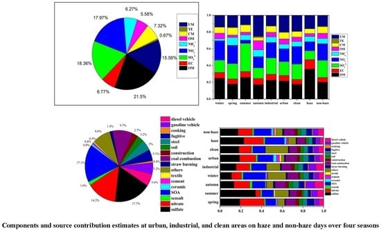
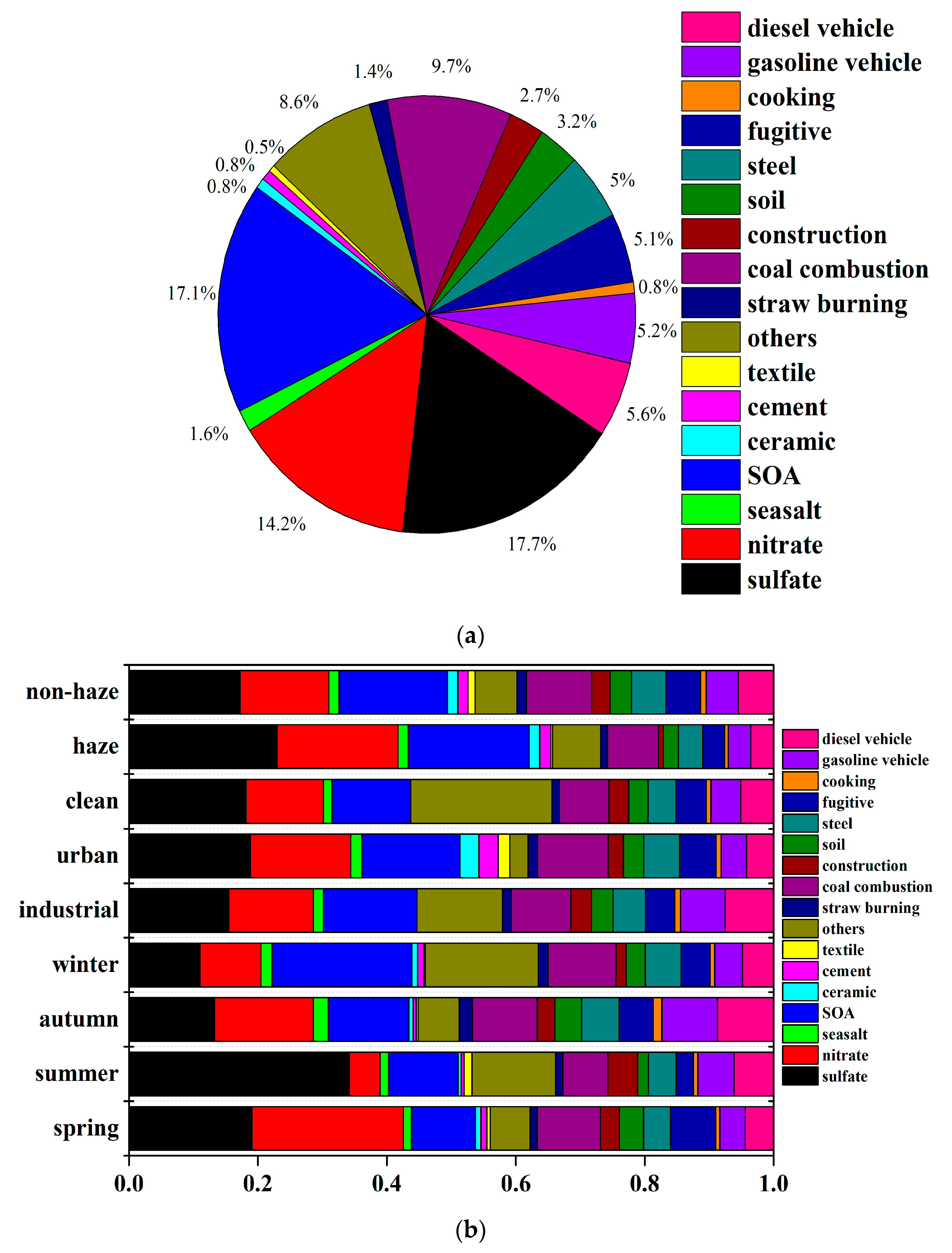
Considering the average source contributions in Wuxi during the entire sampling period (Figure 5), the contributions from primary emissions accounted for 42.4%, and those from the secondary formation processes contributed 49.0% to the total PM2.5 mass. The other 8.6% were from undefined source emissions. Secondary sulfate (17.7%), secondary organic carbon (17.1%), and secondary nitrate (14.2%) were overall the dominant sources of PM2.5 in Wuxi. The emissions from dust sources, including construction dust, soil dust, and fugitive dust, accounted for 11.1% of the total PM2.5 mass in Wuxi, indicating the influence of local construction activities to the primary fine particles. Compared with the contributions of dust previously observed in Xi’an [5] and Nanjing [21], the contribution of dust was lower in Wuxi (11.1%, measured in 2016) than that in Xi’an (19.4%, measured in 2010) and was similar to Nanjing (10.1%, measured in 2014).The sum of diesel vehicle exhausts and gasoline vehicle exhausts contributed 10.8% to PM2.5. Because vehicle exhausts could contribute to secondary aerosols, such as sulfate, nitrate, and secondary organic carbon, the contribution of vehicle exhausts could be underestimated. But, comparing with the contribution of vehicle emissions observed in Xi’an (21.3%) and in Beijing (19.6%) [39], the contribution of vehicle exhausts in Wuxi was much lower. This suggested that despite Wuxi being a major city in the Yangtze River Delta, the car density was not particularly large when compared with these other major cities in China. The next largest emission source was coal combustion, which accounted for 9.7%, indicating that coal combustion was also an important emission in Wuxi. The local industries of cement, ceramic, and textile accounted for 0.8%, 0.8%, and 0.5% of the total PM2.5, suggesting that the influences of these local industries existed but were not significant.
3.3.1. Variation in Seasons and Sites
The source contribution estimates (SCEs) for different seasons varied significantly (shown in Table 3). The contributions of dusts, including fugitive dust, construction dust, and soil dust, for the different seasons ranging from large to small were spring (8.87 μg/m3), winter (6.28 μg/m3), autumn (4.38 μg/m3), and summer (2.92 μg/m3). In spring, the dusts contributed the largest out of the four seasons, indicating more soil dust coming from bare ground in spring and the influence of dust from the north of China. In the contrast, dust contributed only 2.92 μg/m3 in summer, reflecting that Wuxi is a highly verdant city with little bare soil in summer. The SCEs of coal combustion, steel smelting and SOA had the same seasonal variation trend, showing winter > spring > autumn > summer, suggesting the meteorological conditions were conducive for the accumulation of particles both from primary emissions and organic secondary formation in winter. The SCE of secondary nitrate was highest in spring (15.27 μg/m3) and lowest in summer (1.53 μg/m3). The reasoning was similar to that of the mass fractions of NO3− of the total PM2.5 mass—that under cold and high humidity conditions, nitrogen oxide was easily converted to nitrate. The SCE of secondary sulfate showed the order of spring (12.40 μg/m3) > summer (11.10 μg/m3) > winter (7.65 μg/m3) > autumn (4.77 μg/m3). The vehicle exhausts, including both gasoline and diesel, showed a higher SCE in autumn than other seasons, suggesting that necessary control measurements should be focused on vehicle exhausts in autumn.
The source contribution estimates (SCEs) for urban, industrial and clean sites showed significant differences (shown in Table 3). The dusts, such as fugitive dust, construction dust, and soil dust, showed similar contributions at urban and industrial areas, which were 6.09 μg/m3 and 5.66 μg/m3, respectively. The SCE of dusts at clean sites (4.76 μg/m3) was slightly lower, consistent with the lack of urbanization activities around the clean sites. For other source emissions, we also found that SCEs were consistently lower at clean sites, as would be expected. The SCEs of coal combustion and steel smelting were both higher at industrial sites than those at urban sites, suggesting that primary emissions of these industries made the greatest influence on the immediate local areas. Conversely, SCEs of vehicle exhausts and cooking smoke showed higher values at urban sites than at industrial sites, due to the densities of cars, traffic jams, and restaurants in downtown areas. Secondary nitrate and secondary organic carbon both showed similar SCEs at urban and industrial sites. However, the SCEs of secondary sulfate showed somewhat higher values at industrial sites than at urban sites. This is because of the large amount of emissions of SO2 from coal combustions at industrial sites, which could convert to sulfate locally.
3.3.2. Variation between Haze and Non-Haze Days
Most SCEs of the source emissions on haze days were higher than on non-haze days, except for construction dust and textile industry emissions (shown in Table 3). The SCEs of primary sources, such as soil dust, cement dust, ceramic dust, straw burning, coal-fired power plants, diesel vehicle exhausts, gasoline vehicle exhausts, steel smelting, cooking smoke, and fugitive dust were 1.7, 2.6, 2.5, 1.7, 1.9, 1.6, 1.7, 1.7, 1.6, and 1.5 times larger than those on non-haze days. However, the SCEs of secondary sources, such as secondary sulfate, secondary nitrate, and secondary organic aerosols, were 3.2, 3.3, and 2.7 times larger than those on non-haze days. The resulting average concentration of total PM2.5 on haze days was 2.4 times larger than on non-haze days, meaning that the relative contribution fractions of primary source emissions were mostly lower on haze days than that on non-haze days. Instead, the relative contributions of secondary sulfate, secondary nitrate, and secondary organic aerosols were substantially larger on haze days than on non-haze days. This indicated that under typically cold haze days with high relative humidity, secondary particulate matter formation was the dominating reason for the much higher concentrations of particles. These parts of PM2.5 could be the secondary generations mainly from coal combustions, vehicle exhausts, and industries under the certain meteorological conditions we mentioned above. Meanwhile, the accumulation of fine particles emitted from primary sources was still an important contribution to haze formation. Thus, strict control measures, particularly on gaseous precursor emissions, as well as primary particles from coal combustion, vehicles, and industries are required on haze days.
4. Conclusions
PM2.5 concentrations and chemical compositions were sampled and analyzed during four seasons at 11 sites in 2016 in Wuxi. The annual average concentration of PM2.5 was 50.7 ± 26.3 μg/m3, which was higher than the National Ambient Air Quality Standard (Grade II) of China. Through the analysis of 17 kinds of elements and eight kinds of soluble ions and carbonaceous materials, we found that OM, SO42−, NO3−, EC, and NH4+ were the dominant chemical species in PM2.5 during this observation period, accounting for 21.5%, 18.4%, 18.0%, 6.8%, and 6.3% of the total PM2.5 mass, respectively. However, these main chemical components varied significantly in different seasons and site types. The mass fraction of SO42− washighest in summer (33.5%), and the mass fractions of NO3− were highest in winter (23.2%) and lowest in summer (4.0%). The mass concentrations of OM and EC were also highest in winter, indicating the secondary formation of organic matter. This study showed that OM and EC were the most abundant components in fine particles on haze days.
The contributions of emission sources to the ambient PM2.5 in Wuxi were calculated using the CMB model. During the entire sampling period, secondary sulfate (17.7%), secondary organic aerosols (17.1%), and secondary nitrate (14.2%) were the largest three contributions of different sources for all the 11 sites. The results showed that the dusts made the largest contribution (8.87 μg/m3) to PM2.5 in spring. The secondary organic aerosols, coal combustion, and steel smelting were higher in winter than in other seasons. The SCE of secondary nitrate was highest in spring and lowest in summer. We also found that the SCEs of secondary sources, such as secondary sulfate, secondary nitrate, and secondary organic aerosols, on haze days were much higher than on non-haze days.
For industrial sites, the SCEs of sulfate, nitrate, coal combustion, and steel smelting were highest among the three site types, indicating that primary emissions from industrial enterprises, coal-fired power plants, and secondary inorganic aerosol formation processes were the dominating sources at industrial areas. For urban sites, the SCEs of gasoline vehicle exhausts, diesel vehicle exhausts, construction dust, secondary organic aerosols, and cooking smoke showed the highest values among the three site types, indicating that the exhausts from vehicle, the dust produced by urban constructions, the secondary formation of organic aerosols, and the exhausts from cooking were the dominating sources at urban areas. For most of the source emissions, the SCEs were lower at clean sites than at industrial and urban sites. However, the CMB results of different seasons and site types, especially in winter and at clean sites also showed that considerable percentages of emissions were unidentified. More scientific work needs to be done to resolve this.
So, we should make controls for different kinds of sources at different function areas. Strict control measurements of coal combustion and industrial waste gas emissions at industrial areas are needed. Reducing urban construction activities and encouraging the use of public transportation and new energy vehicles at urban areas are also necessary changes. The results of this paper will have advisory value for local governments to create efficient policies to reduce air pollution.
Supplementary Materials
The following are available online at https://www.mdpi.com/2073-4433/9/7/267/s1, Table S1: Concentrations of chemical components in the entire sampling period (annual), four seasons, different site types, haze days, and non-haze days (μg/m3).
Author Contributions
Conceptualization, P.C. and T.W.; Methodology, P.C.; Software, P.C.; Validation, P.C. and T.W.; Formal Analysis, P.C. and T.W.; Investigation, P.C. and T.W.; Resources, T.W., and B.Z.; Data Curation, P.C., M.X.; Original Draft Preparation, P.C.; Review and Editing of the Final Manuscript, M.K., S.L., and M.L.; Visualization, P.C. and M.X.
Funding
This work was supported by the National Key Research Development Program of China (2016YFC0208504, 2017YFC0209803, 2016YFC0203303, 2014CB441203), the National Natural Science Foundation of China (91544230, 41575145, 41621005), the Prime Minister Fund (DQGG0304, DQGG0107), and the National Special Fund for the Weather Industry (GYHY201206011-1).
Acknowledgments
Thanks for the technical support from Fortelice International Co., Ltd.
Conflicts of Interest
The authors declare no conflict of interest.
References
- Dockerey, D.; Pope, A. Epidemiology of acute health effects: Summary of time-series studies. In Particles in Air: Concentration and Health Effects; Wilson, R., Spengler, J.D., Eds.; University Press: Cambridge, MA, USA, 1996. [Google Scholar]
- Seinfeld, J.H.; Pandis, S.N. Atmospheric Chemistryand Physics: From Air Pollutionto Climate Change; John Wiley & Sons, Inc.: New York, NY, USA, 2006. [Google Scholar]
- IARC (International Agency for Research on Cancer). IARC: Outdoor Air Pollution a Leading Environmental Cause of Cancer Deaths (Press Release N 221); IARC: Lyon, France, 2013. [Google Scholar]
- Remer, L.A.; Chin, M.; DeCoal, P.; Fein-gold, G.; Halthore, R.; Kahn, R.A. Aerosols and Their Climate Effects, 1–2. In Atmospheric Aerosol Properties and Climate Impacts; U.S. Climate Change Science Program Synthesis and Assessment Product 2.3; 2009. Available online: https://ntrs.nasa.gov/archive/nasa/casi.ntrs.nasa.gov/20090032661.pdf (accessed on 20 May 2018).
- Xu, H.M.; Cao, J.J.; Chow, J.C.; Huang, R.; Shen, Z.; Chen, L.; Ho, K.; Watson, J.G. Inter-annual variability of wintertime PM2.5 chemical composition in Xi’an, China: Evidences of changing source emissions. Sci. Total Environ. 2016, 545, 546–555. [Google Scholar] [CrossRef] [PubMed]
- Zhang, Y.; Cai, J.; Wang, S.; He, K.; Zheng, M. Review of receptor-based source apportionment research of fine particulate matter and its challenges in China. Sci. Total Environ. 2017, 586, 917–929. [Google Scholar] [CrossRef] [PubMed]
- Chow, J.C.; Watson, J.G. Review of PM2.5 and PM10 apportionment for fossil fuel combustion and other sources by the chemical mass balance receptor model. Energy Fuels 2002, 16, 222–260. [Google Scholar] [CrossRef]
- Antony Chen, L.; Watson, J.G.; Chow, J.C.; DuBois, D.W.; Herschberger, L. Chemical mass balance source apportionment for combined PM2.5 measurements from U.S. Non-urban and Urban Long-term networks. Atmos. Environ. 2010, 44, 4908–4918. [Google Scholar] [CrossRef]
- Deshmukh, D.K.; Deb, M.K.; Tsai, Y.I.; Mkoma, S.L. Water soluble ions in PM2.5 and PM2.1 aerosols in Durg City, Chhattisgarh, India. Aerosol Air Qual. Res. 2011, 11, 696–708. [Google Scholar]
- Chan, C.K.; Yao, X. Air pollution in mega cities in China. Atmos. Environ. 2008, 42, 1–42. [Google Scholar] [CrossRef]
- Belis, C.A.; Karagulian, F.; Amato, F.; Almeida, M.; Artaxo, P.; Beddows, D.C.S.; Bernardoni, V.; Bove, M.C.; Carbone, S.; Cesari, D. A new methodology to assess the performance and uncertainty of source apportionment models II: The results of teo European intercomparison exercises. Atmos. Environ. 2015, 123, 240–250. [Google Scholar] [CrossRef] [Green Version]
- Cesari, D.; Donateo, A.; Conte, M.; Contini, D. Inter-comparison of source apportionment of PM10 using PMF and CMB in three sites nearby an industrial area in central Italy. Atmos. Res. 2016, 182, 282–293. [Google Scholar] [CrossRef]
- Wang, H.L.; Zhuang, Y.H.; Wang, Y.; Sun, Y.L.; Yuan, H.; Zhuang, G.S.; Hao, Z. Long-term monitoring and source apportionment of PM2.5/PM10 in Beijing, China. J. Environ. Sci. 2008, 20, 1323–1327. [Google Scholar] [CrossRef]
- Xie, S.D.; Liu, Z.; Chen, T.; Hua, L. Spatiotemporal variations of ambient PM10 source contributions in Beijing in 2004 using positive matrix factorization. Atmos. Chem. Phys. 2008, 8, 2701–2716. [Google Scholar] [CrossRef]
- Deng, J.J.; Wang, T.J.; Jiang, Z.Q.; Xie, M.; Zhang, R.J.; Huang, X.X.; Zhu, J.L. Characterization of visibility and its affecting factors over Nanjing, China. Atmos. Res. 2011, 101, 681–691. [Google Scholar] [CrossRef]
- Xu, H.M.; Cao, J.J.; Ho, K.F.; Ding, H.; Han, Y.M.; Wang, G.H.; Chow, J.C.; Watson, J.G.; Khol, S.D.; Qiang, J.; et al. Lead concentrations in fine particulate matter after the phasing out of leaded gasoline in Xi’an, China. Atmos. Environ. 2012, 46, 217–224. [Google Scholar] [CrossRef]
- Zhu, C.S.; Cao, J.J.; Shen, Z.X.; Liu, S.X.; Zhang, T.; Zhao, Z.Z.; Xu, H.; Zhang, E. Indoor and outdoor chemical components of PM2.5 in the rural areas of Northwestern China. Aerosol Air Qual. Res. 2012, 12, 1157–1165. [Google Scholar] [CrossRef]
- Wang, P.; Cao, J.J.; Shen, Z.X.; Han, Y.M.; Lee, S.C.; Huang, Y.; Zhu, C.S.; Wang, Q.Y.; Xu, H.M.; Huang, R.J. Spatial and seasonal variations of PM2.5 mass and species during 2010 in Xi’an, China. Sci. Total Environ. 2015, 508, 477–487. [Google Scholar] [CrossRef] [PubMed]
- Chen, P.L.; Wang, T.J.; Hu, X. Chemical Mass Balance Source Apportionment of Size-Fractionated Particulate Matter in Nanjing, China. Aerosol Air Qual. Res. 2015, 15, 1855–1867. [Google Scholar] [CrossRef]
- Deng, J.J.; Zhang, Y.R.; Hong, Y.W.; Xu, L.L.; Chen, Y.T.; Du, W.J.; Chen, J.S. Optical properties of PM2.5 and the impacts of chemical compositions in the coastal city Xiamen in China. Sci. Total Environ. 2016, 557, 665–675. [Google Scholar] [CrossRef] [PubMed]
- Chen, P.; Wang, T.; Lu, X.; Yu, Y.; Kasoar, M.; Xie, M.; Zhuang, B. Source apportionment of size-fractionated particles during the 2013 Asian Youth Games and the 2014 Youth Olympic Games in Nanjing, China. Sci. Total Environ. 2017, 579, 860–870. [Google Scholar] [CrossRef] [PubMed]
- He, K.B.; Huo, H.; Zhang, Q. Urban air pollution in China: Current status, characterizes and progress. Annu. Rev. Energy Environ. 2002, 27, 397–431. [Google Scholar] [CrossRef]
- Tie, X.; Cao, J. Aerosol pollution in China: Present and future impact on environment. Particuology 2009, 7, 426–431. [Google Scholar] [CrossRef]
- Gao, M.; Guttikunda, S.K.; Carmichael, G.R.; Wang, Y.; Liu, Z.; Stanier, C.O. Health impacts and economic losses assessment of the 2013 severe haze event in Beijing area. Sci. Total Environ. 2015, 511, 553–561. [Google Scholar] [CrossRef] [PubMed]
- Han, B.; Bi, X.H.; Xue, Y.; Wu, J.; Zhu, T.; Zhang, B.; Ding, J.; Du, Y. Source apportionment of ambient PM10 in urban areas of Wuxi, China. Front. Environ. Sci. Eng. 2011, 5, 552–563. [Google Scholar] [CrossRef]
- Wang, T.J.; Jiang, F.; Deng, J.J.; Shen, Y.; Fu, Q.Y.; Wang, Q.; Fu, Y.; Xu, J.H.; Zhang, D.N. Urban air quality and regional haze weather forecast for Yangtze River Delta region. Atmos. Environ. 2012, 58, 70–83. [Google Scholar] [CrossRef]
- Zhang, R.; Jing, J.; Tao, J.; Hsu, S.C.; Wang, G.; Cao, J.; Lee, C.; Zhu, L.; Chen, Z.; Zhao, Y.; et al. Chemical characterization and source apportionment of PM2.5 in Beijing: Seasonal perspective. Atmos. Chem. Phys. 2013, 13, 7053–7074. [Google Scholar] [CrossRef]
- Zhang, Y.F.; Xu, H.; Tian, Y.Z.; Shia, G.L.; Zeng, F.; Wu, J.H.; Zhang, X.Y.; Li, X.; Zhu, T.; Feng, Y.C. The Study on Vertical Variability of PM10 and the Possible Sources on a 220 m Tower in Tianjin China. Atmos. Environ. 2011, 45, 6133–6140. [Google Scholar] [CrossRef]
- Fu, Q.; Zhuang, G.; Wang, J.; Xu, C.; Huang, K.; Li, J.; Hou, B.; Lu, T.; Streets, D.G. Mechanism of formation of the heaviest pollution episode ever recorded in the Yangtze River Delta, China. Atmos. Environ. 2008, 42, 2023–2036. [Google Scholar] [CrossRef]
- Wang, Y.; Zhuang, G.; Zhang, X.; Zhang, X.; Huang, K.; Xu, C.; Tang, A.; Chen, J.; An, Z. The ion chemistry, seasonal cycle, and sources of PM2.5 and TSP aerosol in Shanghai. Atmos. Environ. 2006, 40, 2935–2952. [Google Scholar] [CrossRef]
- Ambient Air Quality Standards in China; GB3095-2012; Ministry of Environmental Protection and General Administration of Quality Supervision, Inspection and Quarantine of the People’s Republic of China: Beijing, China, 2012.
- Tan, J.H.; Duan, J.C.; Chen, D.H.; Wang, X.H.; Guo, S.J.; Bi, X.H.; Sheng, G.Y.; He, K.B.; Fu, J.M. Chemical characteristics of haze during summer and winter in Guangzhou. Atmos. Res. 2009, 94, 238–245. [Google Scholar] [CrossRef]
- Sun, Y.; Zhuang, G.; Tang, A.; Wang, Y.; An, Z. Chemical characteristics of PM2.5 and PM10 in haze-fog episodes in Beijing. Environ. Sci. Technol. 2006, 40, 3148–3155. [Google Scholar] [CrossRef] [PubMed]
- Zhuang, X.; Wang, Y.; He, H.; Liu, J.; Wang, X.; Zhu, T.; Ge, M.; Zhou, J.; Tang, G.; Ma, J. Haze insights and mitigation in China: An overview. J. Environ. Sci. 2014, 26, 2–12. [Google Scholar] [CrossRef] [Green Version]
- Chen, P.; Wang, T.; Dong, M.; Kasoar, M.; Han, Y.; Xie, M.; Li, S.; Zhuang, B.; Li, M.; Huang, T. Characterization of major natural and anthropogenic source profiles for size-fractionated PM in Yangtze River Delta. Sci. Total Environ. 2017, 598, 135–145. [Google Scholar] [CrossRef] [PubMed]
- Chow, J.C.; Watson, J.G.; Pritchett, L.C.; Pierson, W.R.; Frazier, C.A.; Purcell, R.G. The dri thermal/optical reflectance carbon analysis system: Description, evaluation and applications in U.S. air quality studies. Atmos. Environ. 1993, 27, 1185–1201. [Google Scholar] [CrossRef]
- Chow, J.C.; Watson, J.G.; Chen, L.W.A.; Arnott, W.P.; Moosmuller, H. Equivalence of elemental carbon by thermal/optical reflectance and transmittance with different temperature protocols. Environ. Sci. Technol. 2004, 38, 4414–4422. [Google Scholar] [CrossRef] [PubMed]
- Chow, J.C.; Watson, J.G.; Chen, L.W.A.; Paredes-Mir, G.; Chang, M.C.O.; Trimble, D. Atmospheric chemistry and physics refining temperature measures in thermal/optical carbon analysis. Atmos. Chem. Phys. 2005, 5, 2961–2972. [Google Scholar] [CrossRef]
- Tian, S.L.; Pan, Y.P.; Wang, Y.S. Size-resolved source apportionment of particulate matter in urban Beijing during haze and non-haze episodes. Atmos. Chem. Phys. 2016, 16, 1–19. [Google Scholar] [CrossRef]
- Tan, J.; Duan, J.; Zhen, N.; He, K.; Hao, J. Chemical characteristics and source of size-fractionated atmospheric particle in haze episode in Beijing. Atmos. Res. 2016, 167, 24–33. [Google Scholar] [CrossRef]
- Kunwar, B.; Kawamura, K. One-year observations of carbonaceous and nitrogenous components and major ions in the aerosols from subtropical Okinawa Island, an outflow region of Asian dusts. Atmos. Chem. Phys. 2014, 14, 1819–1836. [Google Scholar] [CrossRef] [Green Version]
- Yao, L.; Yang, L.X.; Yuan, Q.; Yan, C.; Dong, C.; Meng, C. Source apportionment of PM2.5 in a background site in the North China Plain. Sci. Total Environ. 2016, 541, 590–598. [Google Scholar] [CrossRef] [PubMed]
- Chan, T.W.; Huang, L.; Leaitch, W.R.; Sharma, S.; Brook, J.R.; Slowik, J.G. Observations of OM/OC and specific attenuation coefficients (SAC) in ambient fine PM at a rural site ini central Ontario, Canada. Atmos. Chem. Phys. 2010, 10, 2393–2411. [Google Scholar] [CrossRef]
- Thurston, G.D.; Spengler, J.D. A quantitative assessment of source contributions to inhalable particulate matter pollution in metropolitan Boston. Atmos. Environ. 1985, 19, 9–25. [Google Scholar] [CrossRef]
- Watson, J.G.; Cooper, J.A.; Huntzicker, J.J. The effective variance weighting for least squares calculations applied to the mass balance receptor model. Atmos. Environ. 1984, 18, 1347–1355. [Google Scholar] [CrossRef]
- Paatero, P.; Tapper, U. Positive matrix factorization: A non-negative factor model with optimal utilization of error estimates of data values. Environmetrics 1994, 5, 111–126. [Google Scholar] [CrossRef]
- Kong, S.; Han, B.; Bai, Z.; Chen, L.; Shi, J.; Xu, Z. Receptor Modeling of PM2.5, PM10 and TSP in Different Seasons and Long-range Transport Analysis at A coastal Site of Tianjin, China. Sci. Total Environ. 2010, 408, 4681–4694. [Google Scholar] [CrossRef] [PubMed]
- Wu, H.; Zhang, Y.; Han, S.; Wu, J.; Bi, X.; Shi, G.; Wang, J.; Yao, Q.; Cai, Z.; Liu, J.; et al. Vertical characteristics of PM2.5 during the heating season in Tianjin, China. Sci. Total Environ. 2015, 523, 152–160. [Google Scholar] [CrossRef] [PubMed]
- US EPA. EPA-CMB8.2 User’s Manual; EPA-452/R-04-011; US EPA: Research Triangle Park, NC, USA, 2004.
- Wang, L.T.; Wei, Z.; Yang, J.; Zhang, Y.; Zhang, F.; Su, J.; Meng, C.C.; Zhang, Q. The 2013 severe haze over southern Hebei, China: Model evaluation, source apportionment, and policy implications. Atmos. Chem. Phys. 2014, 14, 3151–3173. [Google Scholar] [CrossRef] [Green Version]
- Lu, Z.; Streets, D.G.; Zhang, Q.; Wang, S.; Carmichael, G.R.; Cheng, Y.F. Sulfur dioxide emissions in China and sulfur trends in East Asia since 2000. Atmos. Chem. Phys. 2010, 10, 6311–6331. [Google Scholar] [CrossRef] [Green Version]
- Turpin, B.J.; Cary, R.A.; Huntzicker, J.J. An in-situ, time-resolved analyzer for aerosol organic and elemental carbon. Aerosol Sci. Technol. 1990, 12, 161–171. [Google Scholar] [CrossRef]
- Yang, F.; Tan, J.; Zhao, Q.; Du, Z.; He, K.; Ma, W.; Duan, F.; Chen, G.; Zhao, Q. Characteristics of PM2.5 speciation in representative megacities and across China. Atmos. Chem. Phys. 2011, 11, 5207–5219. [Google Scholar] [CrossRef]
- Cesari, D.; Merico, E.; Dinoi, A.; Marinoni, A.; Bonasoni, P.; Contini, D. Seasonal variability of carbonaceous aerosols in an urban background area in Southern Italy. Atmos. Res. 2018, 200, 97–108. [Google Scholar] [CrossRef]
- Khan, M.B.; Masiol, M.; Formenton, G.; Di Gilio, A.; de Gennaro, G.; Agostinelli, C.; Pavoni, B. Carbonaceous PM2.5 and secondary organic aerosol across the Veneto region (NE Italy). Sci. Total Environ. 2016, 542, 172–181. [Google Scholar] [CrossRef] [PubMed]
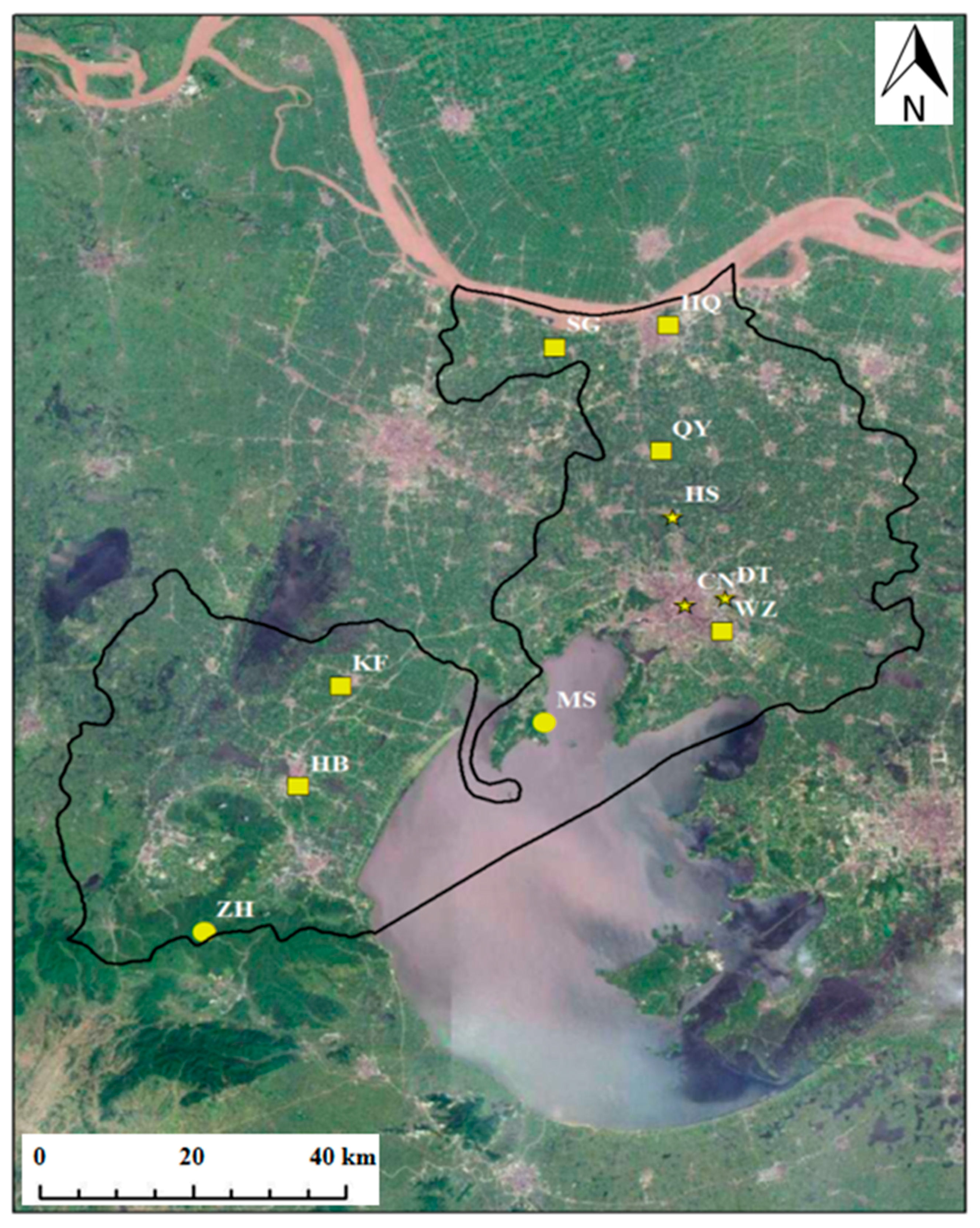
Figure 1.
Sampling sites. In these 11 sites, urban sites (Dongting (DT), Chongning (CN), Huishan (HS)) are represented in yellow pentacles, industrial sites (Huanbaoju (HB), Kaifaqu (KF), Qingyang (QY), Shengang (SG), Hongqiao (HQ), Wangzhuang (WZ)) are represented in yellow squares, and clean sites (Mashan (MS), Zhuhai (ZH)) are represented in yellow circles. The black solid line marks the scope of Wuxi.

Figure 2.
Fine particulate matter (PM2.5) mass concentrations of 11 sites (grey solid line represents average concentration (50.7 μg/m3) of all the 11sites in 2016, red solid line represents National Standard of PM2.5, black dashed lines divide four sampling periods, and the shades areas represent the haze periods).

Figure 3.
Temperature, pressure, relative humidity, and wind speed measurements during the sampling periods (a). PM2.5 mass concentrations and temperature measurements during the sampling periods (b).
Figure 3.
Temperature, pressure, relative humidity, and wind speed measurements during the sampling periods (a). PM2.5 mass concentrations and temperature measurements during the sampling periods (b).

Figure 4.
Chemical species contributed to the total PM2.5 mass concentrations during the entire sampling period (a). Chemical species contributed to the total PM2.5 mass concentrations at different seasons and different sites, as well as haze or non-haze days (b). Abbreviations: organic matter (OM), crustal materials (CM), sulfate (SO42−), nitrate (NO3−), ammonium (NH4+), elemental carbon (EC), soluble ions except sulfate, nitrate and ammonium (O(ther)SI), trace elements (TE), and unidentified matter (UM).
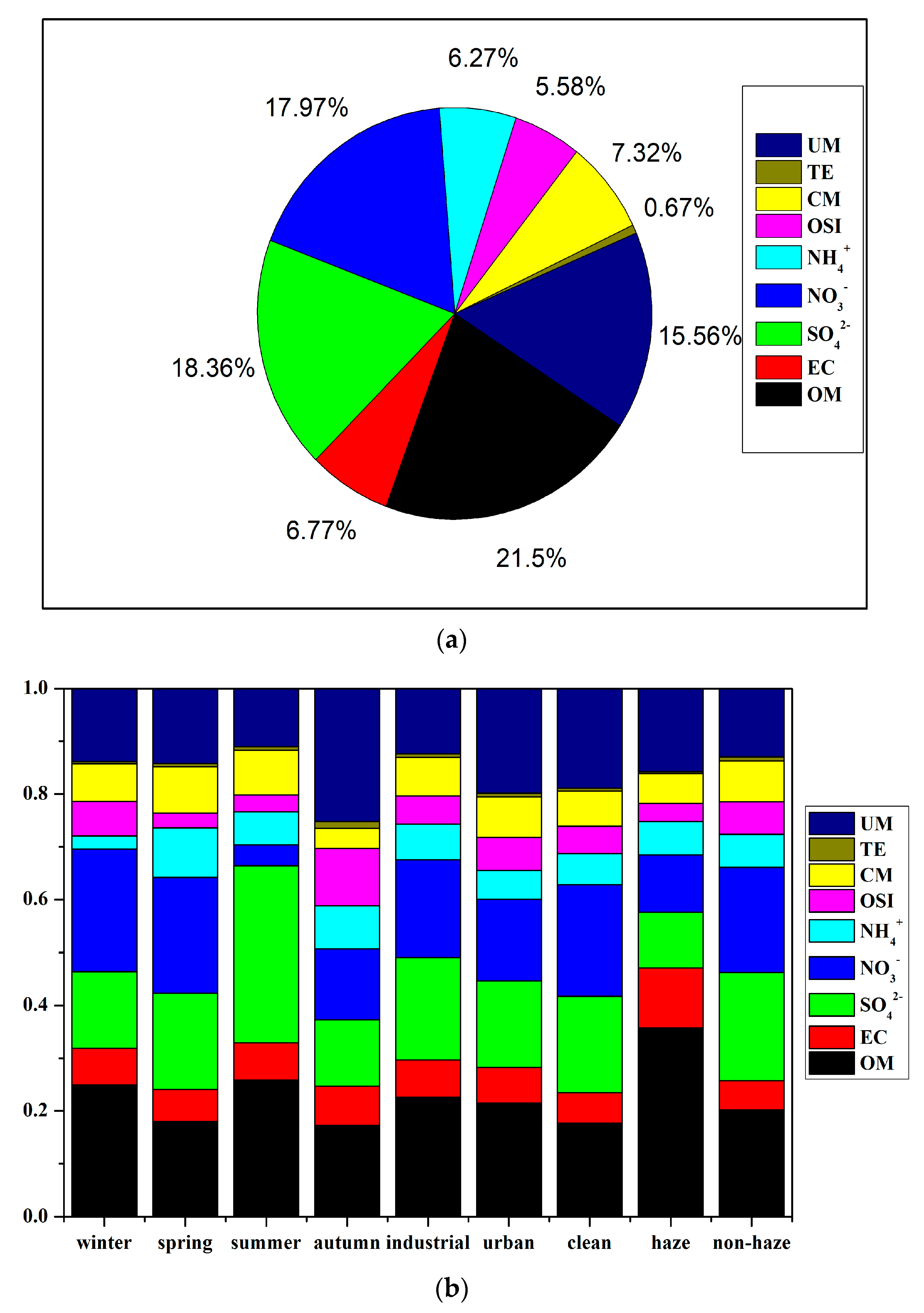
Figure 5.
Source contribution fractions to the total PM2.5 mass during the entire sampling period (a). Chemical species contributed to the total PM2.5 mass concentrations at different seasons and different sites, as well as haze or non-haze days (b).
Figure 5.
Source contribution fractions to the total PM2.5 mass during the entire sampling period (a). Chemical species contributed to the total PM2.5 mass concentrations at different seasons and different sites, as well as haze or non-haze days (b).


Table 1.
Summary of average PM2.5 mass concentrations (μg/m3) of 11sites of different seasons as well as during hazeand non-haze periods.
Table 1.
Summary of average PM2.5 mass concentrations (μg/m3) of 11sites of different seasons as well as during hazeand non-haze periods.
| Site | DT | CN | HS | HB | KF | QY | SG | HQ | WZ | MS | ZH |
|---|---|---|---|---|---|---|---|---|---|---|---|
| Type | Urban | Industrial | Clean | ||||||||
| Mean a | 53.4 ± 26.5 b | 56.9 ± 26.3 | 55.2 ± 25.3 | 44.9 ± 22.3 | 49.0 ± 25.2 | 52.6 ± 28.7 | 53.4 ± 32.0 | 53.1 ± 28.3 | 51.2 ± 27.0 | 47.2 ± 25.0 | 41.2 ± 22.7 |
| Winter | 76.7 ± 30.3 | 74.1 ± 28.8 | 72.3 ± 29.5 | 61.7 ± 29.3 | 64.0 ± 28.6 | 69.6 ± 25.1 | 66.3 ± 24.1 | 69.3 ± 25.3 | 75.7 ± 30.2 | 68.5 ± 28.6 | 65.7 ± 29.6 |
| Spring | 64.6 ± 21.4 | 69.9 ± 27.9 | 67.3 ± 24.8 | 54.9 ± 14.8 | 65.9 ± 23.3 | 73.3 ± 33.0 | 83.9 ± 36.2 | 73.2 ± 32.7 | 62.7 ± 21.0 | 58.5 ± 18.3 | 41.1 ± 11.6 |
| Summer | 34.6 ± 7.3 | 39.3 ± 6.8 | 38.8 ± 6.3 | 29.2 ± 6.2 | 31.8 ± 5.8 | 32.7 ± 5.9 | 30.9 ± 6.3 | 33.7 ± 6.6 | 31.1 ± 7.7 | 28.0 ± 7.7 | 26.9 ± 5.7 |
| Autumn | 37.9 ± 10.8 | 44.4 ± 13.2 | 42.3 ± 13.1 | 33.9 ± 11.0 | 34.4 ± 11.3 | 34.8 ± 11.2 | 32.7 ± 11.1 | 36.1 ± 11.0 | 35.2 ± 11.1 | 32.7 ± 10.6 | 31.1 ± 10.3 |
| Haze | 111.3 ± 24.8 | 115.8 ± 26.3 | 111.8 ± 25.2 | 91.2 ± 26.1 | 106.2 ± 22.7 | 116.0 ± 24.1 | 122.7 ± 30.2 | 114.8 ± 23.9 | 109.7 ± 24.6 | 100.2 ± 23.8 | 84.2 ± 26.1 |
| Non-haze | 47.0 ± 17.2 | 50.4 ± 16.2 | 48.9 ± 15.7 | 39.8 ± 14.5 | 42.7 ± 15.6 | 45.5 ± 18.9 | 45.7 ± 21.0 | 46.2 ± 18.9 | 44.7 ± 18.0 | 41.2 ± 16.7 | 36.4 ± 15.0 |
a the average PM2.5 concentrations of the whole sampling period in 2016. b standard deviation.
Table 2.
Meteorological characteristics during the sampling periods and the correlation coefficient with PM2.5 mass.
Table 2.
Meteorological characteristics during the sampling periods and the correlation coefficient with PM2.5 mass.
| Meteorological Parameters | Correlation with PM2.5 Mass | |
|---|---|---|
| Temperature (°C) | 17.7 ± 11.2 a | −0.47 |
| Pressure (hPa) | 101.6 ± 1.1 | 0.33 |
| Relative humidity (%) | 74.7 ± 10.7 | −0.23 |
| Wind speed (m/s) | 3.0 ± 0.7 | −0.16 |
a standard deviation.
Table 3.
Average source contribution estimates (SCEs) of PM2.5 mass concentrations using chemical mass balance (CMB) models (μg/m3).
Table 3.
Average source contribution estimates (SCEs) of PM2.5 mass concentrations using chemical mass balance (CMB) models (μg/m3).
| Winter | Spring | Summer | Autumn | Industrial | Urban | Clean | Haze | Non-Haze | |
|---|---|---|---|---|---|---|---|---|---|
| straw burning | 1.03 | 0.73 | 0.37 | 0.71 | 0.76 | 0.75 | 0.51 | 1.11 | 0.64 |
| coal combustion | 7.34 | 6.38 | 2.25 | 3.63 | 5.53 | 5.09 | 3.37 | 8.56 | 4.48 |
| construction | 1.09 | 1.92 | 1.51 | 0.99 | 1.20 | 1.76 | 1.35 | 0.79 | 1.31 |
| soil | 2.05 | 2.40 | 0.54 | 1.49 | 1.60 | 1.85 | 1.32 | 2.47 | 1.46 |
| steel | 3.87 | 2.74 | 1.40 | 2.09 | 2.82 | 2.80 | 1.90 | 4.13 | 2.38 |
| fugitive | 3.14 | 4.55 | 0.87 | 1.90 | 2.85 | 2.49 | 2.09 | 3.62 | 2.38 |
| cooking | 0.52 | 0.43 | 0.22 | 0.48 | 0.41 | 0.49 | 0.30 | 0.60 | 0.37 |
| gasoline vehicle | 2.99 | 2.57 | 1.83 | 3.09 | 1.98 | 3.81 | 2.04 | 3.77 | 2.23 |
| diesel vehicle | 3.35 | 2.86 | 1.98 | 3.13 | 2.13 | 4.16 | 2.25 | 3.81 | 2.43 |
| sulfate | 7.65 | 12.40 | 11.10 | 4.77 | 9.54 | 8.53 | 8.00 | 24.70 | 7.65 |
| nitrate | 6.60 | 15.27 | 1.53 | 5.50 | 7.87 | 7.27 | 5.27 | 20.19 | 6.10 |
| Sea salt | 1.18 | 0.83 | 0.43 | 0.81 | 0.87 | 0.85 | 0.58 | 1.66 | 0.71 |
| SOA | 15.09 | 6.44 | 3.52 | 4.49 | 7.69 | 7.99 | 5.38 | 20.22 | 7.76 |
| ceramic | 0.63 | 0.55 | 0.14 | 0.23 | 1.49 | -- | -- | 1.76 | 0.71 |
| cement | 0.67 | 0.59 | 0.15 | 0.18 | 1.52 | -- | -- | 1.88 | 0.72 |
| textile | 0.14 | 0.35 | 0.40 | 0.10 | 0.93 | -- | -- | 0.31 | 0.48 |
| others | 12.25 | 4.02 | 4.21 | 2.30 | 1.43 | 7.36 | 9.66 | 8.02 | 4.15 |
© 2018 by the authors. Licensee MDPI, Basel, Switzerland. This article is an open access article distributed under the terms and conditions of the Creative Commons Attribution (CC BY) license (http://creativecommons.org/licenses/by/4.0/).
Share and Cite
MDPI and ACS Style
Chen, P.; Wang, T.; Kasoar, M.; Xie, M.; Li, S.; Zhuang, B.; Li, M. Source Apportionment of PM2.5 during Haze and Non-Haze Episodes in Wuxi, China. Atmosphere 2018, 9, 267. https://doi.org/10.3390/atmos9070267
AMA Style
Chen P, Wang T, Kasoar M, Xie M, Li S, Zhuang B, Li M. Source Apportionment of PM2.5 during Haze and Non-Haze Episodes in Wuxi, China. Atmosphere. 2018; 9(7):267. https://doi.org/10.3390/atmos9070267
Chicago/Turabian StyleChen, Pulong, Tijian Wang, Matthew Kasoar, Min Xie, Shu Li, Bingliang Zhuang, and Mengmeng Li. 2018. "Source Apportionment of PM2.5 during Haze and Non-Haze Episodes in Wuxi, China" Atmosphere 9, no. 7: 267. https://doi.org/10.3390/atmos9070267
Note that from the first issue of 2016, this journal uses article numbers instead of page numbers. See further details here.