Current Challenges in Understanding and Predicting Transport and Exchange in the Atmosphere over Mountainous Terrain


Department of Atmospheric and Cryospheric Sciences, University of Innsbruck; 6020 Innsbruck, Austria
*
Author to whom correspondence should be addressed.
Atmosphere 2018, 9(7), 276; https://doi.org/10.3390/atmos9070276
Submission received: 8 June 2018
/
Revised: 9 July 2018
/
Accepted: 14 July 2018
/
Published: 18 July 2018
(This article belongs to the Special Issue Atmospheric Processes over Complex Terrain)
Abstract
:Coupling of the earth’s surface with the atmosphere is achieved through an exchange of momentum, energy, and mass in the atmospheric boundary layer. In mountainous terrain, this exchange results from a combination of multiple transport processes, which act and interact on different spatial and temporal scales, including, for example, orographic gravity waves, thermally driven circulations, moist convection, and turbulent motions. Incorporating these exchange processes and previous studies, a new definition of the atmospheric boundary layer in mountainous terrain, a mountain boundary layer (MBL), is defined. This paper summarizes some of the major current challenges in measuring, understanding, and eventually parameterizing the relevant transport processes and the overall exchange between the MBL and the free atmosphere. Further details on many aspects of the exchange in the MBL are discussed in several other papers in this issue.
1. Introduction
Mountainous areas contribute in major ways to atmospheric flows at a wide range of spatial scales. Clearly, a mountain range such as the Alps, the Rocky Mountains or the Himalayas constitutes an obstacle to the hemispheric or synoptic-scale flow and has sufficient vertical extension to substantially modify the geopotential fields in its vicinity so as to trigger thermodynamic responses (e.g., orographic precipitation [1]), periodic perturbations (e.g., gravity waves [2,3]) or instabilities (e.g., lee cyclogenesis [4,5]). The impact of mountains on the atmosphere is communicated through the atmospheric boundary layer (ABL), where different processes can effectuate an exchange of momentum, energy, moisture, and other atmospheric components between the earth’s surface and the atmosphere. While these processes are mainly restricted to vertical turbulent mixing over flat terrain, a multitude of additional processes can contribute to the exchange at different spatial and temporal scales in mountainous terrain [6]. The role of the atmospheric boundary layer in the climate system, that is, to effectuate the earth-atmosphere interaction, is thus extended in scale (to mesoscale flows at least), complexity (to non-homogeneous conditions at least), and possibly also effectiveness. This review attempts to give a comprehensive overview of the processes contributing to this exchange over complex terrain and in particular, to highlight current deficiencies in our understanding of the ABL over mountainous terrain and subsequently, in our treatment of the ABL in numerical weather prediction (NWP) models. The problem begins with the definition of the ABL over mountainous terrain. As will be shown in Section 3, the ABL over mountainous terrain exhibits oftentimes a more complex, multi-layered structure (e.g., [7]) so that existing methods to determine the ABL height over flat terrain can be inefficient in describing the boundary-layer height. For this reason, a new mountain boundary layer (MBL) will be defined.
In the 70s/80s of the past century, research efforts to better understand the large-scale processes were coordinated in the Alpine Experiment (ALPEX [8,9]) and later in the Momentum Budget over the Pyrénées Experiment (PYREX [10]). Mesoscale aspects and refinements of the above synoptic-scale processes were investigated in another large international effort, that is, the Mesoscale Alpine Programme (MAP [11,12]), which culminated in a coordinated field phase in 1999 [13]. MAP was the first Research and Development Project of the World Weather Research Programme of the World Meteorological Organization (WMO) and, as such, also addressed an application aspect, in this case mountain hydrology [14]. Operational high-resolution NWP for Alpine hydrological forecasts was consequently the topic of a World Weather Research Programme Forecast Demonstration Project (MAP D-PHASE) that aimed at demonstrating the advances in operational procedures due to coordinated research [15,16].
With the advance of computing power (and hence the possibility to perform high-resolution numerical simulations) and the availability of advanced observational technology, it is not only possible to study the various processes of the near-surface atmosphere over complex mountainous terrain in isolation and under idealized conditions (e.g., the turbulence structure over an infinite slope, the thermally driven valley and slope flows in a straight valley, the excitation of gravity waves over a sine-shaped ridge, etc.), but also to address the problem of how these processes interact and how these interactions impact their effectivity to transport mass, momentum, and energy from and to the earth’s surface. While these processes are mainly restricted to vertical turbulent mixing over flat terrain, complex interactions and feedback can still occur (see, e.g., an overview in Santanello et al. [17]), stimulating recent and current efforts to further our understanding of land-atmosphere interactions, including the ScaleX experiment [18] and the Global Energy and Water Exchanges project (GEWEX) Global Land-Atmosphere System Study (GLASS; [19]) focus on Land-Atmosphere coupling (LoCo; [17]).
On a large scale, local climate change in mountain areas may differ from global average trends and may lead to topography-specific regional effects (see, for example, the review of climate change in the Alpine region by Gobiet et al. [20]). For example, the temperature increase in the Greater Alpine region has been twice as high as the average over the entire northern hemisphere between the late 19th century and the end of the 20th century [21] and changes in precipitation over the past decades are not consistent across the entire Alpine region, but rather values and signs differ between regions and seasons [20,22]. An important aspect in mountainous terrain is the altitudinal range of the surface. An elevation dependency has been found for the past humidity trend in the Alpine region [22], as well as for future temperature and precipitation trends [23]. Temperature changes in a changing climate are influenced by, for example, snow-albedo feedback processes and thus changes in the snowpack [24]. The resulting temperature changes with height can thus depend on the region, with either an increase in the warming with height or a decrease [25]. The effects of a changing climate in complex terrain will also have the potential to impact future frequencies of heavy precipitation events [26], droughts [27], forest damage from storms [28], and water supplies as mountain runoff is a major water source [29].
Figure 1 depicts examples from the literature, in which the transport of momentum, heat, and moisture (i.e., mass) over mountainous terrain has been investigated based on observations, idealized numerical modeling, or real-terrain numerical simulations. The corresponding processes and challenges are discussed in more detail below (Section 3.2 and Section 4). Here, we want to emphasize that (missing) momentum transport due to orographic gravity wave drag and sub-grid scale topography has long been identified as a source of systematic bias in global circulation and numerical weather prediction models [30]. It is thus parameterized nowadays in one way or the other in global and mesoscale NWP or climate models. For energy exchange (sensible heat), the importance of terrain flows was first suggested by Noppel and Fiedler [31] and a number of idealized-terrain studies have attempted to systematically assess relevant parameters and the magnitude of this exchange (Section 3.2.3). A parameterization for large-scale numerical models, however, is still missing. For mass, such as moisture or air pollutants, to the knowledge of the authors, only case studies from individual or idealized valleys are available (e.g., the one in Figure 1) that highlight the potential of mass exchange for certain geographic areas or seasons (e.g., [32]). Only when numerical models develop from atmospheric weather and climate models into environmental prediction systems, will the question of a sub-grid scale parameterization of mass exchange likely become relevant.
In the remainder of this paper we will use the following definitions for the terms transport and exchange. Transport is the general conveyance of a quantity, for example, heat, mass, or momentum, either within a defined volume or between different defined volumes, such as the valley atmosphere or the MBL. The term mass always includes moisture and other atmospheric components, such as, for example, aerosols or CO2. Exchange, on the other hand, refers specifically to the conveyance or transport of a quantity into a different volume or through an interface, for example, a transport of mass from the MBL into the free atmosphere aloft or from the surface to the atmosphere. An exchange process can also be considered a simultaneous transport in both directions, where, for example, a positive energy transport from the MBL to the atmosphere aloft is equivalent to a negative energy transport from the atmosphere aloft to the MBL, thus constituting an exchange of energy between the two volumes.
2. Current Research Developments
In recent decades, three major developments have occurred that are relevant with respect to the topic of exchange processes over mountainous terrain:
- Climate applications have become as important as NWP and high-impact weather prediction, also—and especially—in mountainous areas (e.g., [20]).
- For proper impact modeling, atmospheric models, which were traditionally developed for, and seen as NWP models, are developing into Earth System Models (i.e., atmospheric models coupled with e.g., hydrological or atmospheric chemistry and dispersion models) containing chemical and biological processes in addition to pure hydrodynamics.
While the first development essentially means that the terrain in numerical models becomes steeper and thus more realistic (see Section 4 for a discussion of potential consequences), the second and third developments demand that not only the surface-to-atmosphere impact, but also the atmosphere-to-surface impact, needs to be understood and adequately modeled. In other words, small-scale physical processes such as radiation, boundary layer turbulence or cloud micro-physics need to be understood and correctly represented, even over mountainous areas and hence steep slopes. Thus, the correct radiation and evaporation conditions can be diagnosed for hydrological applications, wind speed at hub height for wind power applications, the boundary layer height for air pollution applications, etc. Only then will impact modeling for mountainous areas be possible. Therefore, it is most relevant to study and understand the interactions of processes at different scales. Different applications of atmospheric model output and their relation to exchange processes in mountainous terrain are discussed in detail in De Wekker et al. [39].
With respect to spatial resolution (computing power), we begin to be able to model, at least in principle, what is traditionally called ‘earth-atmosphere exchange’ in a physically consistent manner, that is, the coupling between the surface and the atmosphere—even over complex mountainous areas. While this task essentially corresponds to using concepts of boundary layer meteorology (for flat terrain, we do indeed have a theoretical framework to treat boundary layer processes) over flat terrain, it includes processes at distinctly different scales (from synoptic and mesoscale to the local boundary layer scales), as well as their interactions over mountainous terrain.
3. Exchange Processes
3.1. The Mountain Boundary Layer (MBL)
According to Stull [40], the ABL is ‘that part of the troposphere that is directly influenced by the presence of the earth’s surface, and responds to surface forcings with a timescale of about an hour or less’. Due to the interaction of the atmospheric flow with the surface—friction and exchange of thermal (radiative) energy—a distinctive characteristic of the ABL is furthermore that it is generally turbulent, resulting in highly effective mixing. The depth of the ABL is therefore usually defined as either the height up to which the flow is turbulent (determined by the equilibrium between friction and forcing) or, alternatively, as the height up to which turbulent mixing effectively determines the profiles of mean atmospheric variables. The former is often used in identifying the ABL depth in stable or neutral stratification (e.g., [41]) while the latter is often employed for convective boundary layers (e.g., [42]).
3.1.1. Unstable (Daytime) Conditions
When transferring the above definitions of the ABL height to the unstably stratified atmosphere over complex, mountainous terrain (Figure 2) it becomes clear that these two concepts can no longer be employed interchangeably. While the classical understanding of a convective valley boundary layer corresponds to a mixed layer growing from the valley floor ‘until it reaches crest height’ through a combination of growth from the surface and subsidence above the inversion layer [43], this growth to crest height is only achieved if the available solar radiation is strong enough [44] or if the topography is shallow or wide enough [34]. Oftentimes, the inversion cannot be broken up in relatively deep and large valleys (such as the Riviera Valley in southern Switzerland [45], the Kali Gandaki Valley in the Himalaya [46], the Inn Valley in Austria [7], and the Salt Lake Valley in Utah [47]) and a quite characteristic three-layer valley atmosphere results (Figure 3)—not only as an intermediate state during the inversion breakup [43] but even in the afternoon of a sunny, synoptically weak day (sometimes called ‘valley wind day’). From a surface perspective, the boundary layer then only consists of the Mixed Layer (ML, Figure 3). The turbulence strength (as expressed by the magnitude of turbulence kinetic energy, TKE) in the Stable Valley Atmosphere (SVA), that is, above the height of the valley inversion, ziv in Figure 2, is indeed often quite weak or even absent (e.g., [48]). Idealized simulations indicate that for certain valley aspect ratios (height to width), an elevated mixed layer can develop due to a second ‘slope wind circulation’, separated from the surface-based ML through the SVA [49] (see also Figure 3 in Rotach et al. [6]). Indications for this can also be detected in real-terrain observations (Figure 3). Hence, if the top of the ML is assessed from above rather than from below, a distinctly different boundary layer height than ziv results [49]. The height of the surrounding topography clearly has an impact on the depth of the different layers including the Transition Zone (TZ) between the SVA and the free troposphere (Figure 3) but it does not, in general, correspond to one of the layer boundaries.
Despite the stable stratification (under convective conditions) and the reduced or sometimes absent turbulence, the SVA certainly conforms to Stull’s original definition of the boundary layer (i.e., ‘directly influenced by the presence of the earth’) and it also contributes to the role of the ABL in the climate-atmosphere system, that is, to effectuate the exchange of mass, momentum, and energy between the surface and the free troposphere through the interaction with thermal flows. Leukauf et al. [34] show, based on idealized simulations, that even if the valley inversion is not broken up due to a lack of available energy, heat exchange between the valley and the atmosphere above may occur under certain conditions. We therefore suggest to define the MBL as the lowest part of the troposphere that is directly influenced by the mountainous terrain, responds to surface and terrain forcings with timescales of about one to a few hours, and is responsible for the exchange of energy, mass, and momentum between the mountainous terrain and the free troposphere. In Figure 2, the bold, dashed green line corresponds to the MBL top based on this definition.
The MBL as defined above corresponds to a certain degree to what other authors have called the ‘Aerosol Layer’ (see De Wekker and Kossmann [51] and references therein). The present definition is somewhat more general as it recognizes the exchange of energy and momentum (not only mass, i.e., aerosols), and it explicitly includes portions of the mountain atmosphere that are strongly stratified and potentially non-turbulent such as the SVA, since they are directly influenced by the presence of the terrain with comparably short times scales, and since they play a role in the surface-atmosphere exchange. For strong enough convection (and availability of aerosols, of course) the aerosol layer will essentially be determined by large-scale advection so that a deep, horizontally uniform aerosol layer results, which extends higher up than the local MBL (over, e.g., a deep and relatively narrow valley) according to the present definition. Such cases have been reported by, for example, Nyeki et al. [57] and gave rise to the understanding of a horizontally relatively uniform layer influenced by topography (see also the conceptual sketch in De Wekker and Kossmann [51], their Figure 11). We argue here that such situations may occur for relatively low topography (i.e., small aspect ratios) and that then the depth of the aerosol layer corresponds to the height of the MBL. For a major mountain range (such as the Alps, [57]), on the other hand, the occurrence of an aerosol layer is relatively rare and largely tied to synoptic-scale processes, and thus controlled by timescales much larger than O(1 h). For such situations, we suggest to keep the present definition of the MBL and identify the aerosol layer as a layer that does not necessarily have boundary layer characteristics but is certainly influenced by the interaction of the MBL and the synoptic-scale flow.
3.1.2. Stable (Nighttime) Conditions
When the surface energy balance is negative, the near-surface atmospheric layer is stably stratified, and in the homogeneous case (Figure 4, left), a relatively shallow stable boundary layer builds up. Under weak synoptic forcing (upwind of the major peak in Figure 4), shallow (≲O(100 m)) downslope-flow layers develop over the mountain sidewalls [58], the height of which can probably be identified as zM. The downslope flows are often referred to as katabatic or drainage flows and theoretical models for their description are summarized in Serafin et al. [59]. This downslope-flow layer occurs in connection with a surface-based inversion, which, however, is typically shallower than the downslope-flow layer itself. In the along-valley direction, similar drainage flow regimes occur, either buoyancy driven (pure drainage flow) or driven by the hydrostatic pressure distribution (i.e., the regime corresponding to the daytime up-valley flow, with the valley atmosphere cooling more strongly during the night).
On the valley floor or in basins, cold-air pools develop under these conditions, either for only one night or—under favorable conditions (warm-air advection aloft and influence of large-scale subsidence, [60])—persistent over several days. They are characterized by stable stratification, with either surface-based or elevated inversion layers, or even multiple stacked stable layers, of which the height seems to be determined by the surrounding topography and modified by the forcing conditions. According to the above definition, the MBL can be identified as either the slope flow layer along the mountain sidewalls or as the cold-air pool above the valley floor (note that zM (thick green, dashed line) is not included in the upwind part of Figure 4 for graphical reasons as the thickness of the line would be larger than the depth of the layer).
For strong ambient flow (downwind of the major peak in Figure 4) the situation is quite different when—dependent on stratification and strength and direction of the ambient flow—lee waves and rotors may form. The characteristics of these waves and rotors are largely determined by the interaction of the synoptic flow and the processes in the valley atmosphere [61,62]. For Figure 4 we have adopted ‘scenario B’ of Strauss et al. [61], which corresponds to a stable (nighttime) valley situation, but it should be stressed that other scenarios of dynamically modified flow in the lee of major ridges discussed in Strauss et al. [61] also include unstable (daytime) conditions.
The lowest portion of the troposphere, including the gravity-wave region, is certainly influenced by the presence of the terrain (Figure 4), and the dynamics of the different types of interactions between the wave and valley boundary layer are governed by processes with time scales between several hours and 10 min [61,63]. Note that we have not included the longest time scales of approximately one day discussed in Strauss et al. [54]. This layer thus corresponds to some degree to our definition of the MBL from above. Moreover, the interaction between large-scale and small-scale processes is often associated with mid-level wave breaking, resulting in elevated turbulence production and hence the potential for effective exchange between the surface and the free troposphere. We therefore include this region of potentially strong dynamic interaction in the MBL.
3.1.3. MBL Height
A number of procedures exist to determine the ABL height. Methods for convective conditions are, for example, based on the height of the lowest temperature inversion, that is, the mixed layer height [64], or based on the height of the largest temperature gradient, that is, the top of the entrainment layer [65]. For stable and neutral conditions, Zilitinkevich et al. [41] provide a very comprehensive overview of different approaches and their theoretical limitations. Seibert et al. [42] have compiled and compared the available practical approaches to determine the ABL height. The most prominent among these (and part of the diagnostics in many numerical models) are the ‘parcel method’, which assesses the level of neutral buoyancy of a rising air parcel, or modifications thereof, and the critical Richardson-number method, which finds the height where a critical value of the gradient Richardson number (most often Ric ≈ 0.25) is first reached. The parcel method is based on the mean profile in the ABL, while the Ric-approach is based on the fact that the ABL is the layer characterized by turbulence. Modern remote-sensing measurement techniques have also led to new methods to determine the ABL height, for example, based on backscatter profiles (see a review in Emeis et al. [66])
Applied over mountainous terrain, these methods may yield the height of some sub-layers, but not, in general, the height of the MBL, zM (Figure 2 and Figure 4). Wagner et al. [49] used the ML property (potential temperature gradient smaller than a threshold) for their idealized simulations of valley flows under convective conditions to assess the ABL height (starting from the surface and starting from aloft) and additionally assessed the height of the largest potential temperature gradient. Clearly, for a situation as in Figure 3 this results in three different ABL heights. The same can be seen in the meso-γ panel of Figure 5—compare the green, black, and gray dotted lines. Under these idealized conditions (cosine-shaped topography, symmetric peaks of equal height, no side valleys, continuously stratified background flow, etc.), the ABL height identified from the largest potential temperature gradient may probably serve as a MBL height—and the same applies for selected days in particular environments (e.g., those from Figure 3). A systematic assessment including many different locations and atmospheric conditions and including the relation between the MBL height and that of the aerosol layer where present is necessary, however, to generalize this statement.
For stable (night-time or winter) conditions, that is, for quiescent situations with weak synoptic background flow (upwind of the major peak in Figure 4), there are compilations for typical heights of the slope-wind layer and cold air pool [58] and for the height of the slope wind layer theoretical models provide certain guidance. To what degree these depths and hence zM correspond to stable boundary layer heights based on, for example, the Ric criterion or other approaches based on surface layer turbulence [67] is quite unclear. No systematic evaluation has been performed according to our knowledge.
For dynamically modified near-surface flow under stable conditions (downwind side of the major peak in Figure 4) we have suggested a height for the MBL (using a line between the highest turbulent streamline and the lowest laminar streamline in the ‘scenario B’ sketch of Strauss et al. [61] as a rough indication), which is based on the judgment that a turbulent layer near the surface (and influenced by it) should be called the MBL. As this scenario is based on at least one intensive observational period in one valley during the Terrain-induced Rotor Experiment (T-REX; [68]), it bears at least certain realism and, possibly, a Ric criterion might work to diagnose the MBL. Again, to the authors’ knowledge, this question has not been addressed in any systematic manner—neither based on numerical simulations nor based on observations—and thus remains a major open question for future research.
3.2. Transport from and to the Surface
Over the plain (left-hand side of Figure 2 and Figure 4), earth-atmosphere exchange is essentially restricted to turbulent mixing and thus treated by sub-grid scale parameterizations in the large-scale models based on boundary-layer meteorology concepts. Over mountains, we have to deal with the full range of scales of mountain meteorology in addition to boundary layers in complex terrain.
Overviews of transport and exchange processes in mountainous terrain are given in, for example, Steyn et al. [70], Rotach et al. [6], and De Wekker and Kossmann [51]. Steyn et al. [70] summarize exchange processes that affect air pollution transport and dispersion, whereas De Wekker and Kossmann [51] focus on the growth of the convective boundary layer and exchange processes between the convective boundary layer and the free atmosphere. Comprehensive overviews of transport and exchange through dynamic, thermal, and moist processes in mountainous terrain are also given in Vosper et al. [62], Serafin et al. [59], and Kirshbaum et al. [71], respectively. Hence, we will only briefly summarize the relevant processes here with a focus on their impact on the exchange. A schematic diagram of the different transport and exchange processes at different scales and their respective interactions is shown in Figure 5 and a list of processes is given in Table 1.
Additional complexity stems from the fact that many of these processes can act simultaneously, thus stressing the importance of interactions. For example, the interplay of different thermally driven transport processes, including valley winds, slope winds, subsidence, and advective venting was observed by Adler and Kalthoff [101] and additional contributions from dynamically driven flows, such as wave breaking and enhanced turbulent mixing in hydraulic jumps, by Adler and Kalthoff [91]. As further terrain heterogeneities, such as water bodies or urban areas, are often present close to mountains, the combination of mountain effects with, for example, land-sea breezes [101] and urban effects [116] have also been observed.
3.2.1. Mass
Weigel et al. [117] determined the mass flux between the atmosphere in the Riviera Valley, Switzerland, and the free atmosphere aloft based on numerical simulations and found a vertical daytime export of up to more than 180% of the valley air mass due to local flow convergences and a narrowing of the valley. Day-to-day variations, however, were large, depending on atmospheric stability. Vertical mass flux out of the valley depends also on the valley-floor inclination and the valley depth and width as shown by the idealized simulations of Wagner et al. [49,52], who found that the vertical transport over a valley can be up to eight times larger than over a plain.
Different processes can transport air within the MBL (note that in the given references the names of the various layers are different from the present paper where we have introduced the concept of MBL) or through the top of the MBL into the free atmosphere (see Figure 2 and Table 1; [51,70,118]), including the mountain-plain circulation [74], along-valley winds [86,119], ambient winds across the top of the MBL [99], updrafts in clouds [114], and turbulent entrainment at the top of the valley ML [101,114]. Slope winds have been shown to provide a particularly effective mechanism of transport from the valley floor to the mountaintops and above [49,53,69,86,120], which is also enhanced by convergence near the mountain tops. The advective transport of mass in the slope-wind layer and the exchange with the atmosphere aloft depends, however, on the exact nature of the slope-wind circulation [53] and on the form of the topography [54].
Transport by slope winds and their interactions with atmospheric stability can also lead to spatial variations in, for example, pollutant concentrations within a valley atmosphere, including horizontal intrusions and asymmetric distributions with respect to the valley axis [53,86,98,121]. Air pollution dispersion generally depends strongly on atmospheric stability and thus the processes affecting the diurnal evolution of the ABL. During daytime over flat terrain, air pollutants disperse throughout the ABL. The associated strong gradients in aerosol concentration near the top of the ABL can thus be used to determine the depth of the ABL using lidar backscatter [42,66]. However, as shown in Section 3.1, the convective MBL can be more complex with multiple layers of different stability, which will affect the dispersion and spatial distribution of air pollutants.
During nighttime or generally stable conditions, transport and exchange in mountainous terrain may be strongly inhibited by the formation of strong cold-air pools or temperature inversions, which can lead to the trapping of hazardous air pollutants near the surface. The valley heat deficit is sometimes used as a measure for quantifying the strength of an inversion (e.g., [122]). It is an integrative measure of the energy that is required to break up the inversion, that is, to heat the valley atmosphere to the potential temperature above the valley. Relations between atmospheric stability measured by the valley heat deficit and particulate matter concentrations have been shown for cities in Rocky Mountain valleys [122,123] and in the French Alps [124]. Leukauf et al. [53] used idealized simulations to develop an inversion breakup parameter based on the valley heat deficit to provide a measure for the amount of tracer export out of the valley. Dynamically forced flows over mountains can also impact cold-pool breakup and thus pollutant transport (e.g., [125]).
Of special interest is also the transport and exchange of moisture, as it contributes to cloud and precipitation formation and has thus an impact on the whole hydrological cycle in mountainous terrain. Because of its impact, orographic precipitation has been studied in large field campaigns in the Alps, for example, as an important aspect of MAP [84] or in the dedicated Convective and Orographically Induced Precipitation Study (COPS; [126]). The topic of orographic convection and related exchange is discussed in detail in Kirshbaum et al. [71]. Whiteman [127] lists several processes that contribute to the lifting of moist air in mountainous terrain and thus to condensation, including forced lifting of large-scale flow by the mountain, convergence of forced and thermally driven flows, and convection due to thermally driven upslope flows. In addition, the upward motion in gravity waves has been identified as another mechanism for cloud formation [1].
3.2.2. Momentum
Orographic waves are the main contributor to wave stress in mid-latitudes [3] and gravity wave drag has long been recognized as a process that has an important impact on the hemispheric circulation and thus needs to be parameterized in global models [30,128]. Additional drag due to non-resolved inhomogeneities in the orography also affects the momentum budget and is thus parameterized (e.g., [129]). Wave stress due to internal gravity waves in the PBL, for example, can play an equally large role as frictional stress, which may lead to an underestimation of momentum fluxes in turbulence parameterizations when not treated (e.g., [93]). Tsiringakis et al. [94] tested a parameterization for small-scale orographic gravity wave drag based on Steeneveld et al. [95] and found an improved model performance compared to commonly used turbulence parameterizations.
Parameterizations of stable boundary layer turbulence, on the other hand, are often tuned to produce too much surface drag in order to, for example, avoid extensive surface cooling, while at the same time affecting the large-scale circulation (e.g., [130]). When testing a physically most advanced boundary layer scheme, which uses the total turbulence energy [131] rather than only turbulence kinetic energy, Pithan et al. [132] chose to tune the various parameters of the mountain drag parameterization in order to obtain better hemispheric circulation results. For the mountain-atmosphere community this means that the newly introduced total turbulence energy must be evaluated over mountainous terrain to investigate whether it might exhibit particular characteristics over mountains, which warrant the proposed tuning.
3.2.3. Energy
Contributions to heat or energy transport in mountain valleys come from several processes, including, for example, advection by valley winds, slope winds, subsidence, and turbulent mixing [31,69,85,100,102,112], which results in a stronger daytime upward heat transport over valleys than over a plain based on idealized simulations [49]. It needs to be distinguished, however, between a local and a bulk perspective, that is, the local energy exchange at a specific site within the valley and the bulk exchange of the valley atmosphere with the atmosphere aloft (see Serafin et al. [59]). For example, idealized daytime simulations by Schmidli [69] showed local cooling in the slope-wind layer due to advection together with heating from turbulent exchange, which in combination with turbulent heating in the valley ML and advective heating due to subsidence above the ML, led to relatively homogeneous heating throughout the whole valley and a net heat export out of the valley. Going beyond the scale of individual valleys to the scale of entire mountain ranges, the mountain-plain circulation (or Alpine pumping, [72]) also contributes to a heat transport [73].
An important aspect of the nocturnal valley energy budget are temperature inversions. Cooling occurs mainly due to radiative and heat-flux divergence and advection from the slope winds [58]. The respective contributions of these processes, however, are not clear yet, for example, the role of advection [133] or radiative flux divergence [115]. Sheltering provided by the topography surrounding valleys has also been shown to reduce the turbulent heat flux within the valley, leading to the formation of cold pools [113,134]. Similarly, enclosed basins provide additional sheltering from along-valley flows. Advection by down-valley winds produces heating [85], thus leading to slower cooling in open valleys with a valley-wind circulation than in enclosed basins [135].
4. Challenges and Open Problems
4.1. Modeling Challenges
Climate simulations take into account significantly longer impact time scales than NWP. This, of course, usually means a coarser model resolution. The Coordinated Downscaling Experiment—European Domain (EURO-CORDEX; [136]) presently produces ensemble regional climate scenarios for Europe at 12.5 km (0.11°) horizontal grid spacing. Global simulations have been run on a km-scale for up to several weeks (see a list of references in Leutwyler et al. [137]) and Ban et al. [138] have even run a 10-year climatology over Europe using a 2.2-km grid spacing. The increasingly higher grid resolution is also facilitated by the recent development to use GPUs for computing, which can make high-resolution climate simulations possible. For example, Leutwyler et al. [137] demonstrated a 3-month long COSMO (Consortium for Small-Scale Modeling) simulation at a convection-resolving grid resolution of 2.2 km over Europe.
The global European Centre for Medium-Range Weather Forecasts (ECMWF) Integrated Forecast System (IFS) is currently run at a horizontal grid spacing of 9.6 km, which has decreased rapidly over the past three decades, with past reductions in grid spacing following an exponential curve that describes a decrease by a factor of two approximately every 7.5 years (Figure 6). According to Moore’s Law [139], which predicts a doubling of the number of transistors per microchip every two years after 1975 (Figure 6), the reduction of the grid spacing thus matches a corresponding increase in computer power of about 16 during the same period. Assuming that this increase continues into the future at the same rate, a horizontal grid spacing of 1 km would be possible around 2040 and a close-to-turbulence resolving grid spacing of 100 m (at least for large eddies during convective situations; [140]) around 2065. Sullivan and Patton [141] showed that statistics in the convective boundary layer become grid independent when the boundary layer depth exceeds 60 times the filter length scales, thus requiring a grid spacing of about 30 m for a 2-km deep boundary layer. Disregarding other potential developments in computer sciences, which will of course impact weather and climate forecasting, operational, turbulence-resolving, global simulations for weather and especially climate applications seem still far in the future.
Regional climate models have shown biases in Alpine areas (see references in Gobiet et al. [20]), pointing to the need for model improvement over complex, mountainous terrain. At present, studies that investigate various issues concerning high-resolution numerical modeling in complex terrain are case studies using NWP models (e.g., [38]), but they will be instrumental in assessing and interpreting the performance of climate scenario simulations. An example of poor model performance in mountainous terrain is atmospheric stability, particularly during cold-air pool episodes, oftentimes leading to an underestimation of the inversion strength and an overestimation of near-surface temperatures (e.g., [142]). Several issues have been identified as potential error sources, including horizontal resolution [143] and the turbulent mixing parameterization calculated along terrain-following coordinate levels [144]. The correct representation of atmospheric stability, particularly under stable situations, is, however, crucial for simulating exchange processes between mountains and the atmosphere aloft correctly. Detailed discussions of several issues related to high-resolution modeling in complex terrain can be found in Zhong and Chow [145], Doyle et al. [146], and Chow et al. [147] and are thus only briefly summarized here. The topic of data assimilation in mountainous terrain and related challenges are discussed in Hacker et al. [148].
Boundary-layer parameterization: Planetary boundary layer parameterizations are generally based on measurements over flat terrain (e.g., Figure 7a), but are applied by necessity to conditions for which they have not been developed (e.g., Figure 7b), potentially leading to poor performance (e.g., [149,150]). Stable boundary layers are particularly well known to prove challenging for numerical models, even over flat terrain [130,151], oftentimes producing excessive near-surface cooling and a decoupling from the atmosphere (e.g., [152]). This can be exacerbated in complex terrain due to the oftentimes particularly strong and long-lasting inversions, as well as due to the interactions of different processes [150,153]. Furthermore, turbulence parameterizations are oftentimes one-dimensional, which can underestimate the production of turbulence, particularly in mountainous terrain, where thermally driven circulations can cause non-negligible horizontal shear [38]. On the other hand, the boundary layer structure in complex topography is only beginning to be investigated (e.g., [154,155,156]).
Representation of soil and land cover: Mountainous terrain is prone to exhibit spatial variations in vegetation, snow cover, and soil characteristics by virtue of, for example, elevation changes and differences in slope orientation. Incorrect representation of land-use characteristics and snow cover and the resulting errors in surface albedo and surface heat fluxes can, however, impact different aspects of the model results (e.g., [158,159]). Similarly, the incorrect representation of soil moisture in the model affects the slope- and valley-wind circulations [160,161,162] and the temperature [163] and structure [162,164] of the ABL, all of them being important parameters for atmospheric exchange. Massey et al. [163] concluded that assimilating soil moisture observations in the model would be an important step in alleviating similar model biases.
Gray zone: The terms ‘terra incognita’ [165] and ‘turbulence gray zone’ were originally defined for simulations with a resolution that is of a similar magnitude as the energy-containing turbulence length scale. Usage, however, has been extended to other processes, which have been traditionally parameterized, but which become increasingly resolved as grid spacing decreases, including exchange-relevant processes such as gravity wave drag. The gray zone thus refers to that range of grid spacing that is below the grid spacing, for which parameterizations have been developed, but above the grid spacing, at which the respective process is entirely resolved. Current grid spacing of operational (NWP) models is on the order of 1–10 km, that is, increasingly within one or multiple gray zones. As a result, model performance in the gray zone has become a focus of ongoing research, highlighting, for example, that convection characteristics can become grid dependent and differ from reality [166] or that gravity wave drag parameterizations may require topography-dependent tuning [75]. Model gray zones for complex-terrain simulations are discussed in detail in Chow et al. [147].
Grid resolution: At least six to eight grid points are required to resolve processes properly (e.g., [145,146]). If the model grid spacing is not sufficiently fine to resolve specific phenomena, large errors can occur (e.g., [143,146]). Similarly, processes cannot be adequately simulated, if the terrain is not resolved accordingly, for example, valley and slope winds in small valleys that are not resolved in the model topography (e.g., [87,145]). Small-scale processes, such as slope winds, contribute strongly to the transport and exchange in the mountain atmosphere. Current grid spacing in NWP models, however, is generally not sufficient to resolve neither these small-scale processes, nor the small terrain features and heterogeneities leading to these processes.
Terrain-following coordinates: The formulation of the horizontal pressure-gradient term in terrain-following coordinates can produce significant errors [167,168], which represents a limitation for the steepness of the model terrain. As higher resolution results in more realistic and oftentimes steeper model terrain, the problem will rather become more important. A way of simulating highly complex terrain is using immersed boundary methods [169] instead of traditional terrain-following coordinates, but only a limited number of studies have used and implemented these methods into numerical weather models, such as the Weather Research and Forecasting (WRF) model (e.g., [169,170,171]). Other alternatives are finite-volume and finite-element methods, whose potential application to complex-terrain simulations is briefly discussed in Arnold et al. [172]. Further discussion of vertical coordinates and topography can be found in Chow et al. [147].
Radiation parameterization: Parameterizing shortwave and longwave radiation fluxes in mountainous terrain poses additional challenges compared to flat terrain. The effects of slope angle and orientation on incoming solar radiation, as well as shading effects by the surrounding terrain are now increasingly represented in models and their positive effects on simulation results have been shown in multiple studies (e.g., [161,173,174]). Topography, however, also induces three-dimensional effects in the local radiation budget, which are typically not captured by traditional one-dimensional (column) radiation parameterizations. For example, longwave radiation emitted by the surrounding terrain can reduce nocturnal cooling in valleys and basin topographies [115] and solar (direct and diffuse) radiation reflected by the terrain can contribute to total incoming solar radiation, particularly over steep slopes [175]. Parameterizations taking into account the surrounding terrain based on a sky-view factor have been suggested and tested for individual case studies (e.g., [176]), including parameterizations taking into account subgrid-scale topography [177,178]. Further observations, including observations of radiation components, are thus necessary to evaluate model parameterizations.
4.2. Theoretical Challenges
To improve parameterizations in numerical models, theoretical knowledge and an understanding of the relevant exchange processes are needed to describe the parameterizations accordingly in the model. This requires an identification and quantification of the relevant processes involved in the exchange.
Gravity wave parameterization: Probably thanks to the large impact that momentum transport due to orographic gravity waves has on the large-scale circulation and thus for numerical weather forecasting, it has long been studied and parameterized in numerical models [30,179]. Even so, this issue cannot be considered as fully resolved, for example, regarding small terrain features, such as small islands, whose characteristics and thus their gravity wave drag may not be well represented by the model (e.g., [180]). As current model grid spacing ranges in the gray zone (see Section 4.1) but is still relatively far from resolving such smaller terrain features and the model performance in this range has also been shown to depend on grid resolution and terrain (e.g., [75]), gravity wave drag remains an active area of research. The representation of the impact of gravity waves and rotors on exchange processes is discussed in Vosper et al. [62] for high-resolution and large-scale models.
Turbulence scaling: Surface-atmosphere exchange parameterizations in NWP models are generally based on scaling relations, and particularly Monin-Obukhov similarity theory (MOST; [181]). Atmospheric conditions in mountainous terrain, however, do not generally fulfill the assumptions underlying MOST, such as quasi-stationarity, horizontal homogeneity, or the near-surface presence of a constant-flux layer [182,183,184]. Only a relatively small number of studies, however, have evaluated the applicability of MOST or even local scaling in complex, mountainous terrain at a limited number of sites (e.g., [182,183,184,185]). The varying success of these efforts suggests a strong site dependency.
Mass and energy exchange parameterizations: Several recent modeling studies have attempted to quantify the mass transport in the MBL and the exchange between the MBL and the free atmosphere in an idealized setting [34,44,49,52,53,69]. The mass and energy exchange between non-resolved mountain valleys and slopes and the free atmosphere, however, is not parameterized in numerical models, which includes, for example, moisture transport contributing to moist convection.
Idealized simulations: Many of the studies trying to quantify the exchange between the MBL and the free atmosphere are based on idealized model simulations (e.g., [34,49,69]), that is, idealized terrain (e.g., a simple, straight valley bordered by a smooth mountain on either side) and idealized weather conditions (e.g., clear-sky and no synoptic-scale wind or pressure gradient). This approach has the advantage that it avoids complicating interactions among different-scale processes as much as possible and thus allows a focus on individual processes, which can be studied and quantified more easily (e.g., the exchange due to slope-wind circulations without additional convergence due to a narrowing of the valley). The question, however, arises how representative these studies and their results are for real-world exchange, that is, what are the impacts of small-scale terrain heterogeneities, non-straight valleys, tributary valleys, clouds, synoptic pressure gradients, etc. While the idealized simulations provide an important starting point in identifying and quantifying exchange processes, further case studies are necessary to extend the research to the complexities of the real world and, importantly, observations are needed to evaluate the results from the modeling studies.
Non-closure of the energy balance: Surface energy measurements usually show that the fluxes of net radiation, sensible and latent heat fluxes, and the ground heat fluxes do not balance, but that relatively large residuals remain. For example, Oncley et al. [186] lists several studies with residuals on the order of 10–40%, with the authors finding a similar value of 10% in their own carefully designed study to measure the energy imbalance. Current knowledge suggests that the observed imbalance is related to advection due to surface heterogeneities and resulting quasi-stationary circulations, with lower residuals for highly homogeneous conditions [187,188]. As mountainous terrain is clearly defined by heterogeneity, closing the energy balance seems to be a particular challenge [189]. The problem is further enhanced by difficulties in accurately measuring radiative and turbulent fluxes over sloping terrain (see Section 4.3).
Boundary-layer height definition: In Section 3.1 we proposed a new definition for a MBL, which is an attempt to extend traditional definitions of the ABL to include additional processes that affect the boundary layer and the exchange with the free atmosphere in mountain terrain. Since the proposed MBL differs sometimes significantly from traditional ABL definitions (e.g., including stable layers in the convective MBL), existing methods for determining MBL heights will likely fail and new methods need to be developed. In addition, while most of the relevant processes have been studied well individually, relatively little is known about their role in the exchange between the MBL and the free atmosphere. The proposed MBL is thus clearly a first suggestion that needs to be verified and adjusted based on the impact of individual processes on the mountain-atmosphere exchange and their respective time scales.
4.3. Measurement Challenges
The primary method to gain a better understanding of the atmosphere, including relevant transport and exchange processes, is to take measurements, as model simulations are only valuable as long as we know that they represent the atmosphere correctly, which can only be known through observations. A wide variety of instruments is available to study the atmosphere and an overview of different measurement techniques and related issues with a focus on the mountain atmosphere is given in Banta et al. [190] and in Emeis et al. [191].
Representativeness: Over flat terrain such as the one shown in Figure 7a, conditions can be assumed to be relatively homogeneous and measurements will thus be representative of a relatively large area. Complex terrain such as the one shown in Figure 7b, on the other hand, is clearly far from horizontally homogeneous and the question of representativeness thus arises for every measurement site. Radiation is an example that highlights this problem. Strong variations occur in the radiation budget depending on the exposure of the surface towards the sun (i.e., the angle and orientation of the surface) and the surface characteristics (e.g., [192,193]), which also affect other fluxes in the energy budget [194,195]. Measurements on the valley floor or an east-facing mountain sidewall of a north-south oriented valley give thus little information about the opposite west-facing sidewall or ridge top unless relationships can be established. Similarly, large spatial variations in temperature can be present when cold-air pools form in valleys, with strong vertical temperature gradients with values up to 0.2–0.4 K m−1 in extreme situations (e.g., [196,197]), but with temperature also varying from one valley or basin to the next (e.g., [198]).
Remote sensing: An alternative to local in-situ measurements is remote sensing (i.e., radiometers, radars, sodars, lidars, ceilometers, etc.; [190]). A major advantage of remote sensing is that the observations cover a larger spatial area, thus resolving some spatial variations in, for example, the wind field in the slope-wind layer [101], the wind field in mountain waves [153], or the temperature structure in the ABL [199]. Information on vertical variations in the ABL can also be used to determine ML heights [66] and aerosol-layer heights [200]. Several difficulties, however, exist with respect to remote-sensing applications in mountainous terrain (see [190] and [191]), including, for example, the already mentioned, invalid assumption of horizontal homogeneity when averaging over volumes or interfering signals from the surrounding topography. The oftentimes complicated vertical structure of the MBL (see Section 3.1) with multiple layers of different stability, including elevated inversion layers, is also difficult to resolve for, for example, microwave radiometers [199].
Turbulence measurements: With the need for further turbulence measurements in mountainous terrain, comes also the need for further research into best practices for measurements and data processing in mountainous terrain. For example, Stiperski and Rotach [201] compared different processing options for eddy-covariance measurements at two slope sites in an Alpine valley, including different coordinate rotations, detrending methods, and quality control criteria. They showed not only that differences due to post-processing methods such as coordinate rotation can be of a larger magnitude than the flux corrections applied to correct for systematic measurement errors (e.g., [202]), but they also concluded that no single combination of processing options performed best and that the individual best options were site and stability dependent.
Coordinate system: The question of coordinate rotation also relates to the question of the appropriate coordinate system for evaluating turbulent fluxes, which becomes more complex in mountainous terrain compared to flat terrain, where both frictional stress and buoyancy act in the vertical direction [201,203]. Over a sloping surface, on the other hand, frictional stress is normal to the underlying surface but buoyancy acts still in the vertical direction, except for a layer close to the surface where the isentropes may be parallel to the surface [201]. Similar to radiation measurements, the question of correct instrument orientation thus arises, that is, horizontal or terrain-parallel as conversion between horizontal and terrain-parallel measurements is complicated by the fact that the footprint of the measurement changes (e.g., [192]).
5. Conclusions
Exchange of momentum, mass, and energy between the atmospheric boundary layer over mountainous terrain and the free troposphere is a result of multiple processes that act at different spatial and temporal scales, including the entire range of mountain-meteorology phenomena, such as orographic gravity waves, thermally driven flows, moist convection, and turbulent transport, etc. Despite ongoing increases in computer power and thus improvements in model resolution, several of these exchange processes cannot be adequately resolved yet by the models and are thus either parameterized (e.g., gravity wave drag) or not considered at all (e.g., energy transport by thermally driven winds). In this review paper, we have proposed a new definition for a mountain boundary layer (MBL) and briefly summarized some of the major processes contributing to the transport in the MBL and the exchange between the MBL and the free atmosphere. Particular emphasis was given to open research questions and existing challenges in measuring and treating these exchange processes in the models, which may require the attention from the mountain-meteorology community as a whole to improve the understanding and prediction of MBL-free atmosphere exchange. This requires contributions from both the observational and the modeling side to identify the relevant processes, to quantify the contributions from individual processes to the exchange, to quantify the exchange as a whole, and to understand the effect of interactions among the processes on the exchange. In the past, major progress in the understanding of the mountain atmosphere has often been achieved through several large, coordinated field programs such as ALPEX or MAP. It may thus be time to consider another international program to tackle the challenge of the MBL exchange in mountainous terrain.
Author Contributions
M.L. and M.W.R. collected the ideas, compiled the material, and wrote the paper.
Funding
This research received no external funding.
Acknowledgments
The authors thank the members of the TEAMx (Multi-scale transport and exchange processes in the atmosphere over mountains-programme and experiment) Coordination and Implementation Group (CIG) for valuable discussions that have led to the writing of this paper. Additionally, we thank three anonymous reviewers for their comments on the manuscript.
Conflicts of Interest
The authors declare no conflict of interest. The founding sponsors had no role in the design of the study; in the collection, analyses, or interpretation of data; in the writing of the manuscript, and in the decision to publish the results.
Glossary
| ABL | atmospheric boundary layer |
| ALPEX | Alpine Experiment |
| COPS | Convective and Orographically Induced Precipitation Study |
| COSMO | Consortium for Small-Scale Modeling |
| ECMWF | European Centre for Medium-Range Weather Forecasts |
| EURO-CORDEX | Coordinated Downscaling Experiment—European Domain |
| FT | free troposphere |
| GEWEX | Global Energy and Water Exchanges project |
| GLASS | Global Land-Atmosphere System Study |
| IFS | Integrated Forecast System |
| LoCo | Land-Atmosphere Coupling |
| MAP | Mesoscale Alpine Programme |
| MBL | mountain boundary layer |
| ML | mixed layer |
| MOST | Monin-Obukhov Similarity Theory |
| NWP | numerical weather prediction |
| PYREX | Pyrénées Experiment |
| SVA | stable valley atmosphere |
| T-REX | Terrain-Induced Rotor Experiment |
| TZ | transition zone |
| WMO | World Meteorological Organization |
| WRF | Weather Research and Forecasting |
| height of the mixing layer over horizontally homogeneous and flat terrain | |
| height of the valley inversion | |
| height of the MBL | |
| height of the slope-flow layer |
References
- Houze, R.A. Orographic effects on precipitating clouds. Rev. Geophys. 2012, 50, RG1001:1–RG1001:47. [Google Scholar] [CrossRef]
- Baines, P.G. Topographic Effects in Stratified Flows; Cambridge University Press: Cambridge, UK, 1995; ISBN 978-0521629232. [Google Scholar]
- Nappo, C.J. An Introduction to Atmospheric Gravity Waves, 2nd ed.; Elsevier: Waltham, MA, USA, 2012; ISBN 978-0-12-385223-6. [Google Scholar]
- Buzzi, A.; Tibaldi, S. Cyclogenesis in the lee of the Alps: A case study. Q. J. R. Meteorol. Soc. 1978, 104, 271–287. [Google Scholar] [CrossRef]
- McTaggart-Cowan, R.; Galarneau, T.J.; Bosart, L.F.; Milbrandt, J.A. Development and tropical transition of an Alpine lee cyclone. Part II: Orographic influence on the development pathway. Mon. Weather Rev. 2010, 138, 2308–2326. [Google Scholar] [CrossRef]
- Rotach, M.W.; Gohm, A.; Lang, M.N.; Leukauf, D.; Stiperski, I.; Wagner, J.S. On the vertical exchange of heat, mass, and momentum over complex, mountainous terrain. Front. Earth Sci. 2015, 3, 76:1–76:14. [Google Scholar] [CrossRef]
- Markl, Y. Spatial Interpolation and Analysis of Airborne Meteorological Data in an Alpine Valley. Master’s Thesis, University of Innsbruck, Innsbruck, Austria, 2016. [Google Scholar]
- Kuettner, J.P. The aim and conduct of ALPEX. In Scientific Results of the Alpine Experiment; WMO/TD No. 108; World Meteorological Organization: Geneva, Switzerland, 1986; pp. 3–14. [Google Scholar]
- Scientific Results of the Alpine Experiment (ALPEX); WMO/TD No. 108; GARP Publications Series No. 27; World Meteorological Organization: Geneva, Switzerland, 1986.
- Bougeault, P.; Benech, B.; Bessemoulin, P.; Carissimo, B.; Jansa Clar, A.; Pelon, J.; Petitdidier, M.; Richard, E. PYREX: A summary of findings. Bull. Am. Meteorol. Soc. 1997, 78, 637–650. [Google Scholar] [CrossRef]
- Binder, P.; Schär, C. MAP Design Proposal; MeteoSwiss: Zuerich, Switzerland, 1996. [Google Scholar]
- Volkert, H.; Gutermann, T. Inter-domain cooperation for mesoscale atmospheric laboratories: The Mesoscale Alpine Programme as a rich study case. Q. J. R. Meteorol. Soc. 2007, 133, 949–967. [Google Scholar] [CrossRef] [Green Version]
- Bougeault, P.; Binder, P.; Buzzi, A.; Dirks, R.; Houze, R.; Kuettner, J.; Smith, R.B.; Steinacker, R.; Volkert, H. The MAP Special Observing Period. Bull. Am. Meteorol. Soc. 2001, 82, 433–462. [Google Scholar] [CrossRef] [Green Version]
- Ranzi, R.; Bacchi, B.; Grossi, G. Runoff measurements and hydrological modelling for the estimation of rainfall volumes in an Alpine basin. Q. J. R. Meteorol. Soc. 2003, 129, 653–672. [Google Scholar] [CrossRef] [Green Version]
- Zappa, M.; Rotach, M.W.; Arpagaus, M.; Dorninger, M.; Hegg, C.; Montani, A.; Ranzi, R.; Ament, F.; Germann, U.; Grossi, G.; et al. MAP D-PHASE: Real-time demonstration of hydrological ensemble prediction systems. Atmos. Sci. Lett. 2008, 9, 80–87. [Google Scholar] [CrossRef]
- Rotach, M.W.; Ambrosetti, P.; Ament, F.; Appenzeller, C.; Arpagaus, M.; Bauer, H.S.; Behrendt, A.; Bouttier, F.; Buzzi, A.; Corazza, M.; et al. MAP D-PHASE: Real-time demonstration of weather forecast quality in the Alpine region. Bull. Am. Meteorol. Soc. 2009, 90, 1321–1336. [Google Scholar] [CrossRef]
- Santanello, J.P.; Dirmeyer, P.A.; Ferguson, C.R.; Findell, K.L.; Tawfik, A.B.; Berg, A.; Ek, M.; Gentine, P.; Guillod, B.P.; van Heerwarden, C.; et al. Land-Atmosphere Interactions: The LoCo Perspective. Bull. Am. Meteorol. Soc. 2017. [Google Scholar] [CrossRef]
- Wolf, B.; Chwala, C.; Fersch, B.; Garvelmann, J.; Junkermann, W.; Zeeman, M.J.; Angerer, A.; Adler, B.; Beck, C.; Brosy, C.; et al. The SCALEX campaign: Scale-crossing land surface and boundary layer processes in the TERENO-preAlpine observatory. Bull. Am. Meteorol. Soc. 2017, 98, 1217–1234. [Google Scholar] [CrossRef]
- Van den Hurk, B.; Best, M.; Dirmeyer, P.; Pitman, A.; Polcher, J.; Santanello, J. Acceleration of land surface model development over a decade of GLASS. Bull. Am. Meteorol. Soc. 2011, 92, 1593–1600. [Google Scholar] [CrossRef]
- Gobiet, A.; Kotlarski, S.; Beniston, M.; Heinrich, G.; Rajczak, J.; Stoffel, M. 21st century climate change in the European Alps—A review. Sci. Total Environ. 2014, 493, 1138–1151. [Google Scholar] [CrossRef] [PubMed]
- Auer, I.; Böhm, R.; Jurkovic, A.; Lipa, W.; Orlik, A.; Potzmann, R.; Schöner, W.; Ungersböck, M.; Matulla, C.; Briffa, K.; et al. HISTALP-historical instrumental climatological surface time series of the Greater Alpine Region. Int. J. Climatol. 2007, 27, 17–46. [Google Scholar] [CrossRef]
- Brunetti, M.; Lentini, G.; Maugeri, M.; Nanni, T.; Auer, I.; Böhm, R.; Schöner, W. Climate variability and change in the Greater Alpine Region over the last two centuries based on multi-variable analysis. Int. J. Climatol. 2009, 29, 2197–2225. [Google Scholar] [CrossRef] [Green Version]
- Kotlarski, S.; Bosshard, T.; Lüthi, D.; Pall, P.; Schär, C. Elevation gradients of European climate change in the regional climate model COSMO-CLM. Clim. Chang. 2012, 112, 189–215. [Google Scholar] [CrossRef]
- Letcher, T.W.; Minder, J.R. Characterization of the simulated regional snow albedo feedback using a regional climate model over complex terrain. J. Clim. 2015, 28, 7576–7595. [Google Scholar] [CrossRef]
- Minder, J.R.; Letcher, T.W.; Liu, C. The character and causes of elevation-dependent warming in high-resolution simulations of Rocky Mountain climate change. J. Clim. 2017. [Google Scholar] [CrossRef]
- Rajczak, J.; Pall, P.; Schär, C. Projections of extreme precipitation events in regional climate simulations for Europe and the Alpine Region. J. Geophys. Res. Atmos. 2013, 118, 3610–3626. [Google Scholar] [CrossRef] [Green Version]
- Calanca, P. Climate change and drought occurrence in the Alpine region: How severe are becoming the extremes? Glob. Planet. Chang. 2007, 57, 151–160. [Google Scholar] [CrossRef]
- Klaus, M.; Holsten, A.; Hostert, P.; Kropp, J.P. Integrated methodology to assess windthrow impacts on forest stands under climate change. For. Ecol. Manag. 2011, 261, 1799–1810. [Google Scholar] [CrossRef]
- García-Ruiz, J.M.; López-Moreno, J.I.; Vicente-Serrano, S.M.; Lasanta-Martínez, T.; Beguería, S. Mediterranean water resources in a global change scenario. Earth Sci. Rev. 2011, 105, 121–139. [Google Scholar] [CrossRef] [Green Version]
- Palmer, T.N.; Shutts, G.J.; Swinbank, R. Alleviation of a systematic westerly bias in general circulation and numerical weather prediction models through an orographic gravity wave drag parameterization. Q. J. R. Meteorol. Soc. 1986, 112, 1001–1039. [Google Scholar] [CrossRef]
- Noppel, H.; Fiedler, F. Mesoscale heat transport over complex terrain by slope winds—A conceptual model and numerical simulations. Bound. Layer Meteorol. 2002, 104, 73–97. [Google Scholar] [CrossRef]
- Henne, S.; Furger, M.; Prévôt, A.S.H. Climatology of mountain-induced elevated moisture layers in the lee of the Alps. J. Appl. Meteorol. 2005, 44, 620–633. [Google Scholar] [CrossRef]
- Lilly, D.K.; Kennedy, P.J. Observations of a stationary mountain wave and its associated momentum flux and energy dissipation. J. Atmos. Sci. 1973, 30, 1135–1152. [Google Scholar] [CrossRef]
- Leukauf, D.; Gohm, A.; Rotach, M.W. Toward generalizing the impact of surface heating, stratification, and terrain geometry on the daytime heat export from an idealized valley. J. Appl. Meteorol. Climatol. 2017, 56, 2711–2727. [Google Scholar] [CrossRef]
- Rotach, M.W.; Wohlfahrt, G.; Hansel, A.; Reif, M.; Wagner, J.; Gohm, A. The world is not flat—Implications for the global carbon balance. Bull. Am. Meteorol. Soc. 2014, 95, 1021–1028. [Google Scholar] [CrossRef]
- De Morsier, G.; Fuhrer, O.; Arpagaus, M. Challenges for a new 1-km non-hydrostatic model over the Alpine area. In Proceedings of the AMS 15th Conference on Mountain Meteorology, Steamboat Springs, CO, USA, 20 August 2012. [Google Scholar]
- Goger, B.; Rotach, M.W.; Gohm, A.; Stiperski, I.; Fuhrer, O. Current challenges for numerical weather prediction in complex terrain: Topography representation and parameterizations. In Proceedings of the 2016 International Conference on High Performance Computing and Simulation (HPCS 2016), Innsbruck, Austria, 18–22 July 2016. [Google Scholar]
- Goger, B.; Rotach, M.W.; Gohm, A.; Fuhrer, O.; Stiperski, I.; Holtslag, A.A.M. The impact of 3D effects on the simulation of turbulence kinetic energy structure in a major Alpine valley. Bound. Layer Meteorol. 2018, 168, 1–27. [Google Scholar] [CrossRef]
- De Wekker, S.F.J.; Giovannini, L.; Gutmann, E.; Knievel, J.C.; Kossmann, M.; Zardi, D. Meteorological applications benefiting from an improved understanding of atmospheric exchange processes over mountains. Atmosphere 2018. in preparation. [Google Scholar]
- Stull, R.B. An Introduction to Boundary Layer Meteorology; Kluwer Academic Publishers: Dordrecht, The Netherlands, 1988; ISBN 978-90-277-2769-5. [Google Scholar]
- Zilitinkevich, S.S.; Tyuryakov, S.A.; Troitskaya, Y.I.; Mareev, E.A. Theoretical models of the height of the atmospheric boundary layer and turbulent entrainment at its upper boundary. Izv. Atmos. Ocean. Phys. 2012, 48, 133–142. [Google Scholar] [CrossRef]
- Seibert, P.; Beyrich, F.; Gryning, S.-E.; Joffre, S.; Rasmussen, A.; Tercier, P. Review and intercomparison of operational methods for the determination of the mixing height. Atmos. Environ. 2000, 34, 1001–1027. [Google Scholar] [CrossRef]
- Whiteman, C.D. Breakup of temperature inversions in deep mountain valleys: Part I. Observations. J. Appl. Meteorol. 1982, 21, 270–289. [Google Scholar] [CrossRef]
- Leukauf, D.; Gohm, A.; Rotach, M.W.; Wagner, J. The impact of the temperature inversion breakup on the exchange of heat and mass in an idealized valley: Sensitivity to the radiative forcing. J. Appl. Meteorol. Climatol. 2015, 54, 2199–2216. [Google Scholar] [CrossRef]
- Weigel, A.P.; Rotach, M.W. Flow structure and turbulence characteristics of the daytime atmosphere in a steep and narrow Alpine valley. Q. J. R. Meteorol. Soc. 2004, 130, 2605–2627. [Google Scholar] [CrossRef] [Green Version]
- Egger, J.; Bajrachaya, S.; Heinrich, R.; Kolb, P.; Lämmlein, S.; Mech, M.; Reuder, J.; Schäper, W.; Shakya, P.; Schween, J.; et al. Diurnal winds in the Himalayan Kali Gandaki Valley. Part III: Remotely piloted aircraft soundings. Mon. Weather Rev. 2002, 130, 2042–2058. [Google Scholar] [CrossRef]
- Zhong, S.; Fast, J. An evaluation of the MM5, RAMS, and Meso-Eta models at subkilometer resolution using VTMX field campaign Data in the Salt Lake Valley. Mon. Weather Rev. 2003, 131, 1301–1322. [Google Scholar] [CrossRef]
- Weigel, A.P.; Chow, F.K.; Rotach, M.W. On the nature of turbulent kinetic energy in a steep and narrow Alpine valley. Bound. Layer Meteorol. 2007, 123, 177–199. [Google Scholar] [CrossRef]
- Wagner, J.S.; Gohm, A.; Rotach, M.W. The impact of valley geometry on daytime thermally driven flows and vertical transport processes. Q. J. R. Meteorol. Soc. 2015, 141, 1780–1794. [Google Scholar] [CrossRef]
- Ekhart, E. On the thermal structure of the mountain atmosphere. In Alpine Meteorology: Translations of Classic Contributions by A. Wagner, E. Ekhart and F. Defant; Whiteman, C.D., Dreiseitl, E., Eds.; Pacific Northwest Laboratory: Richland, WA, USA, 1984. [Google Scholar]
- De Wekker, S.F.J.; Kossmann, M. Convective boundary layer heights over mountainous terrain—A review of concepts. Front. Earth Sci. 2015, 3, 77:1–77:22. [Google Scholar] [CrossRef]
- Wagner, J.S.; Gohm, A.; Rotach, M.W. Influence of along-valley terrain heterogeneity on exchange processes over idealized valleys. Atmos. Chem. Phys. 2015, 15, 6589–6603. [Google Scholar] [CrossRef] [Green Version]
- Leukauf, D.; Gohm, A.; Rotach, M.W. Quantifying horizontal and vertical tracer mass fluxes in an idealized valley during daytime. Atmos. Chem. Phys. 2016, 16, 13049–13066. [Google Scholar] [CrossRef] [Green Version]
- Lang, M.N.; Gohm, A.; Wagner, J.S. The impact of embedded valleys on daytime pollution transport over a mountain range. Atmos. Chem. Phys. 2015, 15, 11981–11998. [Google Scholar] [CrossRef] [Green Version]
- Mallaun, C.; Giez, A.; Baumann, R. Calibration of 3-D wind measurements on a single-engine research aircraft. Atmos. Meas. Tech. 2015, 8, 3177–3196. [Google Scholar] [CrossRef] [Green Version]
- Laiti, L.; Zardi, D.; de Franceschi, M.; Rampanelli, G. Atmospheric boundary layer structures associated with the Ora del Garda wind in the Alps as revealed from airborne and surface measurements. Atmos. Res. 2013, 132–133, 473–489. [Google Scholar] [CrossRef]
- Nyeki, S.; Kalberer, M.; Colbeck, I.; De Wekker, S.; Furger, M.; Gäggeler, H.W.; Kossmann, M.; Lugauer, M.; Steyn, D.; Weingartner, E.; et al. Convective boundary layer evolution to 4 km asl over high-alpine terrain: Airborne lidar observations in the Alps. Geophys. Res. Lett. 2000, 27, 689–692. [Google Scholar] [CrossRef]
- Zardi, D.; Whiteman, C.D. Diurnal mountain wind systems. In Mountain Weather Research and Forecasting; Chow, F.K., De Wekker, S.F., Snyder, B.J., Eds.; Springer: Dordrecht, The Netherlands, 2013; pp. 35–119. ISBN 978-94-007-4097-6. [Google Scholar]
- Serafin, S.; Adler, B.; Cuxart, J.; De Wekker, S.F.J.; Gohm, A.; Grisogono, B.; Kalthoff, N.; Kirshbaum, D.J.; Rotach, M.W.; Schmidli, J.; et al. Exchange processes in the atmospheric boundary layer over mountainous terrain. Atmosphere 2018, 9, 102. [Google Scholar] [CrossRef]
- Lareau, N.P.; Crosman, E.; Whiteman, C.D.; Horel, J.D.; Hoch, S.W.; Brown, W.O.J.; Horst, T.W. The Persistent Cold-Air Pool Study. Bull. Am. Meteorol. Soc. 2013, 94, 51–63. [Google Scholar] [CrossRef]
- Strauss, L.; Serafin, S.; Grubišić, V. Atmospheric rotors and severe turbulence in a long deep valley. J. Atmos. Sci. 2016, 73, 1481–1506. [Google Scholar] [CrossRef]
- Vosper, S.B.; Ross, A.N.; Renfrew, I.A.; Sheridan, P.F.; Elvidge, A.D.; Grubisić, V. Current challenges in orographic flow dynamics: Turbulent exchange due to gravity-wave processes. Atmosphere 2018. submitted. [Google Scholar]
- Doyle, J.D.; Grubišić, V.; Brown, W.O.J.; de Weker, S.F.J.; Dörnbrack, A.; Jiang, Q.; Mayor, S.D.; Weissmann, M. Observations and numerical simulations of subrotor vortices during T-REX. J. Atmos. Sci. 2009, 66, 1229–1249. [Google Scholar] [CrossRef]
- Catalano, F.; Moeng, C.-H. Large-eddy simulation of the daytime boundary layer in an idealized valley using the Weather Research and Forecasting numerical model. Bound. Layer Meteorol. 2010, 137, 49–75. [Google Scholar] [CrossRef]
- Sullivan, P.P.; Moeng, C.-H.; Stevens, B.; Lenschow, D.H.; Mayor, S.D. Structure of the entrainment zone capping the convective atmospheric boundary layer. J. Atmos. Sci. 1998, 55, 3042–3064. [Google Scholar] [CrossRef]
- Emeis, S.; Schäfer, K.; Münkel, C. Surface-based remote sensing of the mixing-layer height—A review. Meteorol. Z. 2008, 17, 621–630. [Google Scholar] [CrossRef] [PubMed]
- Nieuwstadt, F.T.M. The steady-state height and resistance laws of the nocturnal boundary layer: Theory compared with Cabauw observations. Bound. Layer Meteorol. 1981, 20, 3–17. [Google Scholar] [CrossRef]
- Grubišić, V.; Doyle, J.D.; Kuettner, J.; Mobbs, S.; Smith, R.B.; Whiteman, C.D.; Dirks, R.; Czyzyk, S.; Cohn, S.A.; Vosper, S.; et al. The Terrain-induced Rotor Experiment—A field campaign overview including observational highlights. Bull. Am. Meteorol. Soc. 2008, 89, 1513–1534. [Google Scholar] [CrossRef]
- Schmidli, J. Daytime heat transfer processes over mountainous terrain. J. Atmos. Sci. 2013, 70, 4041–4066. [Google Scholar] [CrossRef]
- Steyn, D.G.; De Wekker, S.F.J.; Kossmann, M.; Martilli, A. Boundary layers and air quality in mountainous terrain. In Mountain Weather Research and Forecasting; Chow, F.K., De Wekker, S.F., Snyder, B., Eds.; Springer: Dordrecht, The Netherlands, 2013; pp. 261–289. ISBN 978-94-007-4097-6. [Google Scholar]
- Kirshbaum, D.J.; Adler, B.; Kalthoff, N.; Barthlott, C.; Serafin, S. Moist orographic convection: Physical mechanisms and links to surface-exchange processes. Atmosphere 2018, 9, 80. [Google Scholar] [CrossRef]
- Lugauer, M.; Winkler, P. Thermal circulation in South Bavaria—Climatology and synoptic aspects. Meteorol. Z. 2005, 14, 15–30. [Google Scholar] [CrossRef]
- Graf, M.; Kossmann, M.; Trusilova, K.; Mühlbacher, G. Identification and climatology of Alpine pumping from a regional climate simulation. Front. Earth Sci. 2016, 4, 5:1–5:11. [Google Scholar] [CrossRef]
- Kurita, H.; Ueda, H.; Mitsumoto, S. Combination of local wind systems under light gradient wind conditions and its contribution to the long-range transport of air pollutants. J. Appl. Meteorol. 1990, 29, 331–348. [Google Scholar] [CrossRef]
- Vosper, S.B.; Brown, A.R.; Webster, S. Orographic drag on islands in the NWP mountain grey zone. Q. J. R. Meteorol. Soc. 2016, 142, 3128–3137. [Google Scholar] [CrossRef]
- Durran, D.R. Lee waves and mountain waves. Encycl. Atmos. Sci. 2003, 1161–1169. [Google Scholar] [CrossRef]
- Woods, B.K.; Smith, R.B. Energy flux and wavelet diagnostics of secondary mountain waves. J. Atmos. Sci. 2010, 67, 3721–3737. [Google Scholar] [CrossRef]
- Jiang, Q.; Smith, R.B. Cloud timescales and orographic precipitation. J. Atmos. Sci. 2003, 60, 1543–1559. [Google Scholar] [CrossRef]
- Colle, B.A. Sensitivity of orographic precipitation to changing ambient conditions and terrain geometries: An idealized modeling perspective. J. Atmos. Sci. 2004, 61, 588–606. [Google Scholar] [CrossRef]
- Schär, C. Mesoscale mountains and the larger-scale atmospheric dynamics: A review. In Meteorology at the Millenium, 1st ed.; Academic Press: Cambridge, MA, USA, 2002; pp. 29–42. ISBN 9780080511498. [Google Scholar]
- Gaberšek, S.; Durran, D.R. Gap flows through idealized topography. Part I: Forcing by large-scale winds in the nonrotating limit. J. Atmos. Sci. 2004, 61, 2846–2862. [Google Scholar] [CrossRef]
- Neiman, P.J.; Ralph, F.M.; White, A.B.; Kingsmill, D.E.; Persson, P.O.G. The statistical relationship between upslope flow and rainfall in California’s coastal mountains: Observations during CALJET. Mon. Weather Rev. 2002, 130, 1468–1492. [Google Scholar] [CrossRef]
- Cox, J.A.W.; Steenburgh, W.J.; Kingsmill, D.E.; Shafer, J.C.; Colle, B.A.; Bousquet, O.; Smull, B.F.; Cai, H. The kinematic structure of a Wasatch Mountain winter storm during IPEX IOP3. Mon. Weather Rev. 2005, 133, 521–542. [Google Scholar] [CrossRef]
- Rotunno, R.; Houze, R.A. Lessons on orographic precipitation from the Mesoscale Alpine Programme. Q. J. R. Meteorol. Soc. 2007, 133, 811–830. [Google Scholar] [CrossRef] [Green Version]
- Schmidli, J.; Rotunno, R. Mechanisms of along-valley winds and heat exchange over mountainous terrain. J. Atmos. Sci. 2010, 67, 3033–3047. [Google Scholar] [CrossRef]
- Gohm, A.; Harnisch, F.; Vergeiner, J.; Obleitner, F.; Schnitzhofer, R.; Hansel, A.; Fix, A.; Neininger, B.; Emeis, S.; Schäfer, K. Air pollution transport in an Alpine valley: Results from airborne and ground-based observations. Bound. Layer Meteorol. 2009, 131, 441–463. [Google Scholar] [CrossRef] [Green Version]
- Wagner, J.S.; Gohm, A.; Rotach, M.W. The impact of horizontal model grid resolution on the boundary layer structure over an idealized valley. Mon. Weather Rev. 2014, 142, 3446–3465. [Google Scholar] [CrossRef]
- Whiteman, C.D.; Doran, J.C. The relationship between overlying synoptic-scale flows and winds within a valley. J. Appl. Meteorol. 1993, 32, 1669–1682. [Google Scholar] [CrossRef]
- Kossmann, M.; Sturman, A.P. Pressure-driven channelling effects in bent valleys. J. Appl. Meteorol. 2003, 42, 151–158. [Google Scholar] [CrossRef]
- Doyle, J.D.; Durran, D.R. The dynamics of mountain-wave-induced rotors. J. Atmos. Sci. 2002, 59, 186–201. [Google Scholar] [CrossRef]
- Adler, B.; Kalthoff, N. The impact of upstream flow on the atmospheric boundary layer in a valley on a mountainous island. Bound. Layer Meteorol. 2016, 158, 429–452. [Google Scholar] [CrossRef]
- Hertenstein, R.F.; Kuettner, J.P. Rotor types associated with steep lee topography: Influence of the wind profile. Tellus 2005, 57A, 117–135. [Google Scholar] [CrossRef]
- Nappo, C.J.; Chimonas, G. Wave exchange between the ground surface and a boundary-layer critical level. J. Atmos. Sci. 1992, 49, 1075–1091. [Google Scholar] [CrossRef]
- Tsiringakis, A.; Steeneveld, G.J.; Holtslag, A.A.M. Small-scale orographic gravity wave drag in stable boundary layers and its impact on synoptic systems and near-surface meteorology. Q. J. R. Meteorol. Soc. 2017, 143, 1504–1516. [Google Scholar] [CrossRef]
- Steeneveld, G.J.; Holtslag, A.A.M.; Nappo, C.J.; van de Wiel, B.J.H.; Mahrt, L. Exploring the possible role of small-scale terrain drag on stable boundary layers over land. J. Appl. Meteorol. Climatol. 2008, 47, 2518–2530. [Google Scholar] [CrossRef]
- Poulos, G.; Zhong, S. An observational history of small-scale katabatic winds in mid-latitudes. Geogr. Compass 2008, 2, 1798–1821. [Google Scholar] [CrossRef]
- Haiden, T.; Whiteman, C.D. Katabatic flow mechanisms on a low-angle slope. J. Appl. Meteorol. 2005, 44, 113–126. [Google Scholar] [CrossRef]
- Lehner, M.; Gohm, A. Idealised simulations of daytime pollution transport in a steep valley and its sensitivity to thermal striatification and surface albedo. Bound. Layer Meteorol. 2010, 134, 327–351. [Google Scholar] [CrossRef]
- Kossmann, M.; Corsmeier, U.; De Wekker, S.F.J.; Fiedler, F.; Vögtlin, R.; Kalthoff, N.; Gusten, H.; Neininger, B. Observations of handover processes between the atmospheric boundary layer and the free troposphere over mountainous terrain. Contrib. Atmos. Phys. 1999, 72, 329–350. [Google Scholar]
- Rampanelli, G.; Zardi, D.; Rotunno, R. Mechanisms of up-valley winds. J. Atmos. Sci. 2004, 61, 3097–3111. [Google Scholar] [CrossRef]
- Adler, B.; Kalthoff, N. Multi-scale transport processes observed in the boundary layer over a mountainous island. Bound. Layer Meteorol. 2014, 153, 515–537. [Google Scholar] [CrossRef]
- Serafin, S.; Zardi, D. Daytime development of the boundary layer over a plain and in a valley under fair weather conditions: A comparison by means of idealized numerical simulations. J. Atmos. Sci. 2011, 68, 2128–2141. [Google Scholar] [CrossRef]
- Lehner, M.; Whiteman, C.D.; Dorninger, M. Inversion build-up and cold-air outflow in a small Alpine sinkhole. Bound. Layer Meteorol. 2017, 163, 497–522. [Google Scholar] [CrossRef]
- Vergeiner, I.; Dreiseitl, E. Valley winds and slope winds—Observations and elementary thoughts. Meteorol. Atmos. Phys. 1987, 36, 264–286. [Google Scholar] [CrossRef]
- Miglietta, M.M.; Rotunno, R. Numerical simulations of conditionally unstable flows over a mountain ridge. J. Atmos. Sci. 2009, 66, 1865–1885. [Google Scholar] [CrossRef]
- Chen, S.-H.; Lin, Y.-L. Effects of moist Froude number and CAPE on a conditionally unstable flow over a mesoscale mountain ridge. J. Atmos. Sci. 2005, 62, 331–350. [Google Scholar] [CrossRef]
- Fuhrer, O.; Schär, C. Embedded cellular convection in moist flow past topography. J. Atmos. Sci. 2005, 62, 2810–2828. [Google Scholar] [CrossRef]
- Kirshbaum, D.J.; Durran, D.R. Observations and modeling of banded orographic convection. J. Atmos. Sci. 2005, 62, 1463–1479. [Google Scholar] [CrossRef]
- Bennett, L.J.; Blyth, A.M.; Burton, R.R.; Gadian, A.M.; Weckwerth, T.M.; Behrendt, A.; Di Girolamo, P.; Dorninger, M.; Lock, S.-J.; Smith, V.H.; et al. Initiation of convection over the Black Forest mountains during COPS IOP15a. Q. J. R. Meteorol. Soc. 2011, 137, 176–189. [Google Scholar] [CrossRef] [Green Version]
- Nadeau, D.F.; Pardyjak, E.R.; Higgins, C.W.; Huwald, H.; Parlange, M.B. Flow during the evening transition over steep Alpine slopes. Q. J. R. Meteorol. Soc. 2013, 139, 607–624. [Google Scholar] [CrossRef]
- Skyllingstad, E.D. Large-eddy simulation of katabatic flows. Bound. Layer Meteorol. 2003, 106, 217–243. [Google Scholar] [CrossRef]
- Serafin, S.; Zardi, D. Daytime heat transfer processes related to slope flows and turbulent convection in an idealized mountain valley. J. Atmos. Sci. 2010, 67, 3739–3756. [Google Scholar] [CrossRef]
- Vosper, S.B.; Hughes, J.K.; Lock, A.P.; Sheridan, P.F.; Ross, A.N.; Jemmett-Smith, B.; Brown, A.R. Cold-pool formation in a narrow valley. Q. J. R. Meteorol. Soc. 2014, 140, 699–714. [Google Scholar] [CrossRef]
- Kalthoff, N.; Träumner, K.; Adler, B.; Späth, S.; Behrendt, A.; Wieser, A.; Handwerker, J.; Madonna, F.; Wulfmeyer, V. Dry and moist convection in the boundary layer over the Black Forest—A combined analysis of in situ and remote sensing data. Meteorol. Z. 2013, 22, 445–461. [Google Scholar] [CrossRef]
- Hoch, S.W.; Whiteman, C.D.; Mayer, B. A systematic study of longwave radiative heating and cooling within valleys and basins using a three-dimensional radiative transfer model. J. Appl. Meteorol. Climatol. 2011, 50, 2473–2489. [Google Scholar] [CrossRef]
- Rendón, A.M.; Salazar, J.F.; Palacio, C.A.; Wirth, V.; Brötz, B. Effects of urbanization on the temperature inversion breakup in a mountain valley with implications for air quality. J. Appl. Meteorol. Climatol. 2014, 53, 840–858. [Google Scholar] [CrossRef]
- Weigel, A.P.; Chow, F.K.; Rotach, M.W. The effect of mountainous topography on moisture exchange between the “surface” and the free atmsophere. Bound. Layer Meteorol. 2007, 125, 227–244. [Google Scholar] [CrossRef]
- De Wekker, S.F.J.; Steyn, D.G.; Nyeki, S. A comparison of aerosol-layer and convective boundary-layer structure over a mountain range during STAARTE ‘97. Bound. Layer Meteorol. 2004, 113, 249–271. [Google Scholar] [CrossRef]
- Kalthoff, N.; Horlacher, V.; Corsmeier, U.; Volz-Thomas, A.; Kolahgar, B.; Geiß, H.; Möllmann-Coers, M.; Knaps, A. Influence of valley winds on transport and dispersion of airborne pollutants in the Freiburg-Schauinsland area. J. Geophys. Res. 2000, 105, 1585–1597. [Google Scholar] [CrossRef] [Green Version]
- Rendón, A.M.; Salazar, J.F.; Palacio, C.A.; Wirth, V. Temperature inversion breakup with impacts on air quality in urban valleys influenced by topographic shading. J. Appl. Meteorol. Climatol. 2015, 54, 302–321. [Google Scholar] [CrossRef]
- Harnisch, F.; Gohm, A.; Fix, A.; Schnitzhofer, R.; Hansel, A.; Neininger, B. Spatial distribution of aerosols in the Inn Valley atmosphere during wintertime. Meteorol. Atmos. Phys. 2009, 103, 223–235. [Google Scholar] [CrossRef] [Green Version]
- Whiteman, C.D.; Hoch, S.W.; Horel, J.D.; Charland, A. Relationship between particulate air pollution and meteorological variables in Utah’s Salt Lake Valley. Atmos. Environ. 2014, 94, 742–753. [Google Scholar] [CrossRef]
- Green, M.C.; Chow, J.C.; Watson, J.G.; Dick, K.; Inouye, D. Effects of snow cover and atmospheric stability on winter PM2.5 concentrations in western U.S. valleys. J. Appl. Meteorol. Climatol. 2015, 54, 1191–1201. [Google Scholar] [CrossRef]
- Chemel, C.; Arduini, G.; Staquet, C.; Largeron, Y.; Legain, D.; Tzanos, D.; Paci, A. Valley heat deficit as a bulk measure of wintertime particulate air pollution in the Arve River Valley. Atmos. Environ. 2016, 128, 208–215. [Google Scholar] [CrossRef] [Green Version]
- Lareau, N.P.; Horel, J.D. Turbulent erosion of persistent cold-air pools: Numerical simulations. J. Atmos. Sci. 2015, 72, 1409–1427. [Google Scholar] [CrossRef]
- Wulfmeyer, V.; Behrendt, A.; Bauer, H.-S.; Kottmeier, C.; Corsmeier, U.; Blyth, A.; Craig, G.; Schumann, U.; Hagen, M.; Crewell, S.; et al. The convective and orographically induced precipitation study. Bull. Am. Meteorol. Soc. 2008, 89, 1477–1486. [Google Scholar] [CrossRef]
- Whiteman, C.D. Mountain Meteorology: Fundamentals and Applications; Oxford University Press: New York, NY, USA, 2000; ISBN 0-19-513271-8. [Google Scholar]
- Sawyer, J.S. The introduction of the effects of topography into methods of numerical forecasting. Q. J. R. Meteorol. Soc. 1959, 85, 31–43. [Google Scholar] [CrossRef]
- Jiménez, P.A.; Dudhia, J. Improving the representation of resolved and unresolved topographic effects on surface wind in the WRF model. J. Appl. Meteorol. Climatol. 2012, 51, 300–316. [Google Scholar] [CrossRef]
- Sandu, I.; Beljaars, A.; Bechtold, P.; Mauritsen, T.; Balsamo, G. Why is it so difficult to represent stably stratified conditions in numerical weather prediction (NWP) models? J. Adv. Model. Earth Syst. 2013, 5, 117–133. [Google Scholar] [CrossRef] [Green Version]
- Zilitinkevich, S.S.; Elperin, T.; Kleeorin, N.; Rogachevskii, I. Energy- and flux-budget (EFB) turbulence closure model for stably stratified flows. Part I: Steady-state, homogeneous regimes. Bound. Layer Meteorol. 2007, 125, 167–191. [Google Scholar] [CrossRef] [Green Version]
- Pithan, F.; Angevine, W.; Mauritsen, T. Improving a global model from the boundary layer: Total turbulent energy and the neutral limit Prandtl number. J. Adv. Model. Earth Syst. 2015, 7, 791–805. [Google Scholar] [CrossRef] [Green Version]
- Bodine, D.; Klein, P.M.; Arms, S.C.; Shapiro, A. Variability of surface air temperature over gently sloped terrain. J. Appl. Meteorol. Climatol. 2009, 48, 1117–1141. [Google Scholar] [CrossRef]
- Sheridan, P.F.; Vosper, S.B.; Brown, A.R. Characteristics of cold pools observed in narrow valleys and dependence on external conditions. Q. J. R. Meteorol. Soc. 2014, 140, 715–728. [Google Scholar] [CrossRef]
- De Wekker, S.F.J.; Whiteman, C.D. On the time scale of nocturnal boundary layer cooling in valleys and basins and over plains. J. Appl. Meteorol. Climatol. 2006, 45, 813–820. [Google Scholar] [CrossRef]
- Jacob, D.; Petersen, J.; Eggert, B.; Alias, A.; Christensen, O.B.; Bouwer, L.M.; Braun, A.; Colette, A.; Déqué, M.; Georgievski, G.; et al. EURO-CORDEX: New high-resolution climate change projections for European impact research. Reg. Environ. Chang. 2014, 14, 563–578. [Google Scholar] [CrossRef]
- Leutwyler, D.; Fuhrer, O.; Lapillonne, X.; Lüthi, D.; Schär, C. Towards European-scale convection-resolving climate simulations with GPUs: A study with COSMO 4.19. Geosci. Model Dev. 2016, 9, 3393–3412. [Google Scholar] [CrossRef]
- Ban, N.; Schmidli, J.; Schär, C. Evaluation of the convection-resolving regional climate modeling approach in decade-long simulations. J. Geophys. Res. Atmos. 2014, 119, 7889–7907. [Google Scholar] [CrossRef] [Green Version]
- Moore, G.E. Cramming more components onto integrated circuits. Electronics 1965, 38, 114–117. [Google Scholar] [CrossRef]
- Cuxart, J. When can a high-resolution simulation over complex terrain be called LES? Front. Earth Sci. 2015, 3, 87. [Google Scholar] [CrossRef]
- Sullivan, P.P.; Patton, E.G. The effect of mesh resolution on convective boundary layer statistics and structures generated by large-eddy simulation. J. Atmos. Sci. 2011, 68, 2395–2415. [Google Scholar] [CrossRef]
- Hart, K.A.; Steenburgh, W.J.; Onton, D.J.; Siffert, A.J. An Evaluation of Mesoscale-Model-Based Model Output Statistics (MOS) during the 2002 Olympic and Paralympic Winter Games. Weather Forecast. 2004, 19, 200–218. [Google Scholar] [CrossRef] [Green Version]
- Billings, B.J.; Grubišić, V.; Borys, R.D. Maintenance of a mountain valley cold pool: A numerical study. Mon. Weather Rev. 2006, 134, 2266–2278. [Google Scholar] [CrossRef]
- Zängl, G. An improved method for computing horizontal diffusion in a sigma-coordinate model and its application to simulations over mountainous topography. Mon. Weather Rev. 2002, 130, 1423–1432. [Google Scholar] [CrossRef]
- Zhong, S.; Chow, F.K. Meso- and fine-scale modeling over complex terrain: Parameterizations and applications. In Mountain Weather Research and Forecasting; Chow, F.K., De Wekker, S.F., Snyder, B.J., Eds.; Springer: Dordrecht, The Netherlands, 2013; pp. 591–653. ISBN 978-94-007-4097-6. [Google Scholar]
- Doyle, J.D.; Epifanio, C.C.; Persson, A.; Reinecke, P.A.; Zangl, G. Mesoscale modeling over complex terrain: Numerical and predictability perspectives. In Mountain Weather Research and Forecasting; Chow, F.K., De Wekker, S.F., Snyder, B.J., Eds.; Springer: Dordrecht, The Netherlands, 2013; pp. 531–589. ISBN 978-94-007-4097-6. [Google Scholar]
- Chow, F.K.; Schär, C.; Ban, N.; Lundquist, K.A.; Schlemmer, L.; Shi, X. Crossing multiple gray zones in the transition from mesoscale to microscale simulation over complex terrain. Atmosphere 2018. in preparation. [Google Scholar]
- Hacker, J.; Draper, C.; Madaus, L. Challenges and opportunities for data assimilation in mountainous environments. Atmosphere 2018, 9, 127. [Google Scholar] [CrossRef]
- Couvreux, F.; Bazile, E.; Canut, G.; Seity, Y.; Lothon, M.; Lohou, F.; Guichard, F.; Nilsson, E. Boundary-layer turbulent processes and mesoscale variability represented by numerical weather prediction models during the BLLAST campaign. Atmos. Chem. Phys. 2016, 16, 8983–9002. [Google Scholar] [CrossRef] [Green Version]
- Dimitrova, R.; Silver, Z.; Zsedrovits, T.; Hocut, C.M.; Leo, L.S.; Di Sabatino, S.; Fernando, H.J.S. Assessment of planetary boundary-layer schemes in the Weather Research and Forecasting mesoscale model using MATERHORN field data. Bound. Layer Meteorol. 2016, 159, 589–609. [Google Scholar] [CrossRef]
- Holtslag, A.A.M.; Svensson, G.; Baas, P.; Basu, S.; Beare, B.; Beljaars, A.C.M.; Bosveld, F.C.; Cuxart, J.; Lindvall, J.; Steeneveld, G.J.; et al. Stable atmospheric boundary layers and diurnal cycles. Bull. Am. Meteorol. Soc. 2013, 94, 1691–1706. [Google Scholar] [CrossRef]
- Zheng, W.; Ek, M.; Mitchell, K.; Wei, H.; Meng, J. Improving the stable surface layer in the NCEP Global Forecast System. Mon. Weather Rev. 2017, 145, 3969–3987. [Google Scholar] [CrossRef]
- Lehner, M.; Whiteman, C.D.; Hoch, S.W.; Crosman, E.T.; Jeglum, M.E.; Cherukuru, N.W.; Calhoun, R.; Adler, B.; Kalthoff, N.; Rotunno, R.; et al. The METCRAX II field experiment—A study of downslope windstorm-type flows in Arizona’s Meteor Crater. Bull. Am. Meteorol. Soc. 2016, 97, 217–235. [Google Scholar] [CrossRef]
- Baklanov, A.A.; Grisogono, B.; Bornstein, R.; Mahrt, L.; Zilitinkevich, S.S.; Tayler, P.; Larsen, S.E.; Rotach, M.W.; Fernando, H.J.S. The nature, theory, and modeling of atmospheric planetary boundary layers. Bull. Am. Meteorol. Soc. 2011, 92, 123–128. [Google Scholar] [CrossRef]
- Fernando, H.J.S.; Pardyjak, E.R.; Di Sabatino, S.; Chow, F.K.; De Wekker, S.F.J.; Hoch, S.W.; Hacker, J.; Pace, J.C.; Pratt, T.; Pu, Z.; et al. The MATERHORN—Unraveling the intricacies of mountain weather. Bull. Am. Meteorol. Soc. 2015, 96, 1945–1967. [Google Scholar] [CrossRef]
- Rotach, M.W.; Stiperski, I.; Fuhrer, O.; Goger, B.; Gohm, A.; Obleitner, F.; Rau, G.; Sfyri, E.; Vergeiner, J. Investigating exchange processes over complex topography: The Innsbruck-Box (i-Box). Bull. Am. Meteorol. Soc. 2017, 98, 787–805. [Google Scholar] [CrossRef]
- Kaimal, J.C.; Wyngaard, J.C. The Kansas and Minnesota experiments. Bound. Layer Meteorol. 1990, 50, 31–47. [Google Scholar] [CrossRef]
- Foster, C.S.; Crosman, E.T.; Horel, J.D. Simulaitons of a cold-air pool in Utah’s Salt Lake Valley: Sensitivity to land use and snow cover. Bound. Layer Meteorol. 2017, 164, 63–87. [Google Scholar] [CrossRef]
- Dutra, E.; Viterbo, P.; Miranda, P.M.A.; Balsamo, G. Complexity of snow schemes in a climate model and its impact on surface energy and hydrology. J. Hydrometeorol. 2012, 13, 521–538. [Google Scholar] [CrossRef]
- Banta, R.M.; Gannon, P.T. Influence of soil moisture on simulations of katabatic flow. Theor. Appl. Climatol. 1995, 52, 85–94. [Google Scholar] [CrossRef]
- Chow, F.K.; Weigel, A.P.; Street, R.L.; Rotach, M.W.; Xue, M. High-resolution large-eddy simulations of flow in a steep Alpine valley. Part I: Methodology, verification, and sensitivity experiments. J. Appl. Meteorol. Climatol. 2006, 45, 63–86. [Google Scholar] [CrossRef]
- Daniels, M.H.; Chow, F.K.; Poulos, G.S. Effects of soil moisture initialization on simulations of atmospheric boundary layer evolution in Owens Valley. In Proceedings of the AMS 12th Conference on Mountain Meteorology, Santa Fe, NM, USA, 27 August–1 September 2006. [Google Scholar]
- Massey, J.D.; Steenburgh, W.J.; Knievel, J.C.; Cheng, W.Y.Y. Regional soil moisture biases and their influence on WRF model temperature forecasts over the Intermountain West. Weather Forecast. 2016, 31, 197–216. [Google Scholar] [CrossRef]
- Patton, E.G.; Sullivan, P.P.; Moeng, C.-H. The influence of idealized heterogeneity on wet and dry planetary boundary layers coupled to the land surface. J. Atmos. Sci. 2005, 62, 2078–2097. [Google Scholar] [CrossRef]
- Wyngaard, J.C. Toward numerical modeling in the “terra incognita”. J. Atmos. Sci. 2004, 61, 1816–1826. [Google Scholar] [CrossRef]
- Zhou, B.; Simon, J.S.; Chow, F.K. The convective boundary layer in the terra incognita. J. Atmos. Sci. 2014, 71, 2545–2563. [Google Scholar] [CrossRef]
- Mahrer, Y. An improved approximation of the horizontal gradients in a terrain-following coordinate system. Mon. Weather Rev. 1984, 112, 918–922. [Google Scholar] [CrossRef]
- Mihailović, D.T.; Janjić, Z.I. Comparison of methods for reducing the error of the pressure gradient force in sigma coordinate models. Meteorol. Atmos. Phys. 1986, 35, 177–184. [Google Scholar] [CrossRef]
- Lundquist, K.A.; Chow, F.K.; Lundquist, J.K. An immersed boundary method for the Weather Research and Forecasting model. Mon. Weather Rev. 2010, 138, 796–817. [Google Scholar] [CrossRef]
- Lundquist, K.A.; Chow, F.K.; Lundquist, J.K. An immersed boundary method enabling large-eddy simulations of flow over complex terrain in the WRF model. Mon. Weather Rev. 2012, 140, 3936–3955. [Google Scholar] [CrossRef]
- Ma, Y.; Liu, H. Large-eddy simulations of atmospheric flows over complex terrain using the immersed-boundary method in the Weather Research and Forecasting model. Bound. Layer Meteorol. 2017, 165, 421–445. [Google Scholar] [CrossRef]
- Arnold, D.; Morton, D.; Schicker, I.; Seibert, P.; Rotach, M.W.; Horvath, K.; Dudhia, J.; Satomura, T.; Muller, M.; Zangl, G.; et al. High Resolution Modelling in Complex Terrain. Report on the HiRCoT 2012 Workshop, Vienna, 21–23 February 2012; BOKU-Met: Vienna, Austria, 2012. [Google Scholar]
- Hauge, G.; Hole, L.R. Implementation of slope irradiance in Mesoscale Model version 5 and its effect on temperature and wind fields during the breakup of a temperature inversion. J. Geophys. Res. 2003, 108, 4058:1–4058:12. [Google Scholar] [CrossRef]
- Colette, A.; Chow, F.K.; Street, R.L. A numerical study of inversion-layer breakup and the effects of topographic shading in idealized valleys. J. Appl. Meteorol. 2003, 42, 1255–1272. [Google Scholar] [CrossRef]
- Chen, Y.; Hall, A.; Liou, K.N. Application of three-dimensional solar radiative transfer to mountains. J. Geophys. Res. 2006, 111, DS1111:1–DS1111:13. [Google Scholar] [CrossRef]
- Manners, J.; Vosper, S.B.; Roberts, N. Radiative transfer over resolved topographic features for high-resolution weather prediction. Q. J. R. Meteorol. Soc. 2012, 138, 720–733. [Google Scholar] [CrossRef]
- Müller, M.D.; Scherer, D. A grid- and subgrid-scale radiation parameterization of topographic effects for mesoscale weather forecast models. Mon. Weather Rev. 2005, 133, 1431–1442. [Google Scholar] [CrossRef]
- Senkova, A.V.; Rontu, L.; Savijarvi, H. Parameterization of orographic effects on surface radiation in HIRLAM. Tellus 2007, 59A, 279–291. [Google Scholar] [CrossRef]
- Choi, H.-J.; Hong, S.-Y. An updated subgrid orographic parameterization for global atmospheric forecast models. J. Geophys. Res. Atmos. 2015, 120, 12445–12457. [Google Scholar] [CrossRef]
- Vosper, S.B. Mountain waves and wakes generated by South Georgia: Implications for drag parametrization. Q. J. R. Meteorol. Soc. 2015, 141, 2813–2827. [Google Scholar] [CrossRef]
- Monin, A.S.; Obukhov, A.M. Basic laws of turbulent mixing in the ground layer of the atmosphere. Tr. Akad. Nauk SSSR Geophiz. Inst. 1954, 24, 163–187. [Google Scholar]
- Nadeau, D.F.; Pardyjak, E.R.; Higgins, C.W.; Parlange, M.B. Similarity scaling over a steep Alpine slope. Bound. Layer Meteorol. 2013, 147, 401–419. [Google Scholar] [CrossRef]
- Grachev, A.A.; Leo, L.S.; Di Sabatino, S.; Fernando, H.J.S.; Pardyjak, E.R.; Fairall, C.W. Structure of turbulence in katabatic flows below and above the wind-speed maximum. Bound. Layer Meteorol. 2016, 159, 469–494. [Google Scholar] [CrossRef]
- Sfyri, E.; Rotach, M.W.; Stiperski, I.; Bosveld, F.C.; Lehner, M.; Obleitner, F. Scalar flux similarity in the layer near the surface over mountainous terrain. Bound. Layer Meteorol. 2018, in press. [Google Scholar] [CrossRef]
- de Franceschi, M.; Zardi, D.; Tagliazucca, M.; Tampieri, F. Analysis of second-order moments in the surface layer turbulence in an Alpine valley. Q. J. R. Meteorol. Soc. 2009, 135, 1750–1765. [Google Scholar] [CrossRef]
- Oncley, S.P.; Foken, T.; Vogt, R.; Kohsiek, W.; De Bruin, H.A.R.; Bernhofer, C.; Christen, A.; van Gorsel, E.; Grantz, D.; Feigenwinter, C.; et al. The Energy Balance Experiment EBEX-2000. Part I: Overview and energy balance. Bound. Layer Meteorol. 2007, 123, 1–28. [Google Scholar] [CrossRef]
- Foken, T. The energy balance closure problem: An overview. Ecol. Appl. 2008, 18, 1351–1367. [Google Scholar] [CrossRef] [PubMed]
- Mauder, M.; Desjardins, R.L.; Pattey, E.; Worth, D. An attempt to close the daytime surface energy balance using spatially-averaged flux measurements. Bound. Layer Meteorol. 2010, 136, 175–191. [Google Scholar] [CrossRef]
- Rotach, M.W.; Andretta, M.; Calanca, P.; Weigel, A.P.; Weiss, A. Boundary layer characteristics and turbulent exchange mechanisms in highly complex terrain. Acta Geophys. 2008, 56, 194–219. [Google Scholar] [CrossRef]
- Banta, R.M.; Shun, C.M.; Law, D.C.; Brown, W.; Reinking, R.F.; Hardesty, R.M.; Senff, C.J.; Brewer, W.A.; Post, M.J.; Darby, L.S. Observational techniques: Sampling the mountain atmosphere. In Mountain Weather Research and Forecasting; Chow, F.K., De Wekker, S.F., Snyder, B.J., Eds.; Springer: Dordrecht, The Netherlands, 2013; pp. 409–530. ISBN 978-94-007-4097-6. [Google Scholar]
- Emeis, S.; Kalthoff, N.; Adler, B.; Pardyjak, E.R.; Paci, A.; Junkermann, W. High-resolution observation of transport and exchange processes in mountainous terrain. Atmosphere 2018. submitted. [Google Scholar]
- Matzinger, N.; Andretta, M.; van Gorsel, E.; Vogt, R.; Ohmura, A.; Rotach, M.W. Surface radiation budget in an Alpine valley. Q. J. R. Meteorol. Soc. 2003, 129, 877–895. [Google Scholar] [CrossRef] [Green Version]
- Hoch, S.W.; Whiteman, C.D. Topographic effects on the surface radiation balance in and around Arizona’s Meteor Crater. J. Appl. Meteorol. Climatol. 2010, 49, 1114–1128. [Google Scholar] [CrossRef]
- Whiteman, C.D.; Allwine, K.J.; Fritschen, L.J.; Orgill, M.M.; Simpson, J.R. Deep valley radiation and surface energy budget microclimates. Part II: Energy budget. J. Appl. Meteorol. 1989, 28, 427–437. [Google Scholar] [CrossRef]
- Rotach, M.W.; Zardi, D. On the boundary-layer structure over highly complex terrain: Key findings from MAP. Q. J. R. Meteorol. Soc. 2007, 133, 937–948. [Google Scholar] [CrossRef] [Green Version]
- Whiteman, C.D.; Hoch, S.W.; Lehner, M.; Haiden, T. Nocturnal cold-air intrusions into a closed basin: Observational evidence and conceptual model. J. Appl. Meteorol. Climatol. 2010, 49, 1894–1905. [Google Scholar] [CrossRef]
- Dorninger, M.; Whiteman, C.D.; Bica, B.; Eisenbach, S.; Pospichal, B.; Steinacker, R. Meteorological events affecting cold-air pools in a small basin. J. Appl. Meteorol. Climatol. 2011, 50, 2223–2234. [Google Scholar] [CrossRef]
- Whiteman, C.D.; Haiden, T.; Pospichal, B.; Eisenbach, S.; Steinacker, R. Minimum temperatures, diurnal temperature ranges and temperature inversions in limestone sinkholes of different sizes and shapes. J. Appl. Meteorol. 2004, 43, 1224–1236. [Google Scholar] [CrossRef]
- Massaro, G.; Stiperski, I.; Pospichal, B.; Rotach, M.W. Accuracy of retrieving temperature and humidity profiles by ground-based microwave radiometry in truly complex terrain. Atmos. Meas. Tech. 2015, 8, 3355–3367. [Google Scholar] [CrossRef] [Green Version]
- Young, J.S.; Whiteman, C.D. Laser ceilometer investigation of persistent wintertime cold-air pools in Utah’s Salt Lake Valley. J. Appl. Meteorol. Climatol. 2015, 54, 752–765. [Google Scholar] [CrossRef]
- Stiperski, I.; Rotach, M.W. On the measurement of turbulence over complex mountainous terrain. Bound. Layer Meteorol. 2016, 159, 91–121. [Google Scholar] [CrossRef]
- Aubinet, M.; Vesala, T.; Papale, D. (Eds.) Eddy Covariance: A Practical Guide to Measurements and Data Analysis; Springer: Dordrecht, The Netherlands, 2012; ISBN 978-94-007-2351-1. [Google Scholar]
- Oldroyd, H.J.; Pardyjak, E.R.; Huwald, H.; Parlange, M.B. Adapting tilt corrections and the governing flow equations for steep, fully three-dimensional, mountainous terrain. Bound. Layer Meteorol. 2016, 159, 539–565. [Google Scholar] [CrossRef]
Figure 1.
Examples of momentum (left), heat (middle), and mass (right) exchange over mountainous terrain from the literature, with the respective topography shown in the bottom row. Left column: momentum flux profile from airborne observations over the Rocky Mountains during the occurrence of a stationary wave (top) and streamfunction isopleths to show the topography (bottom) after Lilly and Kennedy [33] (© Copyright (1973) American Meteorological Society (AMS)). Middle column: heat exchange (ratio of exported sensible heat through the top of the valley and provided heat by solar radiation ) over an idealized two-ridge valley as a function of the breakup parameter (i.e., a measure of the valley heat deficit). The symbols represent individual simulations and the lines are fits for different initial stability profiles; from Leukauf et al. [34] (© Copyright (2017) American Meteorological Society (AMS)). Right column: daily cycle of moisture flux out of the Riviera Valley (Switzerland). The black dashed line shows the total flux from a high-resolution large-eddy simulation; the blue dashed line shows the total flux from a coarse model; and the solid lines show flow divergence (red), thermal mesoscale circulations (green), and turbulent exchange at the lid (purple); adapted from Rotach et al. [35] (© Copyright (2014) American Meteorological Society (AMS)).

Figure 2.
Sketch of exchange (red full and dashed arrows) between the free atmosphere and (left) the horizontally homogeneous and flat atmospheric boundary layer (ABL) and (right) the mountain boundary layer (MBL) for daytime (unstable stratification) under weak to moderately weak background-wind conditions. Thin red arrows indicate exchange between different sublayers of the MBL. Thick dashed lines denote the corresponding boundary layer heights (purple for the horizontally homogeneous and flat ML height and green for the height of the MBL ), while dashed and dotted blue lines denote valley-inversion heights and slope-flow-layer heights , respectively. Lines are not shown where the top of a layer is unclear. Green and purple double arrows show the depths of the layers while the green dashed arrow points to the possibility of multiple heights with the same characteristics. Black solid arrows indicate thermal wind circulations (e.g., upslope flows) and black dashed arrows indicate boundary-layer turbulence. Synoptic wind is from the left. Note that not all the arrows are displayed to reduce figure complexity. The figure is inspired by the pioneering sketch of Ekhart [50] (used already in De Wekker and Kossmann [51]) and idealized simulations by Wagner et al. [49,52], Leukauf et al. [34,53], and Lang et al. [54].

Figure 3.
Profiles of potential temperature in the Inn Valley, Austria, from airborne measurements [55] using a spatial interpolation scheme [56]. Mean profiles along the valley axis are shown for the morning (left panel) and afternoon flights (right panel) on 29 and 30 August and 11 September 2013. Horizontal yellow lines depict diagnosed layers (the Mixed Layer ML, the Stable Valley Atmosphere SVA, the Transition Zone TZ, and the Free Troposphere FT, respectively), while red and blue straight lines correspond to interpreted layer characteristics, superimposed on the measurements. The horizontal dashed line corresponds to the mean terrain height. Adapted from Markl [7].

Figure 4.
As Figure 2, but for nighttime (stable stratification); indication of exchange between different layers only tentative (and with question marks). The right-hand side (MBL) distinguishes between light ambient-wind conditions upwind of the second peak and stronger ambient wind downwind, symbolized by the heavy gray horizontal wind vector. The meaning of the individual lines and arrows is identical to Figure 2. Blue dashed lines are displayed in green if corresponds to (upwind of the main peak). Synoptic wind is from the left. The flow direction in the valleys is down-valley (⊙) under quiescent ambient conditions, with the valley sloping into the page. Up-valley flows are possible, as indicated by the ⊗-symbol downwind of the major peak. The upwind (quiescent) portion of the MBL is based on Zardi and Whiteman [58] and Lareau et al. [60] concerning slope flows and cold air pools. The downwind (dynamically modified) side is based on ‘scenario B’ in Strauss et al. [61]. Note that the terrain has been changed in the downwind portion with respect to Figure 2, because the typical scale of the valley must be large enough to allow for the development of, e.g., rotors.

Figure 5.
Different scales in mountainous terrain, atmospheric processes on these scales (right bar) and interactions (left bar). The top panel in the middle column shows the Alps at 1 km horizontal grid spacing. The middle two panels are from Rotach et al. [6], the lowest panel from Schmidli [69] (© Copyright (2013) American Meteorological Society (AMS)).

Figure 6.
Number of transistors per microchip predicted by Moore’s Law [139] (solid line, left scale) and horizontal grid spacing of the ECMWF IFS (asterisks, right scale). The dashed blue line is a fit that assumes dividing the grid spacing by two every 7.5 years and the red circles indicate the years when a grid spacing of 1 km and 100 m will be reached based on this fit.

Figure 7.
(a) View of the Kansas 1969 experimental site, looking north, where the benchmark ‘Kansas data set’ was obtained, from which many boundary layer parameterizations stem. The measurements were taken about 50 km northeast of Liberal, Kansas [157], near Kismet; (b) View of the Alps, looking south, with Mount Zugspitze in the foreground and the Inn Valley running east to west.


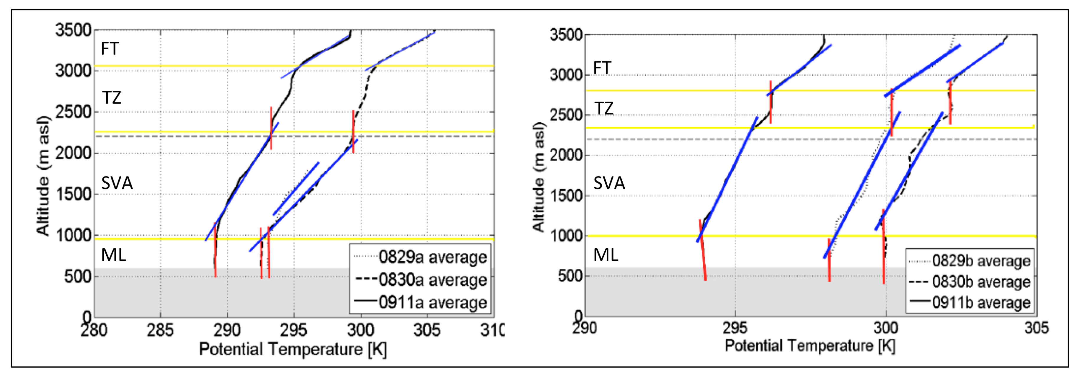
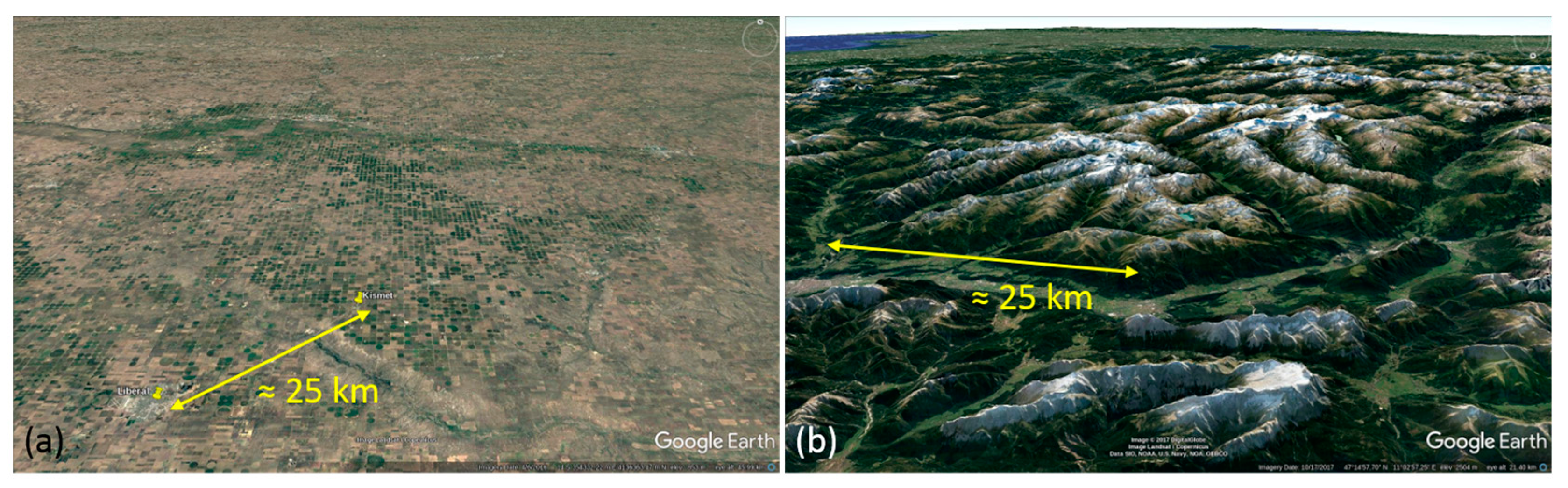
Table 1.
List of transport and exchange processes over mountainous terrain for momentum, energy, and mass. The references in columns 3–5 relate to studies in which specifically exchange of momentum, energy and mass has been studied or observed. The lists of references are non-exhaustive; no more than three references are shown for either process and exchange variable.
| Scale | Process | Momentum | Energy | Mass |
|---|---|---|---|---|
| Meso-α (mountain-range scale) | Mountain-plain circulation | [72] | [73] | [54,74] |
| Meso-β (mountain-range scale) | Gravity waves | [3,30,75] | [76,77] | [78,79] |
| Forced lifting | [80,81] | [82,83,84] | ||
| Meso-γ (mountain/valley scale) | Valley winds | [52,58,85] | [49,85] | [52,86,87] |
| Flow channeling | [88,89] | [86] | ||
| Rotors/wave breaking | [61,90] | [91,92] | [91] | |
| Boundary-layer gravity waves | [93,94,95] | |||
| Micro-α (slope scale) | Slope winds | [58,96,97] | [31,34,69] | [44,98,99] |
| Valley subsidence | [100,101] | [43,69,102] | [103,104] | |
| Moist convection | [105,106] | [105,106] | [107,108,109] | |
| ≤ Micro-β (turbulent scale) | Turbulent transport | [110,111] | [69,112,113] | [101,114] |
| Radiation | - | [58,115] | - |
© 2018 by the authors. Licensee MDPI, Basel, Switzerland. This article is an open access article distributed under the terms and conditions of the Creative Commons Attribution (CC BY) license (http://creativecommons.org/licenses/by/4.0/).
Share and Cite
MDPI and ACS Style
Lehner, M.; Rotach, M.W. Current Challenges in Understanding and Predicting Transport and Exchange in the Atmosphere over Mountainous Terrain. Atmosphere 2018, 9, 276. https://doi.org/10.3390/atmos9070276
AMA Style
Lehner M, Rotach MW. Current Challenges in Understanding and Predicting Transport and Exchange in the Atmosphere over Mountainous Terrain. Atmosphere. 2018; 9(7):276. https://doi.org/10.3390/atmos9070276
Chicago/Turabian StyleLehner, Manuela, and Mathias W. Rotach. 2018. "Current Challenges in Understanding and Predicting Transport and Exchange in the Atmosphere over Mountainous Terrain" Atmosphere 9, no. 7: 276. https://doi.org/10.3390/atmos9070276
Note that from the first issue of 2016, this journal uses article numbers instead of page numbers. See further details here.