Magnetic Biomonitoring as a Tool for Assessment of Air Pollution Patterns in a Tropical Valley Using Tillandsia sp.

Abstract

Recently, air pollution alerts were issued in the Metropolitan Area of Aburrá Valley (AVMA) due to the highest recorded levels of particulate matter (PM_2.5 and PM₁₀) ever measured. We propose a novel methodology based on magnetic parameters and an epiphytic biomonitor of air pollution in order to improve the air pollution monitoring network at low cost. This methodology relies on environmental magnetism along with chemical methods on 185 Tillandsia recurvata specimens collected along the valley (290 km²). The highest magnetic particle concentrations were found at the bottom of the valley, where most human activities are concentrated. Mass-specific magnetic susceptibility (χ) reaches mean (and s.d.) values of 93.5 (81.0) and 100.8 (64.9) × 10⁻⁸ m³ kg⁻¹ in areas with high vehicular traffic and industrial activity, while lower χ values of 27.3 (21.0) × 10⁻⁸ m³ kg⁻¹ were found at residential areas. Most magnetite particles are breathable in size (0.2–5 μm), and can host potentially toxic elements. The calculated pollution load index (PLI, based on potentially toxic elements) shows significant correlations with the concentration-dependent magnetic parameters (R = 0.88–0.93; p < 0.01), allowing us to validate the magnetic biomonitoring methodology in high-precipitation tropical cities and identify the most polluted areas in the AVMA.

1. Introduction

Magnetic biomonitoring studies have gained importance in the field of environmental magnetism in the last two decades, mainly because this technique has been used as a tool to study the changes in the pollution load in specific environments, such as urban areas, through magnetic measurements in a wide range of natural materials [1,2]. Concerning atmospheric pollution, some authors have demonstrated the importance of magnetic biomonitoring for determining particulate matter pollution levels in several cities in Central and South America [3,4,5].

Most of the magnetic minerals in airborne particulate matter (PM) and total suspended particles (TSP) come from human activities, termed anthropogenic. PM_2.5, PM₁₀, and TSP can be deposited and accumulated in biological surfaces such as lichens, mosses, and tree leaves. When magnetic minerals, elements, polycyclic aromatic hydrocarbons (PAHs), polychlorinated biphenyls (PCBs), etc. of such deposited/accumulated particles are quantified; and these organisms present visible morphological changes, they are called bioaccumulators or biomonitors [6]. The characterization of minerals as magnetite, hematite, maghemite, products of fuels burning, or products of brake-linings, road surface, and tire wear, could convey valuable information about air quality in places where biomonitors have been growing or transplanted [7,8,9,10]. Additionally, the implementation of lichens, mosses, and tree leaves as biomonitors is useful compared with traditional monitoring mechanisms due to the low cost and quick analysis [5,11,12,13,14,15,16,17].

The use of organisms to assess environmental impact is relatively widespread. Bioindicators and biomonitors of environmental impact are used for the purpose of observing changes in biological processes and the state of communities or species. Indeed, bioindication and biomonitoring techniques are starting to be used in legal action (e.g., in Europe) because their relevance has already been recognized by international committees (e.g., for lichens, mosses, and tobacco plants). The terms biomonitoring and bioindication refer to specific uses. Bioindicators assess biotic response to environmental stress qualitatively. For instance, the presence, reduction, or absence of a species from the environment may be a bioindicator. Good indicators are common and abundant; their ecology and physiology are well understood, and they are sensitive to environmental stress. For example, exposure to pollutants may result in unspecific reactions by a particular species, which may allow us to recognize a polluted site and an unpolluted site. Passive bioindicators are recognized as biomonitors. Tillandsia recurvata L. is a good biomonitor because it is widespread and is an effective accumulator of pollutants.

T. recurvata L. is an epiphytic plant from the Bromeliaceae family that usually tends to create a spheroidal shape and has a basic root system. These plants have foliar trichomes that allow the absorption of water, nutrients, and dust from the air [18]; since they can colonize trees and cables, they are available and well distributed in the Aburrá Valley (Colombia). Out of all vascular plants, these species are considered to be the most tolerant to stress. The Tillandsia spp. have a high efficiency of water economy, well-developed support structures, and the ability to obtain mineral nutrients from very diluted resources such as rainwater. The absorption of minerals takes place when the buds are wet immediately after rain. Tillandsia spp. are widely distributed in America and many of the islands of the West Indies. These characteristics facilitate the study of their capacity as accumulator of different pollutants, such as toxic elements, particles, and magnetic minerals [3].

Properties of T. recurvata and T. capillaris as magnetic biomonitors of atmospheric pollution have been reported by [3] in Querétaro metropolitan area (México) and by [4] in Córdoba province (Argentina), respectively. Climatic conditions in those areas are different from AMVA, e.g., the average annual temperature in Querétaro is 18 °C and it has around 60 days a year with rain. The biomonitor’s qualities for retaining airborne PM from the environment, even in rainy weather conditions, are prominent. This species is not cleaned by rain; on the contrary, it retains more pollutants when it is wet. In the Metropolitan Area of Aburrá Valley this epiphyte is abundant all along the valley, except in locations exceeding 2000 meters above sea level, where it is scarce or absent. Nevertheless, T. usenoides seems to be present at these locations.

Schrimpff [19] conducted the first biomonitoring study in the Aburrá Valley in Colombia with T. recurvata, assessing heavy metals, PAHs, and chlorinated hydrocarbons. This author obtained concentration maps and discussed the possible sources of these airborne compounds. Recent studies have used T. usenoides as an active monitor (using transplants) of heavy metals [20], and later studies have used lichens at some air quality monitoring stations (REDAIRE) with the aim of determining air quality [21].

Given the adverse effect of PM_2.5 and PM₁₀ on human health, people living in highly contaminated cities are more prone to developing breathing and cardiovascular diseases, asthma [22,23], and possibly mental disorders [24]. In this sense, the implementation of additional methodologies to the regular air quality monitoring would be necessary to determine vulnerable places in extensive areas such as the AVMA.

The main goal of this study is to assess the airborne PM impact on an extensive and densely populated area through: (a) the characterization of magnetic particles present in collected samples; (b) the use of multivariate statistical methods on magnetic and chemical variables in order to identify relevant magnetic parameters as potential pollution indicators; and (c) the detection of the most polluted sites in the AVMA.

2. Experiments

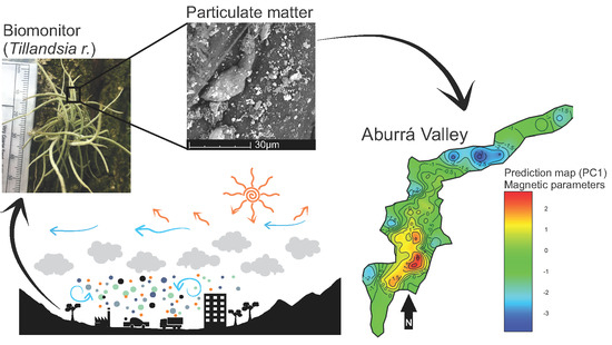
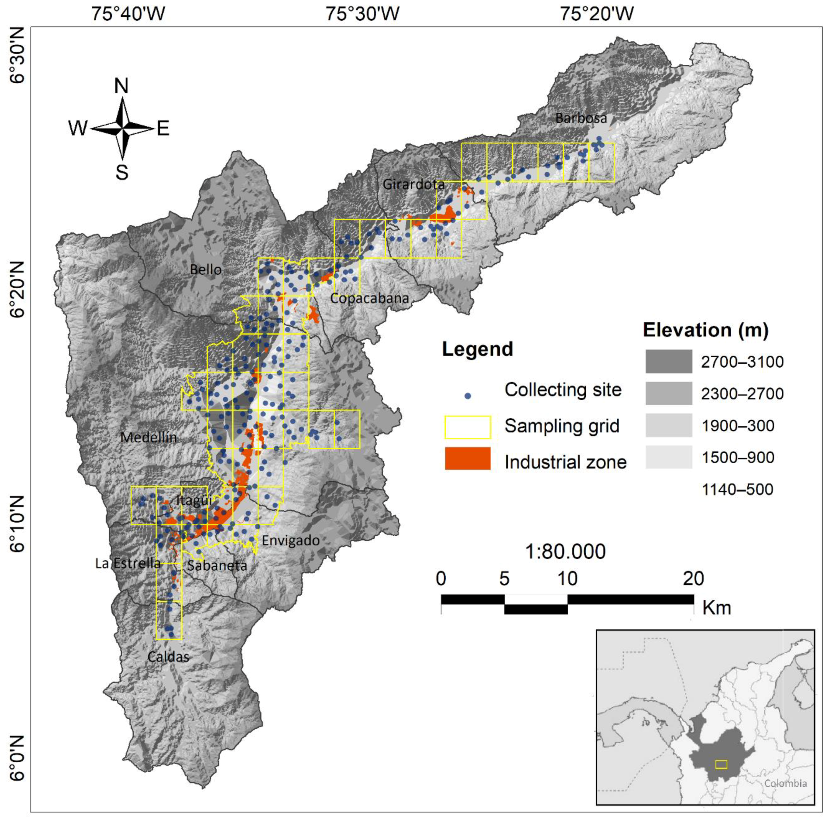
2.1. Study Area

The Aburrá Valley (a Colombian inter-Andean basin), is a N–S straight valley of 24 km in length and 12 km wide. It is surrounded by mountains that rise up to 1000 m above the bottom of the valley. The Aburrá Valley metropolitan area corresponds to a conglomerate of 10 municipalities, whose most populated entity is Medellín (Figure 1). According to [25], AVMA had about 3.8 million inhabitants in 2016, concentrated in an 1157 km² area, reaching 22.681 inhabitants per km².

Emission inventories from AMVA assign 59% of PM_2.5 to vehicle-derived traffic from a fleet of 1.2 million of vehicles (motorcycles, cars, taxis, buses, and trucks), and an additional 34% of PM_2.5 is attributed to industrial sources located mostly in the center of the valley [26].

The AVMA has tropical weather, where rainfall is mostly controlled by trade winds, defining two rainy seasons in the year (April and October). Annual precipitation in the northern part of the valley is ~1400 mm/year and ~3000 mm/year in the south [27]; such meteorological conditions are ideal for the accumulation of gases and PM during cloudy periods, occurring mostly between March and April, when sun radiation cannot reach the valley floor to heat the air, preventing air from rising and dispersing the air pollutants. The wind regime inside the Aburrá Valley is dominated by pressure canalization along the valley axis, marked by the Medellín River. During the day, the higher pressure to the north pushes the wind from north to south (up the valley), coupled with anabatic winds that push the wind upward from the bottom of the valley. During early night, katabatic winds dominate, moving the air down the hill and then down the valley (south to north) [28].

2.2. Sampling

A total of 185 samples of T. recurvata were collected in September 2016 from AVMA urban areas. The sampling campaign was performed with predominantly sunny weather, and all samples were collected over a period of four weeks, which minimized the climate variability during sample collection. Regardless, Tillandsia recurvata has an advantage over tree leaves in that even heavy rains do not seem to wash away the accumulated particles [3]. A sampling grid was designed in order to divide the metropolitan area into 50 squares of 6 km² (Figure 1). Each site was selected according to epiphyte availability and following the methodology proposed by [3]. Samples were taken in residential, vehicular, and industrial areas, from trees located along avenues and secondary streets. Vehicular areas were identified as zones (avenues and freeways) used preferentially by regular traffic to travel between industrial and residential areas, or between different residential areas. These areas are affected by traffic, which commonly follows a stop-and-go pattern, resulting in increased brake and road wear. The size of each specimen of T. recurvata was controlled in order to collect samples with similar conditions and temporality, choosing individuals of T. recurvata of about 10–15 cm diameter. A minimum collection height of 1.5 m was used in order to avoid, as much as possible, the influence of re-suspended soil particles.

Additionally, in order to obtain a baseline value, three individual control samples were collected from the city outskirts in a forest area with minimum anthropogenic particle contribution. Samples were carefully collected using latex gloves and non-magnetic tools to avoid contamination and stored in paper bags. Samples were then dried in a laboratory furnace at 40 °C in order to avoid mineralogical transformation. The dried plants were crushed using a hand grinder with a ceramic finish. Grinded material was packed in plastic containers of 8 cm³, and firmly pressed to prevent movement during magnetic measurements.

2.3. Magnetic Measurements

Magnetic measurements were carried out at the Laboratory of Magnetism and Paleomagnetism at the CIFICEN-IFAS-UNCPBA (Argentina) and the Environmental Magnetism and Paleomagnetism Laboratory at EAFIT University (Colombia). Magnetic susceptibility (κ, volume) was measured using a MS2 susceptibilimeter from Bartington Instruments Ltd. (Witney, England), linked to a MS2B dual frequency sensor (0.47 and 4.7 kHz). Replicate measurements were done for each sample on the higher sensitivity range (0.1 × 10⁻⁵ SI); moreover, κ values were corrected for drift through five measurement cycles (two air readings and three sample readings). The accuracy of the measurement of κ is 1%. Mass-specific magnetic susceptibility parameter χ was calculated using the κ measurements and sample weight. Anhysteretic remanent magnetization (ARM) was imparted to all samples using a device coupled with an alternating field (AF) demagnetizer (Molspin Ltd.), superposing a DC bias field of 50 and 90 µT to a peak AF of 100 mT and at AF decay rate of 17 µT per cycle. The remanent magnetization was measured using a spinner fluxgate magnetometer Minispin (Molspin Ltd., Newcastle upon Tyne, Tyne and Wear, England), which has a noise level <2.5 × 10⁻⁵ A/m and a sensitivity of 10⁻⁴ A/m. Such measurements were used to determine the mass-specific ARM (at DC = 71.58 A/m) and the anhysteretic susceptibility (mass-specific χ_ARM), using a linear regression with different DC values (39.78 and 71.58 A/m). The χ_ARM/χ and the King’s Plot (χ_ARM vs. χ), from [29] were also constructed. Isothermal remanent magnetization (IRM) measurements were performed using an ASC Scientific Pulse Magnetizer (Narragansett, RI, USA) model IM-10-30. Samples were magnetized in 27 steps, by exposing each sample to increasing fields from 1.7 mT to 2470 mT. The IRM was measured using the abovementioned magnetometer. IRM saturation (SIRM) was determined at a field of 2470 mT. The remanent coercivity (H_cr), and S-ratio (=−IRM_-300mT/SIRM) were obtained by applying a reverse field once the SIRM was reached.

2.4. Chemical Analysis and Microscopy Observations

The elements V, Cr, Co, Ni, Cu, Zn, Mo, Sn, Sb, Ba, Pb, and Fe were determined in 51 selected samples by inductively coupled plasma optical emission spectrometry (ICP-OES), using a Shimadzu 9000 (Kyoto, Japan) (simultaneous high-resolution, norm EPA 200.7) at the Laboratory of Chemical Analysis (LANAQUI, CERZOS-CONICET-UNS, Argentina). Each sample (~1 g of pulverized material) was dried in an electronic controlled stove under 40 °C for 24 h, and then sieved in order to eliminate major impurities. The samples were digested in ultrapure grade nitric acid (SW 846-US EPA 3051) using a MARS-5 microwave digestion system at 800 W, 350 psi and 170 °C for 10 min. The analysis was performed using the high-resolution ICP-OES Shimadzu 9000 with a torch injector (Glass Expansion, Port Melbourne, Australia). Reported data correspond to an average value after measurements on two independent replicated samples, all of them within a standard deviation <2.5%. Data were obtained using a double methodology: (1) external aqueous calibration and (2) evaluation/correction of drifting and interferences using standard addition. All standards used were certified by the B-8210, Chem-Lab (Zedelgem, Belgium) and Milli-Q (EMD Millipore, Burlington, MS, USA) water at 0.05 mS/cm and 18.2 MΩ/cm at 25 °C. In order to determine the accuracy of the methodology, the same protocol was applied on a Certified Reference Material: “Trace Elements on Fresh Water Sediment”, Catalog Nr. CNS 392-050, Lot. Nr. 011295 (Dutch Centre for Water Management, Resource Technology Corporation, Laramie, WY, USA). Once the data of recovery (percent) for every tested element were determined, the original sample results (obtained by double analytical methodology) were corrected by using a correction factor. Detection limits for each element are: 0.05 mg/kg (Co); 0.02 mg/kg (Cr); 0.04 mg/kg (Cu); 0.01 mg/kg (Fe); 0.05 mg/kg (Mo); 0.03 mg/kg (Ni); 0.04 mg/kg (Pb); 0.02 mg/kg (V); 0.01 mg/kg (Zn); 0.03 mg/kg (Sn); 0.03 mg/kg (Sb); and 0.01 mg/kg (Ba).

The pollution index (PLI, [30]), a composite index based on 11 potentially toxic elements (PTE), V, Cr, Co, Ni, Cu, Zn, Mo, Sn, Sb, Ba, and Pb, was calculated for 50 samples using Equation (1):

$$PLI=\sqrt[n]{{\displaystyle \prod }_{i=1}^n\left(\frac{C_{HM},i}{C_{base},i}\right)}$$

(1)

where C_HM,i is the concentration of each PTE, and C_base,i is the baseline value for each element. Such values (Supplementary Materials, Table S2) were obtained from a control sample with minimum influence of pollution.

Samples of T. recurvata were examined by scanning electron microscopy (SEM), using a Phillips microscope model XL30 (ThermoFisher, Waltham, MA, USA). This microscope also allowed us to analyze the elemental composition of single particles by X-ray energy dispersive spectroscopy (EDS) with an EDAX (Berwyn, PA, USA) model DX4 (detection limit 0.5%).

2.5. Statistical Analysis

To analyze the relationship between magnetic parameters and PTE chemistry, a principal component analysis (PCA) with matrix correlation was analyzed. Before applying this analysis, a multi-normality analysis was performed. In order to fit it, transformations to multi-normality of [31] were applied.

Groups of samples were built based on the principal components coordinates accumulated over 80% of variance, ensuring that the dataset representation is adequate. The fuzzy clustering analysis (FC) was performed in order to build these groups. The main difference between FC and the classical clustering method lies in the possibility that a sample belongs to more than one cluster in the FC method. In the FC method, each sample is assigned a membership value for all clusters as degrees in the interval (0,1). Furthermore, these membership degrees offer finer detail to the data model [32]. This method is applied in order to determine features along sample transitions between extreme clusters. The PLI values of the FC were calculated and contrasted with magnetic variables values.

Based on a previous analysis and looking to show potentially polluted and less polluted sites, the Ordinary Kriging method (OK) was used to build a prediction map of the most relevant magnetic parameters and index PLI. The OK is the most popular interpolation spatial method because it considers knowledge of the spatial variation as represented in the variogram function, and does not require additional information than the measurement values and their geographic coordinates. The statistical analyses were performed using the R free software (Vienna, Austria, R version 3.4.0, 2017).

3. Results and Discussion

3.1. Magnetic Properties

Magnetic parameters and related ratios were determined for all samples. They can be described as magnetic concentration (χ, ARM and SIRM), magnetic mineralogy (H_cr, S-ratio) and magnetic grain size (SIRM/χ, χ_ARM/χ and ARM/SIRM) dependent parameters. Such parameters are detailed in the Supplementary Materials (Table S1).

According to [33], the magnetic susceptibility parameter roughly approximates the concentration of magnetic particles in a given sample. Measured χ values varied from 0.1 to 372.9 × 10⁻⁸ m³ kg⁻¹ (Figure 1). The highest concentrations of magnetic particles correspond to sampling sites where land use was classified as industrial (I) and vehicular (V), with mean values of 100.8 and 93.5 × 10⁻⁸ m³ kg⁻¹, respectively; while residential (R) areas dominantly show lower mean values of 27.3 × 10⁻⁸ m³ kg⁻¹ (

Table 1. Descriptive statistics of residential, industrial, and vehicular areas. Magnetic concentration- and mineralogy-dependent parameters, elemental concentration, and pollution index PLI.

Samples	Χ (10−8 m3 kg−1)		ARM (10−6 A m2 kg−1)		SIRM (10−3 A m2 kg−1)			Hcr (mT)			S-ratio (a.u.)		SIRM/χ (kA/m)		χARM/χ (a.u.)		ARM/SIRM (a.u.)
Residential (n = 91)
min	0.1		2.9		0.3			26.2			0.90		5.5		0.9		0.009
max	88.8		141.8		8.5			40.3			1.00		23.7		10.8		0.023
mean	27.3		38.4		2.5			34.2					10.7		2.1		0.015
s.d.	20.9		24.8		1.6			2.8					3.1		1.2		0.002
Industrial (n = 22)
min	19.7		25.2		2.0			32.5			0.91		6.7		0.6		0.011
max	267.9		282.1		21.7			42.7			1.00		13.5		2.2		0.016
mean	100.8		121.7		9.5			36.4					9.7		1.5		0.013
s.d.	64.9		73.2		5.9			2.4					1.8		0.4		0.001
Vehicular (n = 69)
min	6.2		14.1		0.9			23.8			0.83		5.1		0.4		0.012
max	372.9		353.0		25.0			42.1			1.00		14.7		2.7		0.019
mean	93.5		101.4		7.1			35.6					8.3		1.5		0.015
s.d.	81.0		74.6		5.4			3.8					1.7		0.4		0.001
Control (n = 3)
min	2.1		7.7		0.5			33.6			0.91		12.4		2.5		0.015
max	6.6		13.3		0.8			34.2			0.97		23.8		5.0		0.016
mean	4.3		10.8		0.7			33.8					17.7		3.3		0.016
s.d.	2.2		2.9		0.2			0.3					5.7		1.4		0.001
Samples	Ba	Co	Cr	Cu		Fe	Mo		Ni	Pb		Sb		Sn		V		Zn	PLI
	(mg/kg)	(mg/kg)	(mg/kg)	(mg/kg)		(mg/kg)	(mg/kg)		(mg/kg)	(mg/kg)		(mg/kg)		(mg/kg)		(mg/kg)		(mg/kg)	(a.u.)
Residential (n = 19)
min	26.0	0.11	5.3	7.0		8.0	0.2		2.0	2.0		0.9		0.0		1.2		41.0	0.8
max	158.0	8.00	193.0	47.0		183.0	1.2		105.0	38.0		5.6		7.9		19.0		255.0	5.3
mean	80.6	1.24	35.4	19.8		47.1	0.5		15.6	9.7		2.2		1.6		7.8		119.1	2.2
s.d	41.4	1.73	42.0	11.9		37.1	0.3		22.8	8.9		1.2		1.8		4.7		67.1	1.2
Industrial (n = 8)
min	88.0	0.08	20.0	17.0		30.0	0.4		8.0	10.0		2.0		0.9		5.2		86.0	2.0
max	549.0	1.00	122.0	100.0		189.0	2.5		35.0	60.0		9.9		12.0		30.0		577.0	6.9
mean	276.3	0.57	48.1	54.6		85.5	1.6		18.3	27.0		5.9		6.9		15.4		302.4	4.9
s.d	159.9	0.30	33.0	32.6		48.0	0.7		8.5	18.4		2.7		4.1		7.4		166.5	1.8
Vehicular (n = 23)
min	72.0	0.08	9.4	14.0		18.0	0.4		5.0	2.0		0.2		0.7		2.8		71.0	1.8
max	505.0	4.30	174.0	209.0		181.0	6.3		80.0	70.0		20.0		46.0		33.0		333.0	10.7
mean	241.6	0.93	65.6	59.3		87.0	1.6		23.0	24.2		6.4		8.9		13.6		210.5	4.7
s.d	130.3	1.18	39.5	45.9		43.0	1.4		15.9	19.2		4.6		10.9		7.1		77.1	2.1

). ARM and SIRM parameters indicate a wide variation in concentration of ferrimagnetic minerals that are mainly derived from anthropogenic sources in the AVMA. Minimum and maximum values vary from 2.9 to 353.0 × 10⁻⁶ A m² kg⁻¹ for ARM, and from 0.3 to 25.0 × 10⁻³ A m² kg⁻¹ for SIRM.

The variability of concentration for the magnetic dependent parameters in relation to different land uses found in the AVMA is comparable to 38 Indian cities studied by [34], where these authors reported that the magnetic properties of airborne dust particles collected in artificial containers reported significant differences between R, V, and I areas. Figure 2a shows different IRM acquisition curves for samples chosen from R, V, and I areas; the saturation is almost always reached at ~300 mT, showing the predominance of ferrimagnetic particles [35]. Some samples from industrial areas do not seem to reach saturation at such fields, indicating the possible contribution of high-coercivity minerals such as hematite. Despite the acquisition curves not revealing marked mineralogical differences, the SIRM values for samples V and I are higher with respect to samples R, thus denoting a higher concentration and accumulation of ferrimagnetic minerals on T. recurvata for these studied sites.

The H_cr values indicate the presence of magnetite-like minerals [35]. According to land use, the mean H_cr (s.d.) values vary in a narrow range, e.g., 34.2 (2.8) mT (R), 35.6 (3.8) mT (V) and 36.4 (2.4) mT (I). Complementary to H_cr, the S ratio is widely used in order to assess the relative contribution of ferrimagnetic versus antiferromagnetic minerals [36]. Obtained S ratio values evidence the predominance of low-coercivity phases, with most of values ranging between 0.95 and 1. Although magnetic mineralogy in the AVMA is dominated by ferrimagnetic minerals, higher mean values of H_cr may indicate the presence of high-coercivity minerals [37,38] for different land use areas (Table 1) and such mineral contribution to the IRM is smaller in residential than vehicular and industrial areas (Figure 2a).

The relative magnetic grain-size distribution, inferred from a correlation of χ and χ_ARM parameters (King’s Plot) is presented in Figure 2b. Most of the analyzed samples are dominated by particles with magnetic grain-size between 1 and 5 μm, without a strong bias due to land use (Figure 2b). However, accumulated particles in residential areas and the control site tend to be dominated by finer magnetic grain sizes (about 1 μm). Moreover, magnetic grains smaller than 1 μm are mostly present in residential areas located on the AVMA slopes, where usually less vehicular and industrial activity is present. This behavior is also evidenced by the inter-parametric ratios χ_ARM/χ, SIRM/χ and ARM/SIRM. In these cases, the mean values of such ratios are higher (indicating finer magnetic grains) for residential and control areas compared to other land use areas (Table 1). The correlation between a concentration parameter (SIRM) and a magnetic grain size dependent parameter (χ_ARM/χ), shows that the magnetic grain size increases in sites with higher SIRM values (SIRM > 9.5 × 10⁻³ A m² kg⁻¹), while lower SIRM values tend to have smaller magnetic grain size, i.e., higher values of χ_ARM/χ (Figure 2c).

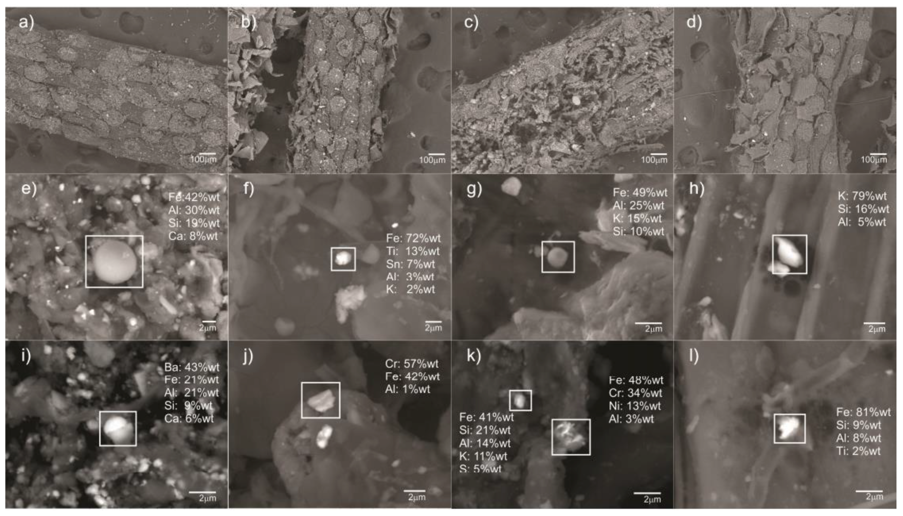
3.2. SEM/EDS and Elemental Analysis

In order to characterize their morphology and quantify the elemental composition by EDS, selected samples, considered representative from the control and three land use areas, were observed under SEM.

Specimens of T. recurvata L. collected from all determined land uses (industrial, vehicular, residential sites and the control areas, Figure 3a–d, respectively) show clear differences in their leaves and general aspect.

Iron-rich particles are present at all sites; however, their presence and size increase in the following order: residential area < vehicular area < industrial area. Forty-nine characteristic spherules, semi-spherules and irregular Fe-rich particles from 0.3 to 6.6 μm were identified; some of such particles are shown in Figure 3e–l. Analyzed particles were also revealed to have higher sizes in industrial areas (mean size = 2.9 μm; n = 20) than in vehicular areas (mean size = 1.2 μm; n = 12) and residential areas (mean size = 1.7 μm; n = 12).

Iron-oxide-rich spherules are common components of the PM_2.5, PM₁₀, and TSP emitted from industrial sites, especially from metallurgical factories, as reported by Chaparro et al. [14]. In the present study, ~67% of the particles analyzed under SEM were spherules of 0.8–6.4 μm, with a mean size of ~2.7 μm. Figure 3 gathers some of the most common particle morphology observed in areas with different land usages: (a) Industrial areas are characterized by perfect iron-oxide spherules with different sizes (Figure 3e,i; 6.4 μm and, 2.3 μm respectively); (b) Vehicular areas are characterized by irregular (Figure 3j) and semi-spherical (Figure 3f) particles, where irregular particles range from 0.3 to 3.1 μm with mean size = 1.2 μm (n = 10); (c) Residential areas are characterized by semi-spherical and irregular particles ranging from 0.5 to 4.5 μm and mean size of 1.5 μm (n = 9) (Figure 3g,k); (d) Control sites are characterized by irregular particles ranging from 1 to 2.1 μm in size (Figure 3h,l). Whole-sample quantitative chemical analysis, using ICP-OES and SEM/EDS semi-quantitative chemical analysis, were performed on selected samples in order to characterize both the total elemental contents and the chemical composition of discrete particles in samples from different land usage sites.

Elemental composition of whole samples from 51 sites was performed by ICP-OES. Results are listed in the Supplementary Materials (Table S2) and their corresponding descriptive statistics are shown in Table 1. Most of the elements detected by EDS analysis were then confirmed by ICP-OES (Table 1, Figure 3). In addition, the ICP-OES data show a significant correlation between the simultaneous appearance of Fe and V (R = 0.700, p < 0.01), Fe and Cr (R = 0.635, p < 0.01), Fe and Ni (R = 0.557, p < 0.01), and Fe and Pb (R = 0.546, p < 0.01) (

Table 2. Pearson’s coefficients (R-values) for correlations between magnetic and chemical variables from T. recurvata samples AMVA (n = 50).

Variable	χ	ARM	SIRM	Hcr	SIRM/χ	χARM/χ	ARM/SIRM	Ba	Co	Cr
χ	1
ARM	0.955 **	1
SIRM	0.939 **	0.991 **	1
Hcr	0.341 *			1
SIRM/χ	−0.474 **	−0.386 **	−0.346 *	−0.382 **	1
χARM/χ	−0.460 **	−0.394 **	−0.384 **	−0.300 *	0.844 **	1
ARM/SIRM			−0.370 **				1
Ba	0.880 **	0.859 **	0.846 **	0.499 **	−0.449 **	−0.423**		1
Co				−0.618 **					1
Cr	0.641 **	0.698 **	0.678 **					0.494 **	0.576 **	1
Cu	0.880 **	0.752 **	0.725 **	0.484 **	−0.467 **	−0.438 **		0.814 **		0.424 **
Fe	0.785 **	0.824 **	0.819 **		−0.295 *	−0.354 *	−0.318 *	0.521 **		0.635 **
Mo	0.897 **	0.780 **	0.750 **	0.485 **	−0.434 **	−0.403 **		0.808 **		0.432 **
Ni	0.440 **	0.539 **	0.526 **	−0.416 **				0.285 *	0.775 **	0.930 **
Pb	0.645 **	0.667 **	0.666 **		−0.302 *	−0.280 *		0.604 **		0.673 **
Sb	0.828 **	0.678 **	0.641 **	0.506 **	−0.539 **	−0.462 **		0.748 **		0.348 *
Sn	0.827 **	0.668 **	0.633 **	0.461 **	−0.401 **	−0.341 *		0.713 **		0.337 *
V	0.686 **	0.744 **	0.752 **			−0.314 *	−0.388 **	0.686 **		0.630 **
Zn	0.588 **	0.653 **	0.658 **	0.391 **	−0.303 *	−0.302 *		0.686 **
PLI	0.933 **	0.905 **	0.880 **	0.323 **	−0.487 **	−0.451 **	−0.192 *	0.891 **		0.693 **
Variable	Cu	Fe	Mo	Ni	Pb	Sb	Sn	V	Zn	PLI
Cu	1
Fe	0.449 **	1
Mo	0.953 **	0.479 **	1
Ni		0.557 **		1
Pb	0.521 **	0.546 **	0.481 **	0.549 **	1
Sb	0.895 **	0.283 *	0.913 **		0.398 **	1
Sn	0.938 **	0.390 **	0.960 **		0.393 **	0.918 **	1
V	0.541 **	0.700 **	0.539 **	0.498 **	0.616 **	0.317 *	0.422 **	1
Zn	0.515 **		0.543 **		0.411 **	0.514 **	0.438 **	0.43 **	1
PLI	0.868 **	0.785 **	0.869 **	0.510 **	0.737 **	0.807 **	0.778 **	0.670 **	0.677 **	1

significant at the 0.05 level (*) and at the 0.01 level (**).

). Irregular iron-rich particles coupled with chromium and nickel, as well as metallic iron, were identified along vehicular and residential areas, showing fine and ultra-fine phase sizes. These are associated with metal structures’ wear and corrosion (due to weather exposure and friction), as well as autoparts’ wear. Iron oxide particles associated with chromium and zinc were found in vehicular (Figure 3f,j) and residential areas (Figure 3g,k). In addition, particles composed of iron oxide, chromium, and nickel were found in samples from residential areas (Figure 3g,k). Spheroidal iron oxide particles are often associated with casting and welding processes performed in the industry in the study area, e.g., iron oxide spherules observed in Figure 3e,i correspond to a site (TM14) close to a metallurgical factory.

Control samples also showed the presence of iron-rich particles. Some of these particles are coarse-sized (5 µm) and have euhedral mineral morphologies. Fine-grained irregular particles (mean size = 1.2 μm; n = 5) with similar composition were also found in the control site and may be interpreted as anthropogenic (titano) magnetite or ash derived (Figure 3l).

Elemental contents of Pb, Cr, V, Sn, Sb, Ba, Cu, Zn, and Mo measured on Tillandsias spp. in the Aburrá Valley (this work) are slightly different from those reported in Medellín city by [19]. New data, based on 51 selected samples (Table 1 and Supplementary Materials, Table S2), show higher mean values for Cu and Pb, and lower values for Zn, Ni, and Cr regarding data reported by [19].

Significant correlation was found between simultaneous appearance of Ba and Cu (R = 0.814, p < 0.01), Ba and Mo (R = 0.808, p < 0.01), Ba and Sb (R = 0.748, p < 0.01), Ba and Fe (R = 0.521, p < 0.01), Ba and V (R = 0.686, p < 0.01), Ba and Zn (R = 0.686, p < 0.01), and Ba and Pb (R = 0.604, p < 0.01) (Table 2).

BaSO₄ particles of apparent mineral and anthropic type were identified. Because no local sources of natural barite are known, we assume that all BaSO₄ is resulting from pollution. Some of these particles, found in industrial and vehicular areas, show the cleavage and well-defined angles characteristic of barite. Barite is mainly used in the glass and pigment industries, as well as for various processes in the automotive sector. Barite is particularly produced by the wear and tear of braking systems [39,40]. Spherical particles of BaSO₄ (Figure 3i) were also found in industrial areas (Figure 3i).

3.3. Statistical Analysis and Land Use Areas

Descriptive statistics of magnetic variables and PLI relative to I, V, and R land use areas are listed in Table 1. A multiple pairwise comparison was performed after a Kruskal–Wallis test (Conover Inman test), in order to analyze the differences between magnetic values on these areas. The results of this test showed that there are significant differences (p < 0.01) between R and other land usages (I and V) for all the concentration-dependent magnetic parameters (χ, ARM and SIRM), H_cr (mineralogy) and, χ_ARM/χ (magnetic size grain). Such significant variation of magnetic parameters for different land use areas is comparable to the study reported by [34] in R, V, and I areas from India.

Additionally, in this study, the Conover Inman test was performed for PLI; results show that there are significant differences (p < 0.01) in PTE between R areas and I and V areas; nevertheless, there are no significant differences between I and V areas.

The PCA with correlation matrix was performed considering all magnetic parameters. Results and graphical representations are summarized in

Table 3. Summary of multivariate analysis of T. recurvata samples. Clusters with similar magnetic features obtained from fuzzy clustering analysis; and loading values from principal component analysis, the values in brackets correspond to the correlation with the principal component.

Variable	Fuzzy Clustering Analysis			Principal Component Analysis
	G1	G2	G3	PC1	PC2	PC3
N	I = 0 V = 6 R = 43	I = 6 V = 28 R = 37	I = 16 V = 32 R = 12
χ (10−8 m3 kg−1)	11.9	36.3	129.0	23.05 (0.95)	0.69 (0.01)	3.06 (0.03)
ARM (10−6 A m2 kg−1)	24.9	50.2	139.4	19.52 (0.81)	4.1 (0.04)	16.26 (0.15)
SIRM (10−3 A m2 kg−1)	1.6	3.3	10.2	20.23 (0.84)	7.94 (0.08)	8.44 (0.08)
Hcr (mT)	34.0	34.6	36.4	4.83 (0.2)	17.75 (0.19)	0.49 (0)
SIRM/χ (kA/m)	14.28	9.32	8.18	15.06 (0.62)	23.1 (0.24)	3.24 (0.03)
χARM/χ (a.u.)	2.72	1.73	1.38	14.05 (0.58)	6 (0.06)	25.37 (0.23)
ARM/SIRM (a.u.)	0.016	0.015	0.014	3.27 (0.14)	40.42 (0.43)	43.14 (0.39)
mean PLI (CV%) (a.u.)	1.207 (57.0)	2.386 (78.0)	5.291 (5.2)	--	--	--
PLI min–max (a.u.)	0.820–1.560	1.290–3.620	1.830–10.740	--	--	--

and in the Supplementary Materials (Figure S1). With the first three principal components it is possible to explain 87% of the observed variance. This high value of explained variance represents a good reduction of dimension and the high quality of the dataset representation. The PC1 is mainly defined by the concentration-dependent parameters χ, ARM, and SIRM, which show high positive correlation. The grain-size-dependent parameters (SIRM/χ and χ_ARM/χ) contribute both to PC2 and PC1. However, their proportional contribution is higher for PC1 than for PC2.

PC3 is only populated by grain-size-dependent parameter ARM/SIRM. Values of loading and correlation with PCs are summarized in Table 3. In this way, it is evident that PC1 represents mainly the concentration of magnetic minerals and grain size and PC2 and PC3 represent the magnetic mineralogy and grain size of samples.

After executing the PCA, a fuzzy clustering analysis was performed in order to build clusters of samples based on magnetic parameters only. The clustering was made using three principal components, based on the accumulated 87% of the dataset variance. The dataset was partitioned into three clusters, G1 (n = 49) G2 (n = 71), and G3 (n = 60). In this case, the Dunn coefficient was evaluated and its value was 0.62, indicating that there are some samples sharing characteristics of different groups. The normalized Dunn coefficient indicates how fuzzy the partition is. A value of Dunn coefficient close to 0 indicates a very fuzzy clustering, and a value close to 1 indicates a near-crisp clustering. The cluster G1 shows the lowest values in concentration-dependent magnetic parameters. This cluster has features related to the softer magnetic minerals and finer magnetic grain size of the dataset. It is important to note that most of the samples with membership values over 50% belong to residential areas (i.e., n = 43 out of 46), and G1 lack samples from industrial areas. On the other hand, cluster G3 presents the opposite features to G1. This group has the highest values in concentration, coarser grain size, and relatively higher-coercivity mineralogy (the highest value in the corresponding parameters). This cluster is mostly constituted of samples from industrial areas (16 out of 22), 32 samples of vehicular areas, and some from residential areas (12 samples). The cluster G2 is a mix of all areas and values in all magnetic parameters corresponding to intermediate values. The group is composed by six samples from industrial areas (corresponding to 27% of all samples from industrial areas), 37 residential samples, and 28 vehicular samples.

The clusters using PLI values were calculated as well; a statistical summary is shown in Table 3. The G1 has lower concentration, soft mineralogy, and finer magnetic grains; it has the lowest mean value of PLI of 1.207 (s.d. = 0.680). The G2 has an intermediate value of PLI of 2.386 (s.d. = 1.850). The cluster G3 has the highest value of concentration, with higher-coercivity mineralogy and coarser magnetic grains, and has the highest PLI value of 5.291 (s.d. = 0.273).

3.4. Magnetic Biomonitoring

Magnetic properties are well suited as proxies of pollution records [41], with high sensitivity combined with fast laboratory processing and easy sample preparation. Laboratory instruments are relatively low cost, and most measurements are non-destructive [42]. An increasing number of studies use magnetic parameters to assess the air quality in urban areas by means of available biomonitors, such as lichens [5,14], mosses [12,16,43], and Tillandsia spp. [3,4], among others. In this magnetic biomonitoring study, in situ growing individuals of T. recurvata, with similar sizes and hence ages, were collected and used. This allows for assessing the pollution load in an extensive area during a determined (but not defined) period of accumulation. In such a sense, it is recommended, in the future, to carry out “active” biomonitoring, i.e., transplanting individuals of T. recurvata from natural (unpolluted) areas and doing sampling/measurements on determined periods (months, years, etc.) of interest. Such active biomonitoring not only allows us to define the collection period, but also to assess changes in time in order to, for example, verify the change in situation after strong anthropic events taking place in the environment.

Although there are several magnetic parameters, concentration-dependent ones have been used to evaluate the pollution load in extensive areas, as demonstrated by [44] and others. Such magnetic parameters can be used as pollution proxies in urban areas if pollution sources (vehicles and industries) contribute with Fe-rich particles [9,45,46,47] and if there is a relationship between these particles and PTE.

The present work interprets most of the magnetic particles observed as pollutants coming from human activities such as industrial processes and vehicular traffic, which are being gathered in different areas of the AVMA, as observed from parameters χ, ARM, and SIRM (Figure 4). Such preferential accumulation areas seem to be related to the highly congested roads and industrial infrastructure.

Prediction maps displayed in Figure 4 were built using χ (concentration-dependent magnetic parameter), PC1 (concentration- and grain-size-dependent magnetic parameters, that is, χ, ARM, SIRM, SIRM/χ, and χ/χ_ARM; the first three variables make a higher contribution to the PC according to their loading values), and pollution index PLI as response variables. The selected variables are based on statistical results (Table 3) obtained by combining magnetic parameters and chemical determination of PTE content on each sample.

Constructed variogram functions are of exponential type and their parameters are summarized in Table 3. Figure 4 shows the distribution of χ, PC1, and PLI obtained for the region. It is necessary to emphasize that high values of PC1 correspond to areas with a high concentration of magnetic minerals and high values of PLI to areas with high contents of potentially toxic elements. These areas are represented by the G3 group from the FC analysis, corresponding to the highest concentration of magnetic minerals, relatively higher coercivity mineralogy, coarser magnetic grain sizes and higher pollution index PLI. On the contrary, the lowest values of PC1 correspond to the group G1.

The most polluted sites in the AVMA are located in the south of the valley (Itagüí and the southern part of downtown Medellin), characterized by increasing concentration-dependent magnetic parameters: χ (>150.0 × 10⁻⁸ m³ kg⁻¹), ARM (>183.8 × 10⁻⁶ A m² kg⁻¹), and SIRM (>14.0 × 10⁻³ A m² kg⁻¹), as well as pollution index PLI > 6. The emissions of industrial activities mixed with traffic-derived pollution contribute to higher concentrations of magnetic particles compared with other areas (Figure 4). The distribution of magnetic particles in the Aburrá Valley is marked by higher concentrations of magnetic particles in the valley floor plains, near the Medellin River (mean values of χ, ARM and SIRM are 74.6 × 10⁻⁸ m³ kg⁻¹, 85.5 × 10⁻⁶ A m² kg⁻¹, and 6.0 × 10⁻³ A m² kg⁻¹, respectively), while some residential areas located at higher elevations present lower concentration related parameters (mean values of χ, ARM and SIRM are 39.0 × 10⁻⁸ m³ kg⁻¹, 53.6 × 10⁻⁶ A m² kg⁻¹, and 3.7 × 10⁻³ A m² kg⁻¹, respectively). An exception to this result is “El Poblado,” an area located on the southwest flank of the valley. El Poblado is characterized by a stepped topography, the highest vehicular density per habitant in the valley, high vehicular flow, and reduced mobility. El Poblado not only has the highest values of magnetic susceptibility (mean value of χ = 175.0 × 10⁻⁸ m³ kg⁻¹), but also has the highest pollution index (PLI < 10) in the valley.

In municipalities with small urban centers located in the northern part of the valley (Copacabana, Girardota, and Barbosa), concentration values (Figure 4) are as low (χ < 30.0 × 10⁻⁸ m³ kg⁻¹) as those found at higher altitudes in Medellín and Envigado. In the southern extreme of the valley (Caldas and La Estrella), concentration-dependent magnetic parameters increase with respect to the north, which seems to be related to the high density of textile, chemical, and ceramic industries located in this area of the valley.

The spatial variation of magnetic grain-size-dependent parameters, such as χ_ARM/χ, SIRM/χ and ARM/SIRM, shows the dominant presence of finer magnetic particles at higher altitude in residential or less polluted areas of the valley. Meanwhile, the bottom of the valley is dominated by a higher concentration of coarser magnetic sized particles. However, most of these particles are in the breathable size range, between 0.2 and 5 μm (Figure 2b). PM_2.5 and PM₁₀ in this range are harmful for human health because of their ability to be inhaled and reach deep portions of the respiratory system such as the pulmonary alveoli, making these particles capable of interacting directly with the bloodstream. Recently, iron-bearing particles have been demonstrated to be transported and biologically accumulated in the human brain, via the olfactory bulb, and associated with neurodegenerative diseases such as Alzheimer’s disease [24].

In addition to the potential risk due to the abundance of fine magnetite particles, such minerals can host PTE such as V, Cr, Ni, Cu, Zn, Mo, Sn, Sb, Ba, and Pb. This is supported by significant correlations between the magnetic and chemical variables summarized in Table 2. Pearson’s coefficients are statistically significant at the confidence level 0.01 for concentration-dependent magnetic parameters and chemical variables, R = 0.60–0.90 p < 0.01. According to the R-values, some PTE have higher affinity to magnetic particles, in the order Mo > Cu > Ba > Sb > Sn > V > Pb > Cr (Table 2). PLI is a composite index based on these PTE that correlates significantly with concentration-dependent magnetic parameters, e.g., R = 0.933, p < 0.01 for χ-PLI (Table 2). In this sense, the spatial variation of magnetic particles concentration represents, to a greater extent, the air quality with relation to the particle composition and its dispersion in AVMA (Figure 4).

4. Conclusions

Biomonitoring of air quality in a tropical valley was carried out using Tillandsia recurvata as a novel bioindicator of air quality. This study provides an overview of air quality from AMVA conditions using magnetic properties as proxies for potentially toxic element concentration and particle size. Analysis and interpretation of magnetic properties allow us to reach the following conclusions:

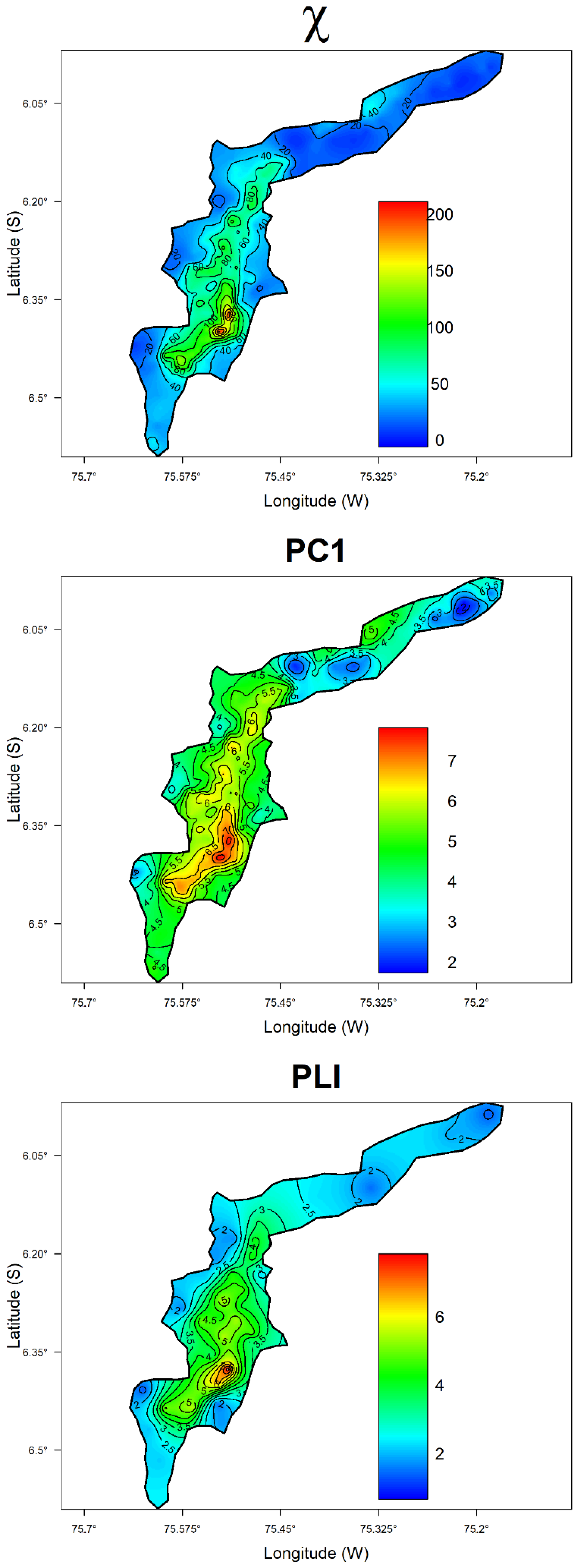
• The χ values vary in the range from 0.1 to 372.9 × 10⁻⁸ m³ kg⁻¹, reflecting very low to very high levels of air pollution in the AMVA. Variation in magnetic particle concentration estimated from susceptibility is characterized by χ values greater than about 100 × 10⁻⁸ m³ kg⁻¹ along the bottom of the valley, while residential areas on the valley slopes have lower values, of about 30 × 10⁻⁸ m³ kg⁻¹. Municipalities located on the northern part of the AVMA, such as Copacabana, Girardota, and Barbosa, display low magnetic concentration values. Similar values are only obtained in the residential suburbs of Medellín, located in the highest region of the hillside.
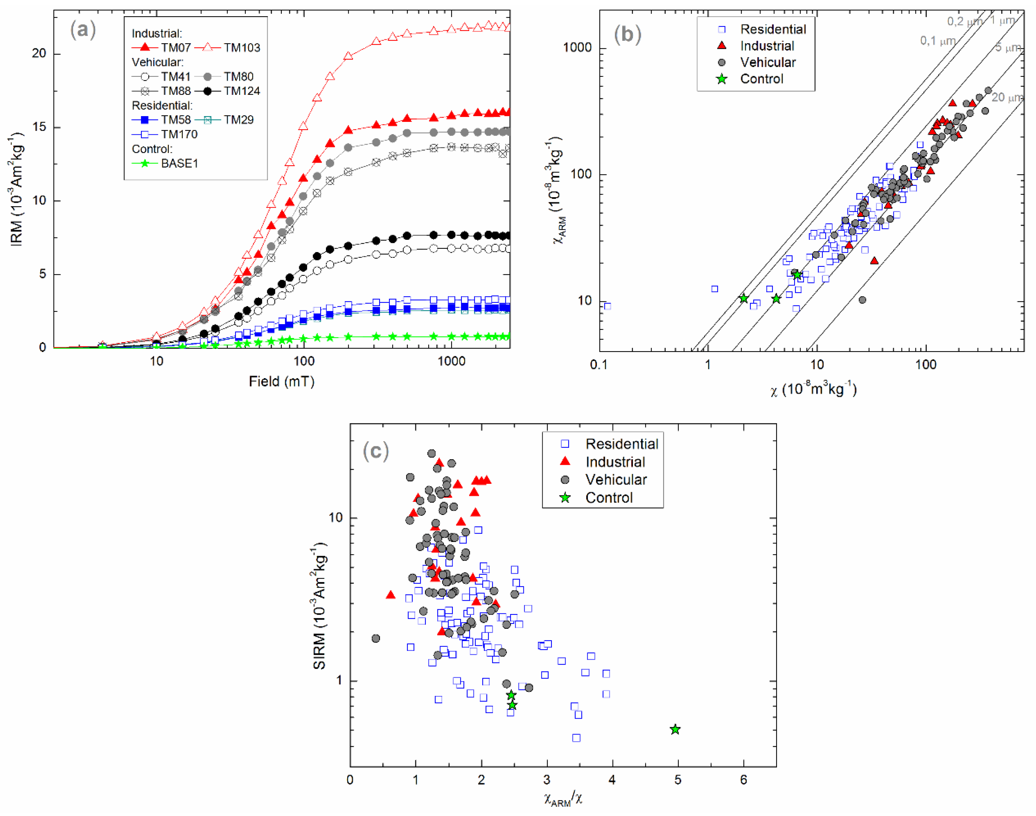
• Magnetic mineralogy as well as the magnetic susceptibility signal is dominated by ferrimagnetic phases of low coercivity, i.e., magnetite-like minerals, as indicated by IRM acquisition curves that reach saturation at fields of about 300 mT, and H_cr mean values of 34.2 mT for (R), 36.4 mT for (I), and 35.6 mT for (V) areas.
• Average magnetic grain size estimated from magnetic parameters (χ_ARM versus χ, and anhysteretic ratios) ranges between 0.2 μm and 10 μm, indicating that most of these particles are 1–5 μm in size. Smaller particles dominate in areas with low pollution loadings. Such results are in agreement with SEM observations of 49 iron-rich particles that range between 0.3 and 6.6 μm. Morphologies of Fe-rich particles comprise spherules, semi-spherules, and irregular particles. Spherules seem to be typical of industrial areas (mean size = 2.7 μm); meanwhile, irregular particles are common in vehicular (mean size = 1.2 μm) and residential areas (mean size = 1.5 μm).
• The statistical test shows significant differences (p < 0.01) between residential areas and other ones (I and V) for H_cr and χ_ARM/χ (mineralogy and size-dependent magnetic parameters), as well as for χ, ARM, and SIRM (magnetic concentration-dependent parameters). Such differences are a consequence of the topographic effects and anthropogenic activities developed in different AVMA areas.
• Magnetic proxies of pollution correlate significantly with the concentration of potentially toxic elements PTE and pollution index PLI (R values up to 0.94, p < 0.01), which indicates, in a broad sense, that concentration-dependent magnetic parameters reflect air quality in terms of potentially toxic element particles. Thus, this validates the use of magnetic parameters as pollution proxies in the AMVA.
• The PCA and fuzzy clustering analysis made between magnetic parameters show clusters with distinctive magnetic characteristics that represent the pollutant contribution in residential, vehicular, and industrial areas. Although clusters G1 and G3 are mostly composed of residential and industrial–vehicular samples, cluster G2 is a mix of samples from all land use areas and has magnetic parameters corresponding to intermediate values. This fact indicates the mixed contributions in different land use areas as a consequence of the dispersion of atmospheric pollutants. The groups of PLI show that the most contaminated sites (mean PLI = 5.3, Table 3) are those with a high concentration of higher-coercivity magnetic materials (e.g., χ = 129.0 × 10⁻⁸ m³ kg⁻¹) and a relatively coarser grain size. On the other hand, low pollution impacted sites (mean PLI = 1.2) show the lowest concentration of magnetic particles (e.g., χ = 11.9 0 × 10⁻⁸ m³ kg⁻¹), finer magnetic grains, and slightly lower-coercivity.
• T. recurvata has been demonstrated to be a useful biomonitor of air quality in temperate and dry climates. This study extends it and validates its application in tropical and high precipitation climates such as the AVMA.

References

- Evans, M.; Friedrich, H. Environmental Magnetism: Principles and Applications of Enviromagnetics; Academic Press: Massachusetts, MA, USA, 2003; p. 299. [Google Scholar]
- Chaparro, M.A.E. Estudios de Parámetros Magnéticos de Distintos Ambientes Relativamente Contaminados en Argentina y Antártida; Geofísica UNAM: Coyoacán, México, 2006; p. 107. [Google Scholar]
- Castañeda, M.A.G.; Chaparro, M.A.E.; Chaparro, M.A.E.; Böhnel, H.N. Magnetic properties of Tillandsia recurvata L. and its use for biomonitoring a Mexican metropolitan area. Ecol. Indic. 2016, 60, 125–136. [Google Scholar] [CrossRef]
- Chaparro, M.A.E.; Castañeda, M.A.G.; Gargiulo, J.D.; Wannaz, E.D.; Böhnel, H.N. Estudios magnéticos en colectores naturales (Tillandsia capillaris) de contaminantes en Córdoba, Argentina [“Magnetic studies of pollutants in Tillandsia capillaris from Córdoba, Argentina]. Geos 2014, 34, 70–71. [Google Scholar]
- Marié, D.C.; Chaparro, M.A.E.; Irurzun, M.A.; Lavornia, J.M.; Marinelli, C.; Cepeda, R.; Böhnel, H.N.; Castañeda, M.A.G.; Sinito, A.M. Magnetic mapping of air pollution in Tandil city (Argentina) using the lichen Parmotrema pilosum as biomonitor. Atmos. Pollut. Res. 2016, 7, 513–520. [Google Scholar] [CrossRef]
- Hawksworth, D.L.; Iturriaga, T.; Crespo, A. Líquenes como bioindicadores inmediatos de contaminación y cambios medio-ambientales en los trópicos. Rev. Iberoam. Micol. 2005, 22, 71–82. [Google Scholar] [CrossRef]
- Hunt, C.P.; Moskowitz, B.M.; Banerjee, S.K. Magnetic properties of rocks and minerals. In Rock Physics & Phase Relations: A Handbook of Physical Constants; Ahrens, T.J., Ed.; American Geophysical Union: Washington, DC, USA, 1995; Volume 3, pp. 189–204. [Google Scholar]
- Maher, B.A.; Thompson, R.; Hounslow, M.W. Introduction. In Quaternary Climates, Environments and Magnetism; Maher, B.A., Thompson, R., Eds.; Cambridge University Press: Cambridge, UK, 1999; pp. 1–48. [Google Scholar]
- Chaparro, M.A.E.; Marié, D.C.; Gogorza, C.S.G.; Navas, A.; Sinito, A.M. Magnetic studies and scanning electron microscopy X-ray energy dispersive spectroscopy analyses of road sediments, soils, and vehicle-derived emissions. Stud. Geophys. Geod. 2010, 54, 633–650. [Google Scholar] [CrossRef] [Green Version]
- Hofman, J.; Maher, B.A.; Muxworthy, A.R.; Wuyts, K.; Castanheiro, A.; Samson, R. Biomagnetic monitoring of atmospheric pollution: A review of magnetic signatures from biological sensors. Environ. Sci. Technol. 2017, 51, 6648–6664. [Google Scholar] [CrossRef] [PubMed]
- Maher, B.A.; Moore, C.; Matzka, J. Spatial variation in vehicle-derived metal pollution identified by magnetic and elemental analysis of road side tree leaves. Atmos. Environ. 2008, 42, 364–373. [Google Scholar] [CrossRef] [Green Version]
- Fabian, K.; Reimann, C.; McEnroe, S.A.; Willemoes-Wissing, B. Magnetic properties of terrestrial moss (Hylocomium splendens) along a north-south profile crossing the city of Oslo. Nor. Sci. Total Environ. 2011, 409, 2252–2260. [Google Scholar] [CrossRef] [PubMed]
- El-Khatib, A.A.; Abd El-Rahman, A.M.; El-Sheikh, O.M. Biomagnetic monitoring of air pollution using dust particles of urban tree leaves at Upper Egypt. Assiut Univ. J. Bot. 2012, 41, 111–130. [Google Scholar]
- Chaparro, M.A.E.; Lavornia, J.M.; Chaparro, M.A.E.; Sinito, A.M. Biomonitors of urban air pollution: Magnetic studies and SEM observations corticolous foliose and micro-foliose lichens and their suitability for magnetic monitoring. Environ. Pollut. 2013, 172, 61–69. [Google Scholar] [CrossRef] [PubMed]
- Salo, H.; Mäkinen, J. Magnetic biomonitoring by moss bags for industry-derived air pollution in SW Finland. Atmos. Environ. 2014, 97, 19–27. [Google Scholar] [CrossRef]
- Vukovic, G.; Anici, U.M.; Tomasevic, M.; Samson, R.; Popovic, A. Biomagnetic monitoring of urban air pollution using moss bags (Sphagnum girgensohnii). Ecol. Indic. 2015, 52, 40–47. [Google Scholar] [CrossRef]
- Kodnik, D.; Winkler, A.; Carniel, F.C.; Tretiach, M. Biomagnetic monitoring and element content of lichen transplants in a mixed land use area of NE Italy. Sci. Total Environ. 2017, 595, 858–867. [Google Scholar] [CrossRef] [PubMed]
- Smith, J.A.C. Epiphytic bromeliads. In Vascular Plants as Epiphytes; Springer: Berlin, Germany, 1989; pp. 109–138. [Google Scholar]
- Schrimpff, E. A pollution patterns in two cities of Colombia, South America, according to trace substances content of an epiphyte (Tillandsia recurvata L.). Water Air Soil Pollut. 1984, 21, 279–315. [Google Scholar] [CrossRef]
- Ramírez, M.; Oviedo, J.C.; Salazar, S.; Giraldo, W. Biomonitoreo de metales pesados empleando herramientas del SIG en el Valle de Aburrá. Rev. Investig. Apl. 2008, 3, 7–14. [Google Scholar]
- Jaramillo, M.M.; Botero, L.R. Comunidades liquénicas como bioindicadores de calidad del aire del Valle de Aburrá. Gest. Ambient. 2010, 13, 97–110. [Google Scholar]
- Brauer, M.; Hoek, G.; Vliet, V.P.; Meliefste, K.; Fischer, P.H.; Wijga, A.; Koopman, L.P.; Neijens, H.J.; Gerritsen, J.; Kerkhof, M.; et al. Air pollution from traffic and the development of respiratory infections and asthmatic and allergic symptoms in children. Am. J. Respir. Crit. Care Med. 2002, 166, 1092–1098. [Google Scholar] [CrossRef] [PubMed]
- Song, Y.; Wang, X.; Maher, B.A.; Li, F.; Xu, C.; Liu, X.; Sun, X.; Zhang, Z. Reprint of: The spatial-temporal characteristics and health impacts of ambient fine particulate matter in China. J. Clean. Prod. 2017, 163, S352–S358. [Google Scholar] [CrossRef]
- Maher, B.A.; Ahmed, I.A.M.; Karloukovski, V.; MacLaren, D.A.; Foulds, P.G.; Allsop, D.; Mann, D.M.A.; Torres-Jardón, R.; Calderon-Garciduenas, L. Magnetite pollution nanoparticles in the human brain. Proc. Natl. Acad. Sci. USA 2016, 113, 10797–10801. [Google Scholar] [CrossRef] [PubMed] [Green Version]
- DANE, 2005. Available online: https://www.dane.gov.co/ (accessed on 23 February 2018).
- AMVA-UPB. Inventario de Emisiones Atmosféricas del Valle de Aburrá, Actualización 2015. Available online: http://www.metropol.gov.co/CalidadAire/Paginas/bibliotecaaire3.aspx (accessed on 27 October 2017).
- Hermelin, M. Valle de Aburrá, ¿Quo vadis? Gest. Ambient. 2007, 10, 8–9. [Google Scholar]
- Mejía, O. Un Modelo Estacionario de Circulación Atmosférica Diurna en el Valle de Aburrá Para Época de Verano. Master’s Thesis, Universidad de Antioquia, Antioquia, Colombia, December 2002. [Google Scholar]
- King, J.; Banerjee, S.K.; Marvin, J.; Ozdemir, O. A comparison of different magnetic methods for determining the relative grain size of magnetite in natural materials: Some results from lake sediments. Earth Planet. Sci. Lett. 1982, 59, 404–419. [Google Scholar] [CrossRef]
- Tomlinson, D.L.; Wilson, J.G.; Harris, C.R.; Jeffrey, D.W. Problems in the assessment of heavy metals levels in estuaries and the formation of a pollution index. Helgol. Meeresunters. 1980, 33, 566–575. [Google Scholar] [CrossRef]
- Box, G.E.P.; Cox, D.R. An analysis of transformations. J. R. Stat. Soc. 1964, 26, 211–234. [Google Scholar]
- Valente de Oliveira, J.; Pedrycz, W. Advances in Fuzzy Clustering and Its Applications; John Wiley & Sons: Chichester, UK, 2007. [Google Scholar]
- Dearing, J.; Dann, R.; Hay, K.; Lees, J.; Loveland, P.; Maher, B.; O’Grady, K. Frequency-dependent susceptibility measurements of environmental materials. Geophys. J. Int. 1996, 124, 228–240. [Google Scholar] [CrossRef] [Green Version]
- Gargiulo, J.D.; Kumar, S.R.; Chaparro, M.A.E.; Chaparro, M.A.E.; Natal, M.; Rajkumar, P. Magnetic properties of air suspended particles in thirty eight cities from south India. Atmos. Pollut. Res. 2016, 7, 626–637. [Google Scholar] [CrossRef]
- Peters, C.; Dekkers, M. Selected room temperature magnetic parameters as a function of mineralogy, concentration and grain size. Phys. Chem. Earth 2003, 28, 659–667. [Google Scholar] [CrossRef]
- Liu, Q.S.; Roberts, A.P.; Torrent, J.; Horng, C.S.; Larrasoaña, J.C. What do the HIRM and S-ratio really measure in environmental magnetism? Geochem. Geophys. Geosy. 2007, 8. [Google Scholar] [CrossRef]
- Chaparro, M.A.E.; Lirio, J.M.; Nuñez, H.; Gogorza, C.S.G.; Sinito, A.M. Preliminary magnetic studies of lagoon and stream sediments from Chascomús Area (Argentina)-magnetic parameters as pollution indicators and some results of using an experimental method to separate magnetic phases. Environ. Geol. 2005, 49, 30–43. [Google Scholar] [CrossRef]
- Frank, U.; Nowaczyk, N.R. Mineral magnetic properties of artificial samples systematically mixed from haematite and magnetite. Geophys. J. Int. 2008, 175, 449–461. [Google Scholar] [CrossRef] [Green Version]
- Chan, D.; Stachowiak, G. Review of automotive brake friction materials. J. Automob. Eng. 2004, 218, 953–966. [Google Scholar] [CrossRef]
- Mosleh, M.; Blau, P.J.; Dumitrescu, D. Characteristics and morphology of wear particles from laboratory testing of disk brake materials. Wear 2004, 256, 1128–1134. [Google Scholar] [CrossRef]
- Petrovský, E.; Elwood, B.B. Magnetic monitoring of air, land and water pollution. In Quaternary Climates, Environment and Magnetism; Maher, B.A., Thompson, R., Eds.; Cambridge University Press: Cambridge, UK, 1999; pp. 279–322. [Google Scholar]
- Chaparro, M.A.E.; Gargiulo, J.D.; Irurzun, M.A.; Chaparro, M.A.E.; Lecomte, K.L.; Böhnel, H.N.; Córdoba, F.E.; Vignoni, P.A.; Czalbowski, N.T.M.; Lirio, J.M.; et al. El uso de parámetros magnéticos en estudios paleolimnológicos en Antártida. Lat. Am. J. Sedimentol. Basin Anal. 2014, 21, 77–96. [Google Scholar]
- Salo, H.; Bucko, M.S.; Vaahtovuo, E.; Limo, J.; Mäkinen, J.; Pesonen, L.J. Biomonitoring of air pollution in SW Finland by magnetic and chemical measurements of moss bags and lichens. J. Geochem. Explor. 2012, 115, 69–81. [Google Scholar] [CrossRef]
- Blundell, A.; Hannam, J.A.; Dearing, J.A.; Boyle, J.F. Detecting atmospheric pollution in surface soils using magnetic measurements: A reappraisal using an England and Wales database. Environ. Pollut. 2009, 157, 2878–2890. [Google Scholar] [CrossRef] [PubMed]
- Kukier, U.; Fauziah, I.C.; Summer, M.E.; Miller, W.P. Composition and element solubility of magnetic and non-magnetic fly ash fractions. Environ. Pollut. 2003, 123, 255–266. [Google Scholar] [CrossRef]
- Bidegain, J.C.; Chaparro, M.A.E.; Marié, D.C.; Jurado, S. Air pollution caused by manufacturing coal from petroleum coke in Argentina. Environ. Earth Sci. 2011, 62, 847–855. [Google Scholar] [CrossRef]
- Sagnotti, L.; Taddeucci, J.; Winkler, A.; Cavallo, A. Compositional, morphological, and hysteresis characterization of magnetic airborne particulate matter in Rome, Italy. Geochem. Geophys. Geosyst. 2009, 10, Q08Z06. [Google Scholar] [CrossRef]