Development and Application of a Hot-Dry-Windy Index (HDW) Climatology

1
Department of Geosciences-Atmospheric Science Group, MS 1053, Texas Tech University, Lubbock, TX 79409, USA
2
Department of Atmospheric & Hydrologic Sciences, St. Cloud State University, 720 4th Avenue South, St. Cloud, MN 56301, USA
3
Northern Research Station, USDA Forest Service, 3101 Technology Blvd., Suite F, Lansing, MI 48910, USA
*
Author to whom correspondence should be addressed.
Atmosphere 2018, 9(7), 285; https://doi.org/10.3390/atmos9070285
Submission received: 13 April 2018
/
Revised: 6 June 2018
/
Accepted: 14 June 2018
/
Published: 20 July 2018
(This article belongs to the Special Issue Fire and the Atmosphere)
Abstract
:In this paper, we describe and analyze a climatology of the Hot-Dry-Windy Index (HDW), with the goal of providing fire-weather forecasters with information about the daily and seasonal variability of the index. The 30-year climatology (1981–2010) was produced using the Climate Forecast System Reanalysis (CFSR) for the contiguous United States, using percentiles to show seasonal and geographical variations of HDW contained within the climatology. The method for producing this climatology is documented and the application of the climatology to historical fire events is discussed. We show that the HDW climatology provides insight into near-surface climatic conditions that can be used to identify temperature and humidity trends that correspond to climate classification systems. Furthermore, when used in conjunction with daily traces of HDW values, users can follow trends in HDW and compare those trends with historical values at a given location. More usefully, this climatology adds value to HDW forecasts; by combining the CFSR climatology and a Global Ensemble Forecast System (GEFS) ensemble history and forecast, we can produce a single product that provides seasonal, climatological, and short-term context to help determine the appropriate fire-management response to a given HDW value.
1. Introduction
The Hot-Dry-Windy Index (HDW), which was introduced by [1], combines the meteorological basic observed variables [2] of temperature, humidity, and wind speed into a tool that can help fire-weather forecasters predict when weather conditions will make a wildland fire difficult to manage. The results of [1] demonstrate that HDW can identify days on which synoptic- and meso-alpha-scale weather processes contribute to especially dangerous fire behavior. If used in a forecast mode, HDW can highlight upcoming days when meteorological conditions could contribute to more dangerous fire behavior, and this information could be used by fire managers to help assess the potential for an ongoing wildland fire to threaten lives and property. While developing HDW, the [1] authors acknowledged that traces of daily HDW values lacked the context a forecaster would need to state how HDW values compare to similar days at a given location. Specifically, a forecaster must be able to communicate to a fire manager what represents a “high” HDW value for a given location so the fire manager knows when to take note.
To address this need, we developed a 30-year climatology of HDW values that can be used to contextualize an HDW trace for a given fire event. The climatology allows a fire-weather forecaster to assess HDW values on both daily and seasonal timescales and provides a climatological context for a fire event. More importantly, the climatology provides the means to produce HDW forecasts from computer models by supplying a method for objectively determining locally and seasonally high HDW values. The ability to identify high HDW values provides a framework for fire-weather forecasters and fire managers to use the index in an operational setting.
The remainder of the paper is structured as follows. Section 2 details the selection of the dataset and procedures used to create the HDW climatology, and Section 3 introduces the HDW climatology and analyzes that climatology at a selection of locations in the United States. Section 4 combines the HDW climatology from this paper with HDW traces for the fires detailed in [1] and assesses the new information conveyed by the climatology. Finally, Section 5 provides conclusions and discusses current and future research that builds on the concepts presented here.
2. Data and Methods
As documented in [1], HDW is calculated by first finding the maximum wind speed (U), in m s−1, and the maximum surface-adjusted vapor pressure deficit (VPD), in hPa, in the lowest 500 m of the atmosphere. These two quantities are multiplied, and the maximum value of the product during a burning period (i.e., the daylight portion of the diurnal cycle) is the HDW for the day. A daily HDW value can be used in a fire-weather forecast to indicate which day or days in a multiday comparative analysis exhibit the potential for a fire to become difficult to manage due to meteorological conditions. That day can then be analyzed further to focus on the atmospheric features that caused a given day’s HDW value to peak and assess how those features might affect a fire. It should be noted that HDW is a fire-weather only index that uses only weather inputs and does not include explicit or implicit information about the state of wildland fuels or topography. A fire-weather index, like any meteorological index, seeks to synthesize information about the state of the atmosphere into a quantity that can be used to assess the potential for certain types of atmospheric phenomena to occur. While there are numerous fire-danger and fire-behavior indices that require weather inputs, we differentiate between HDW (and other fire-weather indices) and these indices in order to focus on the potential for a fire to become difficult to manage due to meteorological conditions.
Raw HDW values need a context if they are to provide useful information regarding the potential for the atmosphere to contribute to dangerous fire behavior, particularly if HDW is used operationally in a forecast mode. To provide this context, we created an HDW climatology for all locations in the contiguous United States using the Climate Forecast System Reanalysis (CFSR; [3]) from the National Centers for Environmental Prediction (NCEP). The climatology was created over a domain that extends from 20° N to 60° N latitude and from 130° W to 60° W longitude. The CFSR dataset starts in 1979, which allows us to create a 30-year climatology for the current climate-normal period (1981–2010). The CFSR uses a 0.5-degree grid spacing with 6-hourly output, which provides adequate spatial and temporal resolution to calculate HDW for application to synoptic or meso-alpha scale fire-atmosphere interactions. Since the CFSR covers the whole globe, it would be straightforward to produce an HDW climatology for other regions, as interest warrants. Furthermore, the CFSR is constantly being expanded as the Climate Forecast System (CFSv2; [4]) in essentially real-time, so the climatology can be updated as needed when new data becomes available.
The applicability of this HDW climatology to fire-weather assessments or forecasts depends on the scale of both the CFSR data and on the input data that provides the HDW daily values. In other words, the HDW climatology developed here should not be compared with HDW values calculated directly from observations or from higher-resolution weather models (e.g., convection-allowing simulations). Differences in resolution, subgrid-scale parameterizations, and other characteristics between the CFSR and other models can result in different output weather patterns and thus affect what constitutes a “high” HDW value for a given time and location. Therefore, the HDW climatology presented here is specific to the datasets and grid spacing of the CFSR. It should also be noted that this climatology represents a departure from the general HDW concept in [1], which can hypothetically be applied to any scale for which meteorological data is available.
As done in [1], an HDW value for each day in the CFSR climatology is calculated by finding the maximum value from 1200 to 0000 UTC for each day (0000 UTC is considered as part of the previous day). These times will generally cover both the burning period and the warmest, driest, and windiest part of the diurnal cycle in the contiguous United States, during which HDW most commonly reaches a maximum. As noted in [1], it is unlikely that a maximum HDW value would occur at 0600 UTC (overnight in the contiguous United States) without a similar or higher value occurring at one of the other three times used, especially considering the CFSR’s spatial and temporal resolution. Furthermore, not using 0600 UTC also limits the potential for confusion about the calendar day on which a given observation is counted.
Since HDW is unlikely to have a normal distribution due to the non-Gaussian distributions of both wind speed and humidity in the atmosphere, means and standard deviations are unlikely to provide an accurate representation of the distribution of HDW values. Therefore, we choose to employ percentiles to describe the variability of HDW in the climatology. To determine whether an HDW value is typical or anomalous at a given grid point for a specific time of the year, we calculated unique 25th, 50th, 75th, 90th, and 95th percentiles of HDW for each calendar day (excluding leap days) and each grid point using HDW values from 1981 to 2010. Values unique to each day are necessary as the range of typical HDW values can vary considerably throughout the year (see Section 3). To limit the influence of single-day outliers and to produce smoother plots, we also included the 7 days preceding and following a given day throughout the 30 years, which means the percentiles for each day and location in the climatology are calculated from 450 HDW values (15 days × 30 years). Increasing the number of data points helps “damp” extreme outliers that could skew the percentiles too high or too low if fewer data points were included in the calculations. Combined with these percentiles, individual values and/or traces of HDW can be contextualized based on location and season.
3. HDW Climatology Analysis
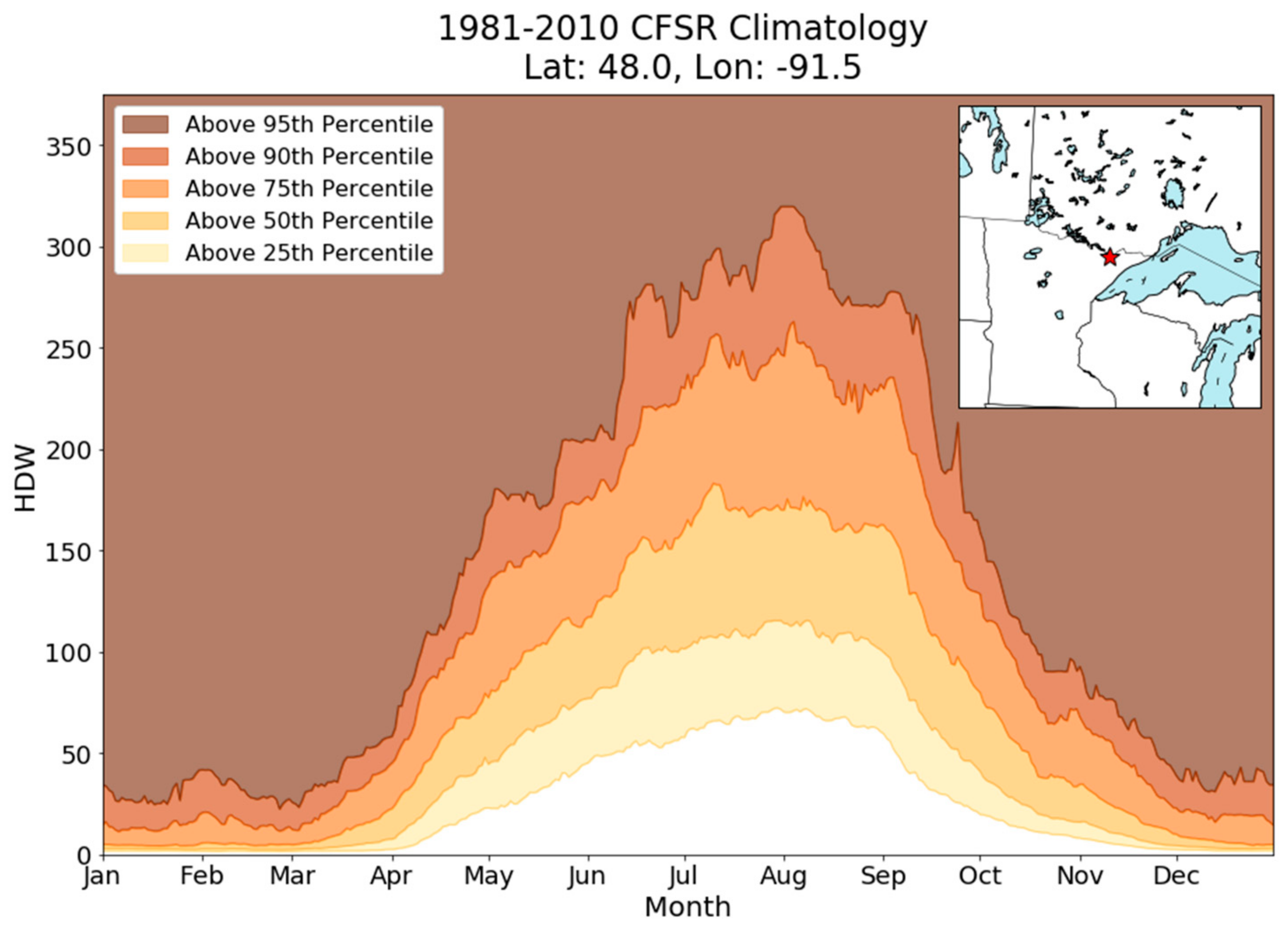
We begin our HDW climatology analysis with a yearly perspective, which shows seasonal variability in HDW for a given location. Figure 1 shows an example plot with the yearly percentiles for the CFSR grid point closest to the Pagami Creek Fire (48.0° N, 91.5° W; see [1,5] for more details regarding this fire). For each day in the climatology, the 25th, 50th, 75th, 90th, and 95th percentiles have been plotted and areas between the percentile bounds have been shaded.
The clearest signal in this analysis is the seasonal cycle. Given this point’s high latitude, we would expect the winter months to experience cold temperatures, so both the saturation vapor pressure and the vapor pressure deficit (VPD) at this location would be small. Thus, even with a strong wind, an HDW value greater than 50 is unlikely in the winter. Comparatively, HDW values in August are routinely much greater due to larger VPDs and a similar likelihood of windy conditions; at this station, the 25th percentile HDW value in August is greater than the 95th percentile value in January. Note that HDW values close to zero can happen at any time of the year due to the effect of precipitation (very low VPD), calm winds, or both. Therefore, HDW will have a much larger range during the warm season in regions with a continental climate that experiences episodic rain events, which substantially lower the VPD compared to days without precipitation.
This result also supports the decision to use 15 days of CFSR data to compute the percentiles for a given day rather than using the entire year. If we had used all 365 days of HDW values over the 30 years to calculate percentiles, many more of the days in August at this location would have been above the 95th percentile and percentiles would be a far less effective discriminator. However, this decision also means that a user must look both at the percentile and the actual HDW value to get a complete picture of the situation. Figure 2 shows the climatological distribution of HDW at 33.0° N, 116.5° W (the location of the 2003 Cedar Fire discussed in [1]), but with every individual HDW value in the climatology also plotted on the chart. Especially noteworthy for this location is the distribution of individual points that are above the 95th percentile line throughout the year. While one would expect some especially high HDW values in the summer, the outlier HDW over 350 in December might also portend a dangerous fire day.
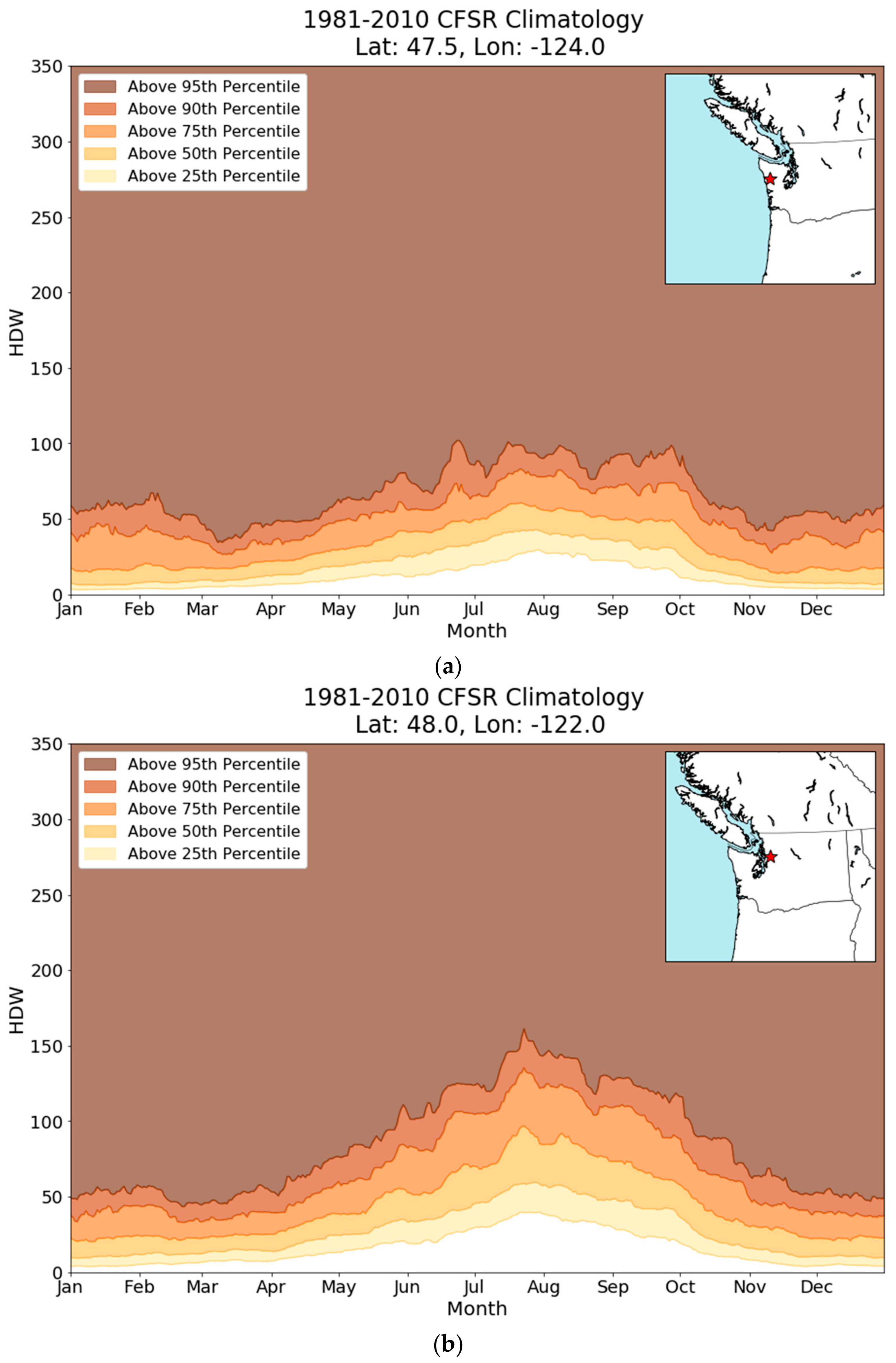
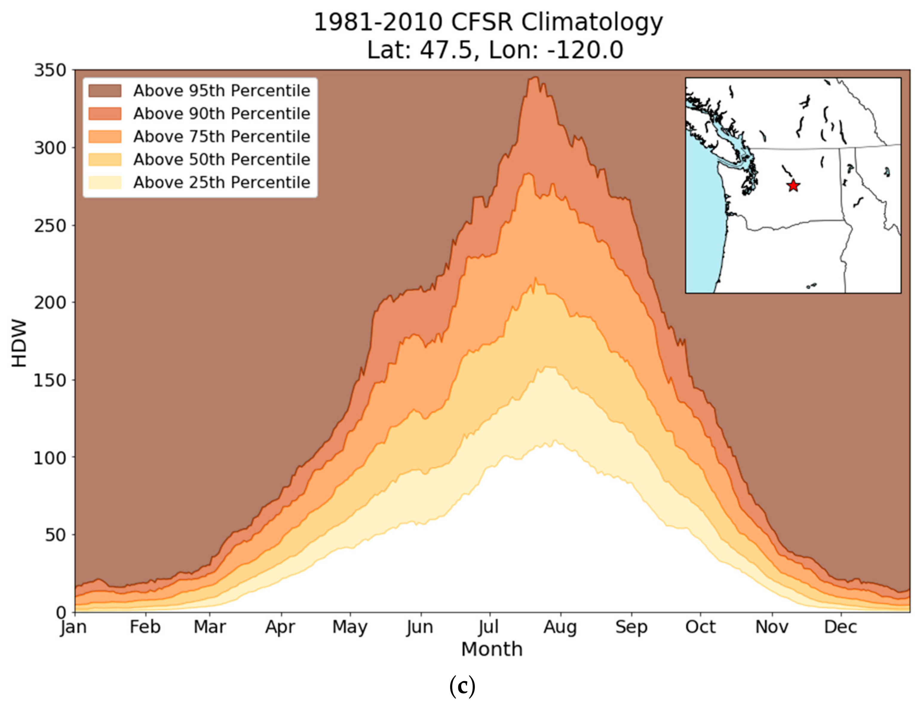
Intercomparison of HDW climatology analyses at nearby points also demonstrates the influence of topographical and climatological variability on HDW. Figure 3 shows a series of three HDW climatology distributions along 47.5° N in Washington State (the point locations are shown in the inset maps). Figure 3a shows the point at 124.0° W, on the windward side of the Olympic Mountains. The climate of that location is dominated by the nearby Pacific Ocean, which causes a relatively small yearly temperature range, small VPDs, and frequent precipitation. The HDW distribution matches this assertion—there is a minor increase in HDW percentile values during the summer months, but the overall distribution is much flatter than seen in northern Minnesota or southern California (cf. Figure 1 and Figure 2).
Figure 3b,c represent the windward (122.0° W) and leeward (120.0° W) sides of the Cascade Mountains, respectively. Both plots show a much more pronounced HDW seasonal cycle than the near-coastal plot, with the plot from central Washington showing the greatest seasonal variation. These results match topographic and climatological expectations; from west to east respectively, the Köppen classifications (e.g., [6]) for these three points are temperate oceanic, temperate Mediterranean, and temperate continental climates. These results also parallel the experience of the wildland fire community. Firefighters know that hot, dry, and windy conditions are more likely to occur east of the spine of the Cascade Mountains in the downsloping region than along the Pacific coast.
With this analysis, note that an HDW value at the 95th percentile does not necessarily imply weather conditions that contribute to dangerous fire behavior. Rather, given the way that the climatology has been defined, a high-percentile value simply suggests anomalous fire-weather conditions for the given time of year. For example, if it is not “fire season” for a given location (like in Minnesota in January), conditions associated with a high-percentile HDW day may not significantly affect any fire that is currently burning. It should also be noted that the choice of the 95th percentile is somewhat arbitrary in these analyses. In a statistical sense, the 95th percentile should be expected to occur 1 day in 20, and it is not necessarily clear in advance whether a 1 in 20 event is enough of an outlier that special attention is warranted. We chose the 95th percentile because this threshold produces an analysis that is straightforward to interpret in multiple locations. However, individual forecasters and fire managers may find that different thresholds would better serve their operational needs.
4. Climatological HDW and Historical Fires
While the climatology alone provides a useful overview of the HDW distribution at a specific location, it is also possible to combine the climatology with a daily trace of HDW values for a given time range to identify the frequency at which these values occur. We demonstrate this capability using the fires from [1], but with the addition of the HDW climatology in the background (using the same contouring and shading conventions presented in the previous section). For each of the cases, we have plotted the 29-day subset of the climatology that matches the 29-day trace of HDW from [1]. Since each of these fires was analyzed in [1], we will focus here on additional insights gained from combining the climatology with the daily HDW trace.
4.1. Pagami Creek Fire (MN, 2011)
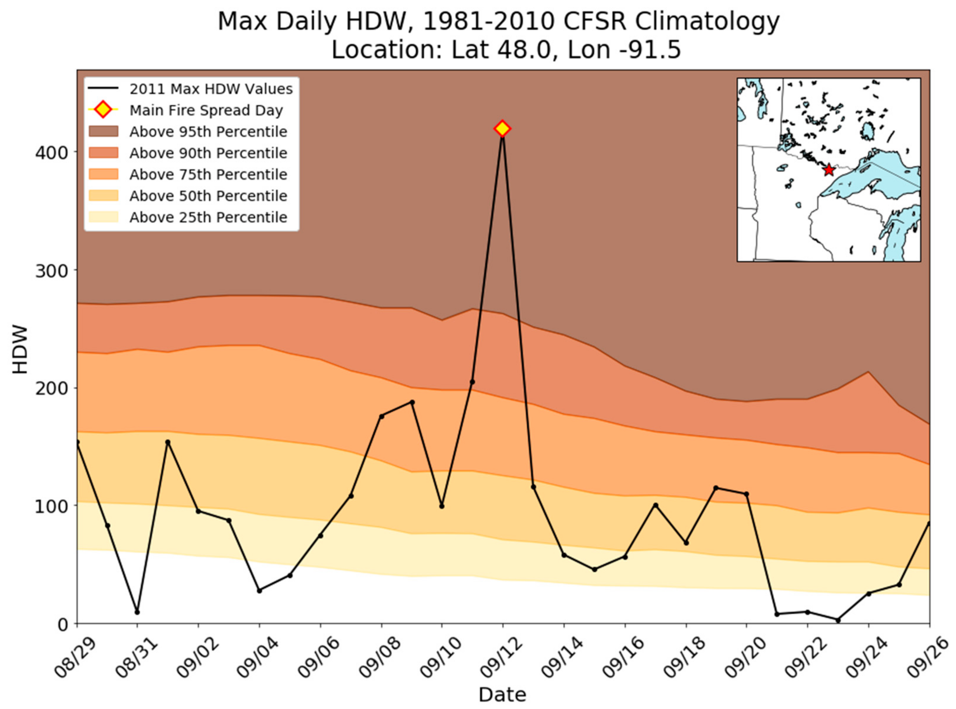
Figure 4 shows the combination of the HDW trace and the climatology for the dates surrounding the large-spread day of the Pagami Creek Fire. As discussed in [1,5], the day with the most “active fire behavior” (12 September) is the highest HDW day compared to the rest of the trace. The additional information from the climatology provides further insights. First, the climatology suggests that Minnesota is well into its autumn transition season, with the HDW values for the climatological percentiles all decreasing over the 29-day period shown. HDW on the largest spread day is well above the 95th percentile, which means that weather conditions were especially anomalous that day. The second-largest spread day was 11 September, when HDW was between the 90th and 95th percentiles. After 13 September, the fire spread much less rapidly, which is consistent with the lower HDW values and lower associated percentiles shown in the figure.
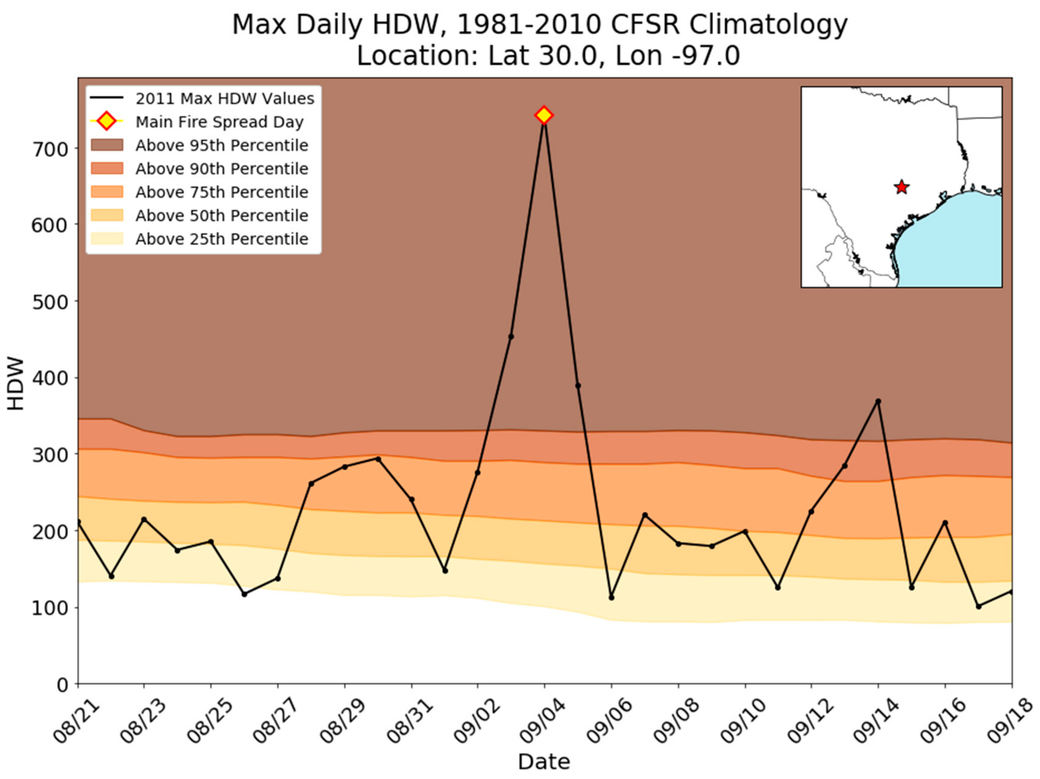
4.2. Bastrop County Complex (TX, 2011)
The series of fires that started on 4 September 2011 near Bastrop, TX, was associated with one of the highest HDW days at that grid point in the entire climatology (Figure 5). Like the Pagami Creek Fire, the most dangerous fire behavior for the Bastrop County Complex coincided with an HDW value well above the 95th percentile, but surrounding days also showed HDW values above the 95th percentile. Unlike the Pagami Creek Fire, only one of the days in the two weeks preceding the fire was below the 25th percentile and many were above the 50th percentile. Central Texas had been experiencing drought conditions for a period of time prior to the fire [7], and we have noted in our analyses that warm-season HDW-climatology values less than the 25th percentile are sometimes associated with thick cloud cover or rain. Thus, when the high-HDW weather conditions occurred on 3 and especially 4 September, the region was primed for dangerous fire behavior.
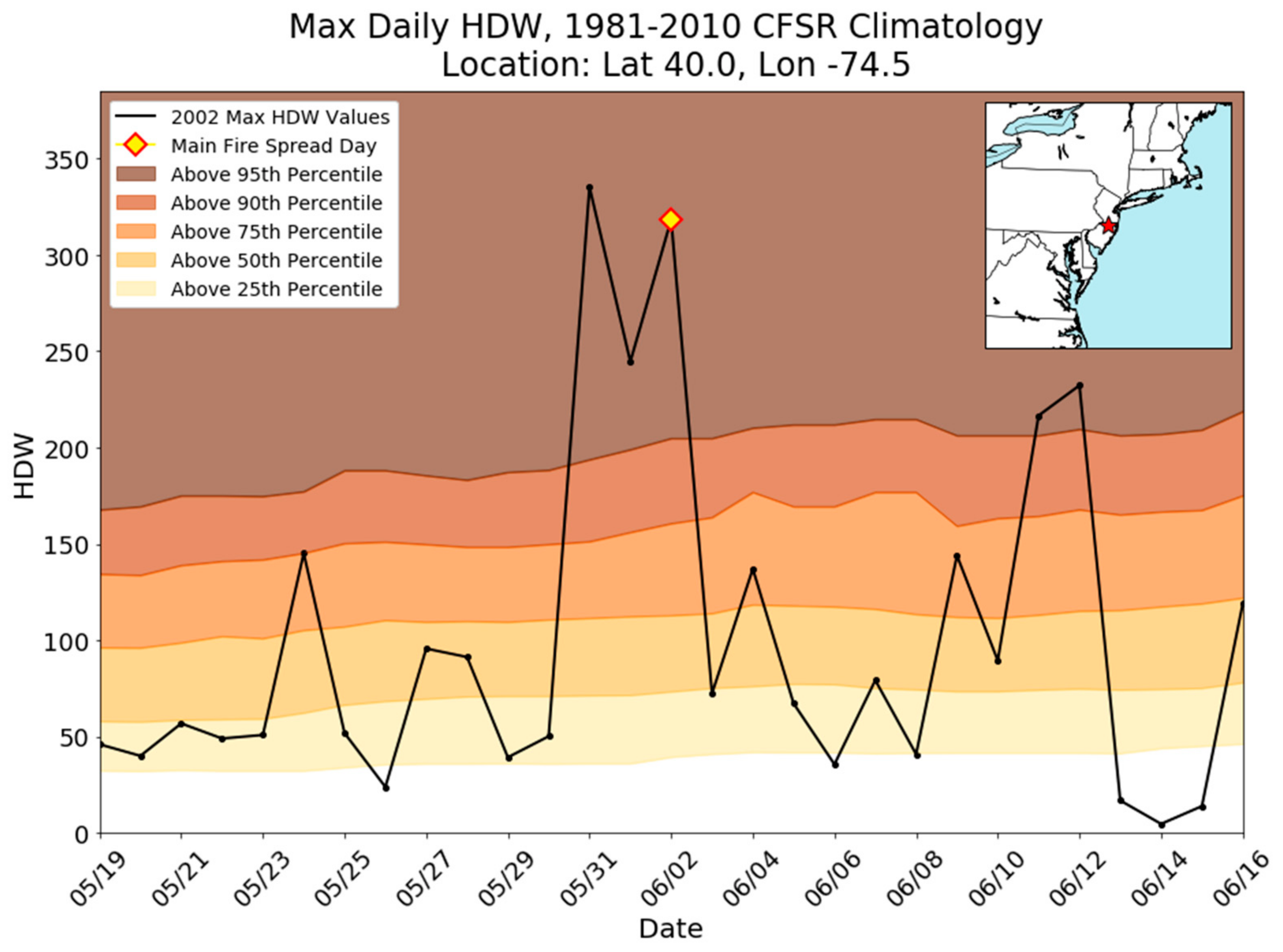
4.3. Double Trouble Fire (NJ, 2002)
The HDW trace and climatology for the Double Trouble Fire are shown in Figure 6. As noted in [1], the Double Trouble Fire HDW trace does not have one clear spike in HDW, but rather three days which were all well above the rest of the examined period. When combining that analysis with the climatology, one can see that 31 May, 1 June, and 2 June were all days with HDW values well above the 95th percentile. While the Double Trouble Fire did not start until 2 June, one can hypothesize that similarly dangerous fire behavior could have occurred on either 31 May or 1 June, especially considering the HDW values that are outliers in the climatology.
This analysis also highlights another very important aspect of both HDW and the HDW climatology—high HDW values can indicate days with conditions that could negatively affect any fires that start on those days, not just fires that already exist. In this sense, accurate forecasts of HDW (with the climatology) may have predictive skill for identifying days when fires could cause significant management difficulties.
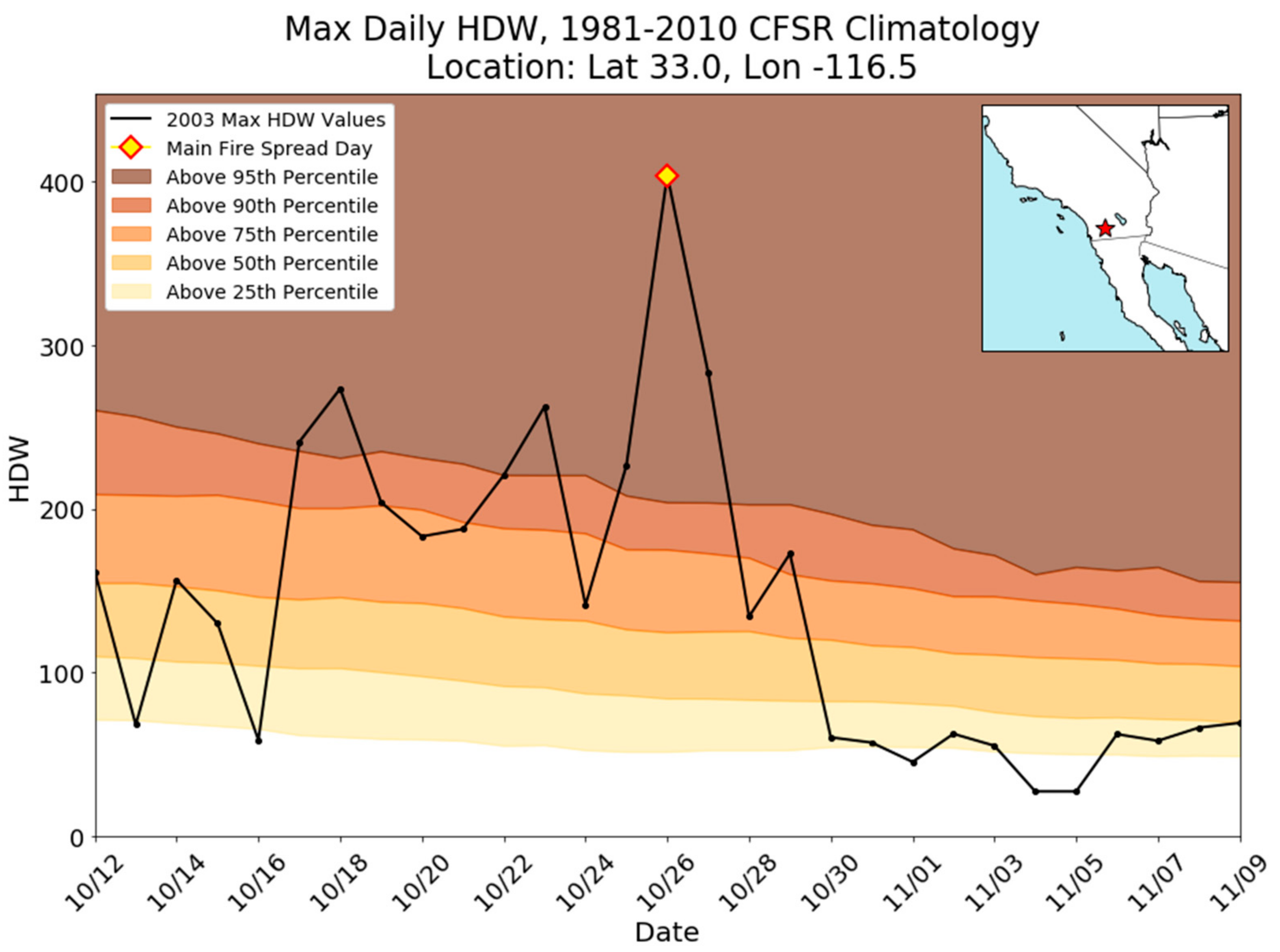
4.4. Cedar Fire (CA, 2003)
The 2003 Cedar Fire in California occurred during drought conditions and was made especially dangerous due to Santa Ana winds on the worst fire day (Figure 7). Preceding the highest-HDW day were nine consecutive days with HDW values above the 75th percentile, four of which were above the 95th percentile. Without the HDW climatology for comparison, it might not be clear to a fire-weather forecaster or a fire manager that the persistent hot-dry-windy weather conditions that had affected southern California were especially anomalous. As in the Bastrop fires, the drought conditions that preceded the Cedar Fire likely contributed to dangerous fire behavior. These results suggest that a multiday record of HDW could be useful when determining the potential for weather conditions to affect a fire. It should be noted that while HDW is formulated to be independent of fuel conditions, the near-surface meteorological variables that are used to calculate HDW (wind speed, temperature, and humidity) are affected by surface conditions. Since HDW uses meteorological inputs from the lowest 500 m of the atmosphere, in most scenarios the effect of vegetation, drought, and other surface features on HDW values will be smaller than on the surface conditions alone.
While daily values of HDW plotted by themselves have value for identifying days on which dangerous fire conditions have occurred, the addition of the climatological percentiles in the background produces a more informative product for users. While this type of analysis has been shown to be useful for historical events (and is necessary to establish that the methodology works), a tool like this also lends itself well to forecasting applications, if appropriate forecast data for comparison with the climatology can be identified.
5. Forecasts of HDW with the HDW Climatology
When looking for appropriate model forecast data to use for HDW, we needed to find a data source that was on the same grid as the HDW climatology and that had the same areal coverage and temporal resolution. We also wanted to find a modeling system that provided ensemble predictions; an ensemble shows forecast spread and thus indicates forecast uncertainty, which helps a fire-weather forecaster determine forecast confidence. The dataset we chose for our analysis is NCEP’s Global Ensemble Forecast System (GEFS; [8]). Like the CFSR, it has a 0.5-degree grid spacing, covers the entire earth, and is updated every 6 h at synoptic times.
HDW is calculated with the GEFS using the same method as with the CFSR (detailed in [1]). However, there are two aspects to the GEFS calculations—the history and the forecasts. For the GEFS history, a 10-day record of the maximum HDW value from the 1200, 1800, and 0000 UTC GEFS control-run analyses is calculated and plotted; this gives the user a sense of the recent HDW conditions for that given point. Then, the forecasts from all 21 GEFS members are processed (the control run and 20 perturbations); for each member, the maximum HDW for the day is plotted. By plotting each member separately, one can determine uncertainty by examining the spread in the forecast values. Since the target audience for this product includes fire-weather forecasters who need data for a morning briefing, we use the 0000 UTC GEFS run for input data (i.e., the graphics are made overnight and are ready for the morning).
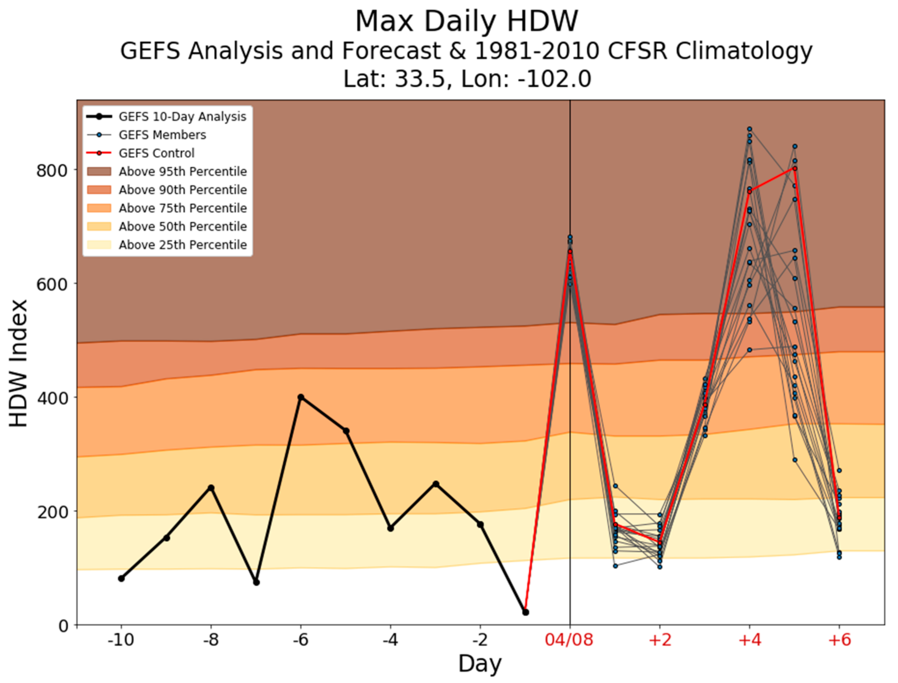
An example forecast plot from 8 April 2018 is shown for a grid point near Lubbock, TX (Figure 8). The recent HDW trace shows large variability, with 2 April (day −6) well above the 75th percentile and 7 April (day −1) showing HDW values below the 25th percentile. The low HDW value on 7 April occurred the day after a strong, fast-moving cold front brought low temperatures and increased cloud cover, resulting in a lower VPD and decreased wind speeds behind the front in Lubbock.
On the forecast side of the plot, the ensembles for day 0 stand out for two reasons: all the GEFS members are predicting values above the 95th percentile and the spread of forecast values is small. This means there is high confidence that anomalous fire-weather conditions will occur (for this time of year), and fire-weather forecasters should be on alert. The two days following 8 April show HDW values mostly below the 50th percentile and the forecast spread is again relatively small, so the potential for weather conditions to make a wildland fire difficult to manage on those days is lower than on the previous day. On days +4 and +5, the GEFS members again forecast anomalously high HDW values, with some members even exceeding an HDW value of 800. However, the ensemble spread for both these days is very large, with a range of roughly 400 on day +5. This suggests that while forecasters should keep an eye on those days, the uncertainty in the forecast is large—information that is useful to fire crews and planners.
A key point here: this HDW forecast product is only as good as the model output that goes into it. If the forecasts from all the GEFS members fail to represent the actual weather patterns that occur on that day, the resulting HDW plots will look normal but will not properly cover the phase space of possible HDW values for the forecast period. Similarly, model forecasts vary from run to run, so the HDW forecast can drastically change as time progresses. Despite these uncertainties, the GEFS forecasts of HDW combined with the CFSR climatology can help identify days that could have increased fire risk due to synoptic- and meso-alpha-scale weather patterns.
6. Discussion and Conclusions
This paper has described and analyzed a climatology of the Hot-Dry-Windy Index (HDW), which was created to provide additional information about individual values of HDW to fire managers and fire-weather forecasters. The climatology was produced using the CFSR and focuses on the contiguous United States, though it will likely be expanded to a global climatology at some point. For practical use, the climatology is described using percentiles because HDW is not a normally distributed quantity and using percentiles is the most straightforward way to identify outliers for non-normal distributions.
The HDW climatology provides insight into near-surface climatic conditions. From the yearly climatology plots (e.g., Figure 3a–c), one can identify temperature and humidity trends that correspond to climate classification systems. Since many fire personnel travel across the country to unfamiliar locations to manage wildland fires, a reference tool like the HDW climatology can quickly orient an individual who is new to the area.
The greatest strength of the HDW climatology is when it is used in parallel with daily traces of observed and/or forecast HDW values. This allows the user to not only follow trends, but to see how those trends compare with historical values. Because HDW is on a continuous scale (as opposed to a binned product like the Haines Index; [9]), both the climatology and the daily trace of HDW can provide useful information about the potential for atmospheric conditions to contribute to dangerous fire behavior for any day, regardless of whether it is an outlier or near the middle of the distribution.
For the four cases examined in [1], the days with the most dangerous fire behavior had HDW values well above the 95th percentile, suggesting that a significant HDW outlier can contribute to dangerous fire conditions on the ground. However, further research is needed to determine if dangerous conditions are unique to extreme outliers. For example, there may be a percentile below which weather conditions prevent all fires from becoming dangerous. This suggests that an investigation into the range of potential fire outcomes at different percentile thresholds is warranted and should be conducted in the future. It should also be noted that fuel conditions can contribute to dangerous fire conditions on days when the HDW value is not an extreme outlier.
Looking forward, this HDW analysis product shows promise as a forecasting tool. By combining the CFSR climatology with a GEFS ensemble history and forecast, we can create a single image that provides seasonal, climatological, and short-term context to help determine the appropriate fire-management response to a given HDW value. While the tool, as presented here, is valuable on its own in its current state, we have identified additional investigations that should be performed to improve its validity. First, while the CFSR and GEFS have the same spatial and temporal characteristics, they are not identical products. Since they are directly compared in the forecast plots, a study that investigates whether there are significant systematic and/or random differences between the two products should be undertaken. Second, the forecasting tool needs to be updated and modified based on how fire-weather forecasters and fire managers use this product operationally.
Author Contributions
A.S. and J.C conceived of this study. J.M. and A.S. produced a first draft of the manuscript, and J.C. participated in editing and refining the manuscript into a final form. J.M. and A.S. completed the numerical analyses and worked with J.C. to produce and finalize the figures. J.C. prepared the manuscript for submission to Atmosphere.
Acknowledgments
This research was partially supported by Research Joint Venture Agreement 12-JV-11242306-067 between the U.S. Forest Service, Northern Research Station, and Michigan State University. The authors thank Brian Potter, Scott Goodrick, Robyn Heffernan, Larry Van Bussum, Sharon Zhong, and a host of National Weather Service Incident Meteorologists for insights provided in discussions during the development of this research.
Conflicts of Interest
The authors declare no conflicts of interest.
References
- Srock, A.; Charney, J.; Potter, B.; Goodrick, S. The Hot-Dry-Windy Index: A new fire weather index. Atmosphere 2018, 9, 279. [Google Scholar]
- Doswell, C.; Schultz, D. On the use of indices and parameters in forecasting severe storms. Electron. J. Sev. Storms Meteorol. 2006, 1, 1–14. [Google Scholar]
- Saha, S.; Moorthi, S.; Pan, H.; Wu, X.; Wang, J.; Nadiga, S.; Tripp, P.; Kistler, R.; Woollen, J.; Behringer, D.; et al. The NCEP Climate Forecast System Reanalysis. Bull. Am. Meteorol. Soc. 2010, 91, 1015–1057. [Google Scholar] [CrossRef]
- Saha, S.; Moorthi, S.; Wu, X.; Wang, J.; Nadiga, S.; Tripp, P.; Behringer, D.; Hou, Y.T.; Chang, H.Y.; Iredell, M.; et al. The NCEP climate forecast system version 2. J. Clim. 2014, 27, 2185–2208. [Google Scholar] [CrossRef]
- Sexton, T.; Menakis, J.; Pence, M. Pagami Creek Fire: Summary of Decisions and Information Used in Making Decisions; Superior National Forest: Duluth, MN, USA, 2012; p. 42. [Google Scholar]
- Kottek, M.; Grieser, J.; Beck, C.; Rudolf, B.; Rubel, F. World map of the Köppen-Geiger climate classification updated. Meteorol. Z. 2006, 15, 259–263. [Google Scholar] [CrossRef]
- Huffman, H.; Saginor, A. Texas tackles devastating fire season with complex, interagency response. Fire Manag. Today 2012, 72, 6–13. [Google Scholar]
- Wei, M.; Toth, Z.; Wobus, R.; Zhu, Y. Initial perturbations based on the ensemble transform (ET) technique in the NCEP global operations forecast system. Tellus A 2008, 60, 62–79. [Google Scholar] [CrossRef]
- Haines, D.A. A lower atmospheric severity index for wildland fire. Nat. Weather Dig. 1988, 13, 23–27. [Google Scholar]
Figure 1.
Centered, 15-day running HDW climatological percentiles per day (shaded) calculated using CFSR data from 1981 to 2010 for the grid point at 48.0° N, 91.5° W. Map inset shows grid point location with a red star.
Figure 1.
Centered, 15-day running HDW climatological percentiles per day (shaded) calculated using CFSR data from 1981 to 2010 for the grid point at 48.0° N, 91.5° W. Map inset shows grid point location with a red star.

Figure 2.
HDW climatological percentiles and inset map as in Figure 1, but for the grid point at 33.0° N, 116.5° W. Black dots represent individual HDW values from the 1981–2010 climatology by day at this grid point.
Figure 2.
HDW climatological percentiles and inset map as in Figure 1, but for the grid point at 33.0° N, 116.5° W. Black dots represent individual HDW values from the 1981–2010 climatology by day at this grid point.

Figure 3.
As in Figure 1, but for grid points at (a) 47.5° N, 124.0° W; (b) 47.5° N, 122.0° W; and (c) 47.5° N, 120.0° W.
Figure 3.
As in Figure 1, but for grid points at (a) 47.5° N, 124.0° W; (b) 47.5° N, 122.0° W; and (c) 47.5° N, 120.0° W.


Figure 4.
HDW climatological percentiles as in Figure 1, but for the 29-day period examined in [1] for the Pagami Creek Fire (centered on 12 September, the largest fire-spread day) at grid point 48.0° N, 91.5° W. The black trace represents HDW values calculated from CFSR for the same 29-day period in 2011.

Figure 5.
As in Figure 4, but for the Bastrop County Complex (grid point 30.0° N, 97.0° W; 29-day period centered on 4 September). The black trace represents HDW values calculated from CFSR for the same 29-day period in 2011.
Figure 5.
As in Figure 4, but for the Bastrop County Complex (grid point 30.0° N, 97.0° W; 29-day period centered on 4 September). The black trace represents HDW values calculated from CFSR for the same 29-day period in 2011.

Figure 6.
As in Figure 4, but for the Double Trouble Fire (grid point 40.0° N, 74.5° W; 29-day period centered on 2 June). The black trace represents HDW values calculated from CFSR for the same 29-day period in 2002.
Figure 6.
As in Figure 4, but for the Double Trouble Fire (grid point 40.0° N, 74.5° W; 29-day period centered on 2 June). The black trace represents HDW values calculated from CFSR for the same 29-day period in 2002.

Figure 7.
As in Figure 4, but for the Cedar Fire (grid point 33.0° N, 116.5° W; 29-day period centered on 26 October). The black trace represents HDW values calculated from CFSR for the same 29-day period in 2003.
Figure 7.
As in Figure 4, but for the Cedar Fire (grid point 33.0° N, 116.5° W; 29-day period centered on 26 October). The black trace represents HDW values calculated from CFSR for the same 29-day period in 2003.

Figure 8.
HDW climatological percentiles as in Figure 1, but for a 17-day period surrounding 8 April at grid point 33.5° N, 102.0° W. The historical trace (7 April and earlier) represents HDW values calculated from GEFS control-run analyses. The forecast traces represent HDW values calculated from each GEFS ensemble member, with the control run plotted in red and perturbation runs in gray.

© 2018 by the authors. Licensee MDPI, Basel, Switzerland. This article is an open access article distributed under the terms and conditions of the Creative Commons Attribution (CC BY) license (http://creativecommons.org/licenses/by/4.0/).
Share and Cite
MDPI and ACS Style
McDonald, J.M.; Srock, A.F.; Charney, J.J. Development and Application of a Hot-Dry-Windy Index (HDW) Climatology. Atmosphere 2018, 9, 285. https://doi.org/10.3390/atmos9070285
AMA Style
McDonald JM, Srock AF, Charney JJ. Development and Application of a Hot-Dry-Windy Index (HDW) Climatology. Atmosphere. 2018; 9(7):285. https://doi.org/10.3390/atmos9070285
Chicago/Turabian StyleMcDonald, Jessica M., Alan F. Srock, and Joseph J. Charney. 2018. "Development and Application of a Hot-Dry-Windy Index (HDW) Climatology" Atmosphere 9, no. 7: 285. https://doi.org/10.3390/atmos9070285
Note that from the first issue of 2016, this journal uses article numbers instead of page numbers. See further details here.