The Effect of Nonlocal Vehicle Restriction Policy on Air Quality in Shanghai


1
Center for Intelligent Transportation Systems and Unmanned Aerial Systems Applications, State Key Laboratory of Ocean Engineering, School of Naval Architecture, Ocean & Civil Engineering, Shanghai Jiao Tong University, Shanghai 200240, China
2
China Institute for Urban Governance, Shanghai Jiao Tong University, Shanghai 200240, China
3
Department of Urban and Regional Planning, University of Florida, Gainesville, FL 32611, USA
*
Author to whom correspondence should be addressed.
Atmosphere 2018, 9(8), 299; https://doi.org/10.3390/atmos9080299
Submission received: 8 June 2018
/
Revised: 24 July 2018
/
Accepted: 28 July 2018
/
Published: 30 July 2018
(This article belongs to the Special Issue Air Quality in China: Past, Present and Future)
Abstract
:In recent years, road space rationing policies have been increasingly applied as a traffic management solution to tackle congestion and traffic emission problems in big cities. Existing studies on the effect of traffic policy on air quality have mainly focused on the odd–even day traffic restriction policy or one-day-per-week restriction policy. There are few studies paying attention to the effect of nonlocal license plate restrictions on air quality in Shanghai. Restrictions toward nonlocal vehicles usually prohibit vehicles with nonlocal license plates from entering certain urban areas or using certain subsets of the road network (e.g., the elevated expressway) during specific time periods on workdays. To investigate the impact of such a policy on the residents’ exposure to pollutants, CO concentration and Air Quality Index (AQI) were compared during January and February in 2015, 2016 and 2017. Regression discontinuity (RD) was used to test the validity of nonlocal vehicle restriction on mitigating environmental pollution. Several conclusions can be made: (1) CO concentration was higher on ground-level roads on the restriction days than those in the nonrestriction days; (2) the extension of the restriction period exposed the commuters to high pollution for a longer time on the ground, which will do harm to them; and (3) the nonlocal vehicle restriction policy did play a role in improving the air quality in Shanghai when extending the evening rush period. Additionally, some suggestions are mentioned in order to improve air quality and passenger health and safety.
1. Introduction
With the rapid development and urbanization process in China, the transportation structure has been greatly changed and people rely more and more on motor vehicles instead of any other travel mode. Total car ownership is increasing with the situation now where China has become the world’s leading market of new automobiles [1,2]. At the same time, the expanded growth of motorization has contributed to a series of problems such as air pollution, oil price hikes, congestion, and growing greenhouse gas emissions [3]. For example, rapid motorization in Beijing has resulted in serious congestion and the average network travel speed decreasing by 3.2% and 4.9%, respectively, within the 5th Ring Road during 2010 in AM and PM peak hour [4]. According to the United States Environmental Protection Agency, motor vehicles are an important source of air pollutants including carbon monoxide (CO), oxides of nitrogen (NOx), sulfur dioxide (SO2), volatile organic compounds (VOC), and particulate matter (PM) [5,6,7].
Large-scale urban smog and haze phenomena, which are partly caused by vehicular emissions, have raised a wide range of concerns because increasing air pollution has been found to be associated with adverse human effects [8] with many epidemiological studies proving this fact [9,10,11,12,13]. Compared to inhalable particles (PM10), PM2.5 have more serious effects on human physical health because their small size can carry a variety of other pollutants, which means that the smaller the particle size, the greater the risk it would bring to the human body [14]. Furthermore, recent studies of epidemiology and toxicology showed that long-term exposure to high concentrations of CO or NOx also had a negative effect on human health. NOx may aggravate respiratory infections and symptoms (sore throat, cough, nasal congestion and fever), and increase the risk of chest cold, bronchitis and pneumonia in children [15]. Regarding CO, one study found that even several hours of exposure to air containing 0.001% of CO can lead to death [16] as this gas prevents the uptake of oxygen by the blood so that it can lead to a significant reduction in the supply of oxygen to the heart, particularly in people suffering from heart disease [15]. In addition, CO produced in heavy traffic can cause headaches, drowsiness and blurred vision.
In order to alleviate the traffic pressure or take control of the pollutants emitted by motor vehicles, some traffic restrictions have been applied as a quick method. The vehicle restriction policy mainly refers to those measures that restrict the access or travel of certain types of vehicles in urban areas. Such measures can often reduce the number of motor vehicles in restricted areas and mitigate traffic congestion in the short term. However, previous studies have debated whether the vehicle restriction policy can improve urban air quality. For one thing, there have been some studies holding positive views about the effect of traffic restriction policies on air quality. For instance, Hochstetler et al. established an estimation model to evaluate the license restriction policy implemented in São Paulo, Brazil, since 1997, and found the license restriction policy successfully reduced the CO emissions of urban motor vehicles by 19% [17]. Troncoso et al. established a linear regression model to analyze the impact of vehicle restriction policy in Santiago on air quality based on the control of temperature, pressure, precipitation and other meteorological conditions. Their results showed that after the traffic restriction, pollutants such as CO, NOx, PM10 and PM2.5 in the urban atmosphere had decreased at different degrees except SO2 [18]. However, on the other hand, some negative views have also been found. Davis et al. found that air quality did not significantly improve by analyzing the restriction policy (Hoy No Circula, HNC) in Mexico City based on the control of wind speed, temperature and other factors by using the Regression Discontinuity (RD) design. They speculated that the policy has stimulated individuals to purchase additional vehicles [19]. Onursal et al. also believed that the effect of HNC control policy on the promotion of air quality in Mexico City was limited [20]. Interestingly, Salas et al. believed that changes in the use of different time windows to estimate the effect of the HNC and changes in the length of the time trend polynomial (which controls for time-varying factors) revealed dramatic changes in the conclusions obtained from the approach used by Davis (2008). Furthermore, he concluded that air pollution was reduced by 5% to 18% in the first month after carrying out the traffic restriction policy by reanalyzing the case of Mexico City. However, the concentration gradually increased and the policy became weaker in reducing the air pollution [21].
The domestic vehicle restriction administration has been implemented since the 2008 Beijing Olympic Games and has also accumulated some relevant research. However, these studies do not present the same results regarding the restriction policy in Beijing either. For one thing, Cai et al. analyzed the concentration of pollutants in different periods in one day based on the odd–even day vehicle prohibition policy considering the association with location factors and wind factors during the 2008 Beijing Olympic Games. The results showed that the restriction policy reduced the concentration of CO, PM10, NO2 and O3 more than 30% [22]. Viard et al. found that the air pollutant concentration decreased by 19% and 8% during the day based on air quality daily data considering the Beijing odd–even restriction policy and the one-day-a-week restriction policy, respectively [23]. Nevertheless, some experts have concluded that the vehicle restriction policy in Beijing had no effect on air quality improvement [24]. Liu et al. concluded that if the public traffic system did not improve synchronously, commuters would not change travel mode choice so the reduction of air pollution was quite limited based on the perspective of the theory of planned behavior, the implementation of questionnaires, and structural equation modeling of different assumptions [25]. Moreover, Zhao et al. collected the data of the concentration and distribution of PM at the 2012 Lanzhou International Marathon during the restriction policy. He found that the concentration of all kinds of particles decreased in different degrees. A 0.5–1 µm particle concentration was closely related to the number of non-CNG (compressed natural gas)-powered vehicles, indicating that the use of reasonable environmental technology also had a greater impact on the quality of the air [26].
To sum up, there is still some controversy over whether the positive effects of the policy on air quality exist. However, these studies did not consider nonlocal vehicle restrictions and this is also an essential component of air pollution control policy that can no longer be ignored. Unfortunately, our literature review found little research on this policy. While the benefit of traffic management lasting for tens of days or several months is generally appreciated, until now, the impact of local short-period (several hours) traffic restriction on urban air quality is largely unknown, despite its potential as a mitigation measure for air pollution, especially for alleviating air pollution under adverse meteorological conditions. As such, there is still a major research gap to be filled. Therefore, in our study, we investigated whether nonlocal vehicle restrictions have improved air quality in Shanghai.
2. Materials and Methods
2.1. Policy Introduction
Shanghai is the chief metropolis and also the commercial and financial center of China. It is bounded by longitude 120°52′–122°12′ E and latitude 30°40′–31°53′ N, and is located on the eastern edge of the Yangtze River Delta, with a total area of 6340 km2 and population of 24 million as of 2016. During the past two decades, Shanghai has witnessed a population explosion, economic prosperity, and rapid urbanization [27]. For instance, the disposable income per capita of Shanghai was 7333 USD with a gross domestic product of 366 billion USD, whereas the income per capita of urban residents was 7788 USD and the income per capita of rural residents was 3412 USD in 2015 [28]. Furthermore, in recent years, urbanization and economic development have led to rapid increases in vehicle ownership and usage in Shanghai; according to the Shanghai Statistics Bureau, the number of registered vehicles almost doubled from 2006 to 2017, increased at an average annual rate of 8.7%, reaching 4.7 million [29]. The rapid growth in motor vehicle ownership has provided convenience to people’s lives, but it has also brought externalities at the same time such as traffic jams, air pollution, energy consumption, and the shortage of land resources. According to the Alibaba Cloud and Gaode Map, Shanghai is one of the ten most congested cities in China. More importantly, in the field of transportation environment, more and more studies have found that particulate matter is one of the pollutants that is majorly contributed by road traffic, and it has been estimated that 90% of urban air pollution in fast-growing cities in developing countries can be attributable to motor vehicle emissions [30]. In a bid to alleviate road traffic congestion and balance traffic volume on the elevated and ground-level roads, Shanghai began to implement the nonlocal vehicle restriction policy in 2002.
Road space rationing policies have emerged as regulatory measures to mitigate the vehicle emission and traffic jam problems in recent years. Some cities in China have adopted the traffic-induced method, traffic restriction methods, and other control means to improve the traffic conditions. For example, Beijing has been implementing even–odd license plate and one-day-per-week policies since 2008. In addition, the Yellow-label car restriction policy was imposed in Beijing to prohibit those vehicles that could not meet the emission standards from entering the city. Additionally, these policies also intended to realize the goal of emissions reduction of the whole road network. For Shanghai, there has been a portfolio of policies to manage vehicle ownership and travel. Like Singapore, Shanghai has been imposing a license auction system since 1992. In addition, vehicles registered under suburban plates were prohibited from entering areas within the outer ring road. Moreover, vehicles with nonlocal license plates have not been allowed to enter the elevated expressways within the outer ring road of Shanghai since 2002. This policy has mainly focused on vehicles with nonlocal license plates, which have been prohibited in some road segments during the designated period for one day (except the weekends and legal holidays). The detailed information is shown in Table 1.
However, there were some changes made to the nonlocal vehicle restriction policy in different years in Shanghai and these changes mainly focused on the prohibition period and prohibited roads. From 16 December 2002 to 15 April 2015 (except for weekends and legal holidays), motor vehicles with nonlocal license plates were prohibited from entering the elevated roads such as the Yan’an Elevated Road, Inner Ring Elevated road, North–South Elevated Road, Yixian Elevated Road, Humin Elevated Road, Lupu Bridge, Middle Ring Road, and Huaxia Elevated Road during the rush hour (7:30–9:30 and 16:30–18:30). Moreover, the prohibition period was extended (7:00–10:00 and 16:00–19:00) from 15 April 2015 to 15 April 2016 (except for weekends and legal holidays) and the prohibited roads stayed the same. The restriction policy changed further in 2016. Not only were more roads added onto the restriction list for nonlocal vehicles, but the restriction time period was also extended. From 15 April 2016 (except for weekends and legal holidays), the prohibition time during rush hour in the evening was extended again (7:00–10:00 and 15:00–20:00). Furthermore, Luoshan Road, Shenjiang Elevated Road, Nanpu Bridge and the Yan’an Road Tunnel were added onto the list of restricted roads. While the main purpose of restriction policies is to manage traffic, it is equally important to investigate the impact of this policy on air quality, which is the focus of this research.
2.2. Data Description
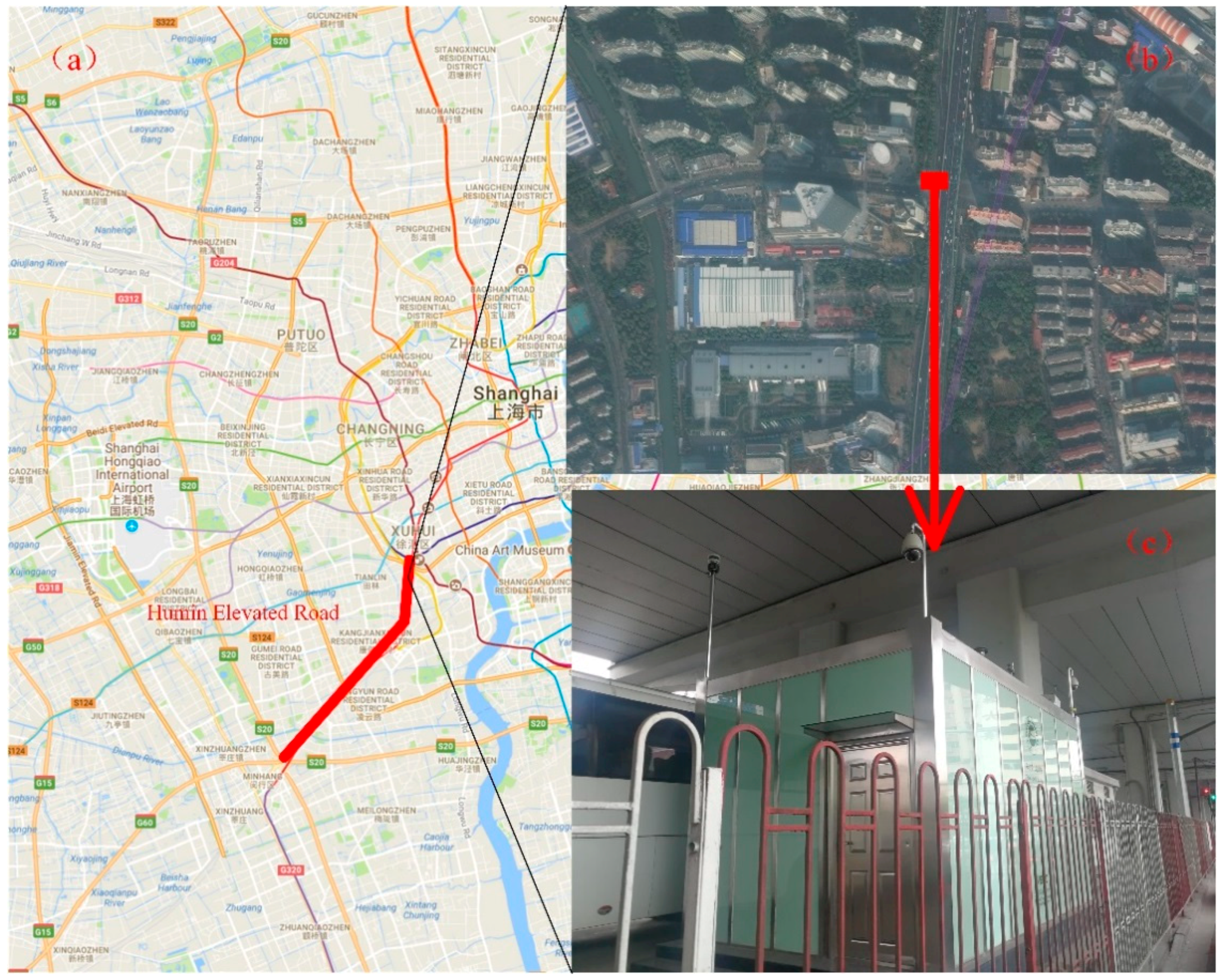
The data were provided by Shanghai Environmental Monitoring Center (SEMC) and included the concentration of five kinds of pollutants, NO2, CO, NOx, NO and PM2.5, from 1 January 2015 to 28 February 2017 at the air pollution monitoring station. The air pollution monitoring station is Xuhui Station and is located just under the Humin Elevated (8 m high) Road near the Caoxi Road subway station (Figure 1). Furthermore, the Xuhui monitoring station was chosen as the Humin Elevated Road has the function of connecting Shanghai’s urban and suburban areas as well as the neighboring province of Zhejiang, so there are many cars with nonlocal license plates running on these corridors. For example, when car owners in Minhang district want to go to a downtown area such as Xujiahui, the Humin Elevated Highway is the best option. Due to the nonlocal license plate restriction policy, those drivers can choose to use the elevated road at nonrestricted hours or the ground-level road at restricted hours to get to their destination. In addition to the emissions from traffic, there are no other major pollutant sources nearby. The selected experimental areas were surrounded by many residential areas. Therefore, the Xuhui air pollution monitoring station was a good choice to study the effect of the restriction policy on human exposure to pollutants. The resolution of data that we obtained was one hour and the number of data records was 18,530 (missing rate: 2.35%). At the same time, we obtained the historical data of AQI from the internet (http://tianqi.2345.com/). AQI is a comprehensive evaluation metric for air pollution, which is computed based on the concentrations of six regulatory air pollutants including PM2.5, PM10, SO2, NO2, O3 and CO.
In this study, we mainly used AQI and CO concentrations for analysis. Other air pollutants such as NO2 and NO are very reactive and they are usually not considered as the trace gases of traffic emissions. However, CO is much more stable and is usually considered as the trace gas of traffic emissions [31].
2.3. Method
In the existing studies, three methods have been applied to test the effect of the restriction policy on air quality: (1) single-difference method: this method is just simply comparing the change of air quality before and after the restriction period; (2) benchmark: this method compares air quality with other cities (control group); and (3) regression discontinuity: whether there is a sudden change in air quality at the policy implementation point or not.
To sum up, the single-difference method is rather rough to test the effect of restriction policy, not only because we cannot distinguish the effect of restriction policy and other policies in Shanghai, but it also cannot differentiate the inherent tendency of air quality; benchmark, however, can partially overcome the inherent trend of air quality itself. Furthermore, it is very hard to find a twin city similar to Shanghai without a nonlocal vehicle restriction policy. Furthermore, benchmark cannot also distinguish the effect of restriction policy and other policies in Shanghai. RD was first introduced by Campbell and began to be widely applied to economic research in the late 1990s [32]. RD is one of the most trustworthy methods in the quasi-experimental method, which is similar to random experiment. The great advantage of RD is that it can overcome the endogenous problem of parameter estimation so that it can reflect the causal relationship between the variables accurately. At the same time, as the key hypothesis of the RD method can be verified by statistical analysis, the estimation results of RD are easy to test.
RD can identify well the effect of the restriction policy. The basic content of RD is that if the policy can be regarded as a sudden change factor (like restriction policy), some methods can be adopted to differentiate this policy from other factors that are continuous variables. In detail, if a sudden change of air quality before and after the implementation of the policy can be observed while other factors can be identified as continuous change, we do have reason to believe that the sudden change of air quality is caused by the restriction policy. If not, the policy can be seen as invalid.
Considering only one break point of policy, according to Angrist and Pischke [33], the estimation equation in the break point is as follows:
where is the observed air quality in the day t; is the dummy variable which represents the restriction policy implementation; is the error term; is the time difference between and ; and means the polynomial function of variable .
3. Results and Discussions
3.1. Comparison of CO Concentration
Due to the limitation of the time span of the data, which is between 1 January 2015 to 28 February 2017, to explore the effect of nonlocal vehicle restriction policy on pollutant concentration and human exposure, unnecessary factors should be removed such as the change of temperature and relative humidity due to seasonal variation. Therefore, we used the data from January and February of 2015, 2016 and 2017, which belonged to the same period to avoid seasonal variation. In addition, the data during January and February in 2015, 2016 and 2017 belonged to the three different policy periods, respectively, so this arrangement was rather suitable. In order to distinguish these three different restriction policies between 2015 and 2017, we called the policy in January and February, 2015 as Policy 1, the policy in January and February, 2016 as Policy 2, and the policy in January and February, 2017 as Policy 3. Specific information can be referred to in Table 1.
3.1.1. Comparison of Pollutant Concentration in Restriction Days and Nonrestriction Days
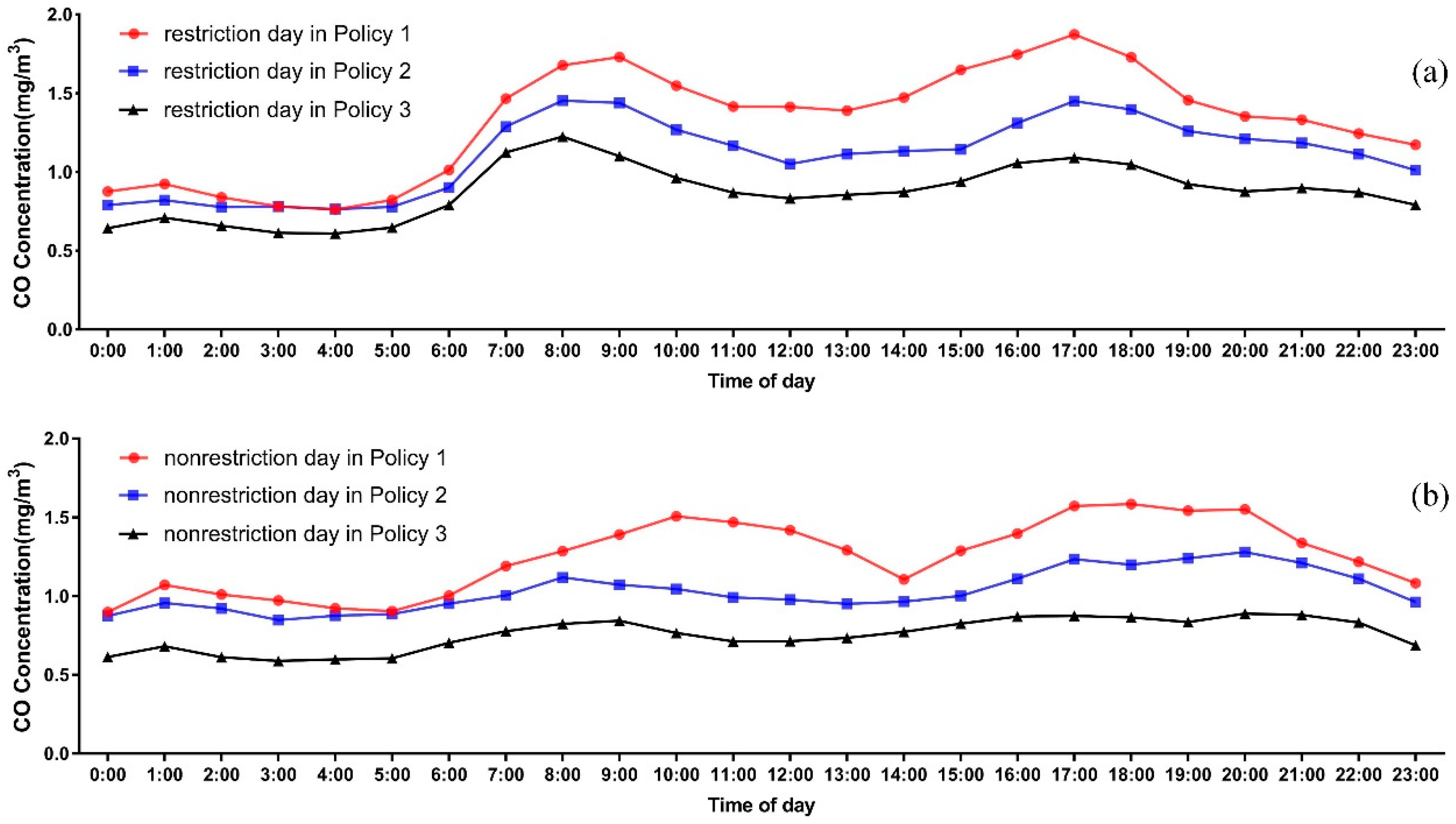
We evaluated the CO concentration in each hour on the restriction days and nonrestriction days as CO is more stable and the cycle of generation and elimination is longer compared to PM2.5 and NOx. At first, we used the number of restriction days (37 days in Policy 1, 38 days in Policy 2, and 38 days in Policy 3) and nonrestriction days (22 days in Policy 1, 22 days in Policy 2, and 21 days in Policy 3) to calculate the average CO concentration in each hour as the distribution of pollutants in a typical restriction day and a typical nonrestriction day.
The results of the detailed information of CO are shown in Figure 2. In terms of the results, several findings were as follows: For one thing, CO concentration apparently changed along with the time and diurnal phenomena of traffic flow; for another, CO concentration was generally higher on the restricted days than that on the nonrestriction days in the ground-level road—for CO, the maximum concentrations in the restriction period were 30.5% higher in 2015, 34.2% higher in 2016, and 48.6% higher in 2017 than those in the nonrestriction period.
3.1.2. Comparison of CO Concentration in Different Policy Situations
In this section, the CO concentrations before and after the implementation of different policies were compared. The results are as shown in Figure 3. Furthermore, the number of restriction days and nonrestriction days were used to calculate the average concentration of three different pollutants in each hour as the distribution of pollutants in a typical restriction day and a typical nonrestriction day in 2015, 2016 and 2017.
The results indicated that CO concentration in each hour showed a decreasing trend along with time. The highest CO concentration in each hour existed in 2015 and the lowest CO concentration in each hour existed in 2017 whether it was a restriction day or not. In detail, on restriction days, the concentration of CO in the restriction period in 2017 was 43% lower than that in 2015 and 27.8% lower than that in 2016; for another, on nonrestriction days, the concentration of CO in the restriction period in 2017 was 51.5% lower than that in 2015 and 33.5% lower than that in 2016.
3.2. Comparison of AQI
The detailed information of the comparison is as follows (Table 2). From Table 2, the following findings can be summarized: For one thing, regardless of whether it was a restriction day or nonrestriction day, from 2015 to 2017, the average AQI decreased, which meant that the air quality improved; for another, the average AQI was generally lower on the restriction days than on the nonrestriction days, but the difference was rather small. For example, the AQI was 6% higher on nonrestriction days in 2015, 5% higher on nonrestriction days in 2016, and 3% lower than on restriction days.
3.3. Regression Discontinuity Analysis
Even though the air quality was better after implementing the different restriction policies, it was still hard to tell the effect of the restriction policy on improving the air quality. Therefore, the RD method was used to better understand the significance of the restriction policy for air quality in a quantified way. The basic idea of the study was as follows: Assume that before the implementation of the restriction policy, the air quality in Shanghai changed smoothly with time without the effect of other exogenous factors such as political and economic factors. If air quality in Shanghai had break points before and after carrying out the new restriction policy, we can conclude that the change of air quality was caused by the restriction policy.
The object of RD usually includes two parts: the sample affected by the policy and the sample that is not affected by the policy. The basic idea of RD is to delimit a critical value at first. Then, the interval samples, which were approximated to random distribution around the critical value, were analyzed by regression model to observe the significant changes in the target variables. There are more and more empirical studies using the regression discontinuity design method since the 1990s. This method is mainly used in the analysis of causality and policy evaluation such as in the fields of labor and education economics, political economics, environmental economics and development economics; for example, Hahn et al. have undertaken the theoretical deduction of the RD model and put forward a corresponding estimation method [34].
3.3.1. Regression Discontinuity of CO Concentration on a Typical Restriction Day
According to the previous conclusion in Section 3.1, we found that CO concentration may have break points during the restriction period on the ground-level road. Therefore, we analyzed the restriction period to see if there was any potential break point on the restriction days and nonrestriction days. As the restriction policy did not belong to the integral time during Policy 1, we mainly focused on Policies 2 and 3. These two restriction policies were the same in the morning, but Policy 3 was extended by 2 h when compared to Policy 2 in the evening rush period.
At first, we selected four time points, which were the start or end points of the restriction period for analysis, namely: 3:00 p.m., 4:00 p.m., 7:00 p.m., and 8:00 p.m. When the restriction policy was proposed, not all drivers were involved immediately. Conversely, this process occurred progressively instead of the complete change of influence that coincided with RD. Therefore, the RD method was used in this study where the restriction was the drive variable and year was the tool variable. Next, we set the data before and after the restriction period as the control group and experimental group, respectively. Finally, the method of parameter estimation was used to examine the influence of restriction policy on air quality. The equation of the RD method is as follows,
where is the concentration of pollutant in time i; is the dummy variable which is equal to 0 when time i is out of the restriction period and is equal to 1 when time i is in the restriction period; BD represents the time difference between time i and the critical value; means the polynomial function of variable BD; and is the error term.
Through the Stata software, the results of the RD of CO concentration could be obtained at different times (Table 3). During Policy 2, the results showed that after entering the restriction period, the CO concentration will increase by 0.159mg/m3 with the significant influence at the p < 0.001 level; after exiting the restriction period, the concentration of CO will be reduced by 0.85mg/m3 with the significant influence at the p < 0.001 level. During Policy 3, the results showed that after entering the restriction period, the CO concentration will increase by 0.056 mg/m3 with the significant influence at the p < 0.01 level; and after exiting restriction period, the CO concentration will be reduced by 0.069 mg/m3 with the significant influence at the p < 0.01 level.
In detail, when the restriction period starts, the concentration of CO will increase and when the restriction period ends, the CO concentration will decrease. To sum up, when the restriction policy extends the restriction period, it will cause a longer period of high concentration of CO. The detailed information of the RD results is shown in Figure 4.
3.3.2. Regression Discontinuity of AQI
Furthermore, when the restriction policy was proposed, not all drivers were involved immediately. Conversely, this process happened progressively instead of a complete change of influence which coincided with the RD. Therefore, the RD method was used in this study where the restriction was the drive variable and year was the tool variable. Next, we set the data before and after the restriction policy as the control and experimental groups, respectively. Finally, the method of parameter estimation was used to examine the influence of restriction policy on air quality. The equation of the RD method is as follows,
where is the AQI on day i; is the dummy variable which is equal to 0 when day i is before Policy 2 or Policy 3 and is equal to 1 when day i is after Policy 2 or Policy 3; BD represents the day difference between day i and the critical value; f(BD) means the polynomial function of variable BD; and is the error term.
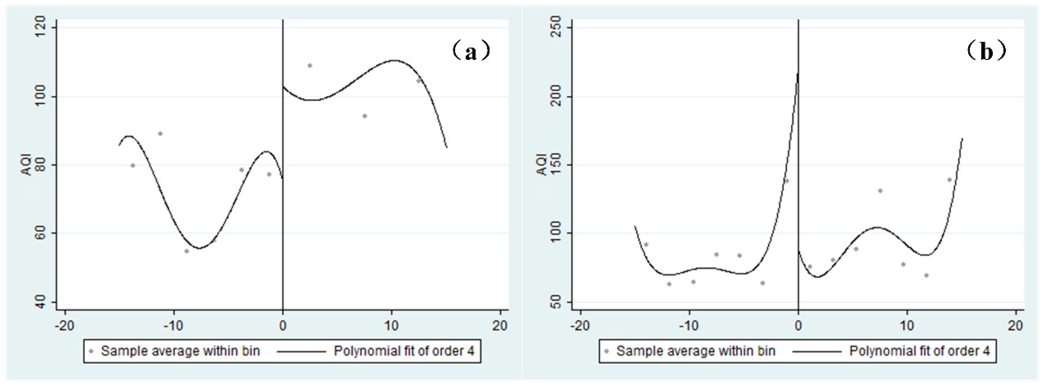
We respectively selected the 15 days before and after the implementation of Policy 2 and Policy 3. Through Stata software, the results of RD of AQI were obtained at different times. From Table 4, during Policy 2, the results showed that AQI will increase by 13 with no significant influence; during Policy 3, the results show that AQI will decrease by 88 with the significant influence at p < 0.001 level.
From Figure 5, we can conclude that after the implementation of Policy 2, the AQI in Shanghai still maintained an increasing trend; in contrast, the AQI decreased sharply after 15 April 2016 (Policy 3). Even though the extended time was the same (two hours) in Policies 2 and 3, the distribution was different. Policy 3 was mainly extended for two hours during the evening rush hour when more vehicles were involved when compared to Policy 2. It is reasonable as to why these two restriction policies caused different results.
3.3.3. The Validity and Stability Test of RD
For one thing, the validity of the regression discontinuity results mainly depends on the fact that the drive variable itself is not artificially manipulated. Considering that the tool variable in this paper was the time variable, at the same time, the time variable was not manipulated artificially. Furthermore, the drive variable was the change of “restriction policy”. Since the restriction policy changed, it only existed when the drivers were involved. Additionally, other variables were continuous. To sum up, the hypothesis met the standard where the driving variable was not affected by human manipulation.
For another, in this paper, based on the original sample data, we added the weather sample data such as maximum temperature and minimum temperature to reconstruct the RD equation. The results are shown in Table 5.
Compared with Table 4 and Table 5, it was found that the coefficients of dummy variables varied at different degrees after the expansion of the sample data, but the change amplitude was not significant. Furthermore, the positive and negative properties, and the significance of the dummy variables, did not change. To sum up, it was considered that the RD model constructed in this paper was stable.
4. Conclusions
In this article, the effect of nonlocal restriction policy on air quality in Shanghai was investigated and tested. In conclusion, the present study suggests that the different nonlocal vehicle restriction policies had different consequences for improving the air quality. Furthermore, CO concentration was higher on the ground-level road on the restriction days than on the nonrestriction days, and the extending of the restriction period will increase the concentration of pollution on the ground, which will cause harm to commuters. Therefore, it is important to understand the effectiveness of the restriction policy, and future studies focused on the long-term health effects of restrictions are also necessary for policymakers. Additionally, some suggestions have been mentioned to improve air quality and passengers’ health and safety on ground roads; for example, a protective belt could be built and vegetation on both sides of the road added.
In follow-up studies, we expect to consider more variables to construct an evaluation system of the nonlocal vehicle restriction policy. Furthermore, field experiments and a vehicle emission model will be supplemented to calculate the emission inventory in Shanghai.
Author Contributions
J.L. wrote the main manuscript text and analyzed the data. Z.-R.P. provided the original research ideas and framework. Z.-R.P., B.L. and X.-B.L. edited this manuscript. J.L. and X.B.L. produced and finalized the figures. Z.-R.P. is the PI of the respective grant that provided funding and supervised the study and has carefully edited the paper. All authors reviewed the manuscript.
Funding
This research was funded by the National Social Science Foundation of China with grant number 16ZDA048.
Conflicts of Interest
The authors declare no conflict of interest.
References
- Dargay, J.; Gately, D.; Sommer, M. Vehicle Ownership and Income Growth, Worldwide: 1960–2030. Energy J. 2007, 28, 143–170. [Google Scholar] [CrossRef]
- Haddock, R.; Jullens, J. The Best Years of the Auto Industry Are still to Come; Booz & Company: New York, NY, USA, 2009. [Google Scholar]
- Sun, C.; Zheng, S.; Wang, R. Restricting driving for better traffic and clearer skies: Did it work in Beijing? Transp. Policy 2014, 32, 34–41. [Google Scholar] [CrossRef]
- Li, P.; Jones, S. Vehicle restrictions and CO2 emissions in Beijing—A simple projection using available data. Transp. Res. Part D Transp. Environ. 2015, 41, 467–476. [Google Scholar] [CrossRef]
- Brook, J.; Poirot, R.; Dann, T.; Lee, P.H.; Lillyman, C.; Ip, T. Assessing Sources of PM2.5 in Cities Influenced by Regional Transport. J. Toxicol. Environ. Health 2007, 70, 191–199. [Google Scholar] [CrossRef] [PubMed]
- Masri, S.; Kang, C.M.; Koutrakis, P. Composition and sources of fine and coarse particles collected during 2002–2010 in Boston, MA. J. Air Waste Manag. Assoc. 2015, 65, 287–297. [Google Scholar] [CrossRef] [PubMed] [Green Version]
- Kavouras, I.G.; Koutrakis, P.; Cereceda-Balic, F.; Oyola, P. Source apportionment of PM10 and PM2.5 in five Chilean cities using factor analysis. J. Air Waste Manag. Assoc. 2001, 51, 451–464. [Google Scholar] [CrossRef] [PubMed]
- Cohen, A.J.; Brauer, M.; Burnett, R.; Anderson, H.R.; Frostad, J.; Estep, K.; Balakrishnan, K.; Brunekreef, B.; Dandona, L.; Dandona, R. Estimates and 25-year trends of the global burden of disease attributable to ambient air pollution: An analysis of data from the Global Burden of Diseases Study 2015. Lancet 2017, 389, 1907–1918. [Google Scholar] [CrossRef]
- Hoek, G.; Brunekreef, B.; Goldbohm, S.; Fischer, P.; van den Brandt, P.A. Association between mortality and indicators of traffic-related air pollution in the Netherlands: A cohort study. Lancet 2002, 360, 1203–1209. [Google Scholar] [CrossRef]
- De Kok, T.M.C.M.; Driece, H.A.L.; Hogervorst, J.G.F.; Briede, J.J. Toxicological assessment of ambient and traffic-related particulate matter: A review of recent studies. Mutat. Res. 2006, 613, 103–122. [Google Scholar] [CrossRef] [PubMed]
- Laden, F.; Neas, L.M.; Dockery, D.W.; Schwartz, J. Association of fine particulate matter from different sources with daily mortality in six US cities. Environ. Health Perspect. 2000, 108, 941–947. [Google Scholar] [CrossRef] [PubMed]
- Guo, Y.; Zeng, H.; Zheng, R.; Li, S.; Barnett, A.G.; Zhang, S.; Zou, X.; Huxley, R.; Chen, W.; Williams, G. The association between lung cancer incidence and ambient air pollution in China: A spatiotemporal analysis. Environ. Res. 2016, 144 Pt A, 60–65. [Google Scholar] [CrossRef] [PubMed]
- Bell, M.L.; Ebisu, K.; Leaderer, B.P.; Gent, J.F.; Lee, H.J.; Koutrakis, P.; Wang, Y.; Dominici, F.; Peng, R.D. Associations of PM25 constituents and sources with hospital admissions: Analysis of four counties in Connecticut and Massachusetts (USA) for persons ≥ 65 years of age. Environ. Health Perspect. 2014, 122, 138–144. [Google Scholar] [PubMed]
- Chow, J.C.; Watson, J.G.; Mauderly, J.L.; Costa, D.L.; Wyzga, R.E.; Vedal, S.; Hidy, G.M.; Altshuler, S.L.; Marrack, D.; Heuss, J.M.; et al. Health effects of fine particulate air pollution: Lines that connect. J. Air Waste Manag. Assoc. 2006, 56, 1368–1380. [Google Scholar] [CrossRef] [PubMed]
- Mabahwi, N.A.B.; Leh, O.L.H.; Omar, D. Human Health and Wellbeing: Human Health Effect of Air Pollution. Procedia Soc. Behav. Sci. 2014, 153, 221–229. [Google Scholar] [CrossRef]
- Enger, E.D.; Smith, B.F. Environmental Science: A Study of Interrelationships; Tsinghua University Press: Beijing, China; Cgraw-Hill Higher Education: New York, NY, USA, 2011. [Google Scholar]
- Hochstetler, K.; Keck, M. From pollution control to sustainable cities: Urban environmental politics in Brazil. In Proceedings of the Forests, Cities, Climate Change and Poverty: New Perspectives on Environmental Politics in Brazil, Oxford, UK, March 2004. [Google Scholar]
- Troncoso, R.; de Grange, L.; Cifuentes, L.A. Effects of environmental alerts and pre-emergencies on pollutant concentrations in Santiago, Chile. Atmos. Environ. 2012, 61, 550–557. [Google Scholar] [CrossRef]
- Davis, L.W. The effect of driving restrictions on air quality in Mexico City. J. Political Econ. 2008, 116, 38–81. [Google Scholar] [CrossRef]
- Onursal, B.; Gautam, S. Vehicular Air Pollution: Experiences from Seven Latin American Urban Centers; World Bank: Washington, DC, USA, 1997. [Google Scholar]
- Salas, C. Evaluating Public Policies with High Frequency Data: Evidence for Driving Restrictions in Mexico City Revisited; Pontificia Universidad Católica de Chile, Instituto de Economía, Oficina de Publicaciones: Santiago, Chile, 2010. [Google Scholar]
- Cai, H.; Xie, S. Traffic-related air pollution modeling during the 2008 Beijing Olympic Games: The effects of an odd-even day traffic restriction scheme. Sci. Total Environ. 2011, 409, 1935–1948. [Google Scholar] [CrossRef] [PubMed]
- Viard, V.B.; Fu, S. The effect of Beijing’s driving restrictions on pollution and economic activity. J. Public Econ. 2015, 125, 98–115. [Google Scholar] [CrossRef]
- Lin Lawell, C.Y.C.; Zhang, W.; Umanskaya, V. The Effects of Driving Restrictions on Air Quality: São Paulo, Bogotá, Beijing, and Tianjin. In Proceedings of the Agricultural and Applied Economics Association (AAEA) Annual Meeting, Pittsburgh, PA, USA, 24–26 July 2011. [Google Scholar]
- Liu, Y.; Hong, Z.; Yong, L. Do driving restriction policies effectively motivate commuters to use public transportation? Energy Policy 2016, 90, 253–261. [Google Scholar] [CrossRef]
- Zhao, S.; Yu, Y.; Liu, N.; He, J.; Chen, J. Effect of traffic restriction on atmospheric particle concentrations and their size distributions in urban Lanzhou, Northwestern China. J. Environ. Sci. 2014, 26, 362–370. [Google Scholar] [CrossRef]
- Feng, Y.; Tong, X. Calibrating nonparametric cellular automata with a generalized additive model to simulate dynamic urban growth. Environ. Earth Sci. 2017, 76, 496. [Google Scholar] [CrossRef]
- Gu, X.; Tao, S.; Dai, B. Spatial accessibility of country parks in Shanghai, China. Urban For. Urban Green. 2017, 27, 373–382. [Google Scholar] [CrossRef]
- SHSY. Shanghai Statistical Yearbook; China Statistical Publishing House: Beijing, China, 2017. [Google Scholar]
- Suleiman, A.; Tight, M.R.; Quinn, A.D. Assessment and prediction of the impact of road transport on ambient concentrations of particulate matter PM10. Transp. Res. Part D Transp. Environ. 2016, 49, 301–312. [Google Scholar] [CrossRef]
- Li, X.-B.; Lu, Q.-C.; Lu, S.-J.; He, H.-D.; Peng, Z.-R.; Gao, Y.; Wang, Z.-Y. The impacts of roadside vegetation barriers on the dispersion of gaseous traffic pollution in urban street canyons. Urban For. Urban Green. 2016, 17, 80–91. [Google Scholar] [CrossRef]
- Qin, X.; Zhuang, C.C.; Yang, R. Does the one-child policy improve children’s human capital in urban China? A regression discontinuity design. J. Comp. Econ. 2017, 45, 287–303. [Google Scholar] [CrossRef]
- Hanck, C.; Angrist, J.D.; Pischke, J.-S. Mostly Harmless Econometrics: An Empiricist’s Companion. Stat. Pap. 2011, 52, 503–504. [Google Scholar] [CrossRef]
- Hahn, J.; Todd, P.; Van der Klaauw, W. Identification and Estimation of Treatment Effects with a Regression-Discontinuity Design. Econometrica 2001, 69, 201–209. [Google Scholar] [CrossRef]
Figure 1.
Overview of the monitoring station: (a) geographical location of the monitoring station in Shanghai; (b) top view of the experimental road; (c) picture of the monitoring station.
Figure 1.
Overview of the monitoring station: (a) geographical location of the monitoring station in Shanghai; (b) top view of the experimental road; (c) picture of the monitoring station.

Figure 2.
Comparison of CO concentration with different policies: (a) Policy 1; (b) Policy 2; and (c) Policy 3.
Figure 2.
Comparison of CO concentration with different policies: (a) Policy 1; (b) Policy 2; and (c) Policy 3.

Figure 3.
Comparison of CO concentration on restriction days and nonrestriction days: (a) restriction day; (b) nonrestriction day.
Figure 3.
Comparison of CO concentration on restriction days and nonrestriction days: (a) restriction day; (b) nonrestriction day.

Figure 4.
The results of the RD of CO concentration in restriction period in Policies 2 and 3: (a) 4:00 p.m. in Policy 2; (b) 7:00 p.m. in Policy 2; (c) 3:00 p.m. in Policy 3; and (d) 8:00 p.m. in Policy 3.
Figure 4.
The results of the RD of CO concentration in restriction period in Policies 2 and 3: (a) 4:00 p.m. in Policy 2; (b) 7:00 p.m. in Policy 2; (c) 3:00 p.m. in Policy 3; and (d) 8:00 p.m. in Policy 3.

Figure 5.
The results of the RD of AQI in Policy 2 and Policy 3: (a) AQI in Policy 2; (b) AQI in Policy 3.
Figure 5.
The results of the RD of AQI in Policy 2 and Policy 3: (a) AQI in Policy 2; (b) AQI in Policy 3.


Table 1.
Prohibition period and prohibition road segments in different years.
| Prohibition | Specific Value | 2002–2015 | 2015–2016 | 2016–Now |
|---|---|---|---|---|
| Prohibition Period | ||||
| 7:30–9:30 | ✓ | |||
| 16:30–18:30 | ✓ | |||
| 7:00–10:00 | ✓ | ✓ | ||
| 16:00–19:00 | ✓ | |||
| 15:00–20:00 | ✓ | |||
| Prohibition Roads | ||||
| Yan’an Elevated Road | ✓ | ✓ | ✓ | |
| North-South Elevated Road | ✓ | ✓ | ✓ | |
| Yixian Elevated Road | ✓ | ✓ | ✓ | |
| Humin Elevated Road | ✓ | ✓ | ✓ | |
| Middle Ring Road | ✓ | ✓ | ✓ | |
| Huaxia Elevated Road | ✓ | ✓ | ✓ | |
| Luoshan Road | ✓ | |||
| Shenjiang Elevated Road | ✓ | |||
| Inner ring Elevated road | ✓ | ✓ | ✓ | |
| Nanpu Bridge | ✓ | |||
| Lupu Bridge | ✓ | ✓ | ✓ | |
| Yan’an Road Tunnel | ✓ |
Table 2.
Comparison of AQI on restriction days and nonrestriction days in different years.
| 2015 | 2016 | 2017 | |
|---|---|---|---|
| Restriction days | 99 | 89 | 76 |
| Nonrestriction days | 105 | 94 | 74 |
Table 3.
Results of the regression discontinuity method of CO concentration on restriction days.
| Policy | Coef. | Std. Err. | z | p > |z| | 95% Conf. | Interval |
|---|---|---|---|---|---|---|
| Policy 2 | ||||||
| 4:00 p.m. | 0.159 | 0.010 | 15.63 | 0.000 *** | 0.139 | 0.178 |
| 7:00 p.m. | −0.850 | 0.003 | −25.44 | 0.000 *** | −0.092 | −0.078 |
| Policy 3 | ||||||
| 3:00 p.m. | 0.056 | 0.019 | 2.94 | 0.003 ** | 0.019 | 0.093 |
| 8:00 p.m. | 0.069 | 0.026 | 2.65 | 0.008 ** | 0.018 | 0.119 |
Note: *** There is a significant relation between two variables at the level of 0.001; ** there is a significant relation between two variables at the level of 0.01.
Table 4.
Results of the RD method of pollutant concentration on restriction days.
| Policy | Coef. | Std. Err. | z | p > |z| | 95% Conf. | Interval |
|---|---|---|---|---|---|---|
| Policy 2 | 12.715 | 14.398 | 0.88 | 0.377 | –15.504 | 40.934 |
| Policy 3 | –88.004 | 24.261 | –3.63 | 0.000 *** | –135.554 | –40.453 |
Note: *** There is a significant relation between two variables at the level of 0.001.
Table 5.
Results of the RD method of pollutant concentration on restriction days.
| Policy | Coef. | Std. Err. | z | p > |z| | 95% Conf. | Interval |
|---|---|---|---|---|---|---|
| Policy 2 | 31.941 | 42.605 | 0.75 | 0.453 | –51.565 | 115.446 |
| Policy 3 | 57.191 | 25.705 | 2.22 | 0.026 * | –107.573 | –6.810 |
Note: * There is a significant relation between two variables at the level of 0.05.
© 2018 by the authors. Licensee MDPI, Basel, Switzerland. This article is an open access article distributed under the terms and conditions of the Creative Commons Attribution (CC BY) license (http://creativecommons.org/licenses/by/4.0/).
Share and Cite
MDPI and ACS Style
Li, J.; Li, X.-B.; Li, B.; Peng, Z.-R. The Effect of Nonlocal Vehicle Restriction Policy on Air Quality in Shanghai. Atmosphere 2018, 9, 299. https://doi.org/10.3390/atmos9080299
AMA Style
Li J, Li X-B, Li B, Peng Z-R. The Effect of Nonlocal Vehicle Restriction Policy on Air Quality in Shanghai. Atmosphere. 2018; 9(8):299. https://doi.org/10.3390/atmos9080299
Chicago/Turabian StyleLi, Junjie, Xiao-Bing Li, Bai Li, and Zhong-Ren Peng. 2018. "The Effect of Nonlocal Vehicle Restriction Policy on Air Quality in Shanghai" Atmosphere 9, no. 8: 299. https://doi.org/10.3390/atmos9080299
Note that from the first issue of 2016, this journal uses article numbers instead of page numbers. See further details here.