Extreme Wave Storms and Atmospheric Variability at the Spanish Coast of the Bay of Biscay
by

Domingo Rasilla
1,*, 
Juan Carlos García-Codron
1,
Carolina Garmendia
1,
Sixto Herrera
2 and
Victoria Rivas
1 1
Grupo de Investigación de Medio Natural, Departamento de Geografía, Urbanismo y OT, Universidad de Cantabria, Avenida de Los Castros s/n, 39005 Santander, Spain
2
Santander Meteorology Group, Departamento de Matemática Aplicada y Ciencias de la Computación, Universidad de Cantabria, Avenida de Los Castros s/n, 39005 Santander, Spain
*
Author to whom correspondence should be addressed.
Atmosphere 2018, 9(8), 316; https://doi.org/10.3390/atmos9080316
Submission received: 15 June 2018
/
Revised: 6 August 2018
/
Accepted: 8 August 2018
/
Published: 13 August 2018
(This article belongs to the Special Issue Storms, Jets and Other Meteorological Phenomena in Coastal Seas)
Abstract
:This paper examines the characteristics and long-term variability of storminess for the Spanish coast of the Bay of Biscay for the period 1948 to 2015, by coupling wave (observed and modelled) and atmospheric datasets. The diversity of atmospheric mechanisms that are responsible for wave storms are highlighted at different spatial and temporal scales: synoptic (cyclone) and low frequency (teleconnection patterns) time scales. Two types of storms, defined mostly by wave period and storm energy, are distinguished, resulting from the distance to the forcing cyclones, and the length of the fetch area. No statistically significant trends were found for storminess and the associated atmospheric indices over the period of interest. Storminess reached a maximum around the decade of the 1980s, while less activity occurred at the beginning and end of the period of study. In addition, the results reveal that only the WEPI (West Europe Pressure Anomaly Index), EA (Eastern Atlantic), and EA/WR (Eastern Atlantic/Western Russia) teleconnection patterns are able to explain a substantial percentage of the variability in storm climate, suggesting the importance of local factors (W-E exposition of the coast) in controlling storminess in this region.
1. Introduction
The increasing degree of human activity in the last decades has significantly modified and placed a great pressure on coastal regions. The impact and vulnerability of these regions are expected to increase in the future, due to the different effects of climate change, such as the global sea level rise and the changes in the regional storm climate and the atmospheric circulation patterns. Storms are one of the natural agents that cause the most dramatic and long-lasting changes in coastal zones, despite the fact that their immediate action takes place over short time periods [1]. Thus, in order to provide a reliable scenario of the future impacts of climate change on coastal areas at a regional scale, it is important to look and understand how storm climate has evolved over the past decades, by providing a realistic analysis of the variability and trends that are associated with those extreme events. Previous studies, based on observational data [2], altimetry measurements [3,4], or modelled hindcast [5,6,7,8] convey a consistent picture of increasing trends in wave storminess at the northern Atlantic above the 50° parallel, and decreasing trends at mid and southern latitudes. By its latitude, the Bay of Biscay area is located in the transition between both trends, being a pivotal sector in the North Atlantic basin, which might explain the contrasted results provided by several sources [9,10,11,12,13].
Waves are mostly generated by the action of the wind, and they dynamically link the atmospheric circulation, represented, in mid-latitudes, by extratropical cyclones, and the sea surface. Although it is widely accepted that large wave storms in the Atlantic Ocean are a direct consequence of the passage of extratropical cyclones, the details of this relationship at the regional scale need to be clarified, since it is not known whether the magnitude of the event is more closely related with the track or the depth of the forcing cyclones. Additionally, these cyclones usually propagate along preferred trails, so-called storm tracks, and the phases of enhanced or reduced storminess along European Atlantic coastlines are modulated by hemispheric-scale circulation patterns, known as teleconnections [14,15,16].
The examination of the temporal variability of the storm climate is a previous, yet a key question, to understanding the degree of exposure to present and future coastal storms for a particular seaside region. Consequently, the aims of this study are first, to understand the relationship between extreme wave events along the Bay of Biscay area and the extratropical cyclones, determining how the atmospheric circulation influences the characteristics of wave storms. Secondly, we will analyze trends in storminess and connect them with the temporal variability of large-scale-climate patterns, such as the main teleconnections that affect the Atlantic area and the coastal regions of Western Europe.
2. Study Area, Material and Methods
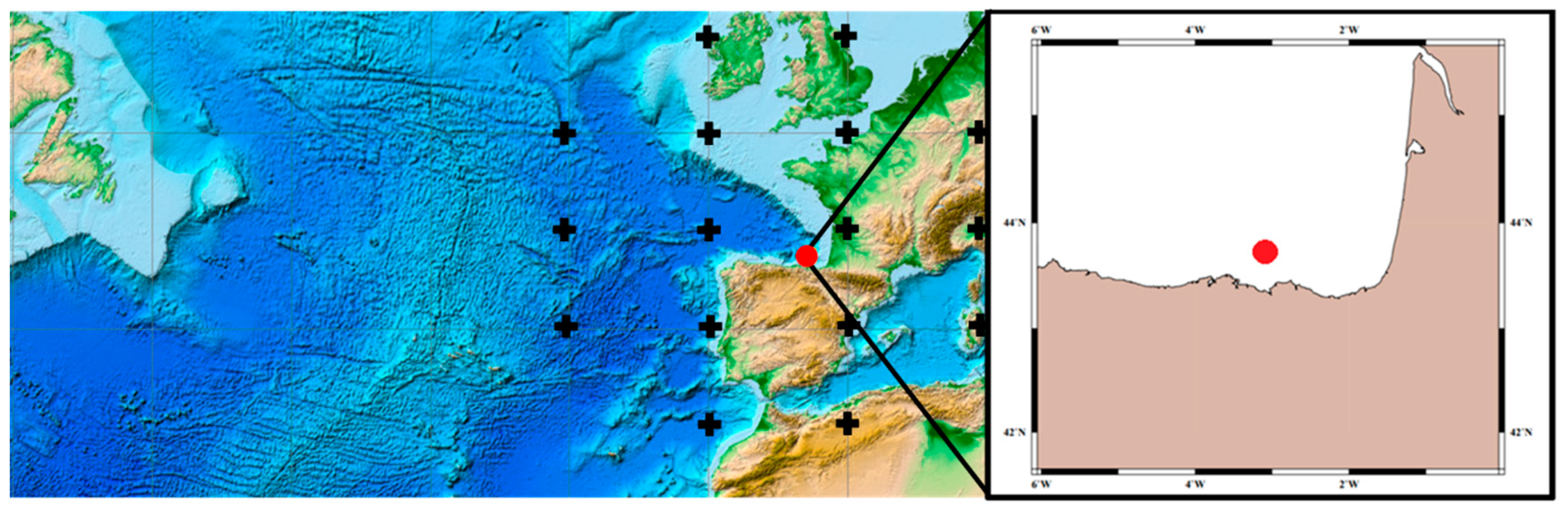
The study area is the south-easternmost corner of the Bay of Biscay, off the Spanish coast (Figure 1). This sector is characterized by a rugged but diverse coastline: cliffs and rocky coasts are dominant, but sandy beaches and wetlands are also present. At the present, most of the coast is classified as slightly erosive, although scattered signs of retreat are evident [17,18,19]. The coastal municipalities concentrate approximately 75% of the population and contribute up to 80% of the regional GDP. As a consequence, this region is strongly affected by extreme events, and the storm events are of great economic impact [20].
Data used in this research come from several sources (Table 1). Observed wave records (significant wave height (Hs), wave period (Tp), and wave direction (θ)) were obtained from the directional Bilbao-Vizcaya buoy (3.09° W; 43.64° N, mooring depth 870 m), belonging to the REDEXT network of Puertos del Estado. This buoy provided three-hourly values from 1991 to 1996, and hourly values onwards; thus, in order to work with a homogeneous temporal sampling, only the data from 1997 to 2015 were analyzed. Moreover, the original time series were filtered with a 6 h moving average for consistency with the temporal resolution (6-hourly) of the model outputs. The latter consists of a hindcast wave dataset, provided by Dr. Gillaume Dodet and was obtained from the third-generation spectral wave model WAVEWATCH III, forced with the 6-hourly wind fields of the NCEP (National Centers for Environmental Prediction) /NCAR (National Center for Atmospheric Research) Reanalysis 1 project, from January 1948 to March 2015 (for details regarding the modeling approach, please see Masselink et al. [22]). Only significant wave height was retrieved from the hindcast wave dataset.
Although hindcast wave data are useful to for analyzing long-term trends and large spatial patterns, particularly in deep waters, the coarse resolution of the original wind fields prevents the reproduction of the complete spectrum of the observed wave variability. Consequently, observed values were preferred for deriving a classification for coastal storms, based on the measured wave characteristics, whereas the long-term wave variability was analyzed using the closest grid point to the buoy from the hindcast output. Nevertheless, to assess the model skill, simulated significant wave height values were compared to the observed record through the calculation of some statistics. Moreover, some derived storm parameters were also evaluated for both datasets (namely, the number of storms and the duration).
The various methods of evaluating the storminess of a coastal region can be summarized in two main approaches, both used in this paper: (1) statistical and (2) climatological [23]. The statistical approach objectively quantifies coastal storm variability by applying a procedure that includes the definition and identification of individual storms, the choice of the parameters to characterize them, and the classification of the storms. Since so far there is no universally accepted definition for storm, a location-specific criterion that simplifies the extraction and comparison of storminess indices across several datasets was applied [24]. As a result, a storm occurs when the Hs values are greater than the 95th percentile of the daily maximum Hs (4.3 m) for both datasets, provided that, at least one record exceeds the 99th percentile of the daily maximum Hs (6.2 m). In order to identify statistically independent storms, the interval between two consecutive storms (storm peak to storm peak) should not be less than 36 h; otherwise, they are regarded as the same storm. Once a storm is identified, several indices are obtained to characterize its relevant properties: duration (number of records exceeding the aforementioned 95th percentile, assuming a minimum duration of 12 h, equaling the mesotidal cycle of the sea level along the coast of northern Spain); Hs, Tp, and wave direction during the storm peak; and the Storm Power Index (SPI) [25]. This latest index provides an approximation of the intensity, and consequently, the potential hazards that are induced by a storm. It is defined by the following equation:
where Hs is the significant wave height and td is the duration of the storm in hours.
SPI = ∑ Hs2 td
The atmospheric environment associated with wave storms (synoptic climatological approach) was examined by two complementary approaches. The first followed an Eulerian approach, which considers the passing of air particles through fixed points, and uses the surface pressure values around a selected region to quantify the atmospheric conditions by the estimation of several atmospheric indices (e.g., zonal (U) and meridional (V) wind components, and the strength of the geostrophic flow and the vorticity [21]). The second approach used a Lagrangian methodology, based on the tracking of extratropical cyclone pressure minimums and the calculation of some output variables [26] like, among others, the date (at 6-h intervals), the position (latitude and longitude) of each cyclone, and sea level pressure—in hPa—at the cyclone center (depth). The distance from the buoy to the center of each cyclone (in km) was derived through the Haversine’s formulae. A cyclone activity index (CAI) [27] was calculated from a square box of 10° size centered at 5° W, 55° N, as Iy = CyLy, where C is the number of cyclones observed during each winter in year y, and L is the temporal average of the local sea level pressure Laplacian. In both cases, the raw pressure values used as input were extracted from NCEP/NCAR Reanalysis 1 [28]. When pairing storms with atmospheric information for the region of interest, we followed an environment-to-circulation approach [29]: first, storms were identified, and after that, atmospheric configurations associated with the extreme local wave storms were subsequently determined. To do so, observed storms from the period of 1997 to 2015 (characterized by their values of Hs, Tp, wave direction at the storm peak, and total SPI released during the whole episode) and simultaneous atmospheric variables (local sea level pressure, zonal and meridional wind component, vorticity, distance, and depth of the cyclones) were arranged together and subjected to a cluster analysis to identify and group them into homogeneous sets. To minimize the large differences in variance, a prior standardization was performed to the original variables, and Ward’s hierarchical algorithm was used, which avoids the “snowball effect” upon small samples [30].
Monthly values of the most active patterns for the north Atlantic region (North Atlantic Oscillation—NAO, Eastern Atlantic—EA, Eastern Atlantic/Western Russia—EA/WR, and Scandinavian—SCAND) were downloaded from the Climate Prediction Center (http://www.cpc.ncep.noaa.gov/products/precip/CWlink/daily_ao_index/teleconnections.shtml) and the West Europe Pressure Anomaly (WEPI) index were used to assess the connection between wave storms, atmospheric parameters, and large scale circulation patterns. The West Europe Pressure Anomaly (WEPI) index was calculated as the difference between sea level pressure records of Valentia (Ireland) and Santa Cruz de Tenerife (Canary Islands, Spain) [31]. All monthly records were averaged into seasonal values. Quantification of the relationships was made using the non-parametric Spearman rank correlation coefficient, which is recommendable for data that is not normally distributed. The statistical significance of the long-term trends in storminess and atmospheric variability was revised by the means of robust, non-parametric methods, the Sen’s slope estimator [32] and the Mann-Kendall test, to figure out the change per unit time of the observed trends, as well as the sequential version of the Mann-Kendall test [33], to detect change points in long-term time series. In this version, a normalized Kendall tau was calculated either from the beginning (end) of the time series, conforming to a progressive u(t) or a retrograde u’(t) series; points where both series crossed themselves were considered to be approximate potential trend turning points. When either the progressive or the retrograde values exceeded certain confidence limits before and after the crossing points, the trend was considered to be significant at a pre-established significance level. Autocorrelations were computed for all the time series at varying time-lags, checking for randomness. As all lag-1 serial correlation coefficients were statistically not significant, there was no need to pre-white the data; thus, the statistical tests described above were applied to the original time series [34].
3. Results
3.1. Identification, Characterization, and Classification of Extreme Wave Events
As stated in the methodology section, we first performed a comparison between the observed and modelled data to validate the reliability of hindcast data in the study area. Simulated and measured significant wave heights showed an overall good agreement, with an R2 of 0.83, a BIAS of 1.2 cm and a RMSE (Root Mean Square Error) of 37 cm, although in general, the model slightly underestimated the measurements (Figure 2, left). Comparisons between the annual number of storms and their duration also presented a good agreement between the modelled and the observed measurements (Figure 2, right). A total of 50 (44) storms were identified in the observed (hindcast) record between 1997 and 2015 (meaning less than three storms per year on average), spanning through 339 h (367). Since most of the storms occurred during the winter months (73%), henceforth, we focused the analysis on this season, spanning the months of December, January, and February.
The next task consisted of an exploratory analysis of the role of the atmospheric circulation upon the characteristics of the storms. It was expected that intense cyclones are the cause of extreme wave events, particularly on non-fetch-limited sea environments that are exposed to the propagation of swell through the ocean [35]. So, to confirm whether some characteristics of the extreme wave events depended on the properties of extratropical cyclones, the wave height and the period of each event were correlated, at the peak of each storm, against duration, the energy released, and the simultaneous location and depth of the forcing cyclone. It was clear that the depth of the cyclone and its distance to the buoy became more important for the wave period. Besides, longer and more energetic events corresponded to higher wave heights and periods (Table 2).
The following step was to identify homogeneous structures within the observed storm database. Attributes included in the classification procedure were a combination of oceanographic and atmospheric variables, whose resulting class-averaged values for each storm type, as well as their level of significance according to a non-parametric Kruskall-Wallis test, are presented in Table 3. Cluster 1 (28 storms) was characterized by storms with a longer duration and energy, a longer wave period, a counterclockwise wave direction, a stronger zonal wind flow and distant but deeper cyclones. On the contrary, storms belonging to Cluster 2 (35 storms) were characterized by wave heights of similar values but shorter periods, less duration and energy, a clockwise wave direction, the predominance of a meridional cyclonic flow, and closer but shallower cyclones. The variables offering the greatest discrimination capability were wave period, the duration and SPI of the storm, zonal and the meridional wind component, vorticity, depth, and the distance to the cyclone.
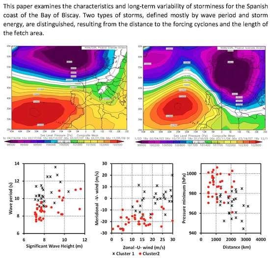
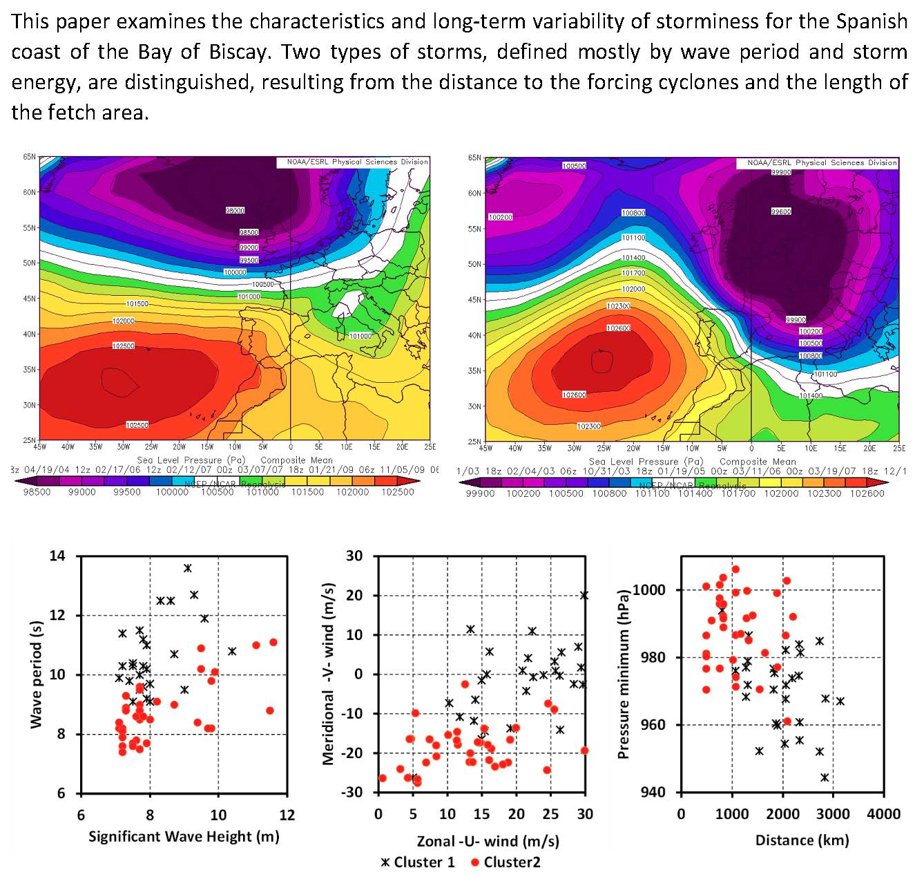
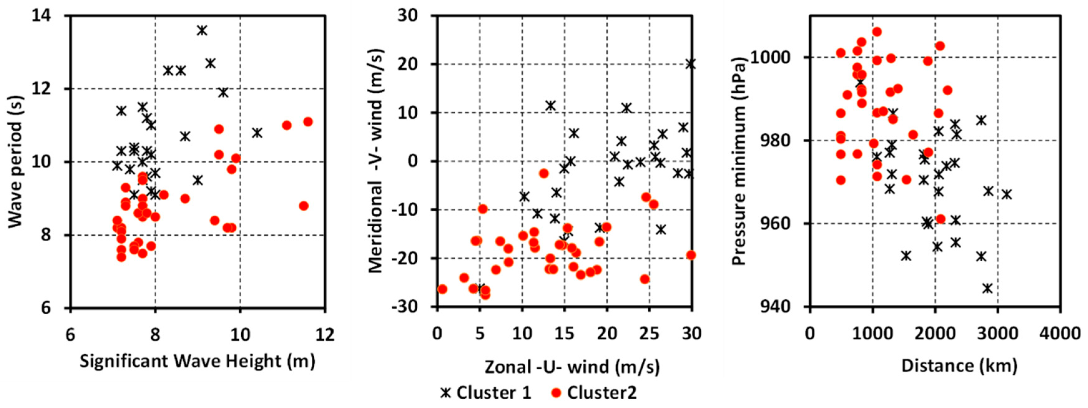
Figure 3 provides scatterplots displaying the nature of the relation between selected pairs of variables. For example, the quality of the partition between wave height and period in the data space was not good (Figure 3, left). Nonetheless, for most of the Cluster 1 events, the wave period is larger than 10 s, contrary to the distribution from Cluster 2. Concerning the behavior of the wave height, there was no difference between both clusters below 10 m, but, beyond that threshold, the majority of the events belonged to Cluster 2. Higher differentiation showed both zonal and meridional wind components (Figure 3, center). High zonal wind values and close to 0 V values represented the dominance of westerly (W) to northwesterly (NW) winds in the Cluster 1 storms; conversely, Cluster 2 storms showed negative values of the V wind component and neutral to low positive values of the U wind component, meaning NW to N winds. Finally, readers can observe the relationship between the position and the depth of the storm in Figure 3 (right). The depths of the cyclones corresponding to storms that were classified as Cluster 2 were shallower than 980 hPa, while their distances to the buoy were lower than 2000 km. On the contrary, Cluster 1 was characterized by much deeper (less than 980 hPa), but distant lows. It seems that, in terms of significant wave height, deeper but distant lows compensate for the effect of closer but shallower lows. However, if intensity and proximity meet, as for example, during the crossing of “meteorological bombs” like cyclone “Klaus”, significant wave heights reach exceptional values. On the days of that event, the Bilbao-Vizcaya buoy recorded a peak of 13.71 m as a significant wave height, simultaneous to a sea level pressure minimum (978.9 hPa). Another buoy moored close to the city of Santander broke off its clamping system and drifted eastward over three days, and was finally found close to the French coast.
3.2. Atmospheric Controls Upon Wave Storms
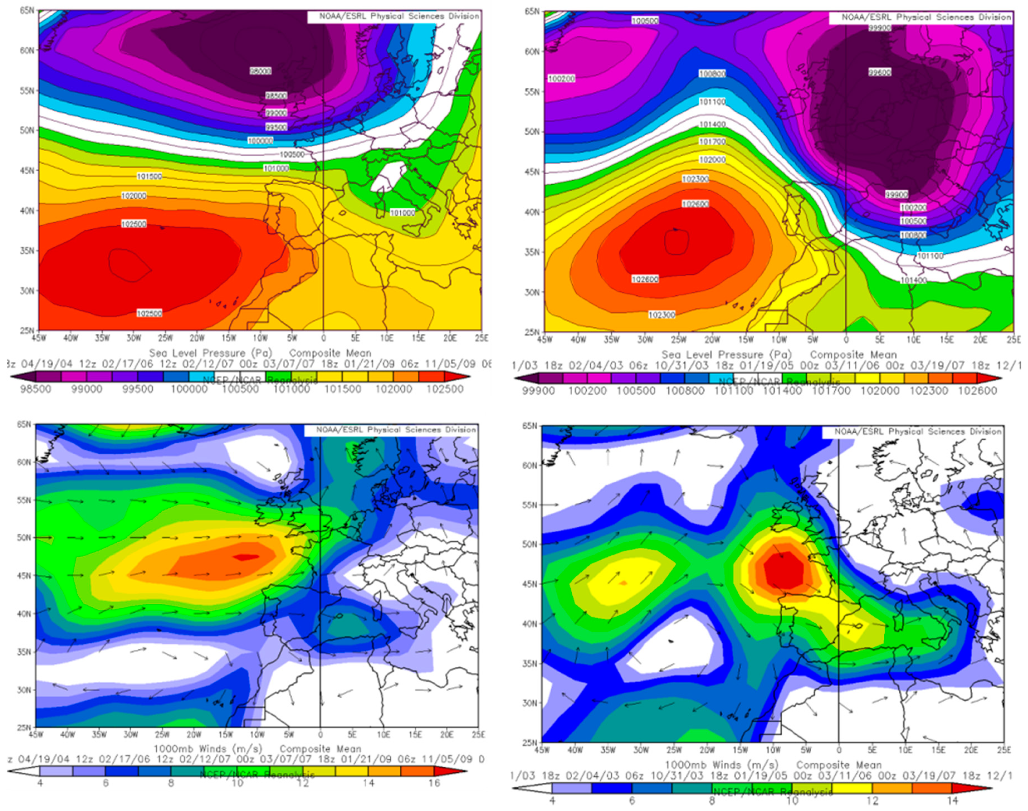
In order to confirm that different anomalous circulation patterns support each cluster, a composite analysis of sea level pressure and wind fields, corresponding with all of the storms of each cluster, during the period of analysis (1997–2015) was performed (Figure 4). As suggested by the results observed in Table 3, Cluster 1 depicts a large scale zonal pressure gradient, covering most of the eastern Atlantic basin, between a strong Azores High and a deep low pressure area, which is located beyond the 55° N parallel. The area of the stronger winds, which are responsible for the wave trains arriving to the northern coast of Spain, are located far away from the Iberian Peninsula. Conversely, a northwesterly flow, between a northeastern expanded Azores High and a low pressure area over Western Europe, characterizes Cluster 2. Much stronger winds are observed closer to the study area, and their predominant component is northwesterly.
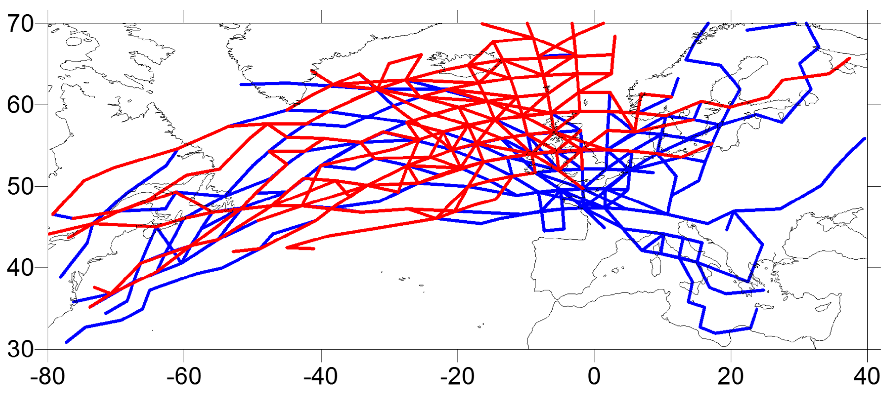
Since the location and depth of the cyclones seems to be the key parameter of this classification, we also had a look at the origin of the cyclones causing the wave storms, plotting their tracks along their life cycle (Figure 5). The most remarkable aspect was the beginning of bifurcation of the storm tracks approximately at the 10° W meridian. Although most of the cyclones that cause storms in the Bay of Biscay area are originated along the well-known cyclogenesis area of the eastern seaboard of Northern America, when arriving to the aforementioned meridian, some of them (Cluster 1) follow a SW-NE track to the Norway Sea, meanwhile others (Cluster 2) divert to a SE track, heading to central Europe. Furthermore, it is not unusual that some cyclones that are classified within Cluster 2 are the result of secondary cyclogenesis in the SE margin of deeper Atlantic storms which follow a similar track to Cluster 1.
3.3. Analysis of Long-Term Variability in Storminess
Due to the good correspondence between observed and modelled data in terms of significant wave height, we considered an extension of the analysis for the period 1948–2015. Thus, a retrospective analysis of storminess in the Bay of Biscay area using the same criteria as before (Section 3.1) was accomplished by calculating the number of storms and their SPI from the modelled data. However, it was not possible to replicate a similar clustering procedure for the complete period 1948–2015 using the modelled data, because of the poorer correspondence between the observed and modelled wave periods (not shown). Since the wave period is more discriminant than the wave height in defining each cluster, it was not recommendable to extend our clustering procedure based on a variable that was not satisfactorily resolved by the model. Alternatively, we analyzed the long-term evolution (1948–2015) of the atmospheric forcing upon each cluster by selecting and counting, for the study area and at 6-hourly time steps, those atmospheric fields that fulfilled several criteria that were derived from the previous clustering. To do so, quantitative thresholds were obtained for selected atmospheric variables (sea level pressure, zonal, and meridional wind, and vorticity, plus cyclone pressure minimum and cyclone distance), extracted from the NCEP1 Reanalysis. At each 6-hour time-step, we looked for the simultaneous fulfilling of the criteria. When such conditions were found, it was considered to be a high probability of occurrence of an “event”, either Cluster 1 or Cluster 2, depending on the criteria used. Additionally, the CAI time series corresponding to the area of the most frequent bifurcation of the storm tracks (a 10° square box centered at 5° W, 55° N) were also calculated.
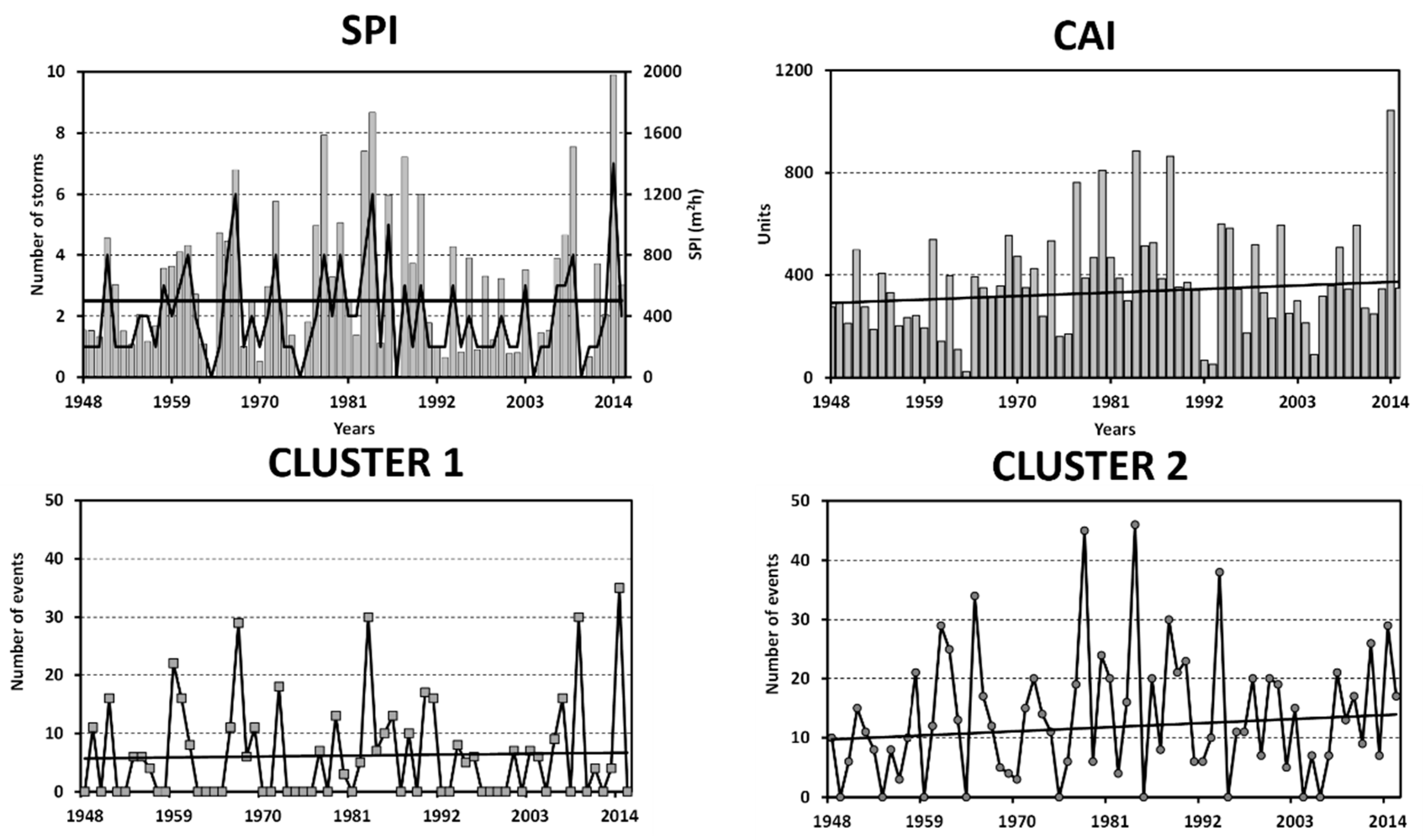
Since 1948, on average, three storms struck the study area each year, but this figure hid remarkable inter-annual variability (Figure 6). Four winters did not register any storm (1964, 1975, 1987, 2004, and 2010), while another other four winters (1967, 1984, 1986 and 2014) suffered at least five storms. There was no an exact match between the ranking of years by the number of storms with the ranking of years that were ordered by SPI. For example, 1984 was the second stormiest season in both indices (six storms and 1735 m2 h), 1978 and 2009 experienced only four storms but more energetic conditions (1585 and 1509 m2 h) than 1967 and 1986 (1360 and 1194 m2 h) in which five and six storms occurred, respectively. At the end of the time series, the exceptional stormy winter season of 2013–2014 was evident, due more to a higher number of storms rather than the energy released (seven storms and 1978 m2 h). The strong cyclonic circulation around the British Isles during that winter was clearly visible in the plots representing the CAI and the number of observations matching Cluster 1.
The analysis carried out by means of the Sen’s test did not yield significant results (Table 4). Values of the z-statistic and the slope of the best fit line were low, and even in the case of the SPI index, the latter was virtually flat. Those results were additionally checked with a Spearman’s rank test in order to enhance the reliability of trend outputs, but the results were almost the same.
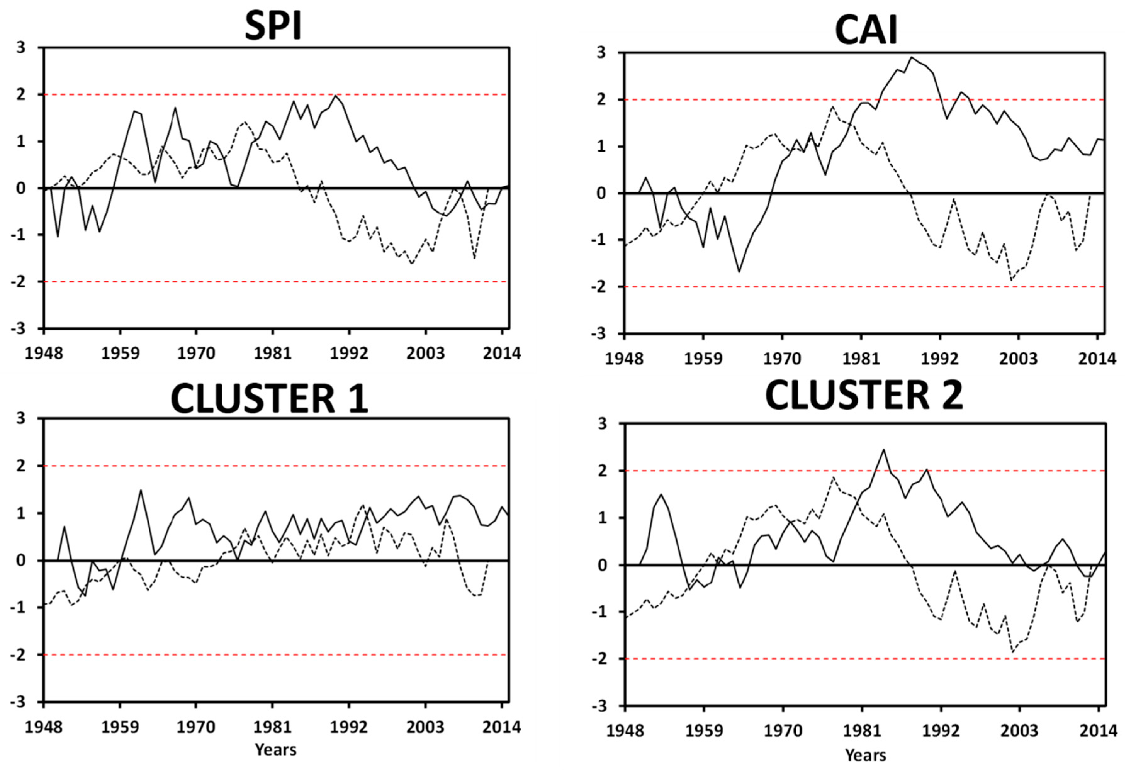
The values of u(t) and u’(t), both derived from the sequential Mann-Kendall test, are depicted by solid and dashed lines (Figure 7). Through the calculation of a progressive and a retrograde series of Kendall normalized tau’s, the crossing of the two lines were considered as approximate potential trend turning points. When either the progressive or retrograde rows exceeded certain confidence limits before and after the crossing points, those trend turning points were considered to be significant at the corresponding level. Except for Cluster 1, the other time series displayed a common behavior, exhibiting an increase up to the end of the 1980s (the change occurred in 1984, 1988, or 1990, depending on the time series), and a decrease afterwards, with stabilization during the initial years of the 21st century. This increasing trend was statistically significant at a 95% confidence level for SPI, CAI, and Cluster 2. The beginning of such a trend, as marked by the intersection point of u(t) and u’(t) curves, was less clear, but was established to be around the beginning of the 1960s. The graphical representation of u(t) and u’(t) for Cluster 1 did not show any trend; rather, both curves overlapped several times.
The position and strength of the Atlantic storm track activity is strongly coupled to some large-scale teleconnection patterns, such as the NAO [36,37]. The degree of control exerted by those low frequency patterns upon the wave storms, the meteorological conditions prone to them, and the cyclone tracks, were assessed though a simple correlation analysis. A Spearman rank correlation procedure between the seasonal indices of NAO, EA, EA/WR, SCAND, and WEPI, against the seasonal values of number of storms, SPI, CAI, and the frequency of the occurrence of Cluster 1 and Cluster 2 storms, was carried out (Table 5). The most significant correlations were obtained from WEPI, which is a regionally customized index used to enhance the atmospheric signal related to wave storms over the Bay of Biscay area. The other indices, whose spatial scales were hemispheric, at least, displayed weaker correlations. The most active was the EA/WR pattern, which displays significant, but moderate, correlations with all wave and atmospheric indices, except with the frequency of Cluster 1 storms. The other patterns only displayed occasional correlations with one or two indices; for example, the EA pattern with CAI and Cluster 1 storms, while NAO only showed a positive but weak correlation with the Cluster 2 storms, as well as SCAND with CAI.
4. Discussion
Since storminess is a key issue in coastal erosion and climate change studies, characteristics and temporal evolution of wave storms along the Spanish coast of the Bay of Biscay area are the main subject of our analysis. The first task was accomplished using observed data from Bilbao-Vizcaya buoy, covering the period 1997–2015; meanwhile, a hindcast database, spanning from 1948–2015, was used for the second task after checking the reliability of the latter.
Since our interest is to highlight the relationship between coastal storms and atmospheric forcing, we first applied a statistical procedure to identify and characterize storms, and secondly, a clustering to group them into different types. The attributes subject to grouping did not exclusively include local wave parameters, but also atmospheric variables that reproduced large scale processes. Such procedures allowed us to recognize two types of storms in response to extratropical cyclones that follow different tracks. Sea states corresponding to each class are mainly distinguished by the wave period and wave energy; distant cyclones produce higher wave periods, more westerly waves, and more energetic conditions (swell conditions) than closer cyclones (mixed swell and wind sea states). The current approach differs from other methodologies applied to identify and characterize energetic wave conditions. One example is the use of unsupervised clustering algorithms to group wave data into a few sea-state modes, each of them being associated with contrasted values for wave height, period, and direction [38,39]. Other approaches [40,41] that focus on the potential effect of storms upon coastlines, categorized storms into several classes on the basis of the energy content for each storm, but the link between wave storminess and large scale circulation is less evident than in our approach.
Subsequently, the long-term evolution of storminess, quantified by the SPI calculated from hindcast data, was compared with the evolution of the large scale circulation. We have not found any significant trends, although substantial interannual and decadal variability is present. The most active period of storminess spanned the second half of the 1970s and the 1980s; the decades following that maximum experienced a reduced activity, as well as in the initial years of the time series.
Those stormy seasons do not coincide with studies on storminess along other Atlantic regions of the Iberian Peninsula; rather, the Bay of Biscay area shares a common temporal behavior with northerly latitudes. The most intense stormy seasons in the Gulf of Cadiz area were 2010, 1963, and 1996, when cyclones followed a southerly-displaced track, which was related to the negative phases of the NAO [42,43]. Storm variability along the northern coast of Spain closely resembles the storm activity north of 55° N: low during the 1950s, increased through the 1960s, and peaking in the early 1990s, before decreasing until 2014 [44,45,46,47]. Such a trend was part of a decadal variability which, at secular time scales, does not show a trend in storm numbers.
An interesting feature is the occurrence of the exceptional winter of 2013–2014, at the end of the period of analysis, which offered record-breaking numbers of storms, wave energy, cyclonic activity, and morphological impacts on the coast of France and the UK [48,49]. Analysis is underway on the effects of those storms during the winter of 2014, which also offer a picture of extraordinary damage along the northern coast of Spain in both the natural environment, and on infrastructure and equipment, the restoration of which was worth around €70 million [20].
Finally, we have confirmed the relevance of the recent WEPI patterns for wave storms, Energy, and related cyclonic activity along the northern coast of the Iberian Peninsula; however, the correlation values that are obtained are lower in comparison with the French coastline [31]. The underlying reason is that many storms that hit the Spanish coast need a more northerly component of the large scale flow (Cluster 2), while the French coast is open to storms with a zonal component (Cluster 1 [50]). In the case of other “classical” teleconnections patterns, the EA/WR pattern is most relevant for the occurrence of wave storms along the northern coast of Spain, mostly linked to Cluster 2; the negative sign of the correlation between the seasonal value of the EA/WR index and the SPI reflects the association between wave storms and negative tropospheric height anomalies over Western Europe. The EA pattern, related to Cluster 1, as well as the NAO pattern (Cluster 2) does not show significant correlations with wave storminess. In that sense, these results are not in total agreement with previous publications, since, for example. Dodet et al. [5] found weak to strong correlations between winter NAO indices and the annual 90th percentile of wave heights, while Charles et al. [10] and Le Cozannet et al. [14] also found a strong and direct correlation between the NAO and EA indices, and high-energy waves. Again, we think that the orientation of the coast in both sides of the Bay of Biscay can explain such a disagreement.
Coastal erosion depends not only on the energy released by the storms, derived from significant wave height, but also from other attributes, such as the storm duration, the clustering of successive storms, or the incidence angle with which the wave trains hit against the coastline. Climate scenarios at the basin scale show that global warming might lead to an eastward extension of the North Atlantic storm track [51,52]. However, such evolution will offer substantial regional variability due to a complex association of processes working at different spatial and temporal scales. For example, an intensification and northeastward shift of strong wind core in the North Atlantic Ocean will induce a clockwise shift of winter swell directions along the Bay of Biscay [53]. Such changes would impact the coastal dynamics, modifying the rates of accretion or erosion, by reducing the long-shore sediment flux.
5. Conclusions
An analysis of storminess at the northern coast of Spain reveals two different atmospheric forcings, one mixing swell and wind seas, and another characterized by predominant wind sea conditions. The evolution of storminess and their forcing mechanisms during the period 1948–2015 does not show significant temporal trends, but a decadal variability associated with fluctuations in the WEPI, EA, and EA/WR large scale teleconnection patterns. The greatest storm activity occurred between 1960 and 1980, although the winter of 2013–2014 experienced by far the longest and more intense sequence of storms in the record.
Author Contributions
Conceptualization and Methodology, D.R.; Formal Analysis, D.R.; Investigation, Writing-Original Draft Preparation, Writing-Review & Editing, Visualization, Supervision, Funding Acquisition, all authors.
Funding
This paper has been possible within the framework of the research project 17.JU11.64661 “Climatología Histórica de temporales en el área cantábrica (1851–2015)”, funded by SODERCAN S.A. (Sociedad para el Desarrollo Regional de Cantabria) and Programa Operativo FEDER, and the support of Biodiversity Foundation of the Ministry for Ecological Transition of Spain.
Acknowledgments
The authors express their gratitude to Guillaume Dodet. from Université de Bretagne Occidentale for the provision of the modelled wave database, and Puertos del Estado, provider of the Bilbao-Vizcaya buoy database.
Conflicts of Interest
The authors declare no conflict of interest. The founding sponsors had no role in the design of the study; in the collection, Analyses, or interpretation of data; in the writing of the manuscript, and in the decision to publish the results.
References
- Morton, R.A.; Gibeaut, J.C.; Paine, J.G. Meso-scale transfer of sand during and after storms: Implications for prediction of shoreline movement. Mar. Geol. 1995, 126, 161–179. [Google Scholar] [CrossRef]
- Bouws, E.; Jannink, D.; Komen, G.J. The increasing wave height in the North Atlantic Ocean. Bull. Am. Meteorol. Soc. 1996, 77, 2275–2277. [Google Scholar] [CrossRef]
- Woolf, D.K.; Challenor, P.G.; Cotton, P.D. Variability and predictability of the North Atlantic wave climate. J. Geophys. Res. 2002, 107, 3145. [Google Scholar] [CrossRef]
- Izaguirre, C.; Méndez, F.J.; Menéndez, M.; Losada, I.J. Global extreme wave height variability based on satellite data. Geophys. Res. Lett. 2011, 38. [Google Scholar] [CrossRef] [Green Version]
- Dodet, G.; Bertin, X.; Taborda, R. Wave climate variability in the North-East Atlantic Ocean over the last six decades. Ocean Model. 2010, 31, 120–131. [Google Scholar] [CrossRef]
- Semedo, A.; Suselj, K.; Rutgersson, A.; Sterl, A. A global view on the wind sea and swell climate and variability from ERA-40. J. Clim. 2011, 24, 1461–1479. [Google Scholar] [CrossRef]
- Bertin, X.; Prouteau, E.; Letetrel, C. A significant increase in wave height in the North Atlantic Ocean over the 20th century. Glob. Planet. Chang. 2013, 106, 77–83. [Google Scholar] [CrossRef]
- Castelle, B.; Dodet, G.; Masselink, G.; Scott, T. Increased winter-mean wave height, variability, and periodicity in the northeast Atlantic over 1949–2017. Geophys. Res. Lett. 2018, 45, 3586–3596. [Google Scholar] [CrossRef]
- Dupuis, H.; Michel, D.; Sottolichio, A. Wave climate evolution in the Bay of Biscay over two decades. J. Mar. Syst. 2006, 63, 105–114. [Google Scholar] [CrossRef]
- Charles, E.; Idier, D.; Thiebot, J.; Le Cozannet, G.; Pedreros, R. Present wave climate of the Bay of Biscay: Spatiotemporal variability and trends from 1958 to 2001. J. Clim. 2012, 25, 2020–2039. [Google Scholar] [CrossRef]
- Paris, F.; Lecacheux, S.; Idier, D.; Charles, E. Assessing wave climate trends in the Bay of Biscay through an intercomparison of wave hindcasts and reanalyses. Ocean Dyn. 2014, 64, 1247–1267. [Google Scholar] [CrossRef]
- Lerma, A.N.; Bulteau, T.; Lecacheux, S.; Idier, D. Spatial variability of extreme wave height along the Atlantic and channel French coast. Ocean Eng. 2015, 97, 175–185. [Google Scholar] [CrossRef]
- Ulazia, A.; Penalba, M.; Ibarra-Berastegui, G.; Ringwood, J.; Saénz, J. Wave energy trends over the Bay of Biscay and the consequences for wave energy converters. Energy 2017, 141, 624–634. [Google Scholar] [CrossRef]
- Le Cozannet, G.; Lecacheux, S.; Delvallée, E.; Desramaut, N.; Oliveros, C.; Pedreros, R. Teleconnection pattern influence on sea-wave climate in the Bay of Biscay. J. Clim. 2011, 24, 641–652. [Google Scholar] [CrossRef]
- Bromirski, P.D.; Cayan, D.R. Wave power variability and trends across the North Atlantic influenced by decadal climate patterns. J. Geophys. Res. Oceans 2015, 120, 3419–3443. [Google Scholar] [CrossRef] [Green Version]
- Martínez-Asensio, A.; Tsimplis, M.N.; Marcos, M.; Feng, X.; Gomis, D.; Jordà, G.; Josey, S.A. Response of the North Atlantic wave climate to atmospheric modes of variability. Int. J. Climatol. 2016, 36, 1210–1225. [Google Scholar] [CrossRef]
- Rivas, V.; Cendrero, A. Human influence in a low-hazard coastal area: An approach to risk assessment and proposal of mitigation strategies. J. Coast. Res. 1994, SI 12, 289–298. Available online: https://www.jstor.org/ stable/25735605 (accessed on 14 June 2018).
- García Codron, J.C.; Rasilla Álvarez, D.F. Coastline retreat, sea level variability and atmospheric circulation in Cantabria (Northern Spain). J. Coast. Res. 2006, SI 48, 49–54. Available online: https://www.jstor.org/stable/25737381 (accessed on 14 June 2018).
- Chust, G.; Caballero, A.; Marcos, M.; Liria, P.; Hernández, C.; Borja, Á. Regional scenarios of sea level rise and impacts on Basque (Bay of Biscay) coastal habitats, throughout the 21st century. Estuar. Coast. Shelf Sci. 2010, 87, 113–124. [Google Scholar] [CrossRef] [Green Version]
- Garmendia Pedraja, C.; Rasilla Álvarez, D.F.; Rivas Mantecón, V. Distribución espacial de los daños producidos por los temporales de invierno 2014 en la costa norte de España: Peligrosidad. vulnerabilidad y exposición. Estudios Geográficos 2017, 78, 71–104. [Google Scholar] [CrossRef]
- Jenkinson, A.F.; Collison, F.P. An Initial Climatology of Gales over the North Sea. In Synoptic Climatology Branch Memorandum, No. 62; Meteorological Office: Bracknell, UK, 1977. [Google Scholar]
- Masselink, G.; Castelle, B.; Scott, T.; Dodet, G.; Suanez, S.; Jackson, D.; Floc’h, F. Extreme wave activity during 2013/2014 winter and morphological impacts along the Atlantic coast of Europe. Geophys. Res. Lett. 2016, 43, 2135–2143. [Google Scholar] [CrossRef] [Green Version]
- Ciavola, P.; Coco, G. Coastal Storms: Processes and Impacts; John Wiley & Sons Ltd.: Hoboken, NJ, USA, 2017. [Google Scholar]
- Zhang, K.; Douglas, B.C.; Leatherman, S.P. Twentieth-Century Storm Activity along the U.S. East Coast. J. Clim. 2000, 13, 1748–1761. [Google Scholar] [CrossRef]
- Dolan, R.; Davis, R.E. An Intensity Scale for Atlantic Coast Northeast Storms. J. Coast. Res. 1992, 8, 840–853. [Google Scholar]
- Serreze, M.C. Climatological aspects of cyclone development and decay in the Arctic. Atmos. Ocean 1995, 33, 1–23. [Google Scholar] [CrossRef] [Green Version]
- Wang, X.L.; Swail, V.R.; Zwiers, F.W. Climatology and Changes of Extratropical Cyclone Activity: Comparison of ERA-40 with NCEP–NCAR Reanalysis for 1958–2001. J. Clim. 2006, 19, 3145–3166. [Google Scholar] [CrossRef]
- Kalnay, E.; Kanamitsu, M.; Kistler, R.; Collins, W.; Deaven, D.; Gandin, L.; Iredell, M.; Saha, S.; White, G.; Woollen, J.; et al. The NCEP/NCAR 40-Year Reanalysis Project. Bull. Am. Meteorol. Soc. 1996, 77, 437–472. [Google Scholar] [CrossRef]
- Yarnal, B. Synoptic Climatology in Environmental Analysis; Belhaven Press: London, UK, 1993. [Google Scholar]
- Wilks, D. Statistical Methods in the Atmospheric Sciences; International Geophysics Series; Academic Press: New York, NY, USA, 2011; Volume 100, Available online: https://www.sciencedirect.com/bookseries/international-geophysics/vol/100 (accessed on 9 August 2018).
- Castelle, B.; Dodet, G.; Masselink, G.; Scott, T. A new climate index controlling winter wave activity along the Atlantic coast of Europe: The West Europe Pressure Anomaly. Geophys. Res. Lett. 2017, 44, 1384–1392. [Google Scholar] [CrossRef] [Green Version]
- Sen, P.K. Estimates of the regression coefficient based on Kendall’s Tau. J. Am. Stat. Assoc. 1968, 63, 1379–1389. [Google Scholar] [CrossRef]
- Sneyers, R. On the Statistical Analysis of Series of Observations; World Meteorological Organization (WMO): Geneva, Switzerland, 1990; No. 143; Available online: https://library.wmo.int/pmb_ged/wmo_415.pdf (accessed on 14 June 2018).
- Luo, Y.; Liu, S.; Fu, S.; Liu, J.; Wang, G.; Zhou, G. Trends of precipitation in Beijiang River Basin. Guangdong Province. China. Hydrol. Process. 2008, 22, 2377–2386. [Google Scholar] [CrossRef]
- Bell, R.J.; Gray, S.L.; Jones, O.P. North Atlantic storm driving of extreme wave heights in the North Sea. J. Geophys. Res. Oceans. 2017, 122, 3253–3268. [Google Scholar] [CrossRef] [Green Version]
- Marshall, J.; Kushnir, Y.; Battisti, D.; Chang, P.; Czaja, A.; Dickson, R.; Hurrell, J.; McCartney, M.; Saravanan, R.; Visbeck, M. North Atlantic climate variability: Phenomena, impacts and mechanisms. Int. J. Climatol. 2001, 21, 1863–1898. [Google Scholar] [CrossRef] [Green Version]
- Trigo, R.M.; Valente, M.A.; Trigo, I.F.; Miranda, P.M.; Ramos, A.M.; Paredes, D.; García-Herrera, R. The Impact of North Atlantic Wind and Cyclone Trends on European Precipitation and Significant Wave Height in the Atlantic. Ann. N. Y. Acad. Sci. 2008, 1146, 212–234. [Google Scholar] [CrossRef] [PubMed]
- Butel, R.; Dupuis, H.; Bonneton, P. Spatial variability of wave conditions on the French Atlantic coast using in-situ data. J. Coast. Res. 2002, SI 36, 96–108. [Google Scholar] [CrossRef]
- Bertin, X.; Castelle, B.; Chaumillon, E.; Butel, R.; Quique, R. Longshore transport estimation and inter-annual variability at a high-energy dissipative beach: St. Trojan beach. SW Oléron Island. France. Cont. Shelf Res. 2008, 28, 1316–1332. [Google Scholar] [CrossRef]
- Mendoza, E.T.; Jimenez, J.A.; Mateo, J. A coastal storms intensity scale for the Catalan sea (NW Mediterranean). Nat. Hazards Earth Syst. Sci. 2011, 11, 2453–2462. [Google Scholar] [CrossRef] [Green Version]
- Rangel-Buitrago, N.; Anfuso, G. Winter wave climate. storms and regional cycles: The SW Spanish Atlantic coast. Int. J. Climatol. 2013, 33, 2142–2156. [Google Scholar] [CrossRef]
- Almeida, L.P.; Ferreira, O.; Vousdoukas, M.I.; Dodet, G. Historical variation and trends in storminess along the Portuguese South Coast. Nat. Hazards Earth Syst. Sci. 2011, 11, 2407–2417. [Google Scholar] [CrossRef] [Green Version]
- Plomaritis, T.A.; Benavente, J.; Laiz, I.; del Rio, R. Variability in storm climate along the Gulf of Cadiz: The role of large scale atmospheric forcing and implications to coastal hazards. Clim. Dyn. 2015, 45, 2499–2514. [Google Scholar] [CrossRef]
- Bacon, S.; Carter, D.J. A connection between mean wave height and atmospheric pressure gradient in the North Atlantic. Int. J. Climatol. 1993, 13, 423–436. [Google Scholar] [CrossRef]
- O’Connor, M.C.; Cooper, J.A.G.; Jackson, D.W.T. Decadal behavior of tidal inlet-associated beach systems, Northwest Ireland, in relation to climate forcing. J. Sediment. Res. 2011, 81, 38–51. [Google Scholar] [CrossRef]
- Feser, F.; Barcikowska, M.; Krueger, O.; Schenk, F.; Weisse, R.; Xia, L. Storminess over the North Atlantic and northwestern Europe—A review. Q. J. Roy. Meteorol. Soc. 2014, 141, 350–382. [Google Scholar] [CrossRef]
- Matthews, T.; Murphy, C.; Wilby, R.L.; Harrigan, S. Stormiest winter on record for Ireland and UK. Nat. Clim. Chang. 2014, 4, 738–740. [Google Scholar] [CrossRef] [Green Version]
- Masselink, G.; Scott, T.; Poate, T.; Russell, P.; Davidson, M.; Conley, D. The extreme 2013/2014 winter storms: Hydrodynamic forcing and coastal response along the southwest coast of England. Earth Surf. Process. Landf. 2016, 41, 378–391. [Google Scholar] [CrossRef]
- Robinet, A.; Castelle, B.; Idier, D.; Le Cozannet, G.; Déqué, M. Charles E. Statistical modeling of interannual shoreline change driven by North Atlantic climate variability spanning 2000–2014 in the Bay of Biscay. Geo-Mar. Lett. 2016, 36, 479–490. [Google Scholar] [CrossRef] [Green Version]
- Bengtsson, L.; Hodges, K.I.; Roeckner, E. Storm tracks and climate change. J. Clim. 2006, 19, 3518–3543. [Google Scholar] [CrossRef]
- Ulbrich, U.; Pinto, J.G.; Kupfer, H.; Leckebusch, G.C.; Spangehl, T.; Reyers, M. Northern Hemisphere storm tracks in an ensemble of IPCC climate change simulations. J. Clim. 2008, 21, 1669–1679. [Google Scholar] [CrossRef]
- Ulbrich, U.; Leckebusch, G.C.; Pinto, J.G. Extra-tropical cyclones in the present and future climate: A review. Theor. Appl. Climatol. 2009, 96, 117–131. [Google Scholar] [CrossRef]
- Charles, E.; Idier, D.; Delecluse, P.; Déqué, M.; Le Cozannet, G. Climate change impact on waves in the Bay of Biscay France. Ocean Dyn. 2012, 62, 831–848. [Google Scholar] [CrossRef]
Figure 1.
Location of the study area (left) and the Bilbao-Vizcaya buoy (right). Crosses on the left display the grid nodes used for the extraction of the atmospheric indices following the Jenkinson and Collison method (1977) [21]. A red dot on the right indicates the location of the Bilbao-Vizcaya buoy.

Figure 2.
Scatterplot of observed versus modelled significant wave height (left) and comparison between derived storm parameters on the observed and hindcast output (right). Bars are the number of storms, lines are the duration of storms, orange are observed data, and gray are modelled data.
Figure 2.
Scatterplot of observed versus modelled significant wave height (left) and comparison between derived storm parameters on the observed and hindcast output (right). Bars are the number of storms, lines are the duration of storms, orange are observed data, and gray are modelled data.

Figure 3.
Scatterplots representing atmospheric properties defined by cluster (left), significant wave height versus wave period (center), zonal wind component versus meridional wind component (right), and the distance of the forcing cyclone versus depth.
Figure 3.
Scatterplots representing atmospheric properties defined by cluster (left), significant wave height versus wave period (center), zonal wind component versus meridional wind component (right), and the distance of the forcing cyclone versus depth.

Figure 4.
Composite sea level pressure (upper row) and wind (lower row) fields corresponding to wave storms belonging to Cluster 1 (left column) and Cluster 2 (right column). Image provided by the NOAA/ESRL Physical Sciences Division, Boulder Colorado from their Web site at http://www.esrl.noaa.gov/psd/.

Figure 5.
Storm tracks corresponding to wave storms belonging to Cluster 1 (red) and Cluster 2 (blue).
Figure 5.
Storm tracks corresponding to wave storms belonging to Cluster 1 (red) and Cluster 2 (blue).

Figure 6.
Long-term (1948–2015) evolution of wave storminess and associated atmospheric indices. (Upper left) number of storms (bars) and SPI (black line); (upper right) the cyclone activity index (CAI) for the 10° box centered at 5° W, 55° N; (lower left) the number of events associated with Cluster 1; (lower right) the number of events associated with Cluster 2. Each plot includes the best fit line obtained from Sen´s method.

Figure 7.
Values of progressive (u(t), solid line) and retrograde (u’(t), dashed line) values of the sequential Mann-Kendall test, corresponding to the long-term (1948–2015) evolution of wave storminess and the associated atmospheric indices. Horizontal (red) dashed lines correspond to confidence limits at the 5% significance level.


Table 1.
Summary of the variables used in this paper.
| Oceanographic | Atmospheric |
|---|---|
| Significant wave height (Hs, m) 1,2 | Sea level pressure (slp, hPa) 3 |
| Wave period (Tp, s) 1 | Zonal wind component (U, m/s) 3 |
| Wave direction (θ, degrees) 1 | Meridional wind component (V, m/s) 3 |
| Geostrophic wind (FF, m/s) 3 | |
| Vorticity (Z, units of hPa) 3 | |
| Cyclone depth (depth, hPa) 3 | |
| Cyclone distance (distance, km) 3 |
1 1997–2015 observed (buoy); 2 1948–2015 modelled (hindcast); 3 1948–2015, NCEP1 Reanalysis.
Table 2.
Spearman rank correlation coefficient between the wave height and period at the peak of each storm, versus the storm duration and the total energy released by the storm, and the distance and depth of forcing cyclones (*/** statistically significant at 95%/99% confidence level).
Table 2.
Spearman rank correlation coefficient between the wave height and period at the peak of each storm, versus the storm duration and the total energy released by the storm, and the distance and depth of forcing cyclones (*/** statistically significant at 95%/99% confidence level).
| Duration | SPI (Storm Power Index) | Distance | Depth | |
|---|---|---|---|---|
| Hs | 0.36 ** | 0.71 ** | 0.03 | −0.25 * |
| Tp | 0.35 ** | 0.49 ** | 0.23 * | −0.49 ** |
Table 3.
Class-averaged values for each storm type resulting from a cluster analysis, and significance according to a Kruskall-Wallis test (*/** statistically significant at a 95%/99% confidence level).
Table 3.
Class-averaged values for each storm type resulting from a cluster analysis, and significance according to a Kruskall-Wallis test (*/** statistically significant at a 95%/99% confidence level).
| Parameters and Indices | Cluster 1 | Cluster 2 | Significance |
|---|---|---|---|
| Hs (Significant wave height) (m) | 8.02 | 8.49 | |
| Tp (Wave period) (s) | 10.61 | 8.88 | ** |
| θ (Wave direction) (degrees) | 317 | 335 | * |
| Duration (h × 6) | 48.3 | 31.2 | ** |
| SPI (Storm Power Index) (m2 h) | 538.83 | 415.63 | * |
| SLP (Sea Level Pressure) (hPa) | 1008.79 | 1007.86 | |
| U (Zonal wind component) (m/s) | 21.11 | 12.47 | ** |
| V (Meridional wind component) (m/s) | –1.29 | –19.38 | ** |
| Z (Vorticity) (hPa) | –10.83 | 10.21 | ** |
| FF (Geostrophic wind) (m/s) | 22.95 | 24.32 | |
| Depth (Cyclone depth) (slp) | 969.84 | 987.76 | ** |
| Distance (Cyclone distance) (km) | 1950.68 | 1156.58 | ** |
Table 4.
Statistics and probability values of the Sen’s and Mann-Kendall test for temporal trends.
| SPI | CAI | Cluster 1 | Cluster 2 | ||||
|---|---|---|---|---|---|---|---|
| Sen’s estimator | |||||||
| Z-statistics | p-value | Z-statistics | p-value | Z-statistics | p-value | Z-statistics | p-value |
| 0.06 | 0.9536 | 1.14 | 0.255 | 0.93 | 0.351 | 0.30 | 0.76 |
| Sen’s slope | |||||||
| 0.025 | 1.24 | 0.066 | 0.008 | ||||
| Mann-Kendall test | |||||||
| S-statistic | p-value | S statistic | p-value | S statistic | p-value | S statistic | p-value |
| 12 | 0.95 | 216 | 0.25 | 177 | 0.35 | 5.8 | 0.76 |
Table 5.
Spearman’s rank correlation coefficients between winter (DJF) teleconnection patterns versus storm parameters and atmospheric indices (*/** statistically significant at the 95%/99% confidence level).
Table 5.
Spearman’s rank correlation coefficients between winter (DJF) teleconnection patterns versus storm parameters and atmospheric indices (*/** statistically significant at the 95%/99% confidence level).
| Number of Storms | SPI | CAI | Cluster 1 | Cluster 2 | |
|---|---|---|---|---|---|
| NAO | 0.14 | 0.19 | −0.05 | 0.17 | 0.25 * |
| EA | 0.11 | 0.11 | 0.33 ** | 0.37 ** | 0.08 |
| EA/WR | −0.34 ** | −0.35 ** | −0.44 ** | −0.26 * | −0.31 * |
| SCAND | 0.13 | 0.11 | 0.40 ** | 0.06 | −0.14 |
| WEPI | 0.48 ** | 0.37 ** | 0.63 ** | 0.56 ** | 0.41 ** |
© 2018 by the authors. Licensee MDPI, Basel, Switzerland. This article is an open access article distributed under the terms and conditions of the Creative Commons Attribution (CC BY) license (http://creativecommons.org/licenses/by/4.0/).
Share and Cite
MDPI and ACS Style
Rasilla, D.; García-Codron, J.C.; Garmendia, C.; Herrera, S.; Rivas, V. Extreme Wave Storms and Atmospheric Variability at the Spanish Coast of the Bay of Biscay. Atmosphere 2018, 9, 316. https://doi.org/10.3390/atmos9080316
AMA Style
Rasilla D, García-Codron JC, Garmendia C, Herrera S, Rivas V. Extreme Wave Storms and Atmospheric Variability at the Spanish Coast of the Bay of Biscay. Atmosphere. 2018; 9(8):316. https://doi.org/10.3390/atmos9080316
Chicago/Turabian StyleRasilla, Domingo, Juan Carlos García-Codron, Carolina Garmendia, Sixto Herrera, and Victoria Rivas. 2018. "Extreme Wave Storms and Atmospheric Variability at the Spanish Coast of the Bay of Biscay" Atmosphere 9, no. 8: 316. https://doi.org/10.3390/atmos9080316
Note that from the first issue of 2016, this journal uses article numbers instead of page numbers. See further details here.