The Effect of Aerosol Radiative Heating on Turbulence Statistics and Spectra in the Atmospheric Convective Boundary Layer: A Large-Eddy Simulation Study

 ,
,  , and
, and
Abstract
:1. Introduction
2. Model and Methodology
2.1. Model Description
2.2. Numerical Experiments
3. Results and Discussions
3.1. Flow Visualization
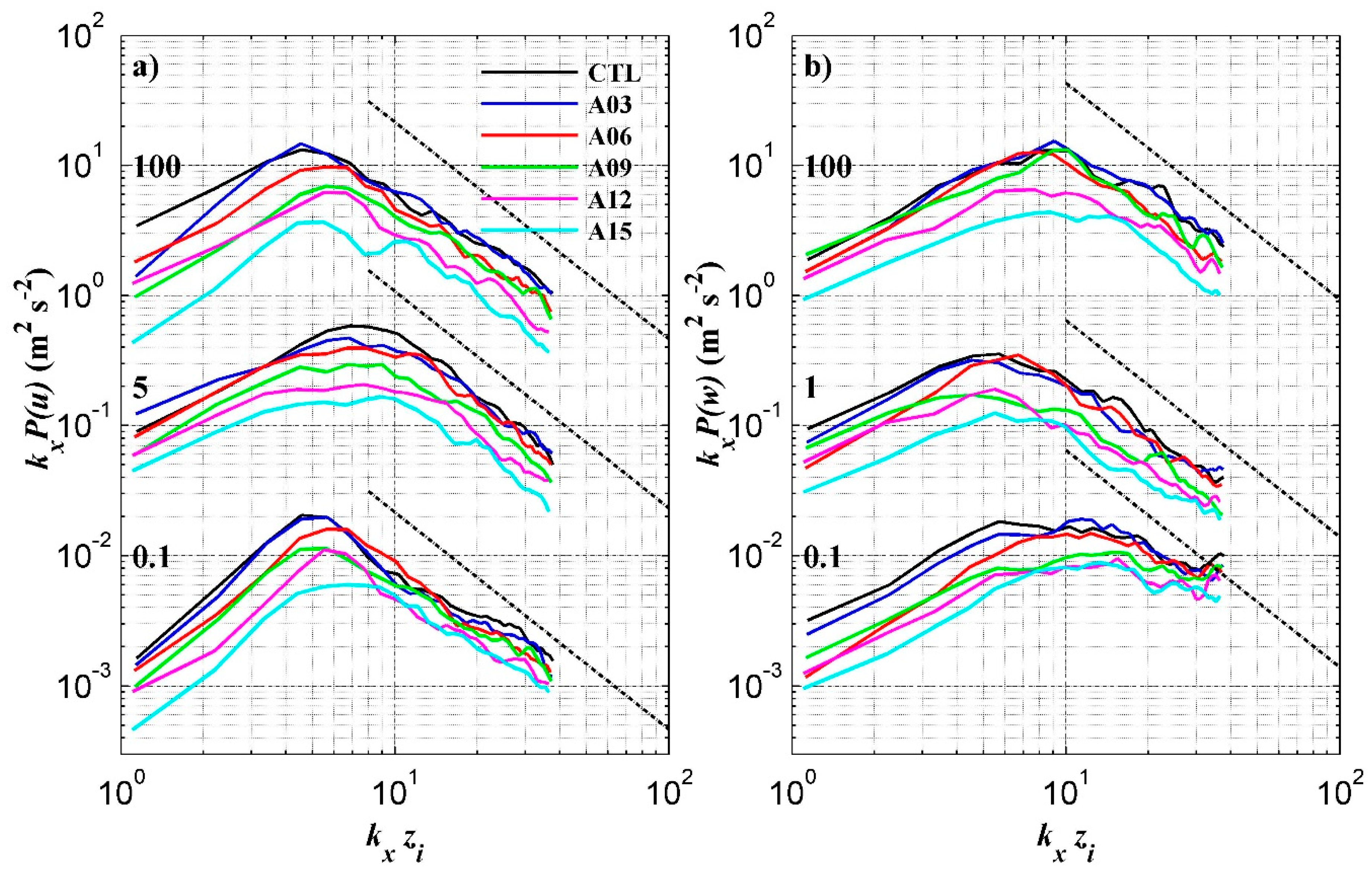
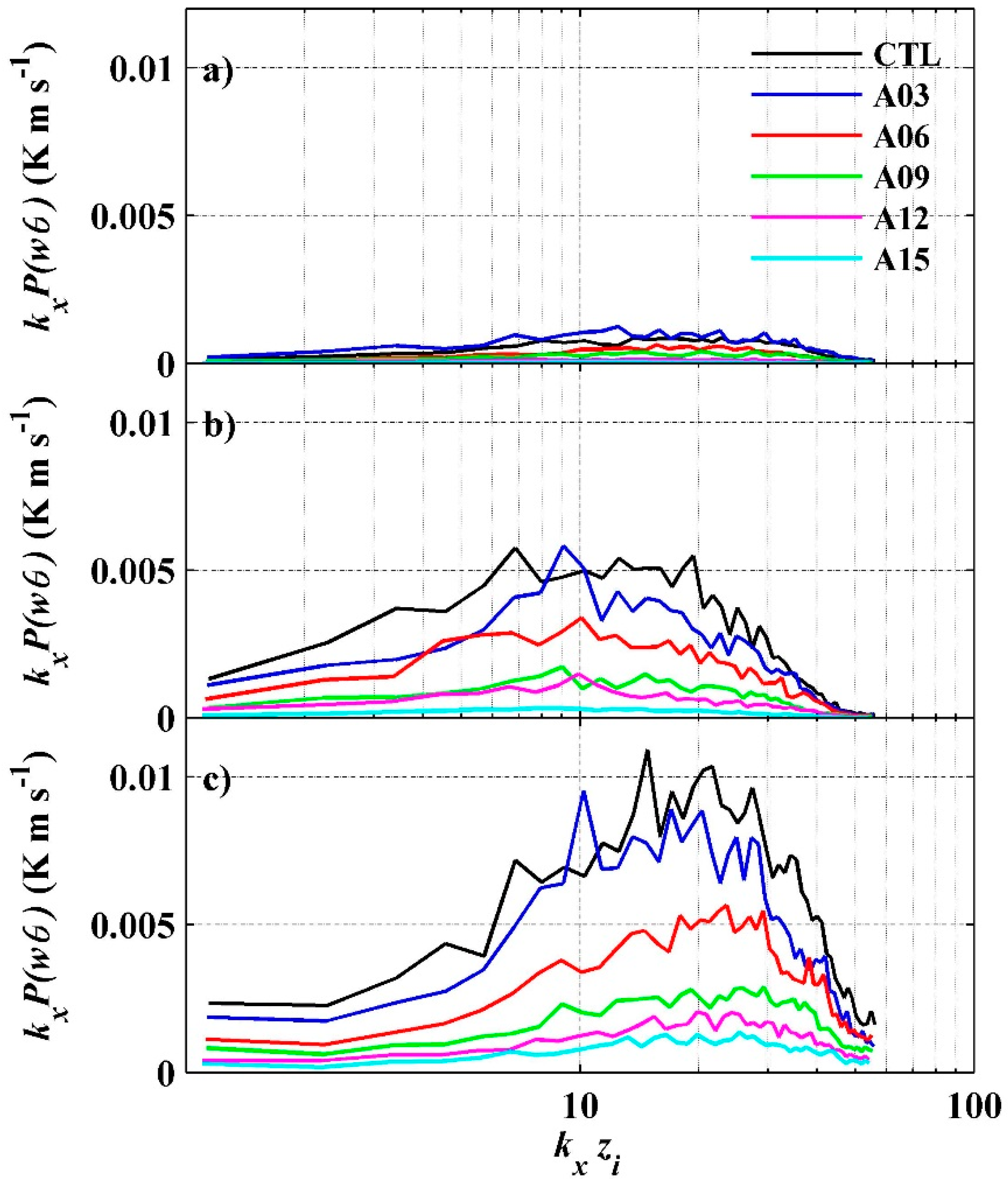
3.2. Spectral Analysis
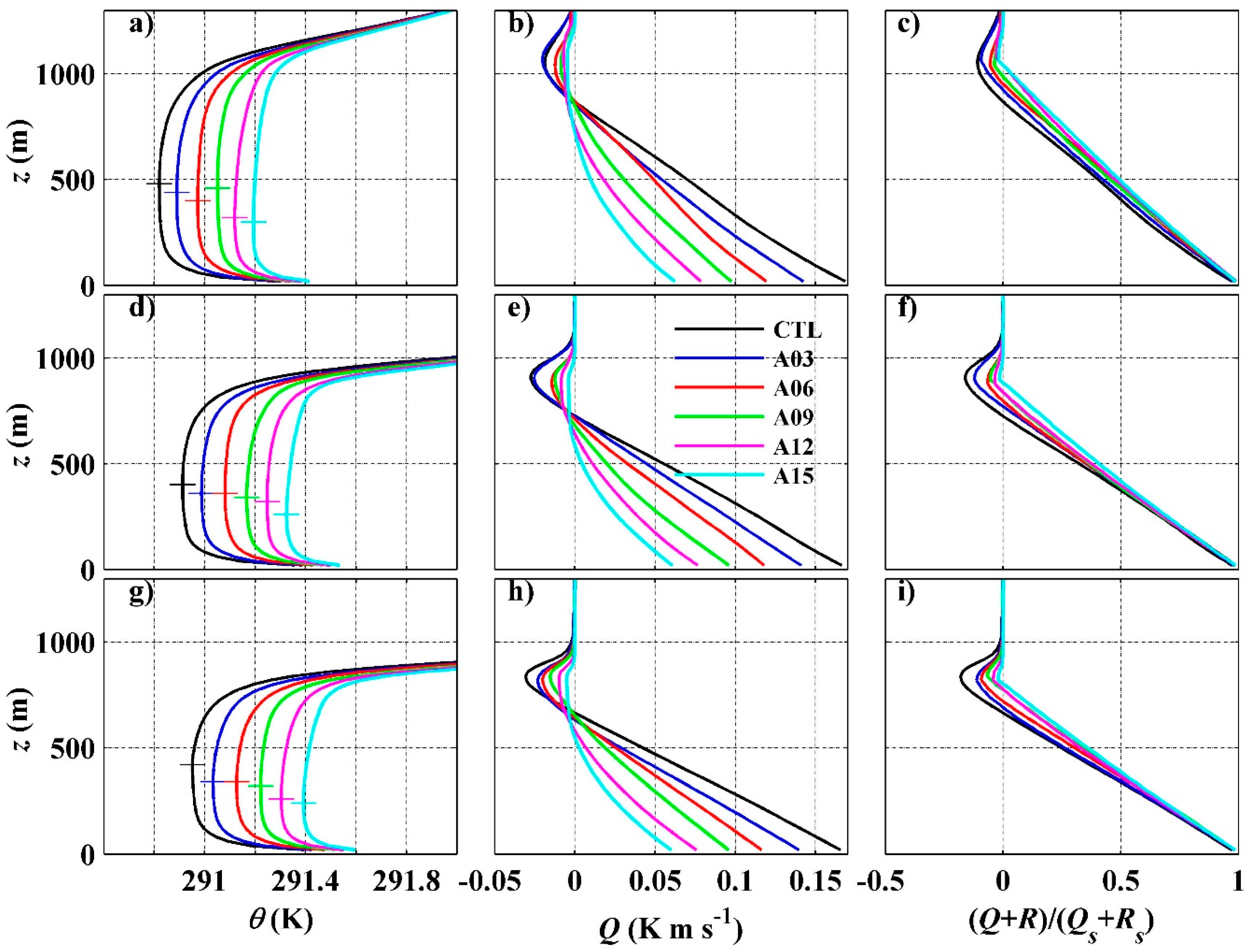
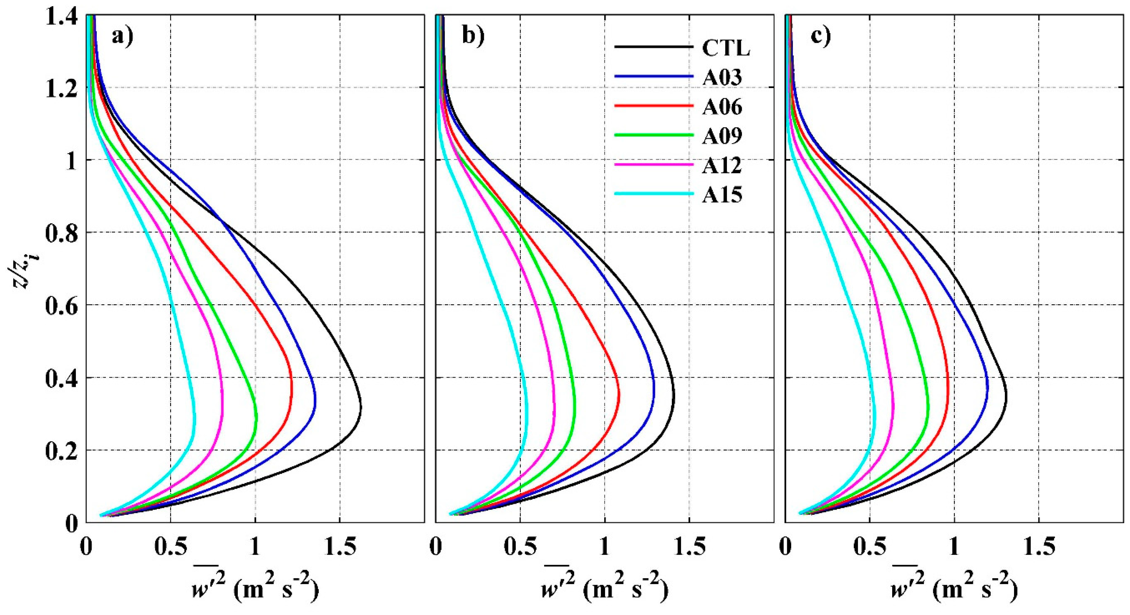
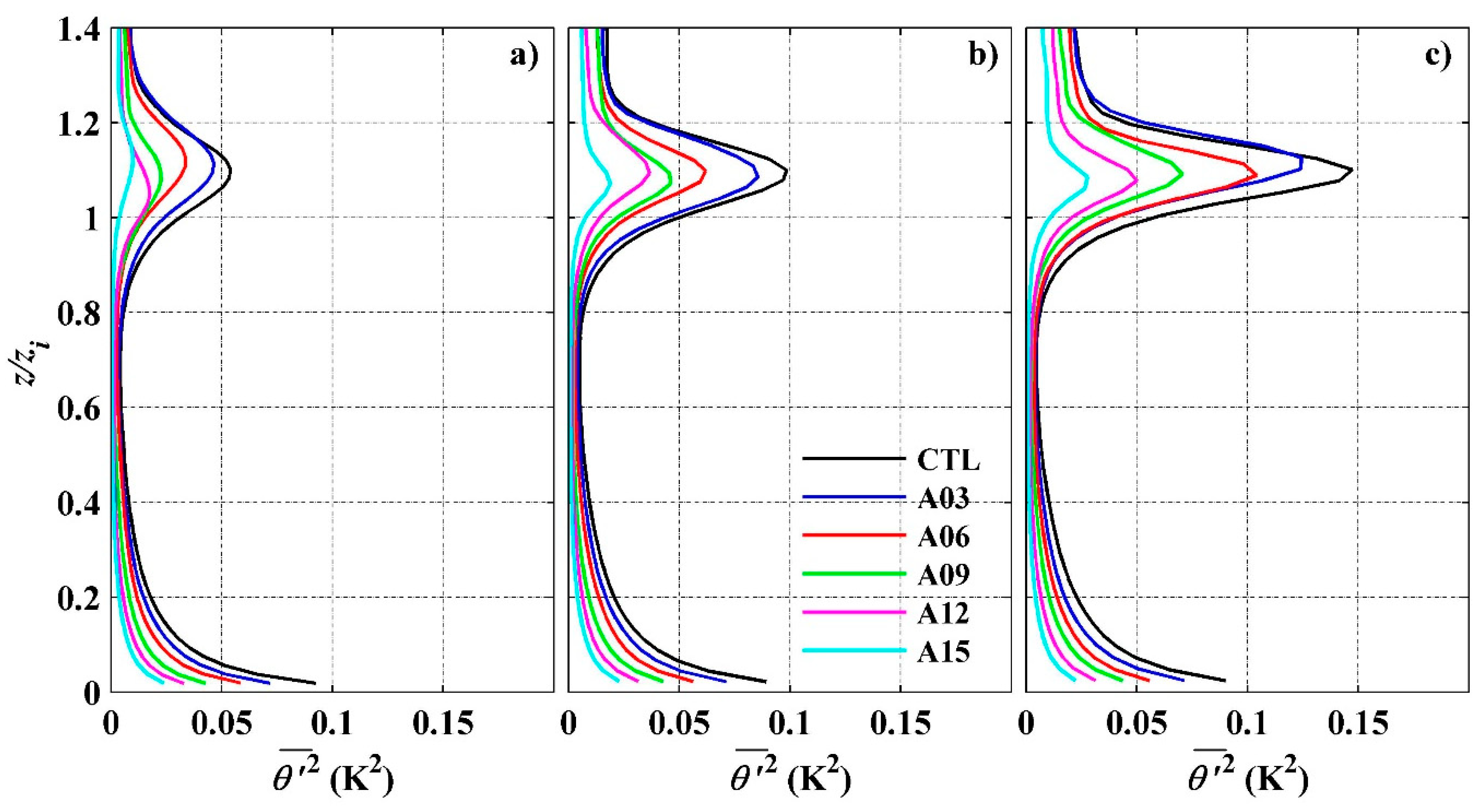
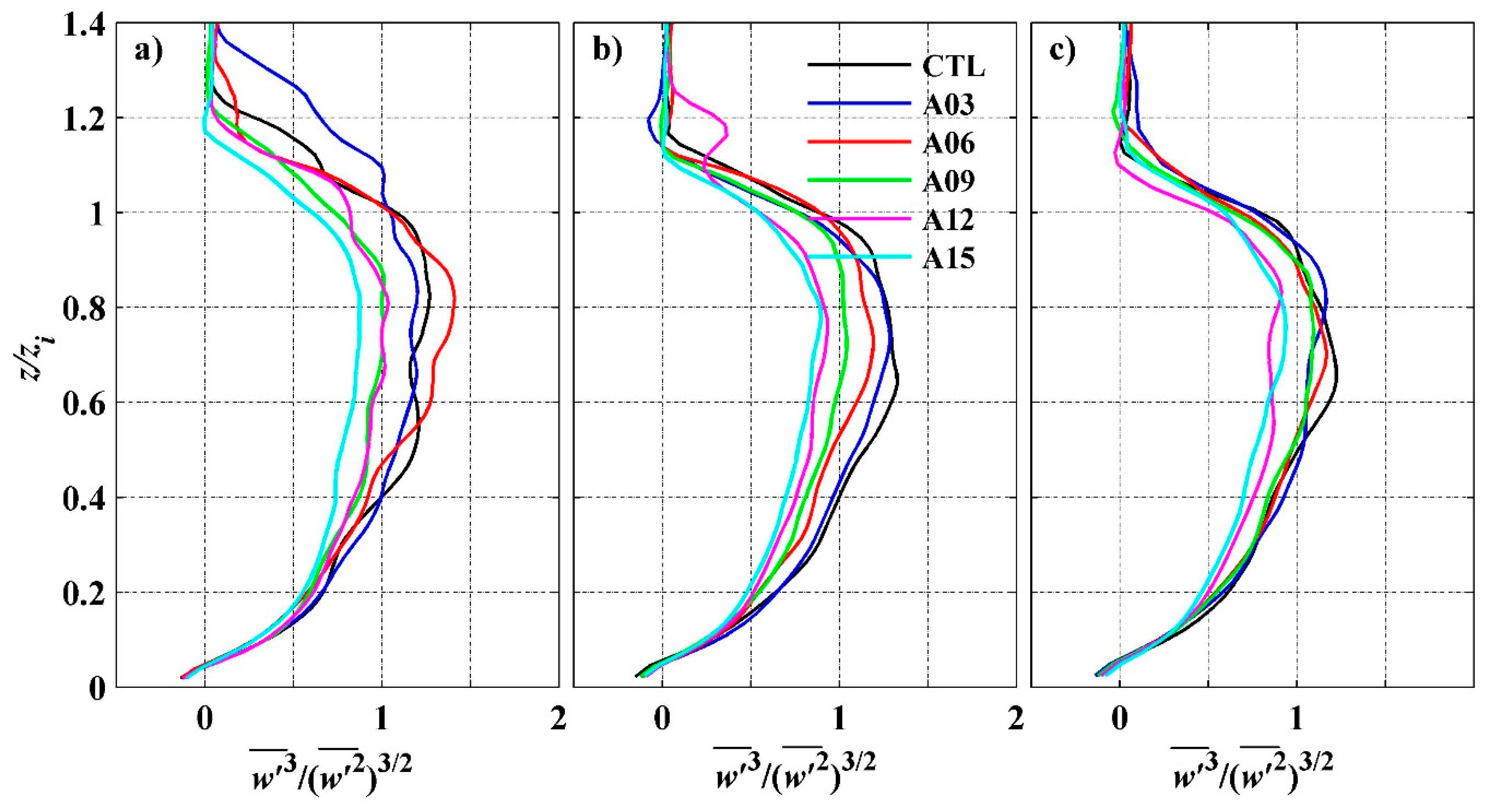
3.3. Profiles of Turbulence Statistics
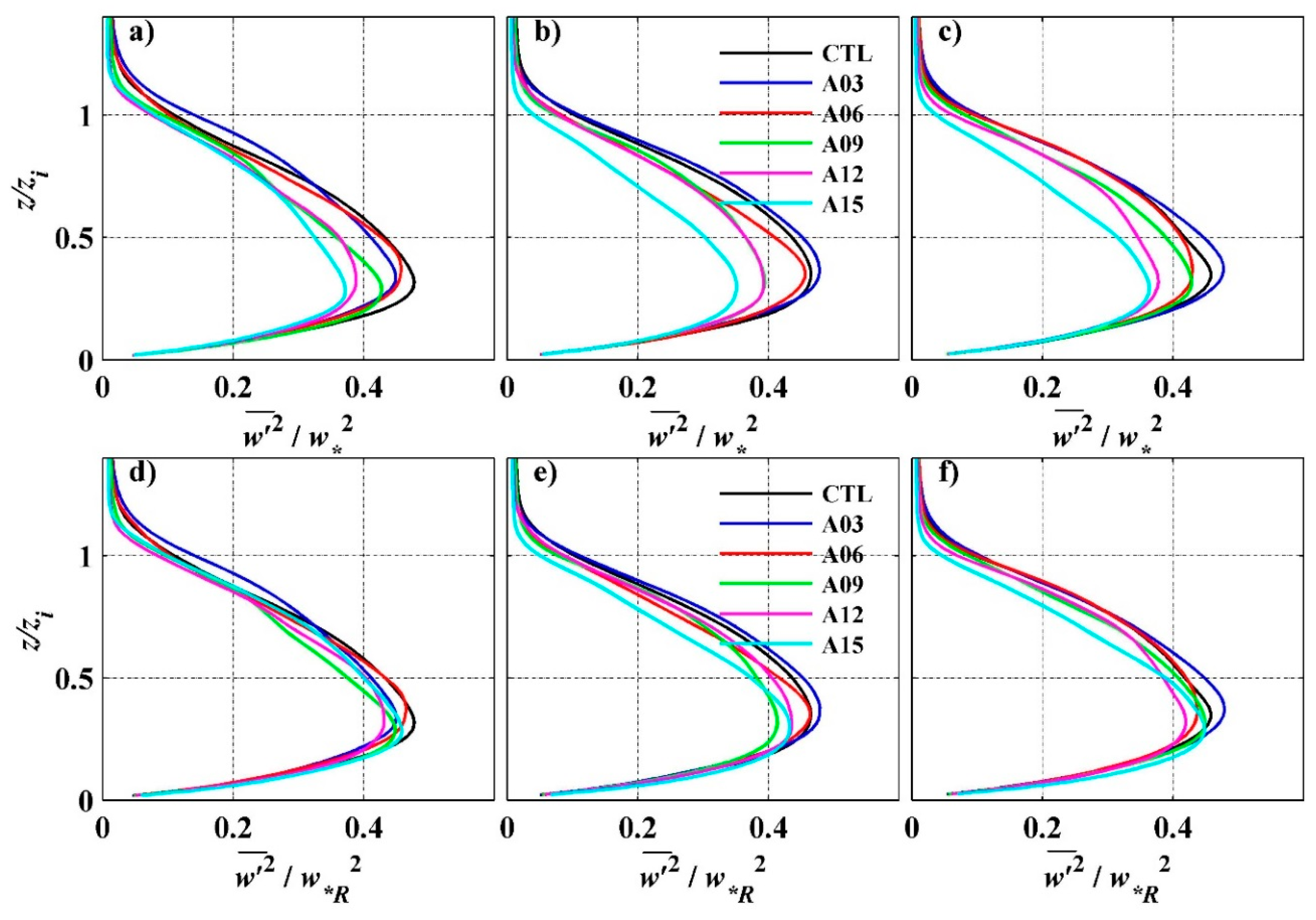
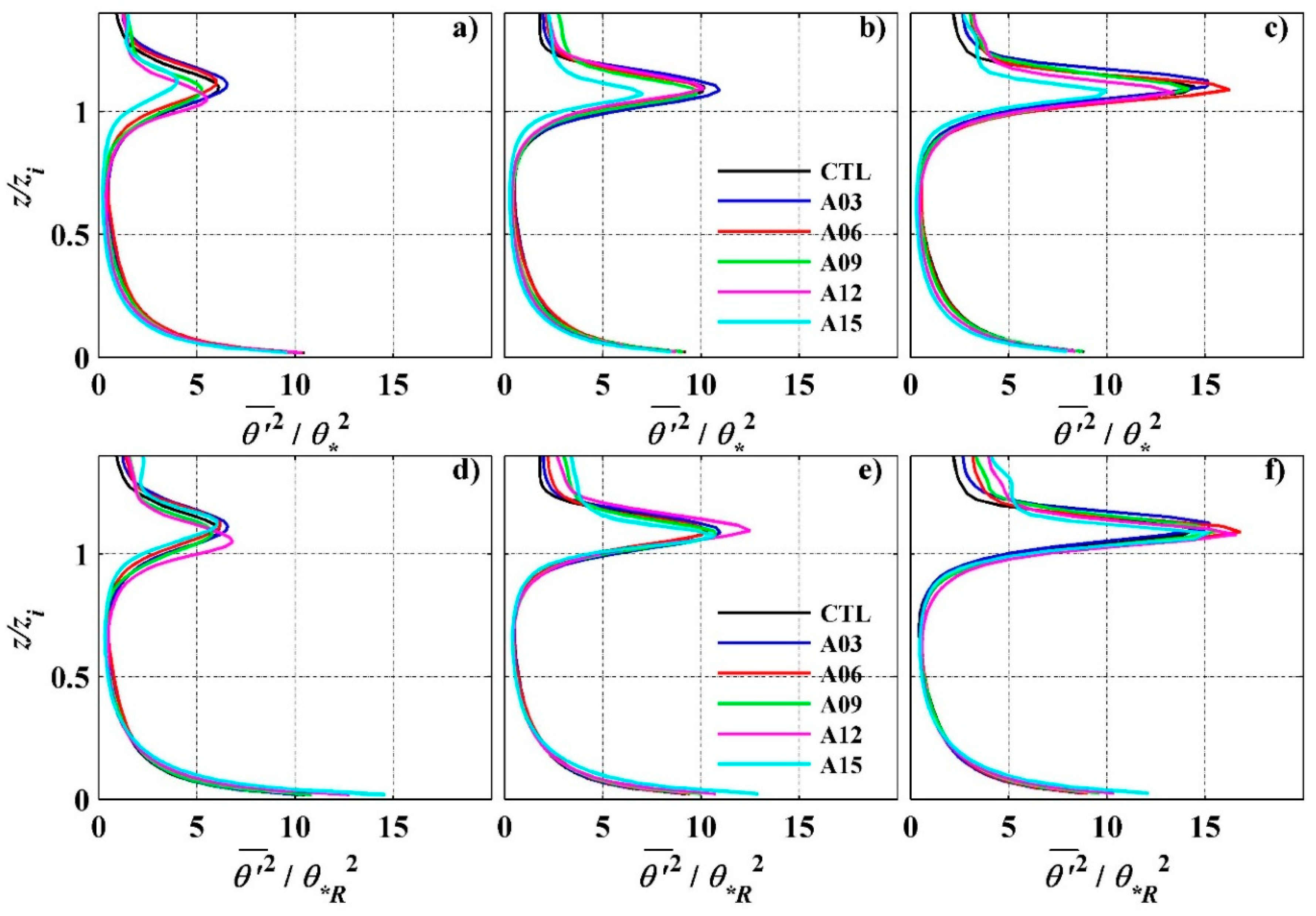
3.4. Scaling Parameters for Normalization of Statistics
4. Summary and Conclusions
Author Contributions
Funding
Acknowledgments
Conflicts of Interest
References
- Smith, F.B. Turbulence in the atmospheric boundary layer. Sci. Prog. 1975, 62, 127–151. [Google Scholar]
- Fedorovich, E.; Conzemius, R.; Mironov, D. Convective entrainment into a shear-free, linearly stratified atmosphere: Bulk models reevaluated through large eddy simulations. J. Atmos. Sci. 2004, 61, 281–295. [Google Scholar] [CrossRef]
- Liu, C.; Feorovich, E.; Huang, J. Revisiting entrainment relationships for shear-free and sheared convective boundary layers through large-eddy simulations. Q. J. R. Meteorol. Soc. 2018. [Google Scholar] [CrossRef]
- Stull, R.B. An Introduction to Boundary Layer Meteorology; Kluwer Academic Publishers: Alphen aan den Rijn, The Netherlands, 1988. [Google Scholar]
- Oboukhov, A.M. Some specific features of atmospheric tubulence. J. Fluid Mech. 1962, 13, 77–81. [Google Scholar] [CrossRef]
- Nieuwstadt, F.T.M.; Duynkerke, P.G. Turbulence in the atmospheric boundary layer. Atmos. Res. 1996, 40, 111–142. [Google Scholar] [CrossRef]
- Lee, X.; Gao, Z.; Zhang, C.; Chen, F.; Hu, Y.; Jiang, W.; Liu, S.; Lu, L.; Sun, J.; Wang, J.; et al. Priorities for boundary layer meteorology research in China. Bull. Am. Meteorol. Soc. 2015, 96, ES149–ES151. [Google Scholar] [CrossRef]
- Yu, H.; Liu, S.C.; Dickinson, R.E. Radiative effects of aerosols on the evolution of the atmospheric boundary layer. J. Geophys. Res. Atmos. 2002, 107, 4142. [Google Scholar] [CrossRef]
- Kedia, S.; Ramachandran, S.; Kumar, A.; Sarin, M.M. Spatiotemporal gradients in aerosol radiative forcing and heating rate over Bay of Bengal and Arabian Sea derived on the basis of optical, physical, and chemical properties. J. Geophys. Res. Atmos. 2010, 115, D07205. [Google Scholar] [CrossRef]
- Barbaro, E.; Vilà-Guerau de Arellano, J.; Krol, M.C.; Holtslag, A.A. Impacts of aerosol shortwave radiation absorption on the dynamics of an idealized convective atmospheric boundary layer. Bound.-Layer Meteorol. 2013, 148, 31–49. [Google Scholar] [CrossRef]
- Ding, A.J.; Huang, X.; Nie, W.; Sun, J.N.; Kerminen, V.M.; Petäjä, T.; Su, H.; Cheng, Y.F.; Wang, X.Q.; Wang, M.H.; et al. Enhanced haze pollution by black carbon in megacities in China. Geophys. Res. Lett. 2016, 43, 2873–2879. [Google Scholar] [CrossRef] [Green Version]
- Li, Z.; Guo, J.; Ding, A.; Liao, H.; Liu, J.; Sun, Y.; Wang, T.; Xue, H.; Zhang, H.; Zhu, B. Aerosol and boundary-layer interactions and impact on air quality. Natl. Sci. Rev. 2017, 4, 810–833. [Google Scholar] [CrossRef] [Green Version]
- Angevine, W.M.; Grimsdell, A.W.; McKeen, S.A.; Warnock, J.M. Entrainment results from the Flatland boundary layer experiments. J. Geophys. Res. Atmos. 1998, 103, 13689–13701. [Google Scholar] [CrossRef] [Green Version]
- Raga, G.B.; Castro, T.; Baumgardner, D. The impact of megacity pollution on local climate and implications for the regional environment: Mexico City. Atmos. Environ. 2001, 35, 1805–1811. [Google Scholar] [CrossRef]
- Gao, Y.; Zhang, M.; Liu, Z.; Wang, L.; Wang, P.; Xia, X.; Tao, M.; Zhu, L. Modeling the feedback between aerosol and meteorological variables in the atmospheric boundary layer during a severe fog-haze event over the North China Plain. Atmos. Chem. Phys. 2015, 15, 4279–4295. [Google Scholar] [CrossRef]
- Qiu, Y.; Liao, H.; Zhang, R.; Hu, J. Simulated impacts of direct radiative effects of scattering and absorbing aerosols on surface-layer aerosol concentrations in China during a heavily polluted event in February 2014. J. Geophys. Res. Atmos. 2017, 122, 5955–5975. [Google Scholar] [CrossRef]
- Ackerman, T.P. A model of the effect of aerosols on urban climates with particular applications to the Los Angeles basin. J. Atmos. Sci. 1977, 34, 531–547. [Google Scholar] [CrossRef]
- Deardorff, J.W. 1972: Numerical investigation of neutral and unstable planetary boundary layers. J. Atmos. Sci. 1972, 29, 91–115. [Google Scholar] [CrossRef]
- Moeng, C.H. A large-eddy-simulation model for the study of planetary boundary-layer turbulence. J. Atmos. Sci. 1984, 41, 2052–2062. [Google Scholar] [CrossRef]
- Sullivan, P.P.; McWilliams, J.C.; Moeng, C.H. A grid nesting method for large-eddy simulation of planetary boundary-layer flows. Bound.-Layer Meteorol. 1996, 80, 167–202. [Google Scholar] [CrossRef]
- Huang, J.; Lee, X.; Patton, E.G. Dissimilarity of scalar transport in the convective boundary layer in inhomogeneous landscapes. Bound.-Layer Meteorol. 2009, 130, 327–345. [Google Scholar] [CrossRef]
- Huang, J.; Lee, X.; Patton, E.G. Entrainment and budgets of heat, water vapor, and carbon dioxide in a convective boundary layer driven by time-varying forcing. J. Geophys. Res. Atmos. 2011, 116, D06308. [Google Scholar] [CrossRef]
- Archer-Nicholls, S.; Lowe, D.; Schultz, D.M.; McFiggans, G. Aerosol–radiation–cloud interactions in a regional coupled model: The effects of convective parameterization and resolution. Atmos. Chem. Phys. 2016, 16, 5573–5594. [Google Scholar] [CrossRef]
- Kaimal, J.C.; Wyngaard, J.C.; Haugen, D.A.; Coté, O.R.; Izumi, Y.; Caughey, S.J.; Readings, C.J. Turbulence structure in the convective boundary layer. J. Atmos. Sci. 1976, 33, 2152–2169. [Google Scholar] [CrossRef]
- Huang, J.; Lee, X.; Patton, E.G. A modelling study of flux imbalance and the influence of entrainment in the convective boundary layer. Bound.-Layer Meteorol. 2008, 127, 273–292. [Google Scholar] [CrossRef]
- Sullivan, P.P.; Moeng, C.H.; Stevens, B.; Lenschow, D.H.; Mayor, S.D. Structure of the entrainment zone capping the convective atmospheric boundary layer. J. Atmos. Sci. 1998, 55, 3042–3064. [Google Scholar] [CrossRef]
- Moeng, C.H.; Sullivan, P.P.; Stevens, B. Including radiative effects in an entrainment rate formula for buoyancy-driven PBLs. J. Atmos. Sci. 1999, 56, 1031–1049. [Google Scholar] [CrossRef]
- Moeng, C.H.; Rotunno, R. Vertical-velocity skewness in the buoyancy-driven boundary layer. J. Atmos. Sci. 1990, 47, 1149–1162. [Google Scholar] [CrossRef]
- Hogan, R.J.; Grant, A.L.; Illingworth, A.J.; Pearson, G.N.; O’Connor, E.J. Vertical velocity variance and skewness in clear and cloud-topped boundary layers as revealed by Doppler lidar. Q. J. R. Meteorol. Soc. 2009, 135, 635–643. [Google Scholar] [CrossRef]
- Deardorff, J.W. Convective velocity and temperature scales for the unstable planetary boundary layer and for Rayleigh convection. J. Atmos. Sci. 1970, 27, 1211–1213. [Google Scholar] [CrossRef]
- Lee, X. Turbulence spectra and eddy diffusivity over forests. J. Appl. Meteo. 1996, 35, 1307–1318. [Google Scholar] [CrossRef]
- Kaimal, J.C.; Wyngaard, J.C.; Izumi, Y.; Coté, O.R. Spectral characteristics of surface-layer turbulence. Q. J. R. Meteorol. Soc. 1972, 98, 563–589. [Google Scholar] [CrossRef] [Green Version]
- Moraes, O.L.; Fitzjarrald, D.R.; Acevedo, O.C.; Sakai, R.K.; Czikowsky, M.J.; Degrazia, G.A. Comparing spectra and cospectra of turbulence over different surface boundary conditions. Phys. A Stat. Mech. Appl. 2008, 387, 4927–4939. [Google Scholar] [CrossRef]
- Moeng, C.H.; Wyngaard, J.C. Spectral analysis of large-eddy simulations of the convective boundary layer. J. Atmos. Sci. 1988, 45, 3573–3587. [Google Scholar] [CrossRef]
- Schmidt, H.; Schumann, U. Coherent structure of the convective boundary layer derived from large-eddy simulations. J. Fluid Mech. 1989, 200, 511–562. [Google Scholar] [CrossRef]
- Sullivan, P.P.; Patton, E.G. The effect of mesh resolution on convective boundary layer statistics and structures generated by large-eddy simulation. J. Atmos. Sci. 2011, 68, 2395–2415. [Google Scholar] [CrossRef]
- Gibbs, J.A.; Fedorovich, E. Effects of temporal discretization on turbulence statistics and spectra in numerically simulated convective boundary layers. Bound.-Layer Meteorol. 2014, 153, 19–41. [Google Scholar] [CrossRef]
- Gibbs, J.A.; Fedorovich, E. Comparison of convective boundary layer velocity spectra retrieved from large-eddy-simulation and weather research and forecasting model data. J. Appl. Meteorol. Climatol. 2014, 53, 377–394. [Google Scholar] [CrossRef]
- Liu, C.; Fedorovich, E.; Huang, J.; Hu, X.M.; Wang, Y.; Lee, X. Impact of aerosol shortwave radiative heating on the entrainment in atmospheric convective boundary layer: A large-eddy simulation study. J. Atmos. Sci. 2018. in revision. [Google Scholar]
- Patton, E.G.; Sullivan, P.P.; Moeng, C.H. The influence of idealized heterogeneity on wet and dry planetary boundary layers coupled to the land surface. J. Atmos. Sci. 2005, 62, 2078–2097. [Google Scholar] [CrossRef]
- Ricchiazzi, P.; Yang, S.; Gautier, C.; Sowle, D. SBDART: A research and teaching software tool for plane-parallel radiative transfer in the Earth’s atmosphere. Bull. Amer. Meteor. Soc. 1998, 79, 2101–2114. [Google Scholar] [CrossRef]
- Steyn, D.G.; Baldi, M.; Hoff, R.M. The detection of mixed layer depth and entrainment zone thickness from lidar backscatter profiles. J. Atmos. Ocean Technol. 1999, 16, 953–959. [Google Scholar] [CrossRef]
- Ferrero, L.; Riccio, A.; Perrone, M.G.; Sangiorgi, G.; Ferrini, B.S.; Bolzacchini, E. Mixing height determination by tethered balloon-based particle soundings and modeling simulations. Atmos. Res. 2011, 102, 145–156. [Google Scholar] [CrossRef]
- Ware, J.; Kort, E.A.; DeCola, P.; Duren, R. Aerosol lidar observations of atmospheric mixing in Los Angeles: Climatology and implications for greenhouse gas observations. J. Geophys. Res. Atmos. 2016, 121, 9862–9878. [Google Scholar] [CrossRef] [PubMed] [Green Version]
- Liou, K.N. An Introduction to Atmospheric Radiation; Academic Press: New York, NY, USA, 2002. [Google Scholar]
- Kleeman, M.J.; Cass, G.R.; Eldering, A. Modeling the airborne particle complex as a source- oriented external mixture. J. Geophys. Res. Atmos. 1997, 102, 21355–21372. [Google Scholar] [CrossRef]
- Riemer, N.; Vogel, H.; Vogel, B.; Fiedler, F. Modeling aerosols on the mesoscale-γ: Treatment of soot aerosol and its radiative effects. J. Geophys. Res. Atmos. 2003, 108. [Google Scholar] [CrossRef] [Green Version]
- Pino, D.; Vilà-Guerau De Arellano, J. Effects of shear in the convective boundary layer: Analysis of the turbulent kinetic energy budget. Acta Geophys. 2008, 56, 167–193. [Google Scholar] [CrossRef]
- Kaufman, Y.J. Aerosol optical thickness and atmospheric path radiance. J. Geophys. Res. Atmos. 1993, 98, 2677–2692. [Google Scholar] [CrossRef] [Green Version]
- Tao, M.; Chen, L.; Xiong, X.; Zhang, M.; Ma, P.; Tao, J.; Wang, Z. Formation process of the widespread extreme haze pollution over northern China in January 2013: Implications for regional air quality and climate. Atmos. Environ. 2014, 98, 417–425. [Google Scholar] [CrossRef]
- Liu, J.; Zheng, Y.; Li, Z.; Flynn, C.; Cribb, M. Seasonal variations of aerosol optical properties, vertical distribution and associated radiative effects in the Yangtze Delta region of China. J. Geophys. Res. Atmos. 2012, 117. [Google Scholar] [CrossRef] [Green Version]
- Klemp, J.B.; Durran, D.R. An upper boundary condition permitting internal gravity wave radiation in numerical mesoscale models. Mon. Weather Rev. 1983, 111, 430–444. [Google Scholar] [CrossRef]
- Kanda, M.; Inagaki, A.; Letzel, M.O.; Raasch, S.; Watanabe, T. LES study of the energy imbalance problem with eddy covariance fluxes. Bound.-Layer Meteorol. 2004, 110, 381–404. [Google Scholar] [CrossRef]
- Su, H.B.; Paw U, K.T.; Shaw, R.H. Development of a coupled leaf and canopy model for the simulation of plant-atmosphere interaction. J. Appl. Meteorol. 1996, 35, 733–748. [Google Scholar] [CrossRef]
- Kaiser, R.; Fedorovich, E. Turbulence spectra and dissipation rates in a wind tunnel model of the atmospheric convective boundary layer. J. Atmos. Sci. 1998, 55, 580–594. [Google Scholar] [CrossRef]
- Barbaro, E.W. Interactions between Aerosal and Convective Boundary-Layer Dynamics over Land; Wageningen University: Wageningen, The Netherlands, 2015. [Google Scholar]
- Sorbjan, Z. Effects caused by varying the strength of the capping inversion based on a large eddy simulation model of the shear-free convective boundary layer. J. Atmos. Sci. 1996, 53, 2015–2024. [Google Scholar] [CrossRef]


| Characteristic | Setting |
|---|---|
| Domain size | 5 km × 5 km × 1.92 km |
| Grid spacing | 50 m × 50 m × 20 m |
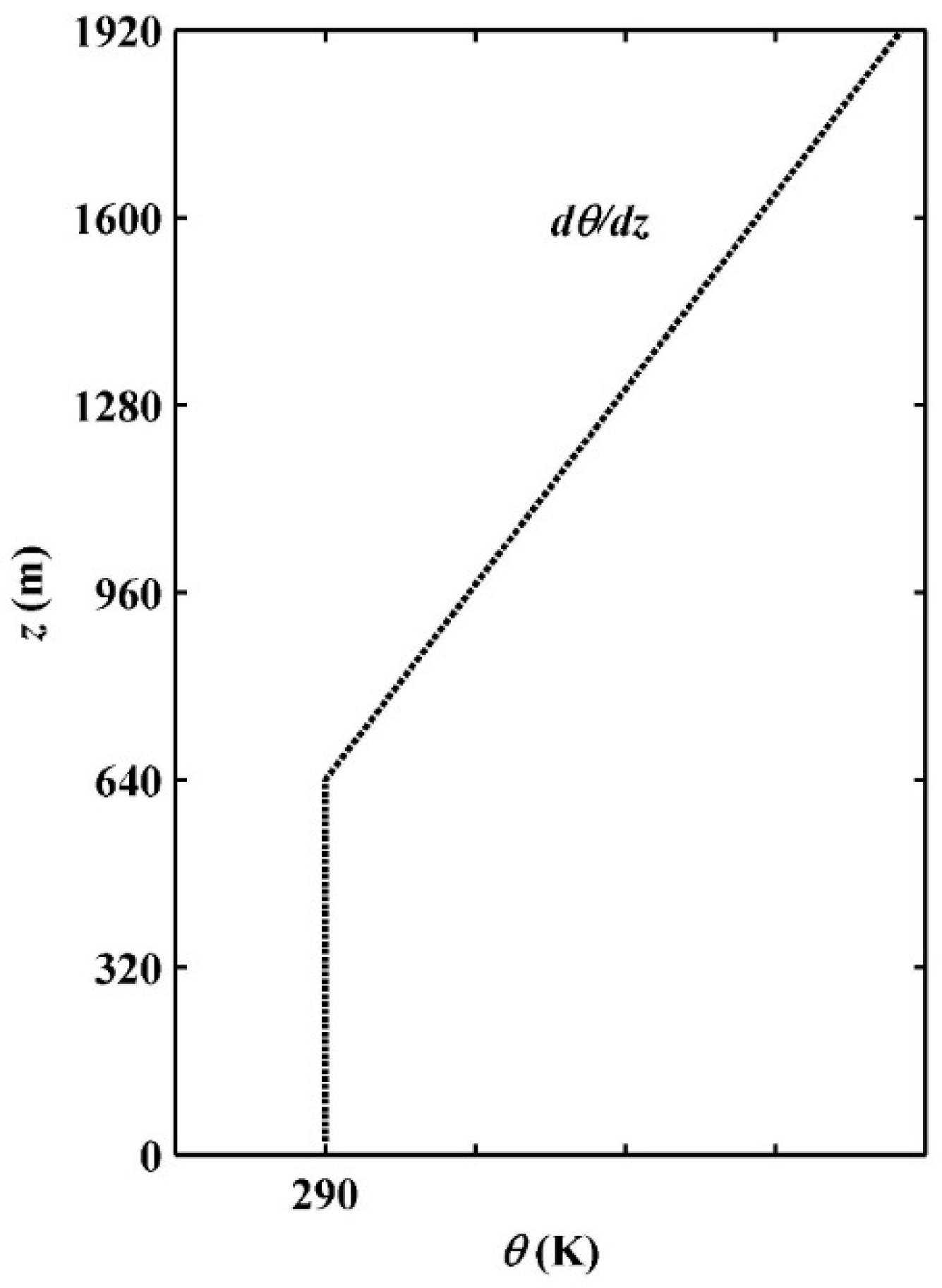
| Temperature gradient above CBL | dθ/dz = 3 K km−1, 6 K km−1, and 9 K km−1 |
| Time step | Determined from a numerical stability constraint, varies from 1.6 s to 2.0 s |
| Lateral boundary layer conditions | Periodic |
| Upper boundary layer conditions | A radiation boundary layer condition [52] |
| Lower boundary layer conditions | No slip for velocity and Monin-Obukhov similarity |
| Aerosol optical depth (AOD) | CTL: 0, A03: 0.3, A06: 0.6, A09: 0.9, A12: 1.2, A15: 1.5 |
| Single scattering albedo (SSA) | 0.9 |
| Asymmetry factor (gf) | 0.6 |
© 2018 by the authors. Licensee MDPI, Basel, Switzerland. This article is an open access article distributed under the terms and conditions of the Creative Commons Attribution (CC BY) license (http://creativecommons.org/licenses/by/4.0/).
Share and Cite
Liu, C.; Huang, J.; Fedorovich, E.; Hu, X.-M.; Wang, Y.; Lee, X. The Effect of Aerosol Radiative Heating on Turbulence Statistics and Spectra in the Atmospheric Convective Boundary Layer: A Large-Eddy Simulation Study. Atmosphere 2018, 9, 347. https://doi.org/10.3390/atmos9090347
Liu C, Huang J, Fedorovich E, Hu X-M, Wang Y, Lee X. The Effect of Aerosol Radiative Heating on Turbulence Statistics and Spectra in the Atmospheric Convective Boundary Layer: A Large-Eddy Simulation Study. Atmosphere. 2018; 9(9):347. https://doi.org/10.3390/atmos9090347
Chicago/Turabian StyleLiu, Cheng, Jianping Huang, Evgeni Fedorovich, Xiao-Ming Hu, Yongwei Wang, and Xuhui Lee. 2018. "The Effect of Aerosol Radiative Heating on Turbulence Statistics and Spectra in the Atmospheric Convective Boundary Layer: A Large-Eddy Simulation Study" Atmosphere 9, no. 9: 347. https://doi.org/10.3390/atmos9090347