Article

Effects of El-Niño, Indian Ocean Dipole, and Madden-Julian Oscillation on Surface Air Temperature and Rainfall Anomalies over Southeast Asia in 2015

1
Department of Civil Engineering, Faculty of Engineering, University of Nottingham, Malaysia Campus, Jalan Broga, Semenyih 43500, Selangor, Malaysia
2
School of Environmental and Geographical Sciences, Faculty of Science, University of Nottingham, Malaysia Campus, Jalan Broga, Semenyih 43500, Selangor, Malaysia
3
Department of Atmospheric Sciences, National Central University, Chung-Li 32001, Taiwan
*
Authors to whom correspondence should be addressed.
Atmosphere 2018, 9(9), 352; https://doi.org/10.3390/atmos9090352
Submission received: 16 June 2018 / Revised: 3 September 2018 / Accepted: 3 September 2018 / Published: 12 September 2018
(This article belongs to the Special Issue Monsoons)

Abstract

:
The Maritime Continent (MC) is positioned between the Asian and Australian summer monsoons zone. The complex topography and shallow seas around it are major challenges for the climate researchers to model and understand it. It is also the centre of the tropical warm pool of Southeast Asia (SEA) and therefore the MC gets extra attention of the researchers. The monsoon in this area is affected by inter-scale ocean-atmospheric interactions such as the El-Niño Southern Oscillation (ENSO), the Indian Ocean Dipole (IOD), and the Madden-Julian Oscillation (MJO). Monsoon rainfall in the MC (especially in Indonesia and Malaysia) profoundly exhibits its variability dependence on ocean-atmospheric phenomena in this region. This monsoon shift often introduces to dreadful events like biomass burning (BB) in Southeast Asia (SEA) in which some led to severe trans-boundary haze pollution events in the past. In this study, the BB episode of 2015 in the MC is highlighted and discussed. Observational satellite datasets are tested by performing simulations with the numerical weather prediction (NWP) model WRF-ARW (Weather Research and Forecast—Advanced research WRF). Observed and model datasets are compared to study the surface air temperature and precipitation (rainfall) anomalies influenced by ENSO, IOD, and MJO. Links amongst these influences have been recognised and the delayed precipitation of the regular monsoon in the MC due to their influence during the 2015 BB episode is explained and accounted for, which eventually led to the intensification of fire and a severe haze.

1. Introduction

In climate research, the maritime continent (MC) is one of the most crucial regions [1]. The MC plays a key role as a heat and moisture source and impacts global atmospheric circulations that contribute to regional climate change [2]. The MC is known to be a very active convective region where convection is influenced by local, regional, and global atmospheric conditions such as the monsoon, tropical convection, intra-seasonal oscillations, and the complex structure of the topography of land and the body of water around it [3,4]. The intertropical convergence zone (ITCZ) and its effects on surface air temperature and active precipitation are vital for convection in the MC region [5]. Despite its importance, the inter-scale interactions of intra-seasonal and mesoscale variability forced by diurnal affects (e.g., oceanic circulation, wind, temperature, and precipitation) errors are often found in the climate models of the MC [6]. The MC also has a signature seasonal cycle of its rainfall that characterises a typical monsoon climate [7]. Due to the complex topography of the region and vast unpopulated land areas, the dense rain gauge network is absent in most places of the MC and gauge observation in the oceanic areas are not possible to obtain [8]. Satellite observation is the best available solution in such cases to attain adequate temporal and spatial coverage of rainfall data [9]. Therefore, in this study, a computer model is used where the observational satellite data are used as feed to investigate surface air temperature and precipitation (rainfall).
In the atmosphere around the MC, the most important source of pollution is fire, which comes in forms of aerosol particles, greenhouse gases, or different trace gases [10]. Not only the air quality depends on fire but also the whole ecosystem, public health, land use, and safety. Improvements of satellite data provide much better observational skills in our time to study weather and the climate more comprehensively [11]. Global emission inventories are being checked regularly near real time to achieve most accurate data. The spatial resolution of satellite imageries has been improved, which now helps to obtain data on an hourly basis [12].
Biomass Burning (BB) in the MC is a regular event and engenders air pollution on a very large scale (when air particles propagate as haze) with immense impacts on economics and public health of the region [13]. BB events usually occur in dry seasons and vary in degrees. Since 1972, almost all hazes in the Southeast Asia (SEA) region have been recorded as trans-boundary [14]. The slash-and-burn practice mostly in Indonesia and illegal extension of agricultural lands are the main anthropogenic reasons of BB in the MC region. Historically, it starts from Southern Sumatra and Kalimantan on the Indonesian part of Borneo [15]. In the early 2000s, after the Earth Observing Satellite System by the National Aeronautics and Space Administration (NASA) started its observations, it has been shown that BB of 2015 and its haze episode in SEA was the most severe in terms of fire activity and pollution. The CO2 equivalent emission during this period alone stood for 2013 annual CO2 emissions of Japan and India combined [16]. Dry conditions are mainly responsible for such events and they have direct impacts on weather, climate, and public health [17]. In recent years, the MC has experienced multiple numbers of major trans-boundary haze episodes (from 1982 until 2015). Ground observation stations, satellites, and records of the airport visibility system in Sumatra and Kalimantan region (Indonesia) demonstrated that, after 1994 and 1997 BB episodes, the 2015 episode ranked among the worst on record [17]. The increasing numbers of BB episodes in the MC region cause extra economic damages. BB and the evolved haze propagate across national boundaries and contribute to the climate change not only in the MC but in the whole SEA.
Haze episodes in MC initially start because of peatland fires in Indonesia and appeared to be influenced greatly by several major ocean-atmosphere events e.g., El-Niño Southern Oscillation (ENSO), the Indian Ocean Dipole (IOD), and the Madden-Julian Oscillation (MJO). In last 30 to 40 years, 1982, 1997 and 2015 were the most severe BB haze episodes SEA has seen. They were all El-Niño and positive IOD years [18,19]. A very important climatic element of the MC is its variations in rainfall [20,21]. Over Indonesia, the variability in rainfall is strongly related to ENSO and the rainfall is anomalously low during the warm period when El-Niño is present [22]. This relationship is usually stronger during drier and transition seasons. IOD is responsible for rainfall anomalies in the MC region. ENSO and IOD caused rainfall variabilities are very unique in the Indonesian region. A strong influence is observed during drier season (June–November), but during the wet season (December–May) the influence is observed weaker [23]. Intra-seasonal variability in the MC is caused by another important ocean-atmosphere phenomenon—MJO. It is associated with enhanced or suppressed convection along with cloudiness, which, with a period of 30 to 90 days on average, propagates from the Indian Ocean towards the Pacific Ocean [23]. Although MJO is usually observed to be weakening when it reaches the MC, it is also observed sometimes when MJO initiates in the Indian Ocean but does not propagate through the MC [24]. The Asian-Australian monsoon covers the MC and the northern part of Australia and creates an annual dry and wet season [24]. MJO that passes through this region is associated with either high or low precipitation than average [25].
Transboundary haze episodes of Malaysia and Indonesia introduce the local climate to catastrophic air pollution events, which contribute to the climate variability of the SEA region. However, the rational sequences of such behavior are yet unclear since the reasons of these BB events are not well understood by any established theories and not quantified properly by any specific measured data. Therefore, it is important to establish logical sequences, physically and prognostically, to understand why and how this is happening. It will help us to learn how to take necessary steps earlier to avoid and combat these events. The BB episode of 2015 earned its global attention due to its large coverage and trans-boundary haze propagation. However, it is not well studied by climate experts so far.
This study is focused especially on the 2015 BB episode of SEA. It aims to investigate the possibilities of interactional influences of ocean-atmosphere events (ENSO, IOD, and MJO) on the intensification of the episode. We attempt to find the connections of the monsoon with seasonal and intra-seasonal oscillations. The ENSO and IOD correlations with their single and concurrent effects and MJO effects on precipitation (rainfall) are investigated and the outcomes are discussed.

2. Data and Methods

2.1. Data Source Acquisition

Irregular periodic variation in the sea surface temperature (SST) over the tropical eastern Pacific Ocean that affects the climate of tropics and subtropics is understood as ENSO. The Multivariate ENSO Index (MEI) is a parameter used to measure and characterise the intensity of ENSO in different months of the year. For monitoring ENSO on a regular basis, the most comprehensive index is MEI since it combines the analysis of both meteorological and oceanic components [26]. MEI is determined by an International Comprehensive Ocean-Atmosphere Data Set (ICOADS). MEI datasets are used in this study and collected from the regularly updated archive of the Earth System Research Laboratory (ESRL) of National Oceanic and Atmospheric Administration (NOAA) [27].
Another irregular oscillation of SST arises from the western Indian Ocean, which becomes alternately warmer and then colder than the eastern part of the ocean. This effect is measured by the IOD. The intensity of IOD is represented by the Dipole Mode Index (DMI), which shows the SST gradient between the western equatorial Indian Ocean (50° E–70° E and 10° S–10° N) and the south eastern equatorial Indian Ocean (90° E–110° E and 10° S–0°) [28]. DMI datasets are used in this study and collected from the Global Climate Observing System (GCOS) datasets archive, which is a funded programme under the World Meteorological Organisation (WMO) [29].
An index, called the Real-time Multivariate MJO that is seasonally independent to describe and monitor MJO has been devised [30]. The index is based on a pair of empirical orthogonal functions (EOFs) that give an effective series to monitor MJO in real time series (namely RMM1 and RMM2). MJO phase progressions are generally illustrated by a phase diagram. RMM1 and RMM2 are mathematical methods that combine the cloud amount and winds, which provide a measure of MJO intensity in real time and location of its existence in the phase diagram. MJO indices move anti-clockwise from west to east. When the index is located inside the circle (phase diagram) at the center, MJO is considered the weakest. As far it goes out of the circle the MJO becomes stronger. This MJO phase diagram contains eight different phases to identify its location and progression in real time with the least amount of errors. The Bureau of Meteorology, Australia (BoM) regularly measures and updates MJO phases, their intensity, and location [31]. Outgoing longwave radiation (OLR) is also considered for this study, which is the electromagnetic radiation emitted from Earth and its atmosphere in the form of thermal radiation and measured in W/m2 [32]. OLR shows a map associated with cloudiness (below normal, normal, and above normal) and is used for the identification of cloudiness over a specific region. The BoM regularly updates the OLR maps too and data for the study are collected from their archive [33].
Satellite datasets [34] show that all the year-round biomass is continuously burning (more or less) either because of natural or anthropogenic reasons. However, BB in the MC expands uncontrollably during the drier season (June–November). Adequate rainfall is usually capable of mitigating regular BB events to prevent them from becoming disastrous as it was during the 2015 BB episode in SEA. For this study, we collect and study monthly rainfall analysis data of MC (July–December 2015) [35].
The Weather Research and Forecast (WRF) is a numerical weather prediction (NWP) system that is designed for simulating satellite data and forecast the atmosphere by computer models. WRF-ARW (Advanced Research WRF) version 3.7 is used as a weather simulation tool for this study. It contains different ranges of meteorological applications where the scales range from meters to thousands of kilometers. Global Data Assimilation Systems (GDAS) continuously gathers observational data from the Global Telecommunications System (GTS) and other verified sources. The GDAS product used for this study is the “NCEP/GDAS FNL 0.25-degree Global Tropospheric Analyses and Forecast Grids” [36].

2.2. Methodology

In this study, we investigate the BB episode of 2015 in SEA, which is a well-known El-Niño year [37]. To examine the significance of 2015, MEI values of five consecutive years (2013–2017) have been observed and compared.
Positive values of DMI indicate positive IOD and negative values indicate negative IOD. Similarly, concerning MEI, five years of data (2013–2017) have been observed and compared for investigation. Comparative evaluation confirmed a higher than normal DMI value during the 2015 BB episode and its consequences are discussed in this study.
MJO datasets provide its intensity and location in each given date. Since MJO is a 30–90-day intra-seasonal variability, three months of data in two stages (July–September and October–December) have been observed for five years (2013–2017) to identify the possible consequences of MJO during the 2015 BB period (July–October). Suppressed rainfall during the 2015 BB episode influenced by MJO intensity and the effects on the MC region are discussed.
OLR is used to identify tall, thick, and convective clouds and rain. Four years of OLR datasets (2014–2017) have been observed and analyzed with respect to the MJO phase data during the same years.
All these datasets are analysed with respect to ENSO, IOD, MJO, and OLR datasets for 2015 (July–December). Observation and NWP model analysis confirm links and outcomes, which are discussed.
WRF-ARW model is run regionally over the MC region. The whole MC is selected as a parent domain and the affected area (Malaysia and partly Indonesia) during 2015 BB episode is selected as a child domain (Figure 1). GRIB (Gridded Binary) data for four months (July–October 2015) are simulated for the computer model. The NWP model is focused mainly on two variables—surface air temperature and the rainfall (precipitation rate). Although the humidity is also simulated to explain the rainfall simulation. Simulated wrfoutput files (netCDF) are postprocessed by ArcGIS (ArcMap version 10.2.2 (ESRI, Redlands, CA, USA)) to visualise and for further analysis. Physics setting, configurations and schemes that are used for the WRF-ARW model are shown in Table 1.
The postprocessed WRF-ARW model data and ground observation data are compared to calculate the RMSE (root mean squared error) for both variables—surface air temperature and precipitation (rainfall) (Table 2).
Using the following Equations (1) and (2), MSE and RMSE have been calculated respectively.
MSE = i = 1 n ( O i M i ) 2 n  
RMSE = i = 1 n ( O i M i ) 2 n
where MSE is the mean squared error, RMSE is the root mean squared error, “i” is the number of values (e.g., 1,2,3, …), “n” is the total number of values, “O” is the observed value, and “M” is the model value.

3. Results, Analysis, and Discussion

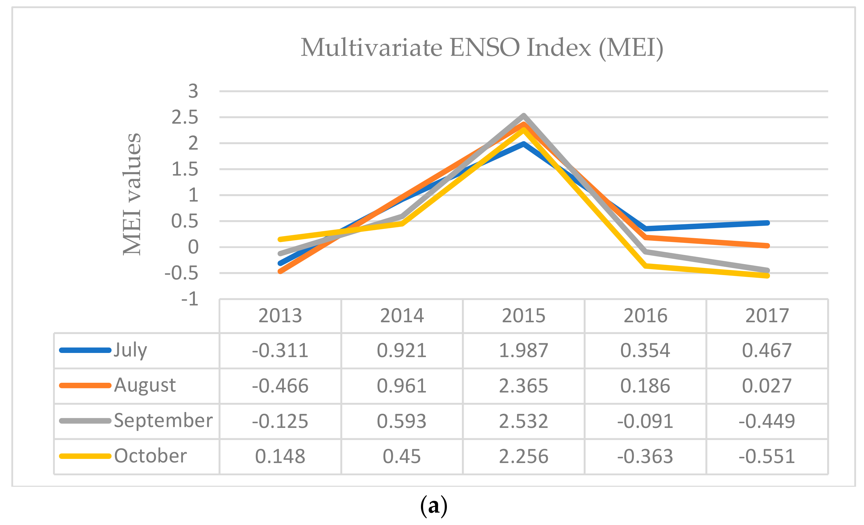
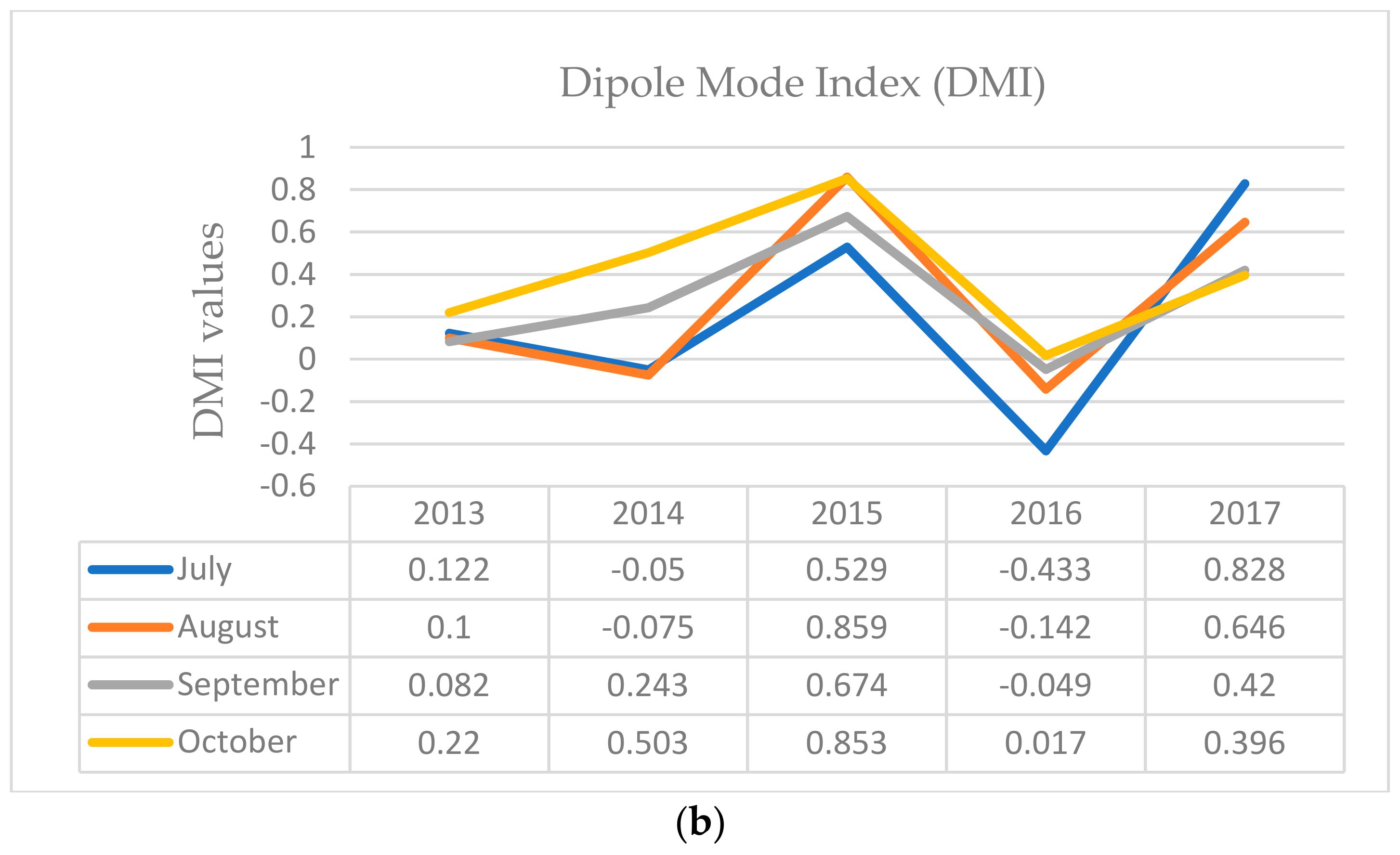
3.1. Concurrent ENSO and Positive IOD in 2015

Ocean-atmosphere interactions result ENSO in the Pacific Ocean and IOD in the Indian Ocean. Both phenomena can be generally identified by the surface air temperature anomaly and the impact can be seen on precipitation in the MC and around the world. The effects of single ENSO or IOD and their concurrent movement on an Indian summer monsoon have previously been identified [45]. Additionally, IOD influences the rainfall significantly and reduces the impact of ENSO while merging alongside. The BB episode of 2015 started in late July and lasted until late October. Therefore, MEI and DMI values are observed from July to October and 2013–2017 data are analyzed to understand how different 2015 was comparatively with the other years. Figure 2a,b illustrate that, in 2015, both MEI and DMI values were much higher comparatively with the other years and they coincided during the 2015 BB episode. It has been reported that El-Niño and positive IOD together caused a decrease in the rainfall and during the 2015 BB episode, the MC region saw below average precipitation [46]. By choosing the layer “Fires” from the NASA EOSDIS Worldview [34] and selecting dates during the 2015 BB episode, it can be seen how BB values intensified along with MEI and DMI. On the other hand, concurrence of La-Niña and negative IOD causes the opposite effect, which increases rainfall in the region.

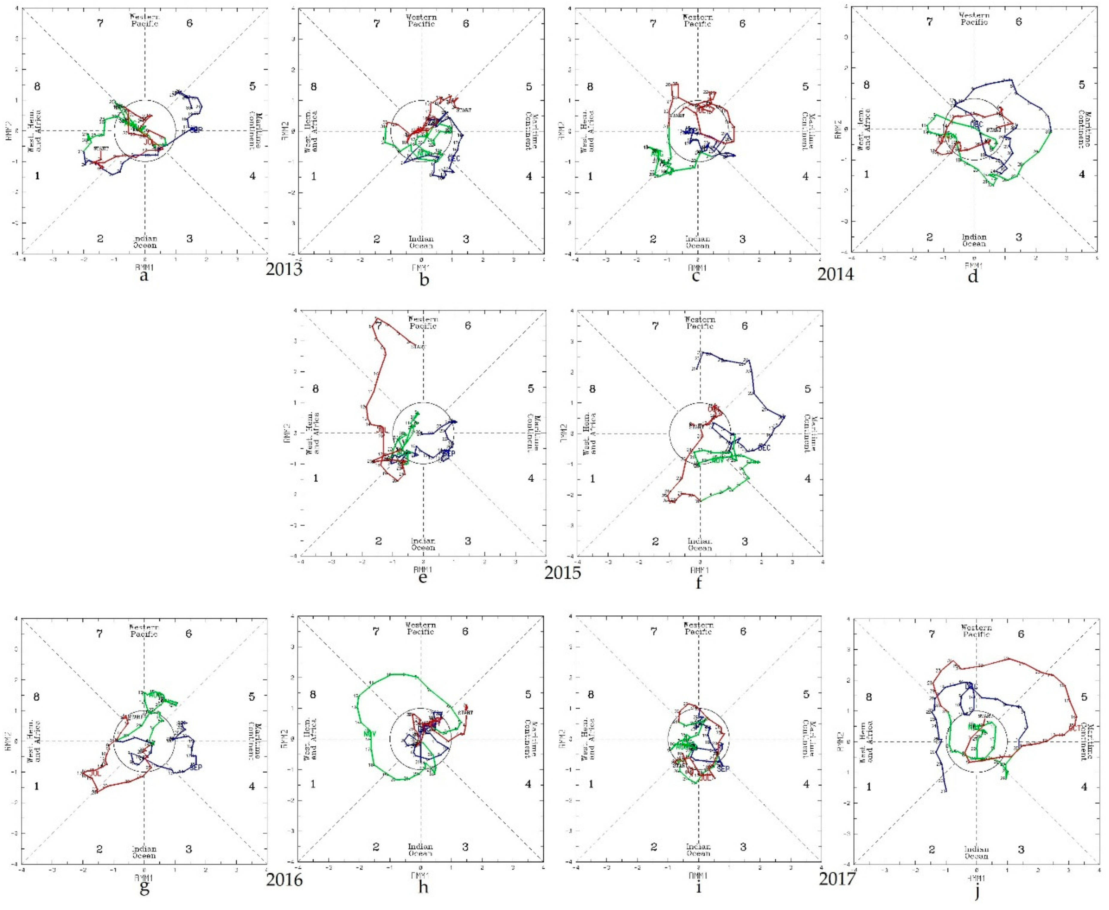
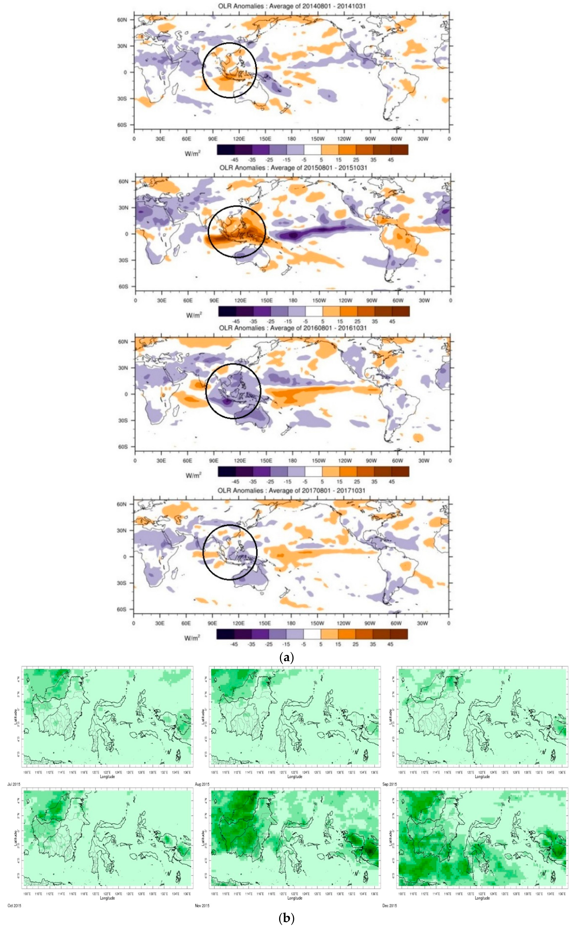
3.2. MJO, OLR, and Suppressed Rainfall during the 2015 BB Episode

MJO initially originates over the Indian Ocean and propagates eastward at a speed of 5 m s−1 through the tropical belt. It later passes through the MC region and finally decays over the date line in the Pacific Ocean [47]. Stronger and weaker MJO correspond to enhanced (convective) and suppressed rainfall respectively in the channel MJO passes through.
In Figure 3, MJO phases of 2013 to 2017 (July–December) are illustrated to compare 2015 MJO phases with the other years. The BB episode of 2015 in SEA started in late July and continued until mid-October [38]. Figure 3e shows the MJO phase during July–September and illustrates that the phase was strong at the beginning of July, but by the end of July the phase was located inside the circle, which clearly indicates that the MJO intensity became very weak (suppressed rainfall state). It continued until the end of September even though the MJO was passing through the MC only after mid-September. Figure 3f shows MJO phases during October–December where it is seen that, after mid-October, the MJO phases start getting stronger (enhanced rainfall state) while passing through the Indian Ocean and moving towards MC (easterly direction). Only in December 2015 the MJO phase passes through the MC with strong intensity and rainfall comes back to the MC. In addition, by the end of December 2015 the MJO phase ends up in the Western Pacific Ocean.
Figure 4a illustrates global outgoing longwave radiation (OLR) from August to October which highlights the regions experiencing cloudiness [33]. The circled mark in Figure 4a indicates our area of interest known as the MC. To study the 2015 BB episode, OLR data for other years (2014, 2016, and 2017) are compared with 2015 OLR datasets. Figure 4a clearly shows that the cloudiness during the BB period in 2015 is much lower when compared with other years. This connection of OLR with MJO of the same period (discussed above) indicate the drier season in MC.
Monthly rainfall analysis data (mm/month) of the MC [35] in Figure 4b is another connection of rainfall anomaly with MJO and OLR datasets from the 2015 BB episode. A rainfall anomaly from the July to December period is illustrated in Figure 4b where it is seen that rainfall over Sumatra and Kalimantan was far below average (350 to 600 mm/month) during the peak of the BB episode of 2015 (August–October) when the MJO intensity was very weak and OLR was very low. In November and December, the average precipitation rate came back to the MC when MJO intensity became stronger, which is illustrated in Figure 3f and OLR also became higher [31].

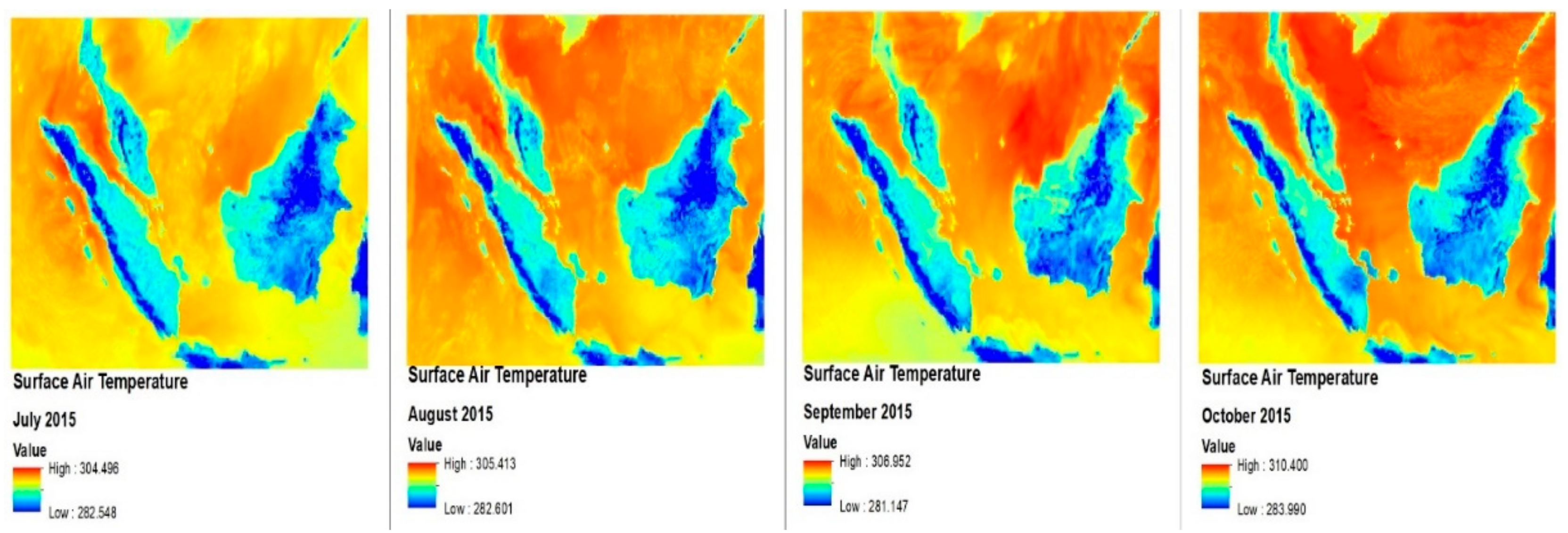
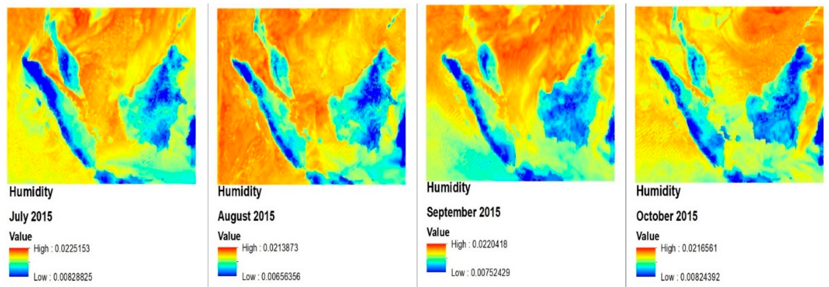
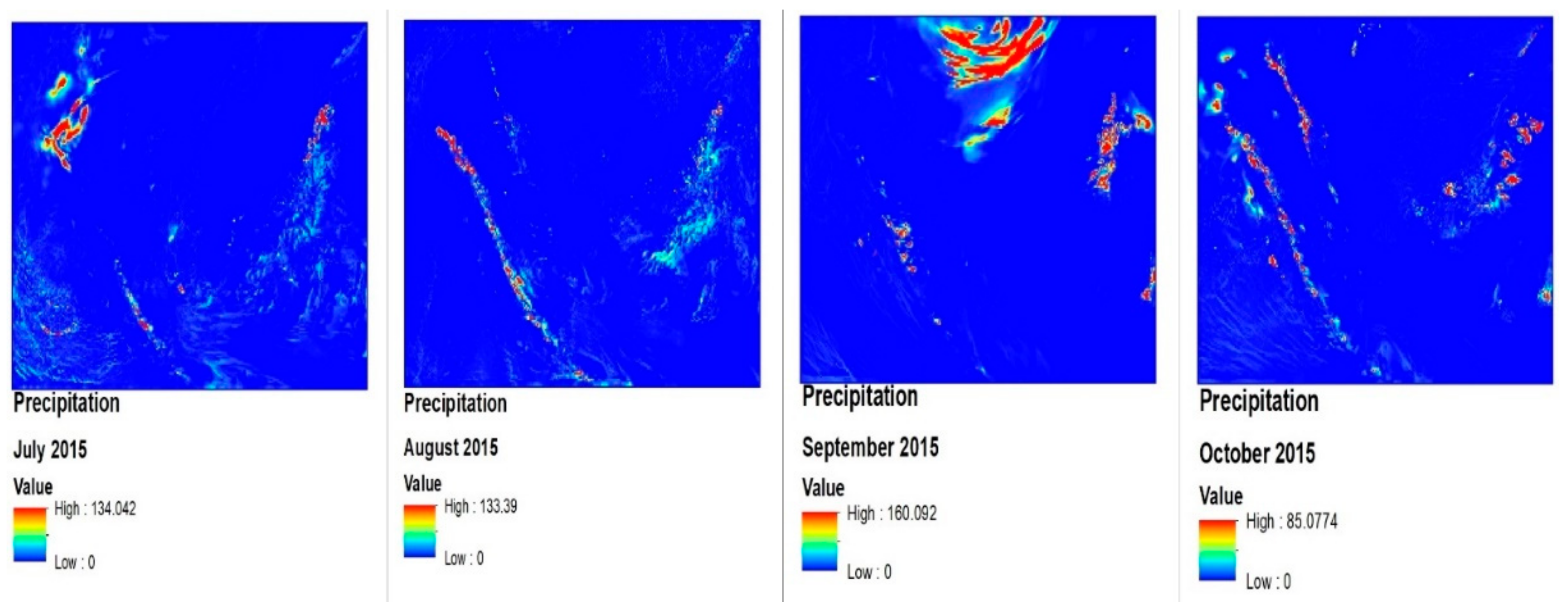
3.3. Model Data (Surface Air Temparature, Humidity, and Precipitation) Analysis from MEI, DMI, MJO, and OLR Viewpoints

WRF-ARW is run standalone for this study and no ocean model is coupled to it. Using the NWP model WRF-ARW, the following Figure 5 (for surface air temperature), Figure 6 (for humidity), and Figure 7 (for precipitation) are simulated.
Figure 5 shows that, throughout 2015 BB episode starting from July until October, the surface air temperature increased gradually from 304.496 K (31.346 °C (highest in July 2015) up to 310.4 K (37.25 °C (highest in October 2015) with RMSE ≈ 2.43. Higher surface air temperature makes the atmosphere less saturated and therefore, it reduces the humidity of the region. It causes a drier condition which exaggerates a suppressed conviction in the BB effected region. Figure 5 also shows a comparatively lower surface air temperature in the hilly areas in Malaysia, shoresides in western Sumatra, and densely covered forest areas in central Kalimantan, which are affected by the BB caused haze but remained unaffected from the actual forest burning of 2015.
Figure 6 is the NWP model simulated to investigate the humidity (water vapour pressure is considered, which is measured in millibars—mbar) of the BB affected area. The model simulation shows clearly how low the humidity is (<0.01 mb) in the affected area during the BB episode of 2015. The dark blue colour indicates where humidity is the least and it is the least during September–October of 2015 when BB is in peak.
Figure 7 illustrates the precipitation rate (rainfall) during the BB episode of 2015. The dark blue color represents very low precipitation. Table 2 shows (both observed and model values) that precipitation in the BB affected area is as low as <3 mm.
Figure 2a,b show that, in 2015, El-Niño and the positive phase of IOD merged concurrently. El-Niño kept intensifying from the beginning of the year with MEI value from July until September (1.987 < 2.365 < 2.532) and then slightly decreased later in October to 2.256. During the same time, the DMI value grew from 0.674 to 0.853. This analysis supports the statement that positive IOD reduces the impact of ENSO while merging concurrently [45].
Figure 3e shows, in the beginning of July 2015, how MJO starts moving from the Western Pacific region with a strong intensity. By the time it approaches the western hemisphere and Africa, the intensity starts becoming weaker and, by the end of July when it was approaching the Indian Ocean, it became very weak. This weak phase of MJO continues until the end of September and, by the end of September, the MJO was located at the centre of the circle, which means the MJO at that point in time is at its weakest possible state. This time, MJO passes across Indonesia through MC. This state of the MJO phase creates a much drier than average season in MC, which ends up with rainfall that is much lower than average (<3 mm). During this period, BB of 2015 was at its peak. This condition is also illustrated by the OLR diagram from Figure 4a of 2015 and by the rainfall data from July to September in Figure 4b. Figure 3f shows the MJO phase diagram of October to December 2015 where the MJO intensity keeps becoming stronger until mid-November. Later in November 2015, it becomes a little weaker and then keeps intensifying until the end of December through the MC. This resulted in an enhanced convection in MC and therefore, more rainfall occurred (Figure 4b, October–December), which mitigated the BB of the 2015 episode.

4. Conclusions

The study illustrates and emphasises that the BB episode of 2015 in Southeast Asia was strongly influenced by concurrence of ENSO and the positive IOD phenomenon, which increased the surface air temperature and made MC surroundings a hot bed for increased burning. The outgoing longwave radiation and MJO during the episode suppressed the convection and model data illustrating an extremely low precipitation rate during the BB episode. All these data conclude that the 2015 BB episode in MC was intensified by interconnected and interdependent climatic phenomena.
Several studies still need to be conducted to gain more detailed information. The mechanisms of El-Niño and positive IOD formation particularly for the 2015 episode still need to be studied. We need better understanding regarding the non-uniform rainfall response during El-Niño in the boreal winter and the boreal summer. Whether direct linear or non-linear links exist among ENSO, IOD, and MJO or not is also a big question. How the vast haze formed due to the BB in 2015, propagated through the MC, and how it impacted the regional climate also need to be investigated.

Author Contributions

M.A.I. designed and performed the simulation and wrote the paper. C.G.O. co-designed and provided a critical revision. M.A. contributed to the ground observation data collection and analysing the data. M.J.A. contributed to the conception, design of the study, and provided critical revision. A.C. designed the project, ensured the accuracy of the article, and provided final approval of the version to be submitted for publication.

Funding

The study is supported by the Malaysian Ministry of Science, Technology and Innovation (MOSTI) under project: “Biomass burning haze (BBH) in Southeast Asia (SEA): Development of a computational tool to predict its transport and impacts on climate change in Malaysia”, contract number 06-02-12-SF0346.

Acknowledgments

The model computations were run on the cluster supported by the High-Performance Computing (HPC) facility of the University of Nottingham, UK campus.

Conflicts of Interest

The authors declare no conflicts of interest.

References

  1. Ramage, C.S. Role of a tropical maritime continent in the atmospheric circulation 1. Mon. Weather Rev. 1968, 96, 365–370. [Google Scholar] [CrossRef]
  2. Richard, N.; Jilia, S. The Maritime Continent and Its Role in the Global Climate: A GCM Study. J. Clim. 2003, 16, 834–848. [Google Scholar] [CrossRef]
  3. Chang, C.-P.; Zhuo, W. Annual Cycle of Southeast Asia—Maritime Continent Rainfall and the Asymmetric Monsoon Transition. J. Clim. 2005, 18, 287–301. [Google Scholar] [CrossRef] [Green Version]
  4. Qian, J.-H. Why Precipitation Is Mostly Concentrated over Islands in the Maritime Continent. J. Atmosp. Sci. 2008, 67, 3509–3524. [Google Scholar] [CrossRef]
  5. Pike, A.C. Intertropical convergence zone studied with an interacting atmosphere and ocean model. Mon. Weather Rev. 1971, 99, 469–477. [Google Scholar] [CrossRef]
  6. Gianotti, R.L. Assessment of the Regional Climate Model Version 3 over the Maritime Continent Using Different Cumulus Parameterization and Land Surface Schemes. J. Clim. 2012, 25, 638–656. [Google Scholar] [CrossRef]
  7. Aldrian, E.; Susanto, R.D. Identification of three dominant rainfall regions within Indonesia and their relationship to sea surface temperature. Int. J. Climatol. 2003, 23, 1435–1452. [Google Scholar] [CrossRef] [Green Version]
  8. Rakhmat, P.; As-Syakur, R.A.; Takahiro, O. Validation of TRMM Precipitation Radar satellite data over Indonesian region. Theor. Appl. Climatol. 2013, 12, 575–587. [Google Scholar]
  9. Zhong, L. Tropical Rainfall Measuring Mission (TRMM) Precipitation Data and Services for Research and Applications. Bull. Am. Meteorol. Soc. 2012, 92, 1317–1325. [Google Scholar] [CrossRef]
  10. Giannini, A.; Robertson, A.W.; Qian, J.H. A role for tropical tropospheric temperature adjustment to El-Niño Southern Oscillation in the seasonality of monsoonal Indonesia precipitation predictability. J. Geophys. Res.: Atmosp. 2007, 112, 1–14. [Google Scholar] [CrossRef]
  11. Andreae, P.J.; Crutzen, M.O. Biomass burning in the tropics: Impact on atmospheric chemistry and biogeochemical cycles. Science 1990, 250, 1669–1678. [Google Scholar] [CrossRef]
  12. Van der Werf, G.R.; Randerson, J.T.; Giglio, L.; Collatz, G.J.; Mu, M.; Kasibhatla, P.S.; Morton, D.C.; DeFries, R.S.; Jin, Y.; van Leeuwen, T.T. Global fire emissions and the contribution of deforestation, savanna, forest, agricultural, and peat fires (1997–2009). Atmos. Chem. Phys. 2010, 10, 11707–11735. [Google Scholar] [CrossRef] [Green Version]
  13. Field, R.D.; der werf, G.R.V.; Fanin, T.; Fetzer, E.J.; Fuller, R.; Jethva, H.; Levy, R.; Livesey, N.J.; Luo, M.; Torres, O.; et al. Indonesian fire activity and smoke pollution in 2015 show persistent nonlinear sensitivity to El-Niño induced drought. Proc. Natl. Acad. Sci. USA 2016, 113, 9204–9209. [Google Scholar] [CrossRef] [PubMed]
  14. Islam, M.S.; Pei, Y.H.; Mangharam, S. Trans-Boundary Haze Pollution in Southeast Asia: Sustainability through Plural Environmental Governance. Sustainability 2016, 8, 499. [Google Scholar] [CrossRef]
  15. Okimori, Y.; Ogawa, M.; Takahashi, F. Potential of Co2 emission reductions by carbonizing biomass waste from industrial tree plantation in South Sumatra, Indonesia. Mitig. Adapt. Strateg. Glob. Chang. 2003, 8, 261–280. [Google Scholar] [CrossRef]
  16. Janssens-Maenhout, G.; Crippa, M.; Guizzardi, D.; Muntean, M.; Schaaf, E.; Olivier, J.; Peters, J.; Schure, K. Fossil CO2 & GHG Emissions of All World Countries; JRC (Joint Research Centre) Science for Policy Report; JRC (Joint Research Centre): Ispra, Italy, 2018; ISBN 978-92-79-73207-2. [Google Scholar]
  17. Chen, J.; Li, C.; Ristovski, Z.; Milic, A.; Gu, Y.; Islam, M.S.; Wang, S.; Hao, J.; Zhang, H.; He, C.; et al. A review of biomass burning: Emissions and impacts on air quality, health and climate in China. Sci. Total Environ. 2017, 579, 1000–1034. [Google Scholar] [CrossRef] [PubMed]
  18. Zhu, Z. Breakdown of the relationship between Australian summer rainfall and ENSO caused by tropical Indian Ocean SST warming. J. Clim. 2018, 31, 2321–2336. [Google Scholar] [CrossRef]
  19. Zhu, Z.; Li, T.; He, J. Out-of-Phase Relationship between Boreal Spring and Summer Decadal Rainfall Changes in Southern China. J. Clim. 2013, 27, 1083–1099. [Google Scholar] [CrossRef]
  20. Saha, K. Tropical Circulation Systems and Monsoons; Springer: Berlin, Germany, 2010. [Google Scholar]
  21. Jiang, L.; Li, T. Why rainfall response to El Niño over Maritime Continent is weaker and non-uniform in boreal winter than in boreal summer. Clim. Dyn. 2018, 51, 1465–1483. [Google Scholar] [CrossRef]
  22. McBride, J.L.; Haylock, M.R.; Nicholls, N. Relationships between the Maritime Continent Heat Source and the El Niño–Southern Oscillation Phenomenon. J. Clim. 2003, 16, 2905–2914. [Google Scholar] [CrossRef] [Green Version]
  23. Haylock, M.; McBride, J. Spatial Coherence and Predictability of Indonesian Wet Season Rainfall. J. Clim. 2001, 14, 3882–3887. [Google Scholar] [CrossRef]
  24. Zhang, C. Madden–Julian Oscillation: Bridging Weather and Climate. Bull. Am. Meteorol. Soc. 2013, 94, 1849–1870. [Google Scholar] [CrossRef]
  25. Oh, J.H.; Kim, B.M.; Kim, K.Y.; Song, H.J.; Lim, G.H. The impact of the diurnal cycle on the MJO over the Maritime Continent: A modeling study assimilating TRMM rain rate into global analysis. Clim. Dyn. 2012, 40, 893–911. [Google Scholar] [CrossRef]
  26. Mazzarella, A.; Giuliacci, A.; Scafetta, N. Quantifying the Multivariate ENSO Index (MEI) coupling to CO2 concentration and to the length of day variations. Theor. Appl. Climatol. 2012, 111, 601–607. [Google Scholar] [CrossRef]
  27. Wolter, K.; Timlin, M.S. Monitoring ENSO in COADS with a Seasonally Adjusted Principal Component Index. University of Oklahoma, School of Meteorology. Norman: Oklahoma Climate Survey. Available online: https://www.esrl.noaa.gov/psd/enso/mei/WT1.pdf (accessed on 15 June 2018).
  28. Saji, N.H.; Yamagata, T. Possible impacts of Indian Ocean Dipole mode events on global climate. Clim. Res. 2003, 25, 151–169. [Google Scholar] [CrossRef] [Green Version]
  29. ESRL/NOAA. (12 September 2017). Dipole Mode Index (DMI). Retrieved from Global Climate Observing System (GCOS). Available online: https://www.esrl.noaa.gov/psd/gcos_wgsp/Timeseries/Data/dmi.long.data (accessed on 17 May 2018).
  30. Wheeler, M.C.; Harry, H.H. An All-Season Real-Time Multivariate MJO Index: Development of an Index for Monitoring and Prediction. Mon. Weather Rev. 2004, 132, 1917–1932. [Google Scholar] [CrossRef] [Green Version]
  31. Bureau of Meteorology, Australia. Madden-Julian Oscillation (MJO). Retrieved from Bureau of Meteorology, Australia. Available online: http://www.bom.gov.au/climate/mjo/#tabs=MJO-phase (accessed on 17 May 2018).
  32. Petty, G.W. A First Course in Atmospheric Radiation, 2nd ed.; Sundog Publishing: Madison, WI, USA, 2006. [Google Scholar]
  33. Bureau of Meteorology, Australia. Global Maps of Outgoing Longwave Radiation (OLR). Melbourne, Victoria, Australia. Available online: http://www.bom.gov.au/climate/mjo/#tabs=Cloudiness (accessed on 1 May 2018).
  34. NASA Earthdata-EOSDIS. Global Fire Maps. Retrieved from NASA Worldview. Available online: https://worldview.earthdata.nasa.gov/?p=geographic&l=MODIS_Aqua_SurfaceReflectance_Bands143,MODIS_Aqua_SurfaceReflectance_Bands721,MODIS_Terra_SurfaceReflectance_Bands143,MODIS_Terra_SurfaceReflectance_Bands721,VIIRS_SNPP_CorrectedReflectance_TrueColor(hi (accessed on 15 May 2018).
  35. Joyce, R.J.; Janowiak, J.E.; Arkin, P.A.; Xie, P. CMORPH: A Method that Produces Global Precipitation Estimates from Passive Microwave and Infrared Data at High Spatial and Temporal Resolution. J. Hydrometeorol. 2004, 5, 487–503. [Google Scholar] [CrossRef]
  36. National Centers for Environmental Prediction/National Weather Service/NOAA/U.S. Department of Commerce (2015): NCEP GDAS/FNL 0.25 Degree Global Tropospheric Analyses and Forecast Grids. Research Data Archive at the National Center for Atmospheric Research, Computational and Information Systems Laboratory. Dataset. Available online: https://doi.org/10.5065/D65Q4T4Z (accessed on 10 May 2018).
  37. NOAA. Bimonthly MEI Values. Retrieved from Multivariate ENSO Index (MEI). Available online: https://www.esrl.noaa.gov/psd/enso/mei/table.html (accessed on 17 May 2018).
  38. Hong, S.-Y.; Dudhia, J.; Chen, S.-H. A Revised Approach to Ice Microphysical Processes for the Bulk Parameterization of Clouds and Precipitation. Mon. Weather Rev. 2004, 132, 103–120. [Google Scholar] [CrossRef] [Green Version]
  39. Mlawer, E.J.; Taubman, S.J.; Brown, P.D.; Iacono, M.J.; Clough, S.A. Radiative transfer for inhomogeneous atmospheres: RRTM, a validated correlated-k model for the longwave. J. Geophys. Res. 1997, 102, 16663–16682. [Google Scholar] [CrossRef] [Green Version]
  40. Dudhia, J. Numerical Study of Convection Observed during the Winter Monsoon Experiment Using a Mesoscale Two-Dimensional Model. J. Atmos. Sci. 1989, 46, 3077–3107. [Google Scholar] [CrossRef] [Green Version]
  41. Monin, A.S.; Obukhov, A.F.M. Basic laws of turbulent mixing in the surface layer of the atmosphere. Contrib. Geophys. Inst. Acad. Sci. 1954, 24, 163–187. [Google Scholar]
  42. Niu, G.-Y.; Yang, Z.-L.; Mitchell, K.E.; Chen, F.; Ek, M.B.; Barlage, M.; Kumar, A.; Manning, K.; Niyogi, D.; Rosero, E.; et al. The community Noah land surface model with multiparameterization options (Noah-MP): 1. Model description and evaluation with local-scale measurements. J. Geophys. Res. 2011, 116, 1–19. [Google Scholar] [CrossRef]
  43. Hong, S.-Y.; Noh, Y.; Dudhia, J. A new vertical diffusion package with an explicit treatment of entrainment processes. Mon. Weather Rev. 2006, 134, 2318–2341. [Google Scholar] [CrossRef]
  44. Kain, J.S. The Kain–Fritsch Convective Parameterization: An Update. J. Appl. Meteorol. 2004, 43, 170–181. [Google Scholar] [CrossRef]
  45. Ashok, K.; Guan, Z. Individual and Combined Influences of ENSO and the Indian Ocean Dipole on the Indian Summer Monsoon. J. Clim. 2004, 17, 3141–3155. [Google Scholar] [CrossRef]
  46. Meyers, G.; McIntosh, P.; Pigot, L.; Pook, M. The Years of El Niño, La Niña, and interactions with the tropical Indian Ocean. J. Clim. 2007, 20, 2872–2880. [Google Scholar] [CrossRef]
  47. Zhang, C. Madden-julian oscillation. Rev. Geophys. 2005, 43, 1–36. [Google Scholar] [CrossRef]
Figure 1. Selected zone of our study for running the NWP model with WRF-ARW. Figure shows the land (red) and water body (blue) of Malaysia and part of Indonesia (Sumatra and Kalimantan), which is the main region where the BB episode occurred in 2015. The computer model is run also in this selected zone.
Atmosphere 09 00352 g001
Figure 2. (a) Multivariate ENSO Index (MEI) data [37] show the values during July–October (2013–2017). The graph shows that the highest MEI values were in 2015. In September 2015, the MEI value was highest when the BB of 2015 episode was also in its peak. (b) Dipole Mode Index (DMI) [29] values are shown in the graphs for 2013–2017. Positive IOD with higher DMI values in 2015 are concurrent with a higher MEI during the same period, which intensified the BB episode.
Atmosphere 09 00352 g002aAtmosphere 09 00352 g002b
Figure 3. MJO phases (2013–2017) of six months (July–December) in two stages (July–September) in (a), (c), (e), (g), (i), and (October–December) in (b), (d), (f), (h), (j) shown using the RMM1 and RMM2 (Real-time Multivariate MJO) method [30] from 2013 to 2017 [31]. Each month in the phase diagram starts with red, continues the next month with green, and ends with a blue line. The inner circle in each phase diagram represents area where MJO intensity is weakest. As the MJO phase line goes far from the inner circle, the intensity increases.
Atmosphere 09 00352 g003
Figure 4. (a) Outgoing longwave radiation (OLR), W m−2 anomalies from 2014 until 2017 (August–October) [33]. Blue shading indicates cloudiness above normal and brown shading indicates cloudiness below normal. The circled part is the area of the study that shows that August to October of 2015 was the driest period, which accordingly, was also the peak of BB of that year. (b) Monthly rainfall analysis data (mm/month) in MC [33]. Figure shows rainfall data from July to December 2015 in the Indonesia region. The light green color shows below normal data and the dark green color shows the above normal data respectively. It is seen that, during the BB period (August–October) in the affected area (Malaysia, Sumatra, and Kalimantan), precipitation was extremely low, which provoked the intensification of BB. In November and December the precipitation came back to the region which mitigated the BB.
Atmosphere 09 00352 g004
Figure 5. Mean surface air temperature during July–October 2015. Figure shows Malaysia, Sumatra, and the Kalimantan region simulated and the temperature of their surrounding surface area during BB of 2015. The temperature went up as high as 310.4 K (37.25 °C), which is covered by a dark orange shade, and as low as 303.48 K (30.33 °C), which is covered by a yellow shade. The temperature range was above normal during the BB episode.
Atmosphere 09 00352 g005
Figure 6. The simulated model shows humidity of the BB affected area of MC in 2015 during July–October. Dark orange and dark blue colors indicate the highest and lowest values, respectively. Figures illustrate the main BB affected area (Central Sumatra and Southern Kalimantan) had very low humidity when BB was in peak (September–October 2015).
Atmosphere 09 00352 g006
Figure 7. The Simulated precipitation rate (rainfall) in Sumatra, Kalimantan, and the Malaysia region. It shows rainfall data from July to October 2015. Dark blue indicates extremely low rainfall, which was less than 3 mm (see Table 2) during the 2015 BB episode. Therefore, the whole child domain (selected MC region of our study) is covered with a dark blue color in the model. Some areas show higher precipitation (dark orange color), which were not affected by BB in 2015.
Atmosphere 09 00352 g007
Table 1. Settings and configurations used for the WRF-ARW model.
Physics (Processes)Schemes Description
Microphysics schemeWRF single-Moment (WSM) 3-class [38]
Long-wave radiation schemeRRTM (Rapid Radiative Transfer Model) scheme [39]
Short-wave radiation schemeDudhia scheme [40]
Surface layer schemeMonin-Obukhov similarity scheme [41]
Land surface modelNoah-MP Land Surface model [42]
Planetary boundary layer (PBL) schemeYonsei University scheme (YSU) [43]
Cumulus parameterization schemeKain-Fritsch (new Eta) scheme [44]
Table 2. RMSE calculation for surface air temperature (K), and precipitation (mm). The table describes the MSE and RMSE calculation process. The calculated values of RMSE for surface air temperature and precipitation are 2.43 and 0.49, respectively.
2015
(SST)
K
Observed Value (Mean)
Oi
Model Value (Mean)
Mi
Absolute Error
|(Oi−Mi)|
Square of the Absolute Error
|(Oi−Mi)|2
MSERMSE
Months5.9≈2.43
JUL303.48300.92.56.25
AUG303.65301.22.56.07
SEP303.38300.92.56.18
OCT303.85301.62.35.19
2015
(Precipitation) mm
Observed Value (Mean)
Oi
Model Value (Mean)
Mi
Absolute Error
|(Oi−Mi)|
Square of the Absolute Error
|(Oi−Mi)|2
MSERMSE
Months0.24≈0.49
JUL1.741.150.590.35
AUG1.381.170.210.04
SEP1.901.300.630.40
OCT2.632.250.380.15

