Article

Using a Backpropagation Artificial Neural Network to Predict Nutrient Removal in Tidal Flow Constructed Wetlands

1
Institute of Wetland Research, Chinese Academy of Forestry, Beijing 100091, China
2
The Beijing Key Laboratory of Wetland Ecological Function and Restoration, Beijing 100091, China
3
Beijing Hanshiqiao National Wetland Ecosystem Research Station, Beijing 101399, China
*
Author to whom correspondence should be addressed.
Water 2018, 10(1), 83; https://doi.org/10.3390/w10010083
Submission received: 3 November 2017 / Revised: 2 January 2018 / Accepted: 14 January 2018 / Published: 18 January 2018

Abstract

:
Nutrient removal in tidal flow constructed wetlands (TF-CW) is a complex series of nonlinear multi-parameter interactions. We simulated three tidal flow systems and a continuous vertical flow system filled with synthetic wastewater and compared the influent and effluent concentrations to examine (1) nutrient removal in artificial TF-CWs, and (2) the ability of a backpropagation (BP) artificial neural network to predict nutrient removal. The nutrient removal rates were higher under tidal flow when the idle/reaction time was two, and reached 90 ± 3%, 99 ± 1%, and 58 ± 13% for total nitrogen (TN), ammonium nitrogen (NH4+-N), and total phosphorus (TP), respectively. The main influences on nutrient removal for each scenario were identified by redundancy analysis and were input into the model to train and verify the pollutant effluent concentrations. Comparison of the actual and model-predicted effluent concentrations showed that the model predictions were good. The predicted and actual values were correlated and the margin of error was small. The BP neural network fitted best to TP, with an R2 of 0.90. The R2 values of TN, NH4+-N, and nitrate nitrogen (NO3-N) were 0.67, 0.73, and 0.69, respectively.

1. Introduction

In recent decades, constructed wetlands have been widely used to treat industrial and agricultural wastewater because of their ability to remove nutrients, organic matter, heavy metals, and pathogens from wastewater [1,2,3]. In addition to their wastewater purification ability, constructed wetlands have low running costs, low energy consumption, and are simple to manage and maintain [4,5,6]. However, constructed wetlands are also criticized for their low re-oxygenation ability and their vulnerability to low temperatures, so it is therefore necessary to find methods and technologies for improving existing constructed wetlands.
A new type of constructed wetland system, a tidal flow constructed wetland (TF-CW), has significantly higher dissolved oxygen (DO) levels than conventional constructed wetlands [7]. The TF-CW uses the interstitial suction created by a change in the bed infiltration surface during tidal operations to suck atmospheric oxygen into the wetland matrix or soil voids [8,9]. Through this mechanism, the oxygen environment in the bed of the artificial wetland can be improved considerably, such that the plant roots have sufficient oxygen. The TF-CW also provides more efficient removal of ammonium nitrogen (NH4+-N) and organic matter than traditional constructed wetlands. Nutrient removal in constructed wetlands is linked to many factors. For example, NH4+-N removal is influenced by, among other factors, the influent concentration, temperature, pH, and DO. The removal of nitrate nitrogen (NO3-N) is influenced by total organic carbon (TOC), the influent method, and time [10,11]. The removals of NH4+-N and NO3-N are linked, and are influenced, promoted, or restricted by these factors, resulting in a complex artificial wetland ecosystem. Pollutant removal in TF-CWs is therefore a complex process involving nonlinear multi-parameter interactions [12].
Rumelhart and McCelland established a multi-layer feed-forward neural network trained by an error backpropagation algorithm in 1986, known as the backpropagation (BP) network, which later become one of the most widely used neural network models. These BP networks can learn and store many input–output pattern mappings and can predict the complex dynamic systems of nonlinear models [13]. The applications of BP neural networks infiltrate into various disciplines; for example, they can be used to predict disasters such as typhoon pathways [14] and earthquakes [15], to classify remote sensing images [16], identify wireless channels [17], predict the stock market [18], and to predict groundwater quality [19]. In ecology, BP neural networks are widely used, for example, to support ecological and environmental health assessments [20,21], ecological planning, ecological security assessment, eco-environmental quality assessment, ecological restoration, and pest prediction [22,23,24]. However, they have rarely been applied to predict the performance of TF-CWs. In this study, we set up a BP network model to predict the removal of pollutants from TF-CWs with four different influent modes. We used this model to construct the artificial neural network topological structure of constructed wetlands, to further simulate the process of TF-CWs, and to validate the concentrations of nitrogen and phosphorus in effluents. The aim of this study was to predict the quality of the effluent discharged from TF-CWs and to optimize the nitrogen and phosphorus removal efficiencies.

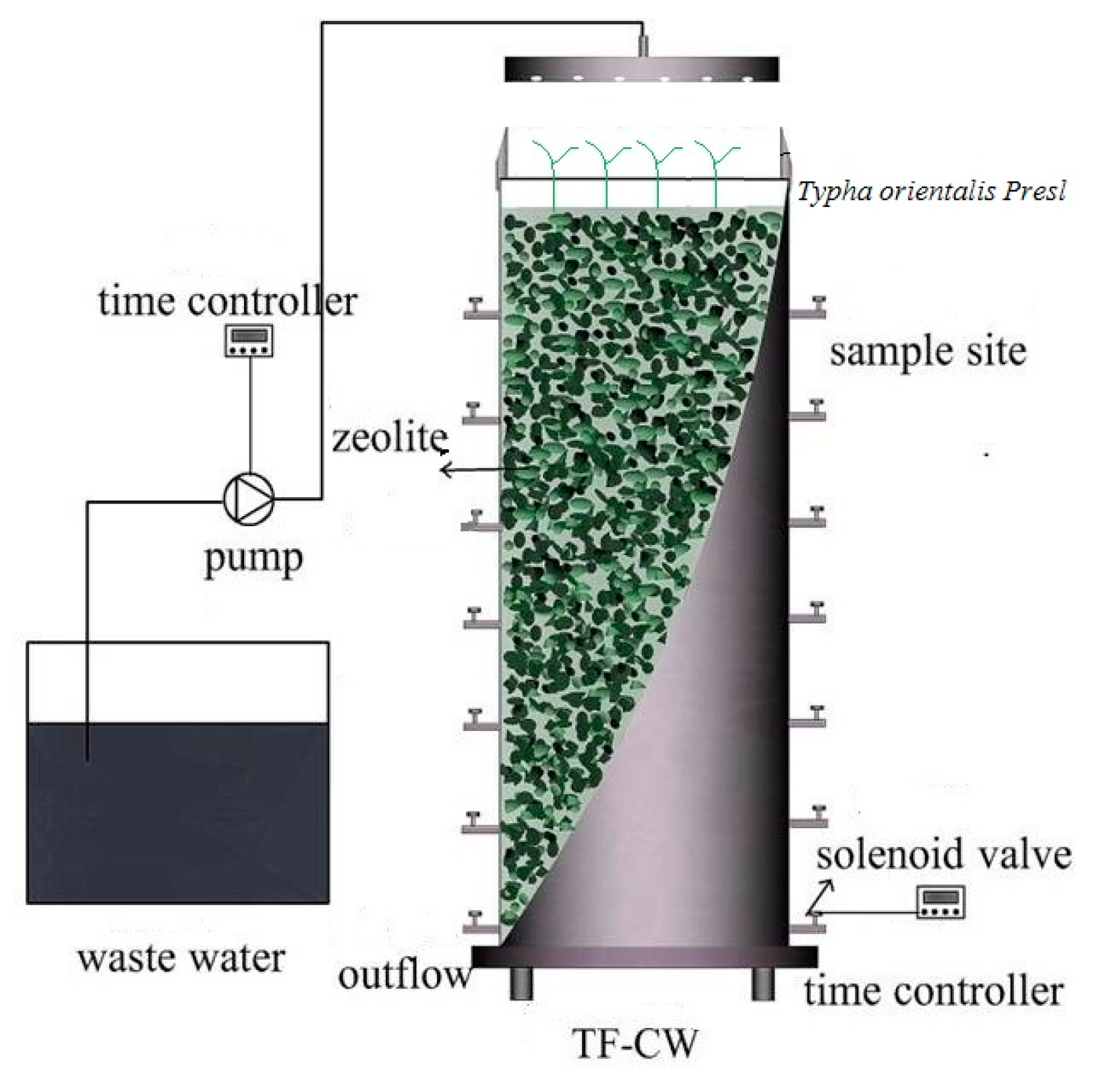
2. Materials and Methods

The TF-CW simulator (Beijing, China) used in this study was a cylindrical steel drum, 110 cm high, with a diameter and volume of 40 cm and 138 L, respectively (Figure 1). The device had 21 sampling ports, each with a diameter of 1 cm. These ports were equally spaced around the device in seven rows that were arranged at 15-cm intervals from the top to the bottom. The inflow water was controlled by a water pump that was monitored by a time controller (TB-125, LUEABB, Wenzhou, China). The device was covered with a sprinkler cover that had small holes on its bottom to ensure uniform water flow. The effluent water was controlled by electromagnetic valve (2 W normally closed 220 V, LUEABB, Wenzhou, China) and was monitored by a time controller. Zeolite, with a particle size of between 4 and 8 mm and a porosity of 42%, was filled into the device to a height of 105 cm. The zeolite was planted with Typha orientalis.
We simulated the sewage of Beijing using ammonium chloride, glucose, and monopotassium phosphate to represent total nitrogen (TN), TOC, and total phosphorus (TP), respectively. The volume of artificial sewage stored was 4 m3. The concentrations of the main water quality indicators in the simulated sewage are shown in Table 1.
In this experiment, we studied the effects of nutrient removal and the factors that influenced nutrient removal under different influent modes in four test devices (A–D). We set up three different tidal water inflow models (B, C, and D), and a continuous influent mode as a control (A). The input cycle of the four modes was 24 h. Each of the four installations received the same amount of flow (0.138 m3/day). Details of the hours of operation are presented in Table 2. We conducted a preliminary experiment from January to March 2014. We then attached the membrane to the substrate and commenced the experiment formally in April 2014.
Water samples from the sampling ports at seven treatment depths (15, 30, 45, 60, 75, 90, and 105 cm) in Devices A, B, C, and D and the sewage pool were collected weekly from April 2014 to November 2014 and sent to the laboratory for analysis. Temperature, DO, oxidation reduction potential (ORP), pH, and conductivity (Cond) were measured by a portable multi-parameter water quality analyzer (YSI-EXO, YSI, Yellow Springs, OH, USA). The concentrations of TN, NH4+-N, nitrite nitrogen (NO2-N), NO3-N, and TP were determined by an automatic discrete analyzer (SMARTCHEM200, WestCo, Frepillon, France).
We used Origin 8.5 (OriginLab, Northampton, MA, USA) for data fitting and SPSS version 19.0 (SPSS, Chicago, IL USA) for statistical analysis. Statistically significant differences were determined at the α = 0.05 significance level. RDA analyses were carried out within Canoco4.5 (Microcomputer Power, Ithaca, NY, USA) and we constructed the plot in CanoDraw4.5 (Microcomputer Power, Ithaca, NY, USA). The BP neural network was simulated in Matlab R2011b (MathWorks, Natick, MA, USA).

3. Results and Discussion

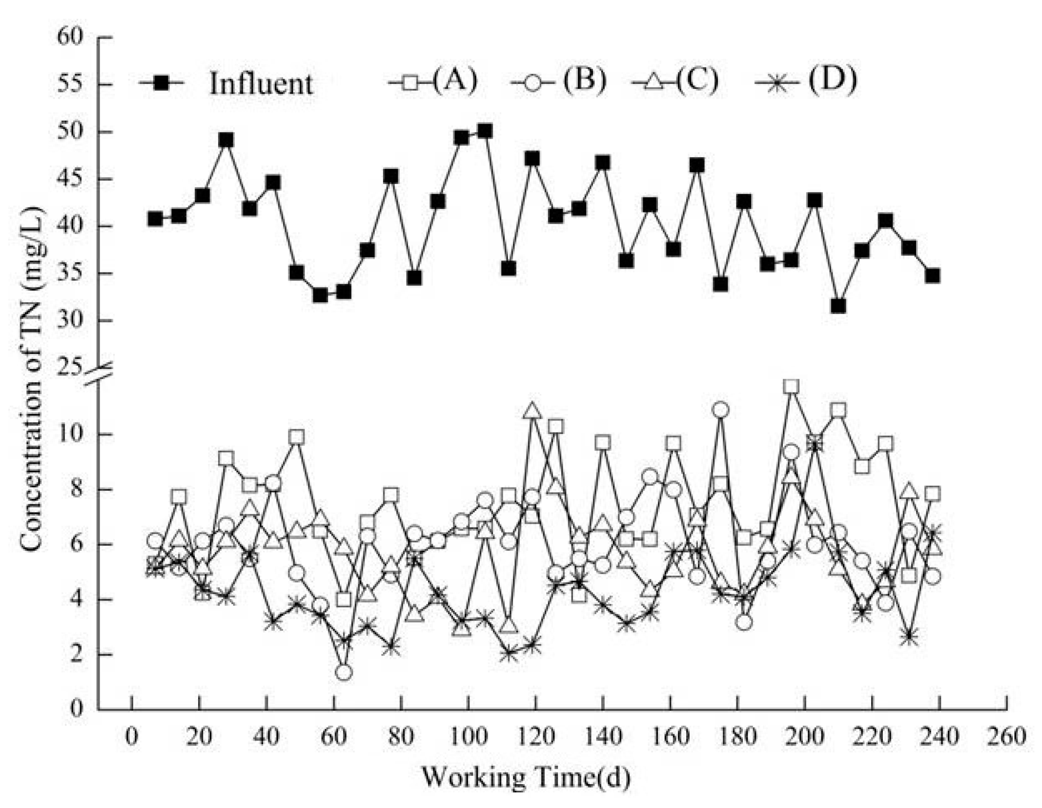
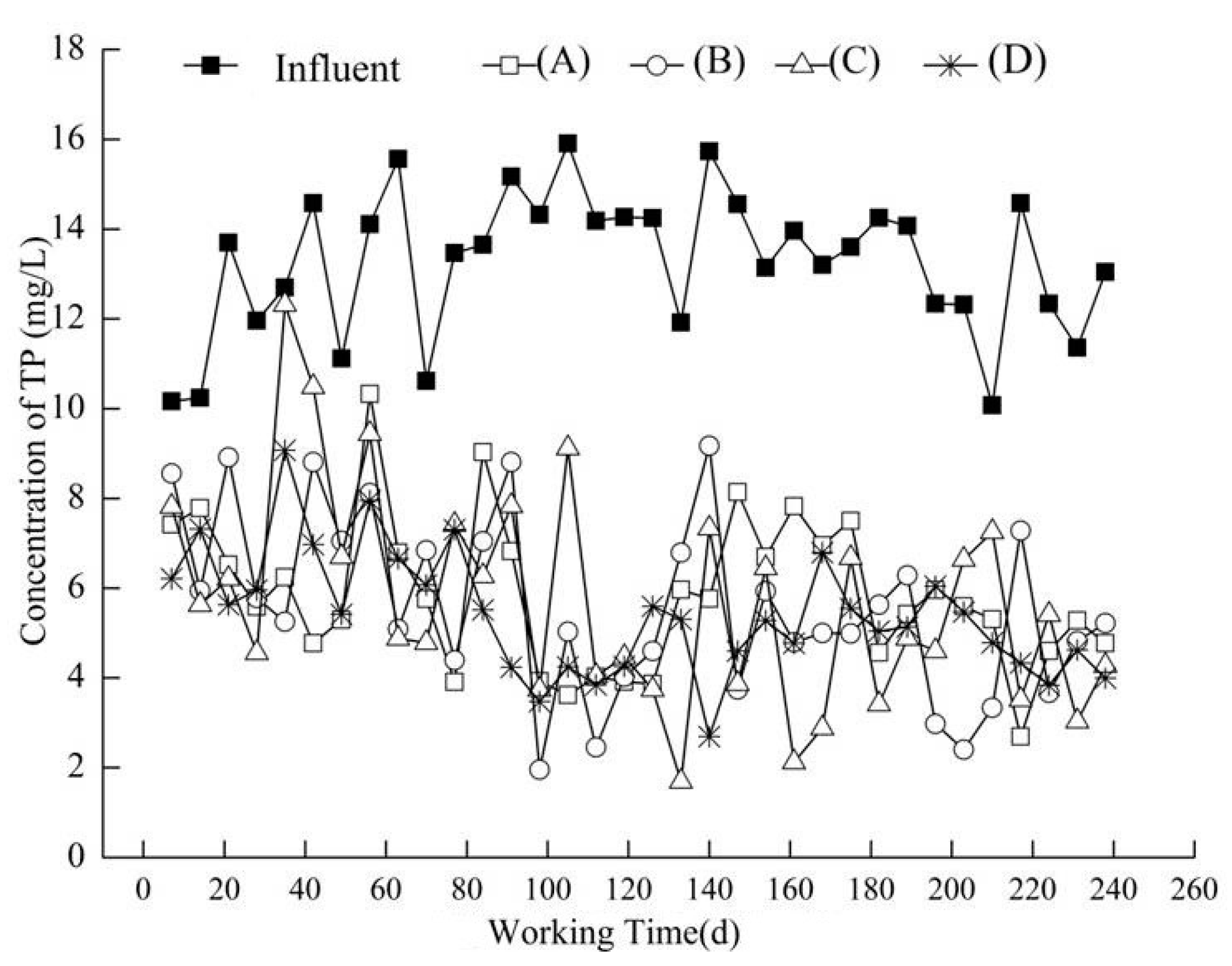
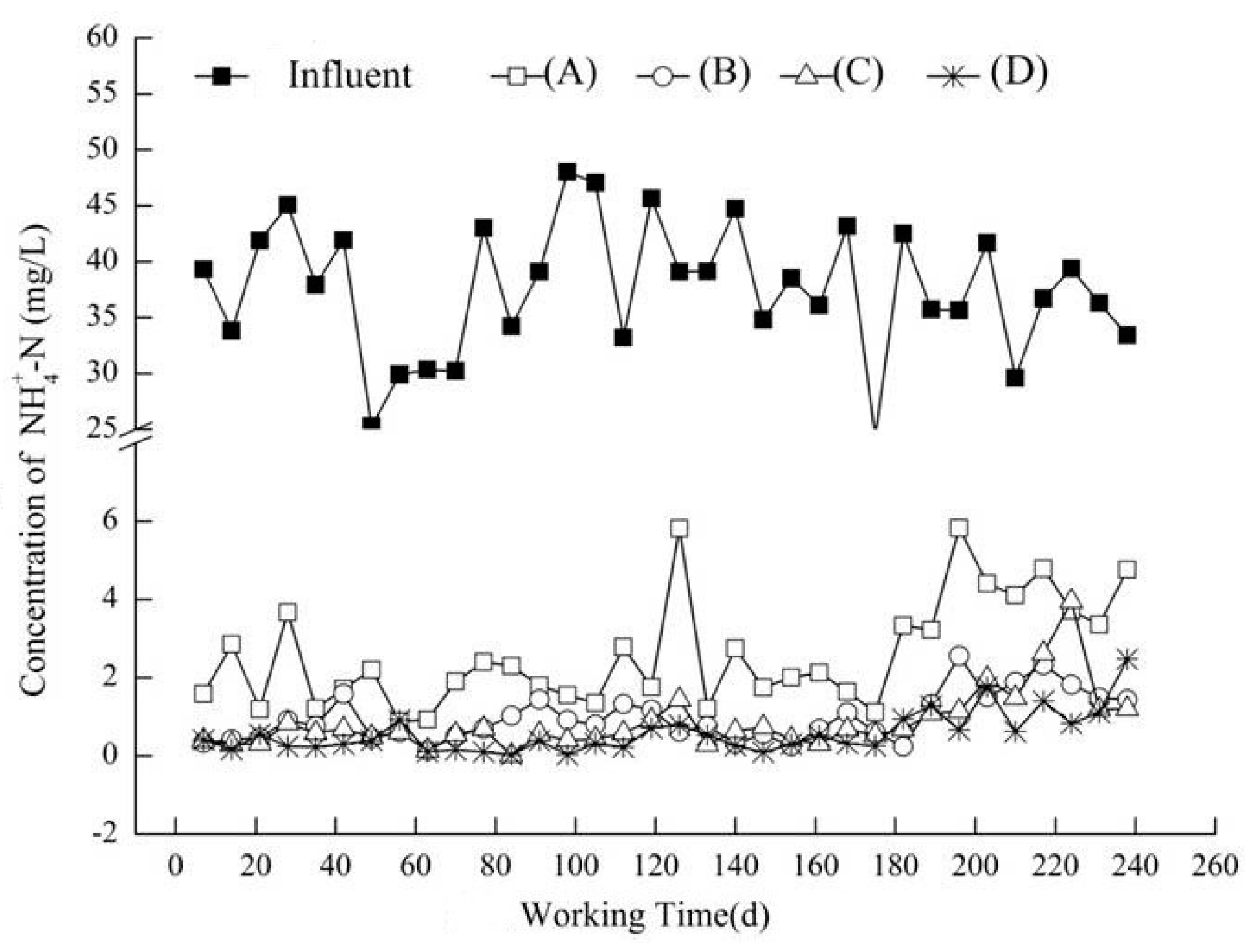
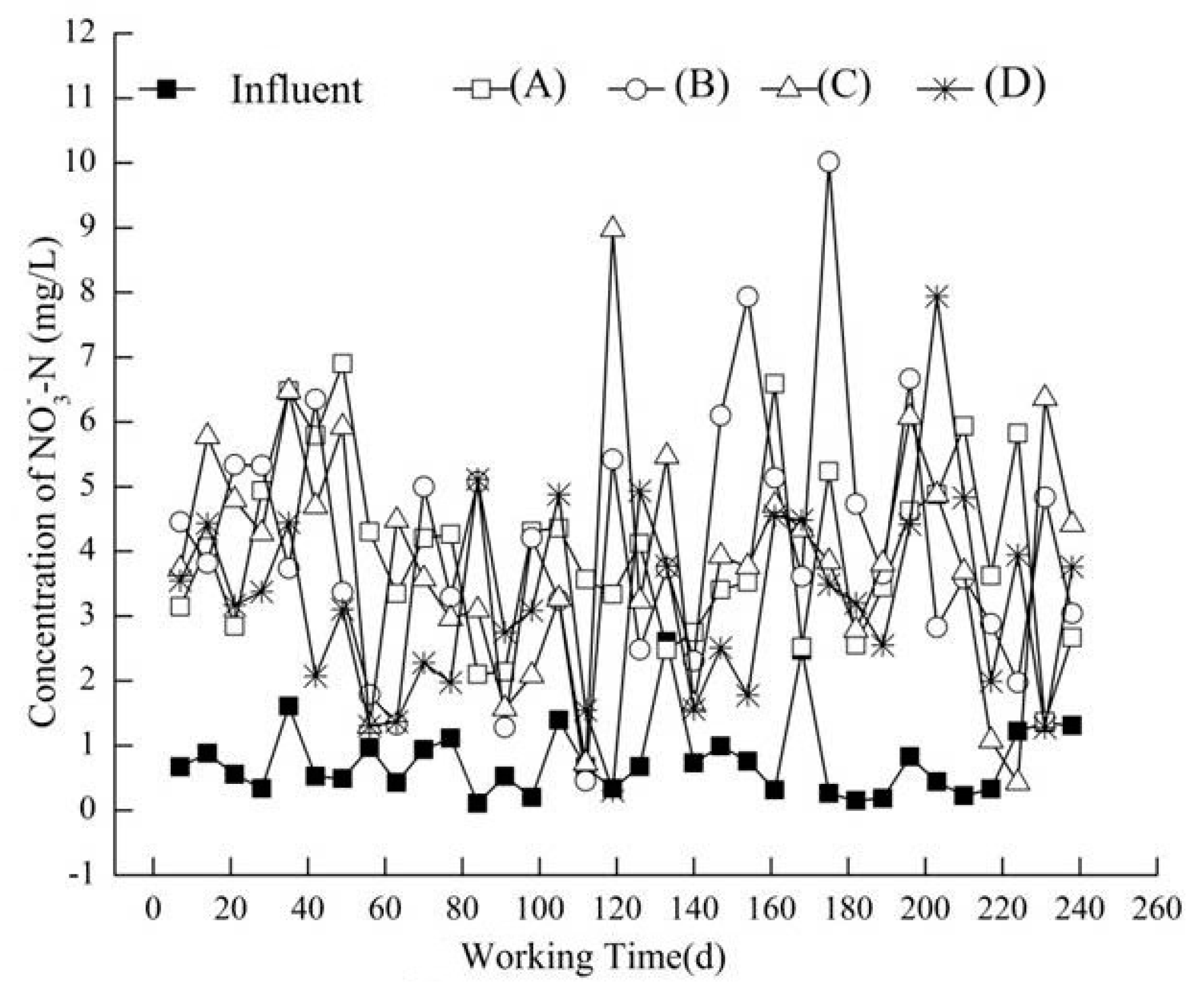
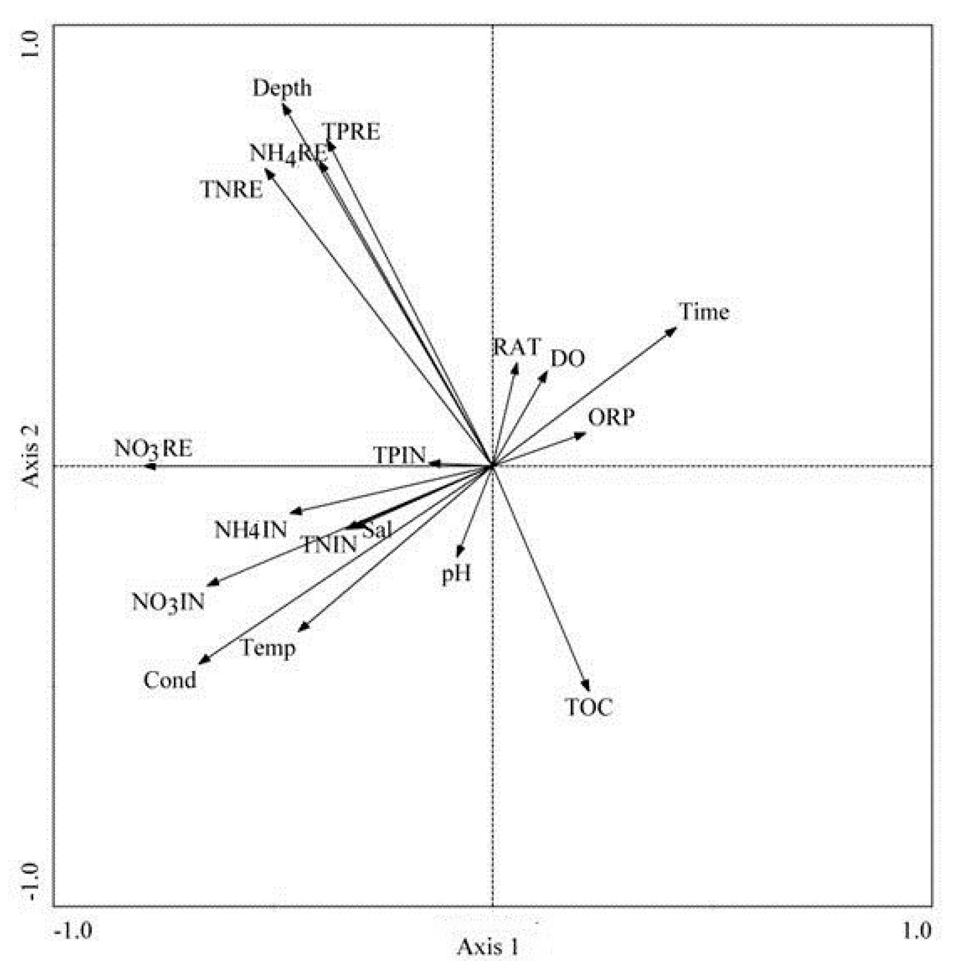
3.1. Nutrient Removal Effect

As shown in Figure 2, the TN removal rates in the four different influent conditions in the TF-CW simulators exceeded 65%, and the mean TN removal rate of the continuous flow simulator was 82 ± 5%. When the idle time/reaction time ratios were 1:1 (B), 1:2 (C), and 2:1 (D), the mean TN removal rates were 85 ± 5%, 86 ± 4%, and 90 ± 3%, respectively (Table 3). The removal was optimal for an idle time/reaction time ratio of 2:1 (D) under tidal flow conditions.
The NH4+-N concentrations in the effluent were statistically significantly lower than those in the influent (Figure 3). The NH4+-N removal rate was higher than 90% and the removal efficiency was greater than that of TN. The removal efficiency of NH4+-N in the tidal flow constructed wetland exceeded 98%, and the NH4+-N removal rates were significantly different between the four influent conditions (p < 0.05) (Table 3).
The NO3-N concentrations in the effluent were higher than those in the influent from the four simulations, mainly because of NO3-N produced during reactions. The removal rates were negative and the difference between the inflow and outflow concentrations in the continuous flow setting was greater than the difference between the inflow and outflow concentrations in the tidal flow simulation devices (Figure 4).
In TF-CWs, TP is mainly absorbed by the matrix. The results in Table 3 show that the TP removal efficiencies of the TF-CW simulator under different influent conditions (A, B, C, D) were 55 ± 14%, 57 ± 16%, 56 ± 19%, and 58 ± 13%, respectively (Figure 5). The TP removal rate did not significantly improve under tidal flow conditions and the natural zeolite did not improve the removal rate of TP from the sewage.

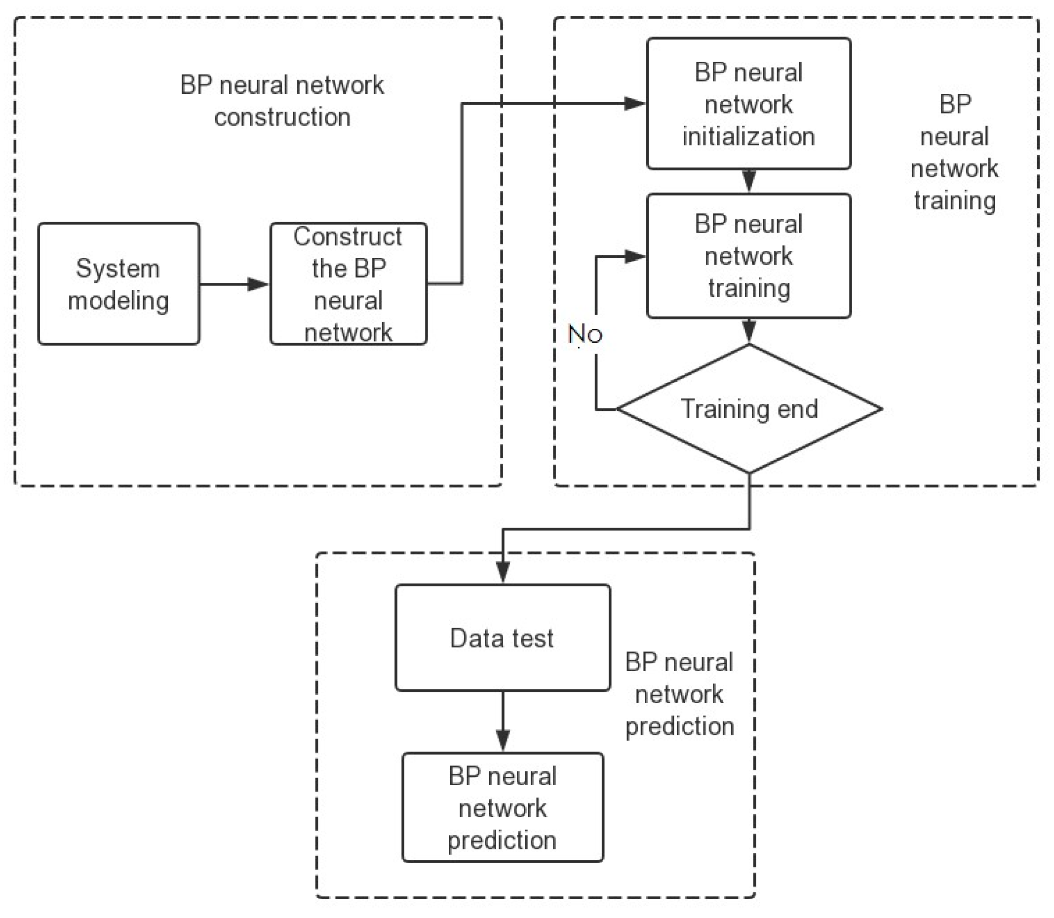
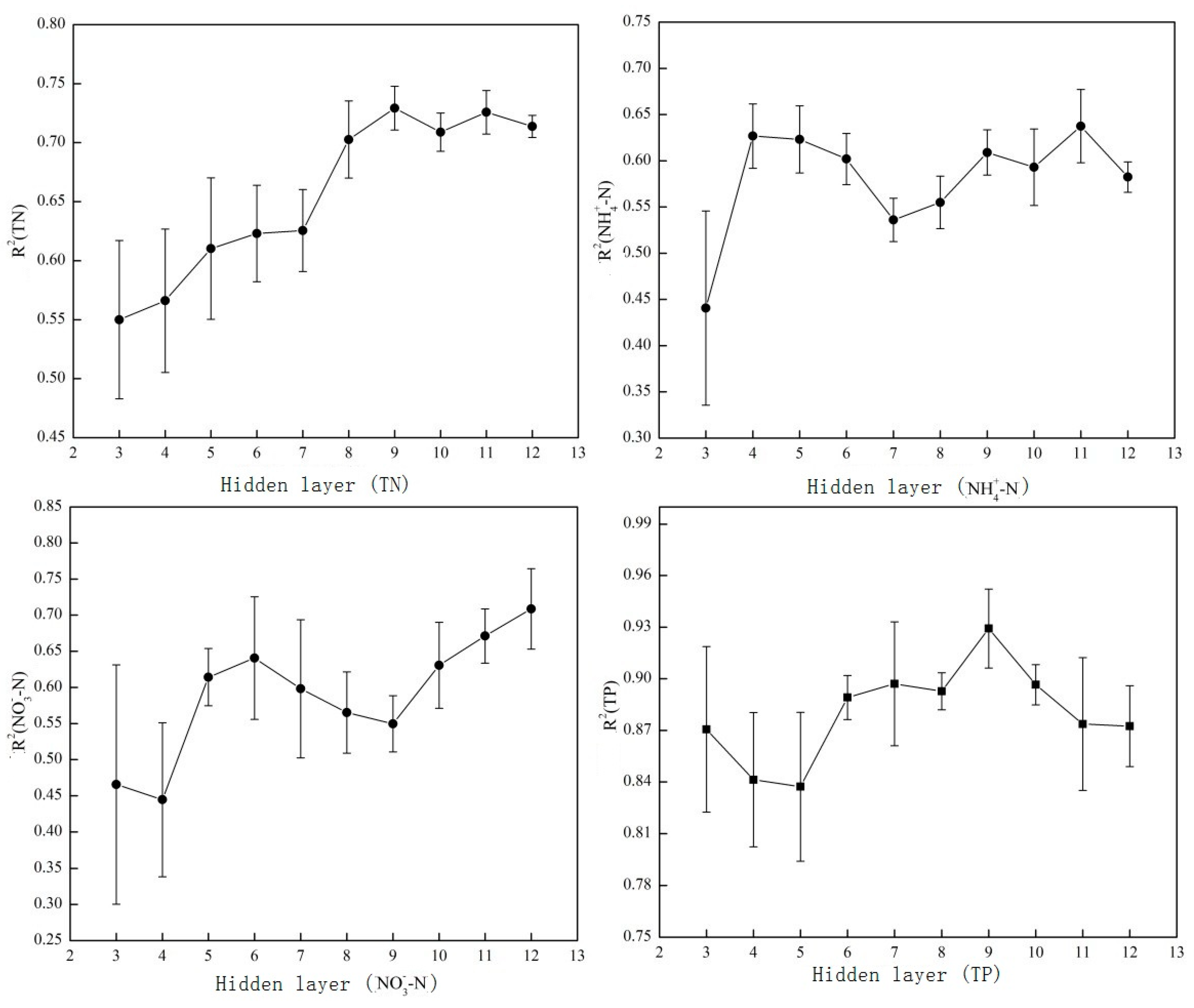
3.2. Building the BP Artificial Neural Network

The development of a nonlinear function fitting algorithm of a BP neural network can be divided into three steps as follows: Construction, training, and prediction [21]. The details of the algorithm flow are shown in Figure 6. This model uses powerful data recognition and simulation capabilities to solve nonlinear system problems. The input and output data are trained on the BP neural network so that the network can express the unknown black box function and then the trained BP neural network can be used to predict the system outputs.
It is difficult to control the basic chemical transformations in ecological engineering applications, and pollutant recycling in wastewater is a highly complicated process. There is considerable variation in the many factors that influence the removal efficiency of different pollutants, and it is impossible to consider the wide range of potential influences as model inputs. In this study, we used redundancy analysis (RDA), based on the actual effluent concentrations, to screen each of the indicators for their influence on the removal efficiency of nutrients in the TF-CW simulator (Figure 7). Redundancy analysis can extract and summarize the variation in a set of response variables that can be explained by a set of explanatory variables. It can also be considered a constrained version of principal components analysis (PCA), where the canonical axes—built from linear combinations of response variables—must also be linear combinations of the explanatory variables [25].
Figure 7 shows that the TN and NH4+-N removal rates were not affected by the operating time, but the removal rate of NO3-N was inversely proportional to the operating time. The removal efficiencies of TN and NH4+-N were stable, but the removal rate of NO3-N decreased gradually. The tidal flow device can effectively purify wastewater with NH4+-N as the main pollutant [26]. The aging rate was slow, and the removal over time was consistent. When RDA was applied to continuous flow, the idle time/emptying time (RAT) value was denoted by 0. The TN and NH4+-N removal rates were positively correlated with RAT.
The NO3-N influent concentration was close to 0, but when coupled with the nitrification of NH4+-N, the NO3-N concentration in the outflow was higher than in the inflow. Therefore, the NO3-N removal rates were negative, but were positively correlated with the NO3-N influent concentrations. Removal rates of NO3-N should be studied in more detail for situations where NO3-N is present at higher concentrations and is the main pollutant. The results from RDA showed that RAT was positively correlated with DO, which indicates that TF-CWs had a higher re-oxygenating capacity than continuous flow constructed wetlands.
The DO concentrations were positively correlated with the TN and NH4+-N removal rates, which shows that DO had a strong influence on the nutrient removal efficiency from wastewater when NH4+-N was the main pollutant [27,28]. Many factors are known to affect NO3-N removal, including pH, conductivity, water temperature, and salinity. When the pH is either too high or too low, it has a large effect on the activity of wetland microorganisms. Temperature affects nitrogen removal by denitrification in constructed wetlands, and the rate decreases when the temperature falls below 5 °C. In contrast to other similar studies [29], the NO3-N removal rate in this study was not significantly correlated with TOC concentrations. The concentrations of TOC in the four devices were low, and thus the correlation between these two parameters was not accurately reflected. The RDA results showed that the NH4+-N removal rates were negatively correlated with the TOC concentrations. In this study, the TOC concentrations (between 0 and 20 mg/L) were too low to provide the energy needed for NO3-N denitrification. Therefore, we need to carry out further studies to examine nitrogen removal in high TOC concentrations and to find a way to maintain the C/N ratio at a level that is conducive to improved nitrogen removal. The TN removal rates were positively correlated with pH, conductivity, water temperature, and salinity; the NH4+-N removal rates were positively correlated with depth, and removals of both TN and NH4+-N were negatively correlated with ORP and TOC (Table 4).
The treatment depth had a major influence on TP removal [30], with a correlation coefficient of 0.65. Other factors did not have major roles, which indicates that substrate adsorption and sedimentation played a leading role in TP removal.
The RDA results indicated that different factors influenced the removals of TN, NH4+-N, and NO3-N. Therefore, we selected different training samples for the different models, as follows: the data collection times were as close as possible to ensure the data were effective, the samples were as diverse as possible, and significant deviations were removed from the actual data because of their influence on the neural network training effect. The model was divided into training data and validation data [31]. The data were divided into 112 groups of training data and 56 sets of validation data using a randomly generated method.
The various indicators of the sample data may not fall within the same order of magnitude, which means that the network cannot converge and thus the time to train the network needs to be increased. To obtain better training results, the index data should be within the same order of magnitude. Before running the model, all the data were mapped to between 0 to 1 and the range of changes of the index were unified, to improve the training efficiency of the network and avoid differences in the order of magnitude that would affect the accuracy of the network recognition. The MATLAB toolbox has many normalization functions, including zscore, premnmx, mapminmax, and postmnmx functions; of these, we used the mapminmax function for the normalization. The output predicted data were the output values of the normalized data, and so the outputs from the network had to be anti-normalized.
x * = x m i n m a x m i n
When the output layer of the model was the TN concentration in the effluent, the input layers were DO, RAT, ORP, and TOC. When the NH4+-N concentration was the output layer, the input layers were DO, RAT, ORP, and Depth. When NO3-N was the output layer, Cond, Temp, Sal, and pH were the input layers. The input layers were DO, RAT, Time, and Depth when the output layer was the TP effluent concentration.
The number of nodes in the hidden layer is very important. The fitting ability of the network improves as the number of nodes in the hidden layer increases. When the number of hidden nodes is small, the network fitting information cannot meet the demand. If the number of hidden layer nodes is infinite, any nonlinear mapping can be implemented from the input to the output. However, the number and training time are positively related. If time is not considered, there may be problem of overfitting, in which an increase in the test error leads to a decrease in the generalization capacity [32]. Therefore, the method used to determine the number of hidden layer nodes is very important, and is a complex problem. It has a certain relationship between the input and output layers, but it does not provide a good formula for deriving this number. In practice, we can combine empirical formulae to calculate the range of hidden layer nodes, and then use the trial and error method to determine the actual number. The empirical formula most commonly used is [32]:
N = n + m + a
where N is the number of hidden layer nodes, n is the number of input layers, m is the number of output layers, and a is a constant (1 to 10). The empirical formula calculation showed that the number of nodes in the hidden layer should be between 3 and 12, and thus the trial-and-error method was then used to train and verify the number of all the network nodes between 3 and 12, and the numbers were tested in the network. The number of nodes was tested 3 to 5 times, and the average coefficient value derived from the 3 to 5 determination coefficients obtained was used as the determination coefficient of the number of nodes. The optimal number of hidden layer nodes was selected from the coefficient.
The relationship between the number of hidden layers and the coefficient of determination (R2) is shown in Figure 8. The coefficient of determination is a non-unit parameter that can directly determine the merits of the fitting indicators. In general, the greater the goodness of fit is, the higher the power of the independent variable to explain the dependent variable [33].
Figure 8 shows that the number of nodes increased as the number of hidden layers increased, and there was a clear increase in the R2 of TN when the number of hidden nodes was 9. The training effect was best when TN had 9 hidden layers. The R2 value reached 0.73 ± 0.02, gradually stabilized, and then decreased slightly. For NH4+-N, when the number of hidden nodes increased from 3 to 4, the training effect improved noticeably, but then the coefficient of the hidden layer started to fluctuate as the hidden layer nodes increased. When the number of hidden nodes reached 11, R2 was maximized and reached 0.63 ± 0.04, which was less than the value for the TN training data. When training the NO3-N data, the effect of the training data increased when the number of nodes in the hidden layer increased. We chose to use 12 hidden layer nodes in the NO3-N network topology, and achieved an R2 of 0.71 ± 0.06. For TP, there was no obvious change as the number of nodes in the hidden layer increased. The overall R2 was high, and reached 0.93 ± 0.02 when the number of hidden nodes was 9. We therefore used 9 hidden layer nodes when predicting the TP effluent concentrations.
Once the input and output layers were determined, the number of nodes in the hidden layer were further selected, and the corresponding topological structure of the artificial neural network model of tidal flow was established. The main influences on TN, NH4+-N, NO3-N, and TP, as indicated by the RDA, were selected as the input layers of the model; there were four input layers and one output layer. Therefore, there were 9, 11, 12, and 9 hidden layer nodes in the input layers of the neural network model, respectively, and one neuron in the output layer.

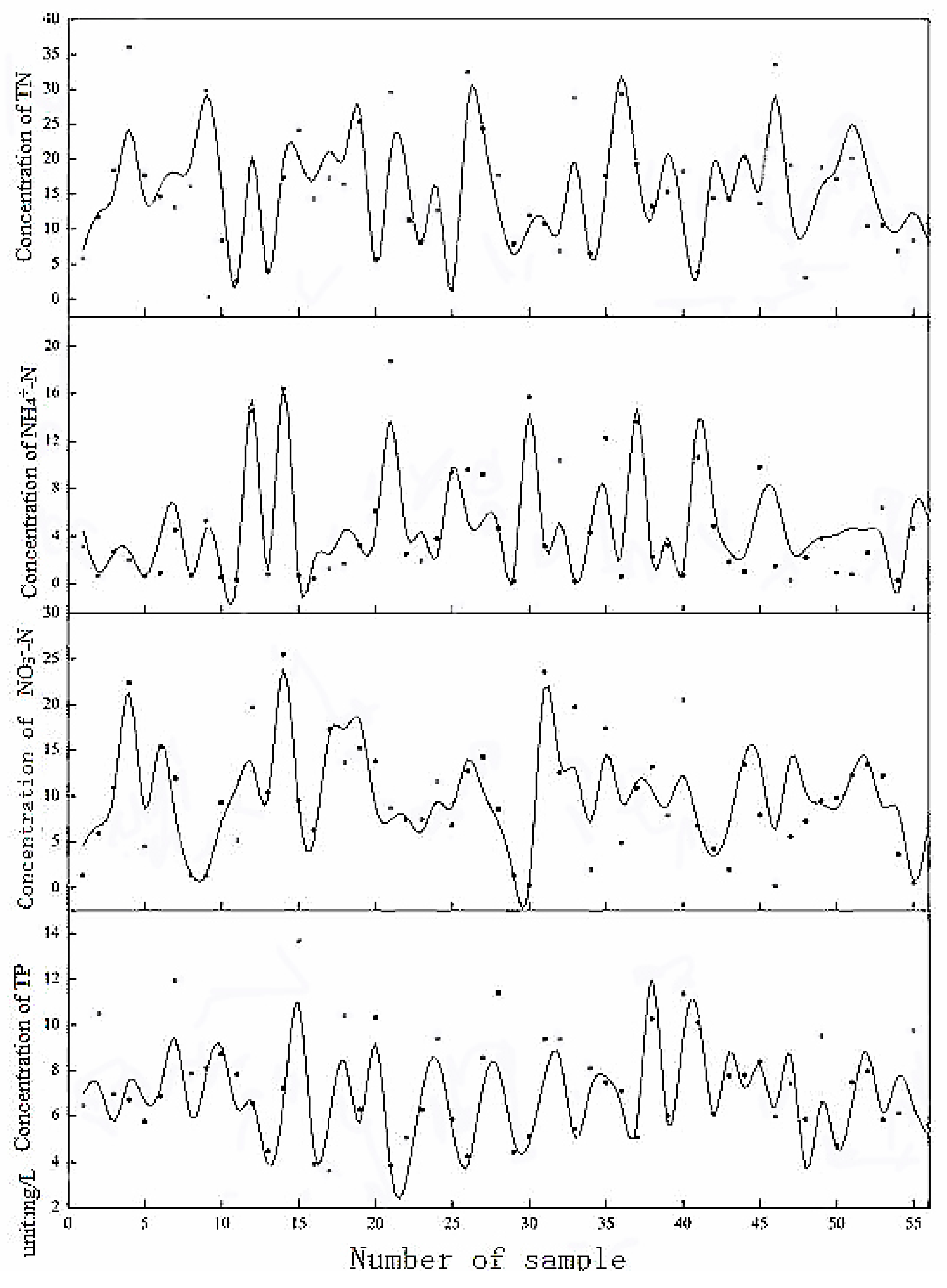
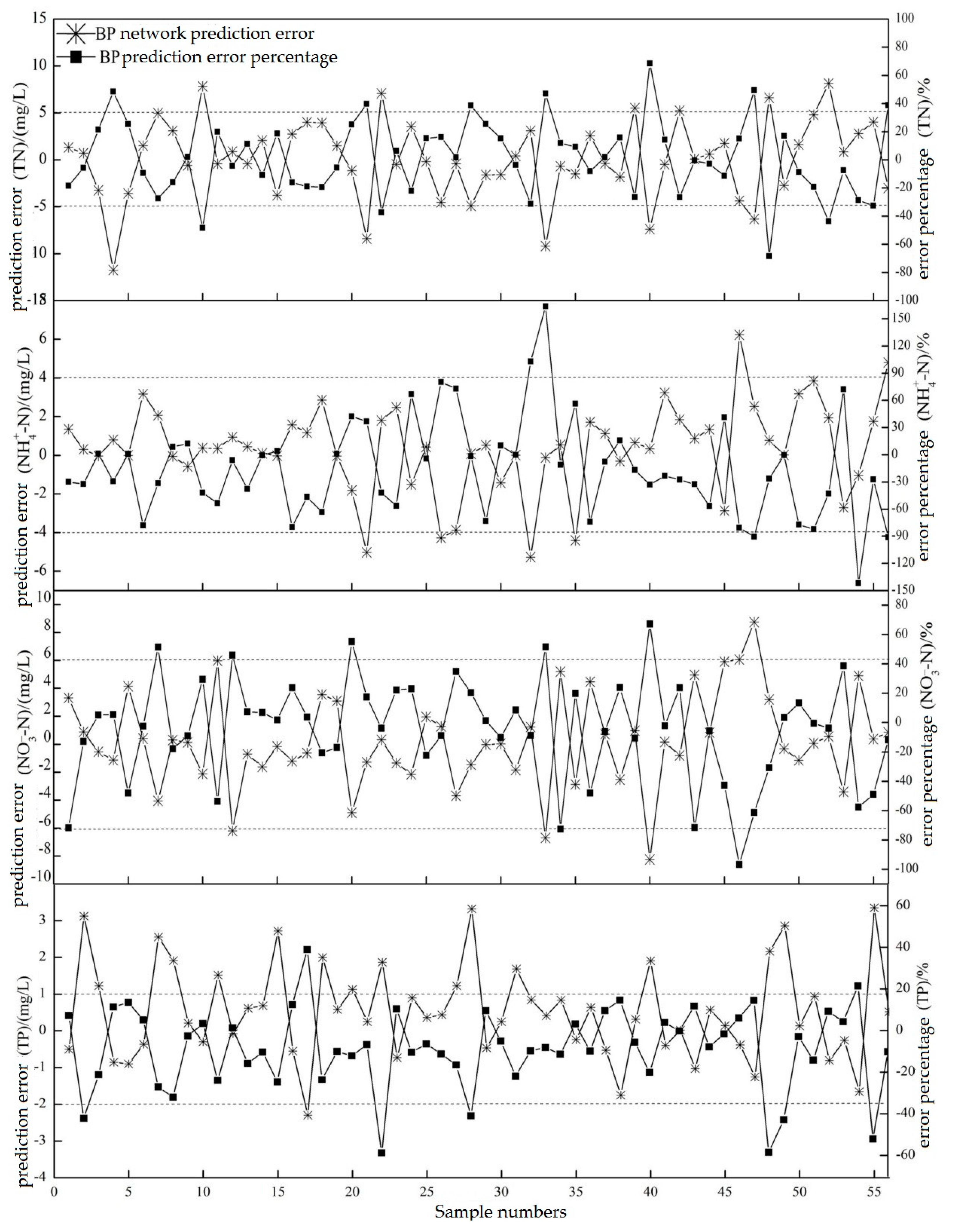
3.3. Comparison of the Predicted and Measured Values

We collected 168 groups of inflow and outflow data, among which we randomly selected 112 sets of data as training samples, and other 56 groups as test samples. The model parameters described in Section 2 were used to train the network. The predicted and measured values are shown in Figure 9.
The results show that the model established by the BP artificial neural network gave reasonable predictions of the nutrient concentrations in the effluent. While there were some errors, some of the predicted and actual values were significantly correlated, and there was minor deviation between the predicted concentrations in the output water and the measured effluent concentrations. The four indicators of the predicted and the measured values showed that there were irregular changes in the concentrations of the output water, mainly because of how the data were arranged. When the training model was used to process data for different treatment depths and different water ways, the data were disrupted and sorted randomly. The first 112 groups were extracted as training data, while the last 56 groups were extracted as the validation data. The data were independent and there were no relationships among them, and thus there were no regular changes in the predicted output water concentrations. When analyzing continuous data, the data should not be sorted randomly with the rand function.

3.4. Training Errors in the BP Neural Network

The prediction error of the BP network and the percentage prediction error are shown in Figure 10.
There were some errors in the effluent concentrations of each index predicted by the BP neural network. The network prediction error percentage and the prediction error fluctuated significantly (p > 0.05). By comparing Figure 9 and Figure 10, we find that, when the measured value was high, the error in the predicted value was very obvious and the prediction percentage error was large; when the measured value was low, the network prediction error and the percentage network prediction error were both low. When there was no functional relationship between the training data and the verification data, the BP neural network had a poor predictive ability, and the network only performed well when the data were regular. The network prediction error in the TN effluent concentrations ranged from −15 to 15 mg/L, and, with 80% of the prediction error between −5 and 5 mg/L, the overall network error was small. The error associated with the predicted NH4+-N effluent concentrations ranged from −8 to 8 mg/L, and 90% of the predicted error was between −4 and 4 mg/L. The obvious variations and the high relative errors resulted from the low effluent concentrations. The errors associated with the predicted NO3-N effluent concentrations were mostly between −6 and 6 mg/L. The results suggest that the BP neural network was better at predicting the effluent concentrations of TP than the other nutrients since the errors associated with the predicted TP concentrations were small and 90% of the TP prediction errors were between −2 and 1 mg/L.

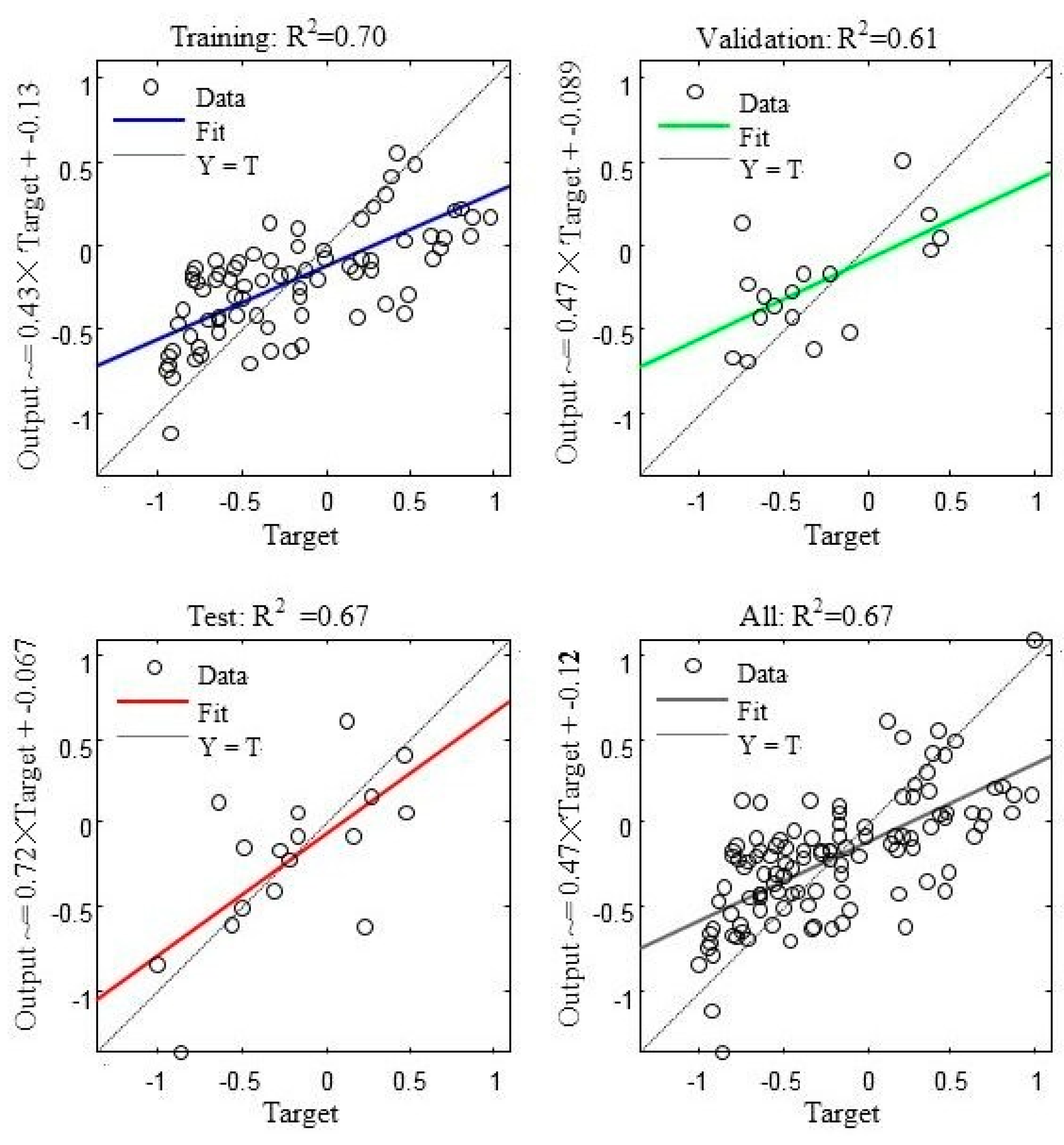
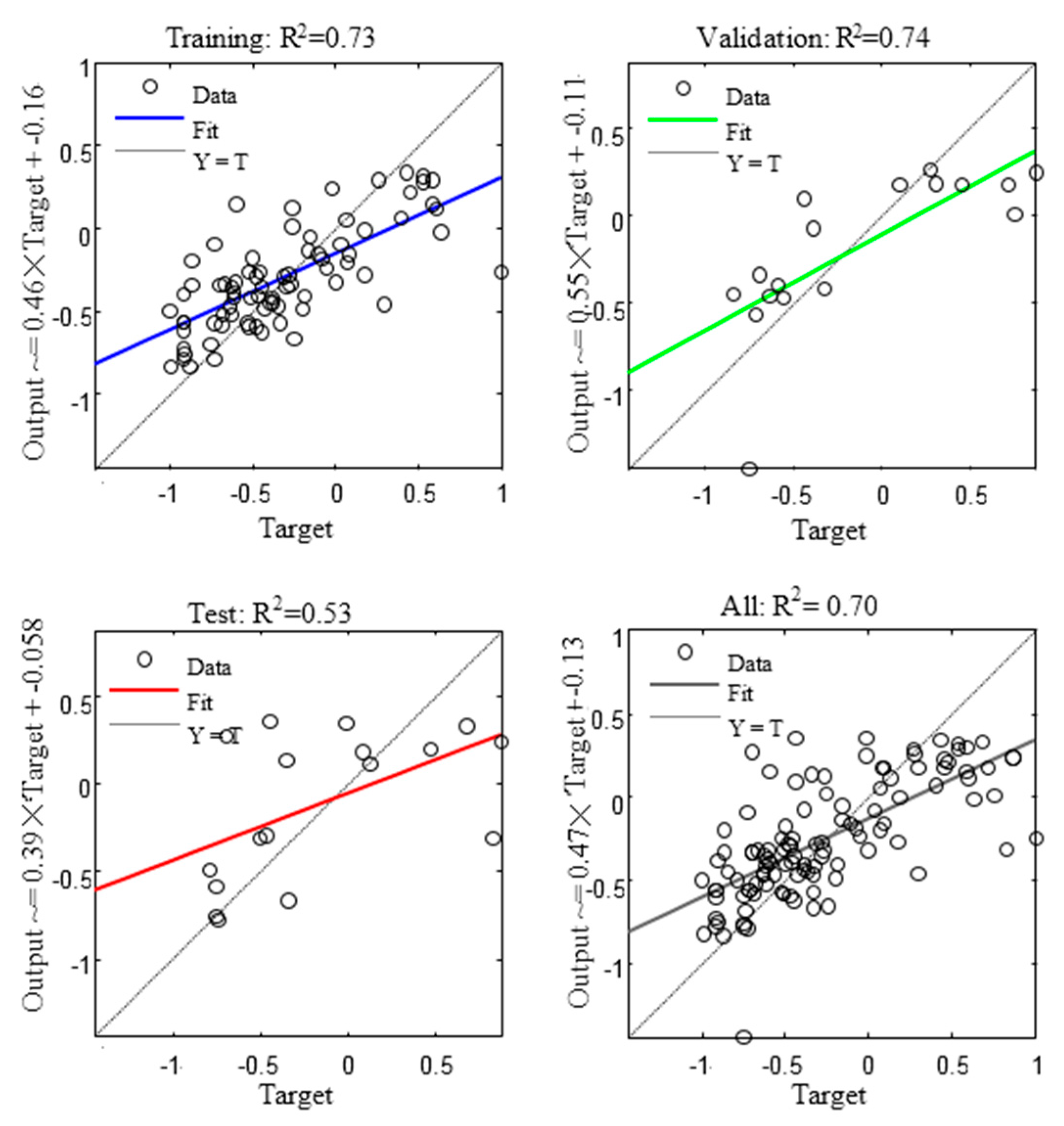
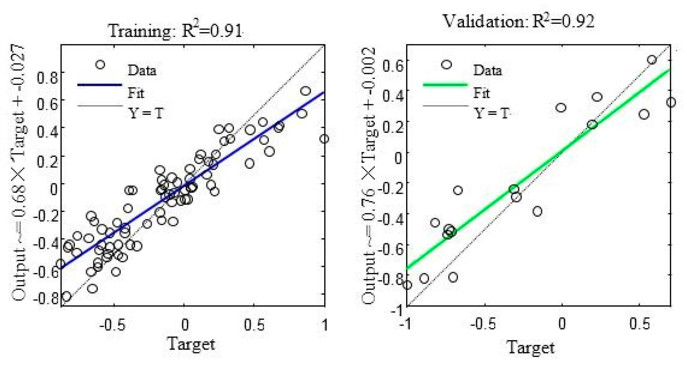
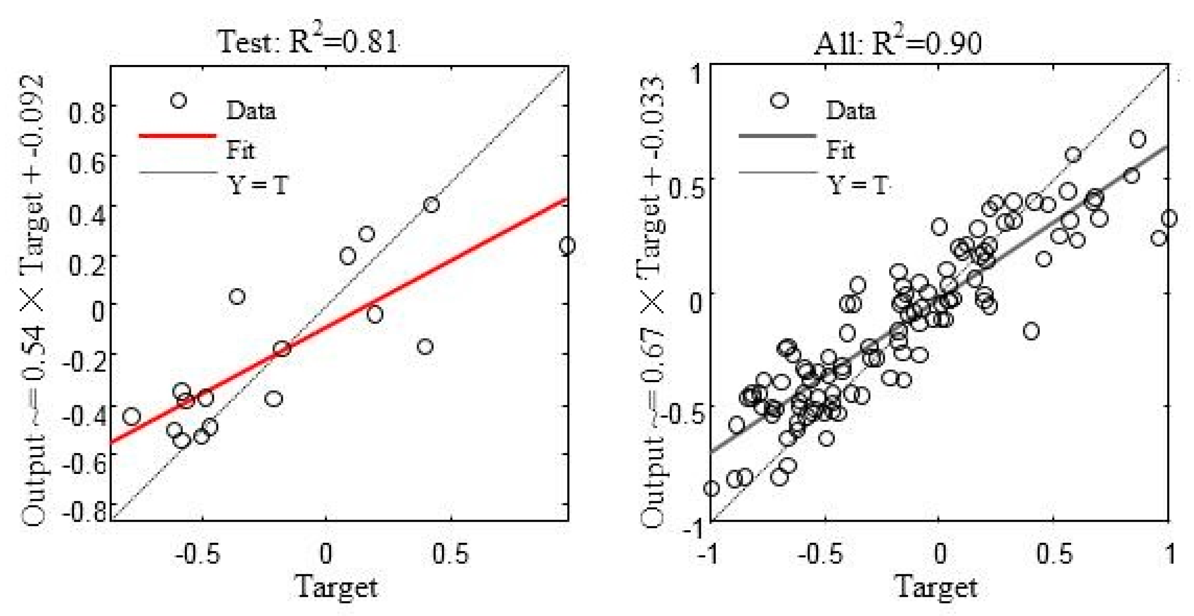
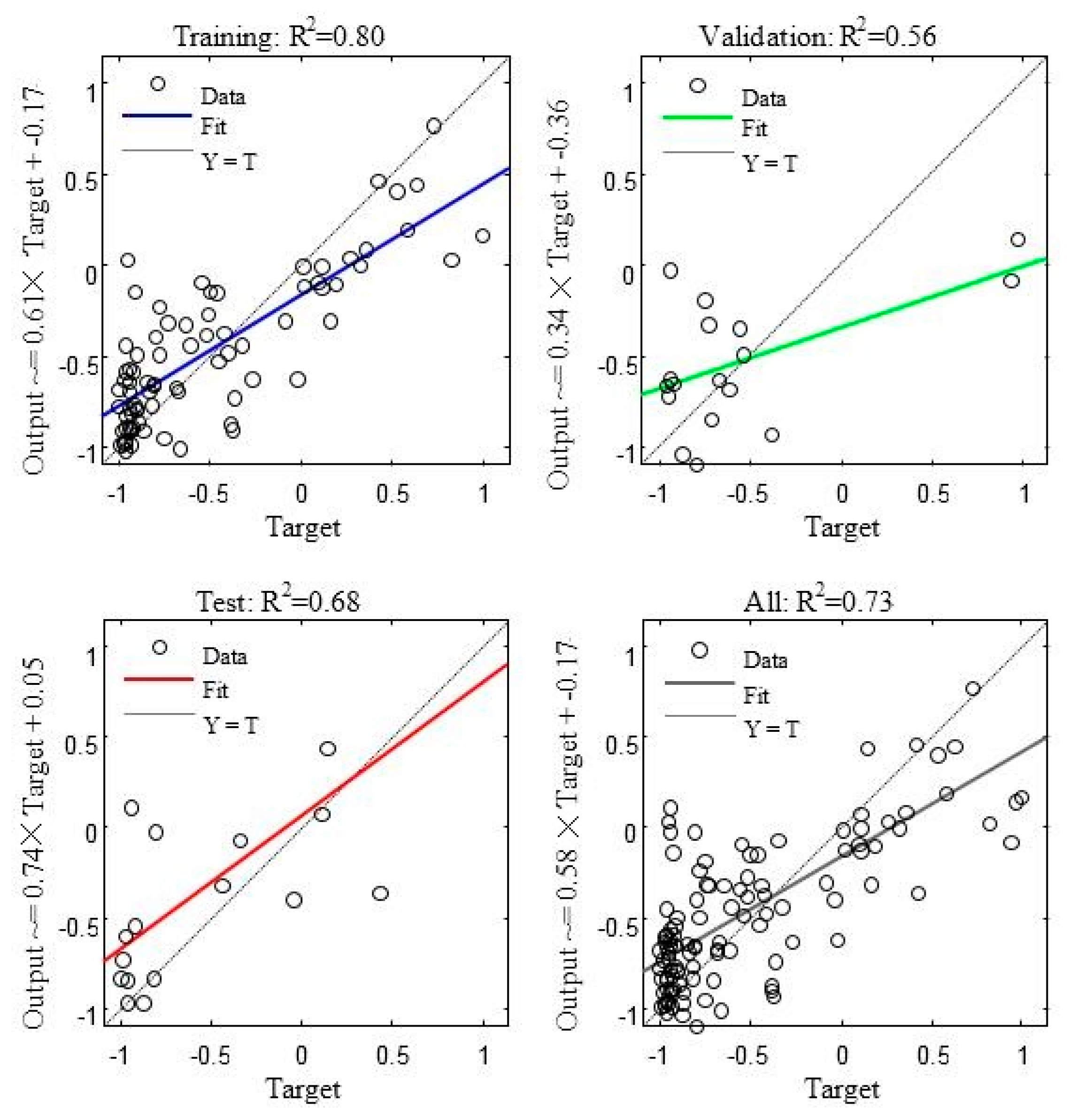
3.5. Network Fitting Ability

The fitting ability of the network is an indication of how well the constructed BP neural network fits to the topological structure. The data were automatically divided into training data, validation data, and test data during the training and prediction. When calculating the fit between the measured and output values of each data, the R2 represented the fitting effect, the fit line represented the fitting curve, Y = T represented the fitted line when R2 = 1, and the degree of fitness decreased as the deviation increased.
The fitting of the BP neural network to the TN effluent concentrations is shown in Figure 11. The R2 value for the training data was 0.70, and the R2 value for the validation data was 0.61. The fitting coefficient of the test data network was 0.67 and the total effect was very good, with an R2 of 0.67.
The fitting of the BP neural network to the NH4+-N effluent concentrations is shown in Figure 12. The R2 values for fitting the training and validation data were 0.80 and 0.56, respectively. The R2 value of the validation data was relatively low because of the lack of data. The fitting coefficient of the test data network was 0.68, and the overall effect was very good with an R2 value of 0.73.
The fitting of the BP neural network to the NO3-N effluent concentrations is shown in Figure 13. The R2 of the training data was 0.73 and, with an R2 of 0.74, fitted well with the validation data. The fitting ability of the test data was poor with an R2 of 0.53. The overall R2 was 0.69.
The above three figures (Figure 11, Figure 12 and Figure 13) show that the quality of the fit of the BP neural network differed for each of the three nitrogen forms. Although there was a large relative error associated with the NH4+-N fitting, it fitted better to the network than the other two nitrogen forms. Therefore, when using BP neural networks, we should not just consider the network error or the percentage network error, but we should also consider the network fitting ability.
The BP neural network fitted well to the TP effluent concentrations (Figure 14). The R2 of the overall fitting ability reached 0.90 and the R2 of the training data was 0.91. The validation data had the best fit with an R2 of 0.92. The overall R2 of the test data was 0.81. The TP concentrations in the effluent were mainly influenced by the Depth, while the effects of the other factors were minimal. Depth was therefore the only input layer of the BP neural network for TP, and the fact that the fitting ability of the TP effluent concentrations was better than that of the other nutrients indicates that networks with only one guiding factor have a better fitting ability and lower error than other networks.

4. Conclusions

In this study, we examined the removal of nutrients in a TF-CW. We used three tidal inflow models and one continuous flow model to examine the removal rate and the variation of each pollutant index at different depths. We used RDA to select the main controls on nutrient removal and applied them as the main factors in the BP neural network for model simulations.
In constructed wetlands, tidal operation can improve the removal rate of nutrients. The tidal flow has a positive effect and refreshes the wetland with fresh air and enhances the dissolved oxygen (DO) in the system. Such intermittent aeration is more effective than continuous aeration, as it facilitates the establishment of aerobic and anaerobic conditions suitable for nitrification and denitrification [34,35]. The different nutrients in these four kinds of water treatment methods behaved differently. The optimal removal efficiency of TN by the tidal flow constructed wetlands was achieved by the influent method with an idle time/reaction time of 2:1 (D), which was significantly different from the other three influent methods (p < 0.05). This treatment also had the optimal NH4+-N intake, which reached 99% ± 1%. The NO3-N concentrations in the effluent from the four simulations were higher than the influent concentrations; the removal rates were negative, and the overall removal efficiency was better in the continuous flow system than in the tidal flow simulation system. The TP removal rates did not differ significantly between the four devices (p > 0.05), and were not significantly higher in the tidal flow system.
Our results show that the ability of the BP artificial neural network model to predict nutrient concentrations in the effluent was good, and there were small errors when correlating the predicted values and the actual values. Of all the indexes, TP had the best fitting ability to the BP neural network, with a total R2 of 0.90. The overall R2 values for TN, NH4+-N, and NO3-N were 0.67, 0.73, and 0.69, respectively. Despite the errors, the BP artificial neural network provides a new method for modeling the effectiveness of TF-CWs. Future studies should explore BP neural networks with multiple hidden layers, and greater generalization abilities and prediction accuracies. For simple mapping, a single hidden layer can be selected to achieve greater speed when the network meets the precision requirements. For complex mapping, the multiple hidden layer can improve the prediction accuracy of the network. We also need to carry out further studies of applications of optimized BP neural networks to TF-CWs based on genetic algorithms.

Acknowledgments

This study was supported by the Fundamental Research Funds for the Central Non-Profit Research Institution of CAF (CAFYBB2014QA029) and “The Lecture and Study Program for Outstanding Scholars from Home and Abroad” (CAFYBB2011007). We thank Alex Boon, PhD, and Deborah Ballantine, PhD, from Liwen Bianji, Edanz Group China (www.liwenbianji.cn/ac), for editing the English text of a draft of this manuscript.

Author Contributions

Wei Li and Lijuan Cui conceived and designed the experiments; Yaqiong Zhang and Xinsheng Zhao performed the experiments; Yaqiong Zhang and Manyin Zhang analyzed the data; Weigang Xu, Xu Pan and Jing Li contributed materials and analysis tools; Yaqiong Zhang, Wei Li, Zhangjie Cai, Yinru Lei, Zhiguo Dou wrote the paper.

Conflicts of Interest

The authors declare no conflict of interest.

References

  1. Behrends, L.; Houke, L.; Bailey, E.; Jansen, P.; Brown, D. Reciprocating constructed wetlands for treating industrial, municipal and agricultural wastewater. Water Sci. Technol. 2001, 44, 399–405. [Google Scholar] [PubMed]
  2. Lee, C.; Fletcher, T.D.; Sun, G. Nitrogen removal in constructed wetland systems. Eng. Life Sci. 2009, 9, 11–22. [Google Scholar] [CrossRef]
  3. Cui, L.J.; Li, W.; Zhang, Y.Q.; Wei, J.M.; Lei, Y.R.; Zhang, M.Y.; Pan, X.; Zhao, X.S.; Li, K.; Ma, W. Nitrogen removal in a horizontal subsurface flow constructed wetland estimated using the first-order kinetic model. Water 2016, 8, 514. [Google Scholar] [CrossRef]
  4. Mitsch, W.J.; Cronk, J.K. Creation and restoration of wetlands: Some design consideration for ecological engineering. Soil Res. 1992, 17, 217–259. [Google Scholar]
  5. Wu, S.; Kuschk, P.; Brix, H.; Vymazal, J.; Dong, R. Development of constructed wetlands in performance intensifications for wastewater treatment: A nitrogen and organic matter targeted review. Water Res. 2014, 57, 40–55. [Google Scholar] [CrossRef] [PubMed]
  6. Zhou, Q.H.; Wang, Y.F.; Wu, Z.B. Progress on study of microorganism in constructed wetlands. Environ. Sci. Technol. 2008, 31, 58–62. [Google Scholar]
  7. Sun, G.; Zhao, Y.; Allen, S. Enhanced removal of organic matter and ammoniacal-nitrogen in a column experiment of tidal flow constructed wetland system. J. Biotechnol. 2005, 115, 189–197. [Google Scholar] [CrossRef] [PubMed]
  8. Zhao, Y.; Sun, G.; Allen, S. Purification capacity of a highly loaded laboratory scale tidal flow reed bed system with effluent recirculation. Sci. Total Environ. 2004, 330, 1–8. [Google Scholar] [CrossRef] [PubMed]
  9. Zhao, Y.; Sun, G.; Lafferty, C.; Allen, S.J. Optimising the performance of a lab-scale tidal flow reed bed system treating agricultural wastewater. Water Sci. Technol. 2004, 50, 65–72. [Google Scholar] [PubMed]
  10. Huang, J.; Reneau, R.B.; Hagedorn, C. Nitrogen removal in constructed wetlands employed to treat domestic wastewater. Water Res. 2000, 34, 2582–2588. [Google Scholar] [CrossRef]
  11. Jing, S.R.; Lin, Y.F. Seasonal effect on ammonia nitrogen removal by constructed wetlands treating polluted river water in southern Taiwan. Environ. Pollut. 2004, 127, 291–301. [Google Scholar] [CrossRef]
  12. Guo, Y.M.; Liu, Y.G.; Zeng, G.M.; Hu, X.J.; Xu, W.H.; Liu, Y.Q. An integrated treatment of domestic wastewater using sequencing batch biofilm reactor combined with vertical flow constructed wetland and its artificial neural network simulation study. Ecol. Eng. 2014, 64, 18–26. [Google Scholar] [CrossRef]
  13. Wang, S.; Zhang, N.; Wu, L.; Wang, Y. Wind speed forecasting based on the hybrid ensemble empirical mode decomposition and GA-BP neural network method. Renew. Energy 2016, 94, 629–636. [Google Scholar] [CrossRef]
  14. Shao, L.M.; Fu, G.; Chao, X.C.; Zhou, J. Application of BP neural network to forecasting typhoon tracks. J. Nat. Disasters 2009, 18, 104–111. [Google Scholar]
  15. Wang, W.; Zhuang, K.; Wu, G.; Zhou, P.; Yang, M.; Li, D.; Jiang, C.; Huang, B. The application of BP neural networks to the new generation expert system for earthquake prediction. Earthquake 1997, 11, 1259–1265. [Google Scholar]
  16. Zhou, Y.; Ruan, R. Application of LM-BP neural networks in remote sensing image classification. Remote Sens. Inf. 2010, 32, 80–86. [Google Scholar]
  17. Li, D.; Wu, G.; Zhao, J.; Niu, W.; Liu, Q. Wireless channel identification algorithm based on feature extraction and BP neural network. J. Inf. Process Syst. 2017, 13, 141–151. [Google Scholar] [CrossRef]
  18. Zhang, Y.; Wu, L. Stock market prediction of S&P 500 via combination of improved BCO approach and BP neural network. Expert Syst. Appl. 2009, 36, 8849–8854. [Google Scholar]
  19. Liu., J.; Jiang, Z.; Wei, J.; Ling, Q. Application of BP neural network model in groundwater quality evaluation. Syst. Eng. Theory Pract. 2000, 20, 124–127. [Google Scholar]
  20. Mo, M.; Wang, X.; Wu, H.; Cai, S.; Zhang, X.; Wang, H. Ecosystem health assessment of Honghu Lake Wetland of China using artificial neural network approach. Chin. Geogr. Sci. 2009, 19, 349–356. [Google Scholar] [CrossRef]
  21. Liang, X.; Chao, F.; Wu, Z.; He, L.; Lu, Y. The application of Neural Network BP to Healthy Assessment of Wetland Ecosystem in Dongting Lake. For. Invent. Plan. 2009, 5, 12. [Google Scholar]
  22. Li, L.; Zhang, H. Assessment model of townlet eco-environmental quality based on BP-artificial neural network. Chin. J. Appl. Ecol. 2008, 19, 2693–2698. [Google Scholar]
  23. Li, R.; Chen, Z.; Chen, Z.; Zhang, X.; Zheng, L.; Wang, Q. Calculation of ecological recovery based on BP neural network: A case study of Zhuxi Small Watershed in Changting County, Fujian Province. Acta Ecol. Sin. 2015, 35, 1973–1981. [Google Scholar]
  24. He, Y.; He, H.; Meng, C.; Xie, M.; Long, M.; Li, Y. Predicting occurrence degree of rice planthoppers in Guangxi Province based on BP artificial neural network method. Chin. J. Ecol. 2014, 33, 159–168. [Google Scholar]
  25. Csala, A.; Voorbraak, F.P.; Zwinderman, A.H.; Hof, M.H. Sparse Redundancy Analysis of High Dimensional Genetic and Genomic Data. Bioinformatics 2017, 33, 3228–3234. [Google Scholar] [CrossRef] [PubMed]
  26. Hu, Y.S.; Zhao, Y.Q.; Zhao, X.H.; Kumar, J.L.G. Comprehensive analysis of step-feeding strategy to enhance biological nitrogen removal in alum sludge-based tidal flow constructed wetlands. Bioresour. Technol. 2012, 111, 27–35. [Google Scholar] [CrossRef] [PubMed]
  27. Saeed, T.; Sun, G. A review on nitrogen and organics removal mechanisms in subsurface flow constructed wetlands: Dependency on environmental parameters, operating conditions and supporting media. J. Environ. Manag. 2012, 112, 429–448. [Google Scholar] [CrossRef] [PubMed]
  28. Wu, S.; Zhang, D.; Austin, D.; Dong, R.; Pang, C. Evaluation of a lab-scale tidal flow constructed wetland performance: Oxygen transfer capacity, organic matter and ammonium removal. Ecol. Eng. 2011, 37, 1789–1795. [Google Scholar] [CrossRef]
  29. Zhi, W.; Ji, G. Quantitative response relationships between nitrogen transformation rates and nitrogen functional genes in a tidal flow constructed wetland under C/N ratio constraints. Water Res. 2014, 64, 32–41. [Google Scholar] [CrossRef] [PubMed]
  30. Vohla, C.; Kõiv, M.; Bavor, H.J.; Chazarenc, F.; Ülo, M. Filter materials for phosphorus removal from wastewater in treatment wetlands—A review. Ecol. Eng. 2011, 37, 70–89. [Google Scholar] [CrossRef]
  31. Li, W.; Zhang, Y.; Cui, L.J.; Zhang, M.Y.; Wang, Y.F. Modeling total phosphorus removal in an aquatic-environment restoring horizontal subsurface flow constructed wetland based on artificial neural networks. Environ. Sci. Pollut. Res. 2015, 22, 12347–12354. [Google Scholar] [CrossRef] [PubMed]
  32. Shen, H.; Wang, Z.X. Determining the number of BP neural network hidden layer units. J. Tianjin Univ. Tech. 2008, 24, 13–17. [Google Scholar]
  33. Zhang, J. Study on Coefficient of Correlation as Goodness-of-fit Criterion. J. Zhengzhou Univ. Technol. Nat. Sci. Ed. 2001, 22, 72–74. [Google Scholar]
  34. Kizito, S.; Lv, T.; Wu, S.; Ajmal, Z.; Luo, H.; Dong, R. Treatment of anaerobic digested effluent in biochar-packed vertical flow constructed wetland columns: Role of media and tidal operation. Sci. Total Environ. 2017, 592, 197–205. [Google Scholar] [CrossRef] [PubMed]
  35. Ilyas, H.; Masih, I. The performance of the intensified constructed wetlands for organic matter and nitrogen removal: A review. J. Environ. Manag. 2017, 198, 372–383. [Google Scholar] [CrossRef] [PubMed]
Figure 1. Experimental tidal flow constructed wetland (TF-CW) setup.
Water 10 00083 g001
Figure 2. Removal rates of total nitrogen (TN) in the four different devices (A–D).
Water 10 00083 g002
Figure 3. Removal rate of NH4+-N in the four different devices (A–D).
Water 10 00083 g003
Figure 4. NO3-N removal rates in the four different devices (A–D).
Water 10 00083 g004
Figure 5. Total phosphorus (TP) removal rates in the four different devices (A–D).
Water 10 00083 g005
Figure 6. Backpropagation (BP) neural network algorithm process.
Water 10 00083 g006
Figure 7. RDA ordinations for various environmental factors in the TF-CW simulator. Note: TNRE: TN removal rate; NH4RE: NH4+-N removal rate; NO3RE: NO3-N removal rate; TPRE: TP removal rate; TNIN: TN influent concentration; NH4IN: NH4+-N influent concentration; NO3IN: NO3-N influent concentration; TPIN: TP influent concentration; TOC: total organic carbon; ORP: oxidation–reduction potential; Time: operation hours; RAT: idle time/emptying time; DO: dissolved oxygen; Sal: salinity; Cond: conductivity; Temp: water temperature; Depth: depth of treatment.
Water 10 00083 g007
Figure 8. Relationship between the coefficients of determination (R2) and the number of hidden layers.
Water 10 00083 g008
Figure 9. Fitting curve values and model output values.
Water 10 00083 g009
Figure 10. Prediction error and the percentage prediction error of the BP network.
Water 10 00083 g010
Figure 11. Fitting of the BP neural network to the TN effluent concentrations.
Water 10 00083 g011
Figure 12. Fitting of the BP neural network to the NH4+-N effluent concentrations.
Water 10 00083 g012
Figure 13. Fitting of the BP neural network to the NO3-N effluent concentrations.
Water 10 00083 g013
Figure 14. Fitting of the BP neural network to the TP effluent concentrations.
Water 10 00083 g014aWater 10 00083 g014b
Table 1. Water quality of influent wastewater.
Indexρ/(mg/L)pH
TNNH4+-NNO3-NTOCTP
Range30~5030~500~50~2010~167~9
Table 2. Time settings of the different water inputs to the TF-CW simulator.
NumberInflow ModeIdle Time (h)Reaction Time (h)Idle/Reaction Time
AContinue flow
BTidal flow12121:1
CTidal flow8161:2
DTidal flow1682:1
Note: The idle time is the time used to inject water into the equipment. The reaction time indicates the time for the biochemical reaction to occur in the wetland.
Table 3. Removal efficiency of nutrients in the different TF-CW simulators.
Inflow ModeTN Removal Rate(%)NH4+-N Removal Rate (%)TP Removal Rate (%)
A82 ± 5 a95 ± 3 a55 ± 14 a
B85 ± 5 b98 ± 1 b57 ± 16 a
C86 ± 4 b99 ± 1 b56 ± 19 a
D90 ± 3 c99 ± 1 c58 ± 13 a
Note: Differences between a, b, and c indicate significant differences at the 0.05 level, the average ± standard deviation.
Table 4. Correlation coefficient matrix.
IndexNO3RENH4RETNRETPRENO3INNH4INTNINTPINTOCRATDOTempCondSalpHORPTimeDepth
NO3RE
NH4RE0.18
TNRE−0.030.06
TPRE−0.29−0.17−0.02
NO3IN0.52−0.24−0.360.11
NH4IN−0.37−0.10−0.250.050.75
TNIN−0.27−0.13−0.120.040.630.87
TPIN0.120.01−0.670.080.350.290.04
TOC0.07−0.35−0.300.03−0.17−0.280.240.32
RAT0.040.20.120.190.000.000.000.000.16
DO0.100.190.100.250.01−0.020.020.010.100.92
Temp0.25−0.33−0.180.150.650.740.470.470.180.050.04
Cond0.33−0.30−0.270.100.750.610.390.470.130.160.160.76
Sal0.35−0.13−0.120.010.170.030.110.320.060.110.130.200.52
pH0.46−0.18−0.260.12−0.45−0.540.530.350.390.060.070.270.140.12
ORP−0.37−0.47−0.420.070.070.010.050.070.070.180.220.120.210.15−0.15
Time−0.530.18−0.180.18−0.030.300.400.130.150.000.040.160.300.29−0.520.32
Depth−0.380.430.040.650.000.000.000.000.560.000.060.220.110.04−0.13−0.100.00

