Ecosystem Services Mapping Uncertainty Assessment: A Case Study in the Fitzroy Basin Mining Region


1
Environment Centres, Sustainable Minerals Institute, The University of Queensland, Brisbane 4072, Australia
2
School of Environmental and Geographical Sciences, The University of Nottingham Malaysia Campus, Kuala Lumpur 43500, Malaysia
*
Author to whom correspondence should be addressed.
Water 2018, 10(1), 88; https://doi.org/10.3390/w10010088
Submission received: 23 November 2017
/
Revised: 8 January 2018
/
Accepted: 10 January 2018
/
Published: 19 January 2018
(This article belongs to the Special Issue Water Stewardship in Mining Regions)
Abstract
:Ecosystem services mapping is becoming increasingly popular through the use of various readily available mapping tools, however, uncertainties in assessment outputs are commonly ignored. Uncertainties from different sources have the potential to lower the accuracy of mapping outputs and reduce their reliability for decision-making. Using a case study in an Australian mining region, this paper assessed the impact of uncertainties on the modelling of the hydrological ecosystem service, water provision. Three types of uncertainty were modelled using multiple uncertainty scenarios: (1) spatial data sources; (2) modelling scales (temporal and spatial) and (3) parameterization and model selection. We found that the mapping scales can induce significant changes to the spatial pattern of outputs and annual totals of water provision. In addition, differences in parameterization using differing sources from the literature also led to obvious differences in base flow. However, the impact of each uncertainty associated with differences in spatial data sources were not so great. The results of this study demonstrate the importance of uncertainty assessment and highlight that any conclusions drawn from ecosystem services mapping, such as the impacts of mining, are likely to also be a property of the uncertainty in ecosystem services mapping methods.
1. Introduction
Ecosystem services (ES) are the benefits that ecosystems provide to human beings, bridging the connection between ecological and social systems [1,2,3,4]. This concept is increasingly used in both theoretical and applied research [5,6] such as spatial planning [7,8], environmental economics [9] and risk management [10]. ES play a crucial role for supporting ecosystem-based management and decisions [11,12] and the mismanagement of ES can potentially have large economic impacts and may affect thousands of people [13,14]. In order to support the decision-making, accurate and reliable methods and outputs for ecosystem services assessments are increasingly demanded [15,16].
Among the various ecosystem services assessment methods, ecosystem services mapping has received increasing attention [17,18]. Mapping is a significant tool for identifying and quantifying the spatial characteristics of ecosystem services [19]. Mapping can provide researchers and decision makers with spatially explicit information to help make feasible policies and strategies [20,21]. There has been a growing number of publications on ES mapping including significant reviews [17,18,22,23] and case study applications from different perspectives and scales [24,25]. A range of mapping methods and integrated mapping tools have been developed, such as the widely used InVEST (Integrated Valuation of Ecosystem Services and Trade-offs) [26] and ARIES (Artificial Intelligence for Ecosystem Services) [27]. Furthermore, a growing number of ES mapping research groups and projects have been established by different research organizations and governments, such as the Ecosystem Services Partnership and Natural Capital Project [19].
Although the number of ES mapping studies has increased, there are still multiple challenges due to models’ limitations, data availability and other relevant issues [17,28]. For instance, different mapping methods may produce completely different outputs for the same ecosystem service [29,30], while data availability may limit the choice of mapping methods and affect map accuracy [31,32]. Consequently, there are many uncertainties in ecosystem services mapping, which are complicated and expressed in different ways. These uncertainties make accurately assessing and explicitly conveying ecosystem services values and spatial distributions for researchers and decision-makers challenging. A crucial step forward is conducting an assessment of uncertainty to quantify the robustness and reliability of a study, test key hypotheses and identify hedging opportunities [33].
Although it is recognized that uncertainties are significant for ecosystem services mapping and modelling, only a small fraction of the literature has assessed uncertainty and only a few studies have focused specifically on uncertainty [16,33,34,35,36]. This contrasts with the literature for other spatially explicit modelling in related disciplines such as landscape ecology and hydrology [37,38,39,40,41]. However, the assessment of uncertainty in ES mapping is growing and there are various definitions and perspectives used in analysing uncertainties [16,33,35,36].
Existing studies on uncertainty and uncertainties derivations in ES assessment generally consider three types of uncertainty [33,35]. Firstly, there are uncertainties associated with characterizing ecological functions and processes. Ecosystem functions are complicated and for many mechanisms there is still not a clear and sufficient understanding [20,42]. Secondly, uncertainties arise from subjective preferences of researchers and other participants. For instance, as the purpose of ES modelling may vary from theoretical predictions, making practical decisions or communication with stakeholders, the preferences of researchers for a specific model and parameterization will result in different forms of uncertainty [43,44]. Also differences in expert experience or the subjective judgments about relative ecosystem services can lead to uncertainties [45,46]. Finally, practical uncertainty may result from the modelling process employed such as the modelling methods and data. Differences between diverse modelling methods used for the same ecosystem service may lead to differences in outputs [35].
The objective of this study was to assess the impact of uncertainty on ecosystem services mapping. We used the Fitzroy Basin mining region as a case study to map hydrological ecosystem service water provision with InVEST. Uncertainty was modelled by altering various inputs and parameterizations of the ES model. A baseline was constructed using the best available data and parameterization using the seasonal water yield model of InVEST. We then assessed three types of uncertainty: (1) spatial data sources, (2) modelling scales (temporal and spatial) and (3) parameterization and model selection. We compared outputs from the baseline model to the uncertainty scenarios using a range of indices. We conclude by discussing the implications of uncertainty for ecosystem services mapping and potential for future research on ecosystem services mapping uncertainty.
2. Materials and Methods
2.1. Study Area
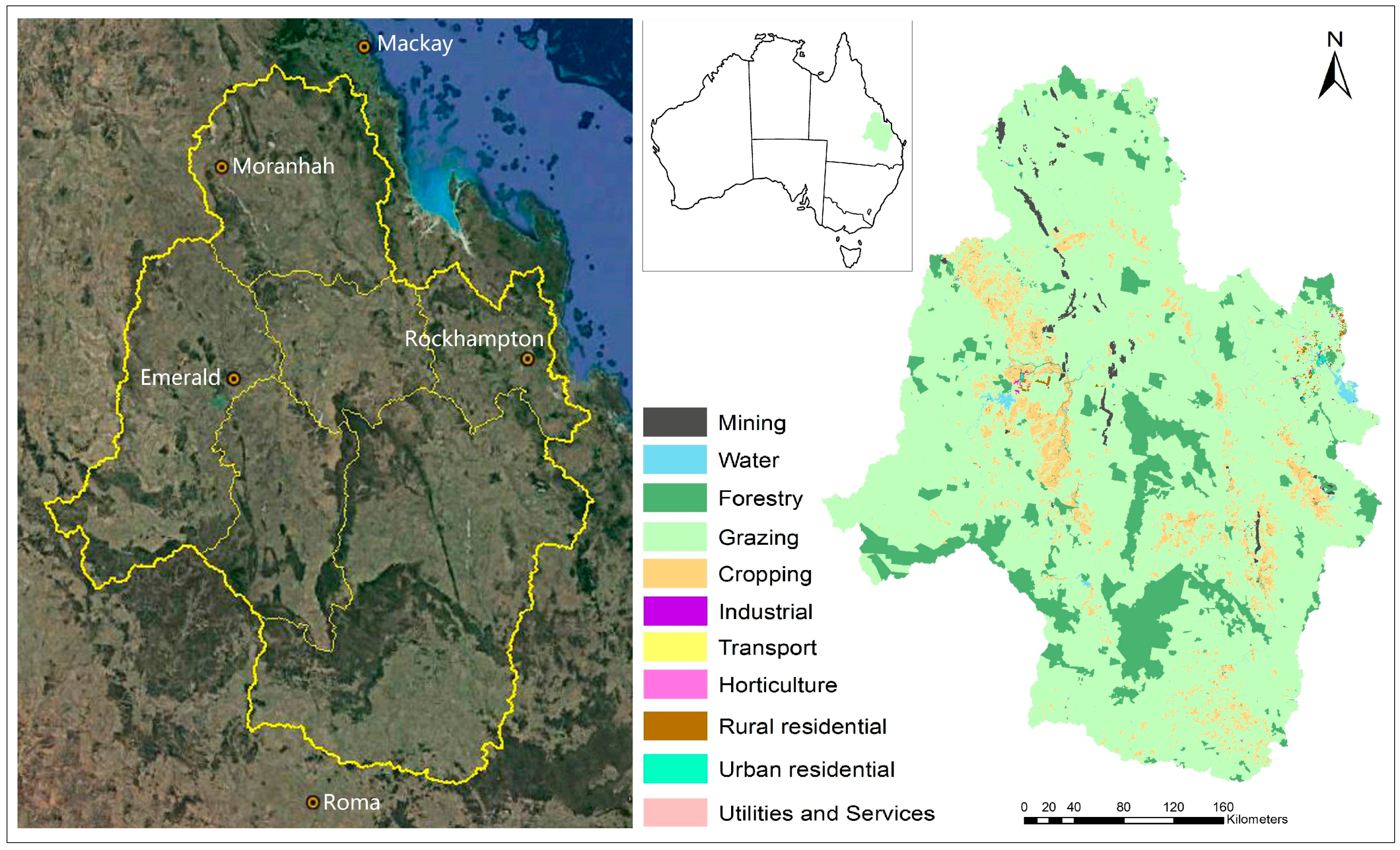
The study area was the Fitzroy Basin (Figure 1), one of the largest (142,665 km²) basins in the Great Barrier Reef catchments and also one of the largest region in Australia [47]. There are six sub-catchments drained by six rivers including the Isaac-Connors, Mackenzie, Comet, Nogoa, Fitzroy and Dawson rivers. The region has a dry and wet season with distinctive climatic characteristics and the mean rainfall for the basin is approximately 630 mm (1920–2005). Most of the study area is relatively flat except the north-eastern area with low hills. The main land uses are grazing, cropping and forest, as well as mining. The urban and towns mainly service the coal mining industry and agriculture [48]. The Fitzroy Basin catchment is of great strategic significance; both environmental and economic [49,50]. On one hand, minerals production provides enormous economic stimuli for the industry and for local community development. On the other hand, the environmental and ecological protection have attracted more and more attention from researchers and public, especially concerns associated with hydrology such as water supply and water quality and the impacts on Australia’s Great Barrier Reef World Heritage Marine Park.
2.2. Baseline Scenario and Ecosystem Service Models
This study focused on the hydrological ecosystem service—water provision—characterized by water yield at both the pixel and catchment scales. We set a Baseline scenario based on the InVEST seasonal water yield model to characterize the water provision service of the study area. This scenario was used as reference which was based on the most feasible ES model with the best available data, precise ES model and appropriate parameterization for local conditions. For example, the seasonal water yield model was used rather than an annual model as it can better reflect the real climate conditions caused by the distinctive wet and dry season of the study area as opposed to an annual water yield model which is also commonly used. The uncertainty scenarios represent realistic alternative ways of modelling ES for the study area.
2.2.1. Seasonal Water Yield Model
The seasonal water yield model in InVEST is a spatially explicit raster based method for characterizing water yield based on three outputs: quick flow, local recharge and base flow. Quick flow characterizes short term stream flow generated from storm rainfall [51], which is calculated based on the runoff curve number method, developed by USDA (United States Department of Agriculture) Natural Resources Conservation Service (the runoff curve number predicts runoff or infiltration from excess rainfall for classified hydrological soil groups). Base flow characterizes stream flow emanating from groundwater. Finally, local recharge is water which moves from the surface to recharge groundwater, which in turn can contribute to potential base flow. Details of the model processes can be found in Table 1 [26,52,53].
2.2.2. Data Sources and Processing
The inputs for the Baseline scenario using the seasonal water yield model include spatial GIS layers and biophysical parameters. Among the spatial layers, monthly precipitation and reference evapotranspiration were provided by the climate database of Australian Bureau of Meteorology [26]. The Digital Elevation Model (DEM) layer was derived from the SRTM-derived 3 Second Digital Elevation Model Version 1.0 [54], which provides better quality and consistency compared to the original SRTM data [55]. Four hydrologic soil groups (HSG A, B, C and D) were classified based on the CSIRO dataset of saturated hydraulic conductivity [56] for assessing infiltration capability of different soil, which represent low to high runoff potential from HSG A to D. The values for the Land use land cover (LULC) were reclassified from the QLUMP (Queensland Land Use Mapping Program) land use classification maps [57]. The QLUMP land use mapping methodology integrated satellite images together with field survey and local expert knowledge and provides the most reliable and accurate LULC for the region. We reclassified the mined land area based on a previous research [58,59] into four types including bare land, industrial, grazing and water, where the biophysical parameters were the same as the QLUMP classifications (Table 2). All the spatial layers were processed in ArcGIS [60] and resampled to the same resolution of 90 m based on a majority for the categorical data and average values for the quantitative data.
The parameters, runoff curve number, monthly rain events, threshold flow accumulation and crop factor Kc values were derived from a range of sources including previous studies and weather station data. The curve number is related to land use and soil attributes such as soil type and infiltration capability [61]. The runoff curve numbers (Table 2) were determined by an Australian developed hydrological software CatchmentSIM [62] and related literature [63,64]. The monthly rain events values were the numbers of rain events higher than 0.1 mm [26], which were derived from the long term weather station observation data in the study area [65]. The threshold flow accumulation is the number of upstream cells that must flow into a cell before it is considered part of a stream, used to classify streams in the model. According to the InVEST handbook [26], previous local research [66] and the stream network dataset from local government [67], we assumed a flow contribution area of 1 km2. The monthly Kc (Table A1, Appendix A) were calculated from remote sensing data of fPAR (fraction of Photosynthetically Active Radiation). The calculation method uses the following equations [26,68,69,70,71], where FC is the Fraction Cover and LAI describes the Leaf Area Index (Equation (1)). The fPAR data was extracted from the Australia fPAR dataset version 5 [72].
2.3. Uncertainty Assessment Overview
Besides the Baseline scenario, six uncertainty scenarios were developed, where a single input for the ES model was altered for each scenario (Table 3). The alternative uncertainty scenarios represent reasonable input parameterizations or modelling methods, however, less precise and/or with greater uncertainty. For example, they might represent the type of data that might be used in data poor regions. Through the six uncertainty scenarios, we assessed three types of uncertainty including: (1) spatial data sources, (2) modelling scales (temporal and spatial) and (3) parameterization and model selection.
2.4. Uncertainty Scenarios
2.4.1. Digital Elevation Model (DEM)
This scenario utilized a DEM layer derived from 1:100,000 contours map sheets surveyed by the AUSLIG (Australian Surveying and Land Information Group) [73]. Topography is the key factor for determining stream networks and other hydrological characteristics of a catchment [74,75]. The scenario aimed to characterize uncertainties caused by different data sources and data precision. This source is different to the SRTM derived DEM used in the baseline as it is less precise and has a coarser map scale than the baseline. In addition, it only delineated the original natural topography for the whole basin and does not include anthropogenic changes such as those associated with mining disturbance.
2.4.2. Land Cover Map
This scenario aimed to assess the uncertainties associated with land use and land cover classification system mapping. For this scenario the National Dynamic Land Cover (NDLC) [76] was used instead of QLUMP. The NDLC Land cover was reclassified for the modelling of ecosystem services to fifteen land cover types (Table 2). The NDLC dataset is a national-scale land cover dataset for Australia, produced by Geoscience Australia and the Australian Bureau of Agriculture and Resource Economics and Sciences. Compared with the QLUMP map used in the baseline, there are a greater number of detailed vegetation cover classifications, which are useful to identify changes in vegetation cover and extent, however, as it is a national scale map it is less accurate thematically and spatially. The Kc values for each land cover (Table A2, Appendix A) and the other parameters were calculated using the same methods as the Baseline scenario.
2.4.3. Climate Data Temporal Scale
This scenario substitutes monthly data for precipitation and evapotranspiration with annual data to assess the impact of the temporal scale of the climate data. Under this scenario, we still utilized the seasonal water yield model but assumed that only annual climate data were available. It is common for water yield modelling to be based on annual data. But for areas where the climate conditions have distinctive seasons, using annual data and models may provide inaccurate assessment of water yield. For example, high intensity rainfall over short periods can saturate soils resulting in greater overland flow and less infiltration than the same amount of rainfall over longer periods.
The monthly inputs into the seasonal water yield model were calculated by dividing annual data into twelve equal values. This scenario is similar to the Annual model scenario in that it considers only annual climate data, however, the annual model uses a different method for modelling water yields and includes different input data i.e. plant available water fraction and root depth. Thus, we could assess differences associated with ignoring seasonal variability without the assessment being confounded by using a different model with different inputs.
2.4.4. Spatial Scale
This scenario tested the impact of spatial scale by resampling all the baseline data by 10. This scenario aimed to assess the impact of spatial scale on ecosystem services mapping and modelling. Assessing spatial scale-dependencies of spatially explicit phenomena is one of the central questions in landscape ecology and geographic research [77,78].
2.4.5. Annual Model
The annual water yield model was applied in this scenario instead of the seasonal water yield model. As described above in Section 2.4.3, it is common for water yield modelling to use only annual data. In fact, earlier versions of InVEST (i.e., version 3.2.0) only included the annual water yield model. The annual water yield model is based on the Budyko curve and annual average precipitation. The Budyko curve simulates the empirical relation between evapotranspiration, potential evapotranspiration and precipitation [79,80]. The basic process of the water yield model is to calculate the water run off for every pixel as the precipitation minus evapotranspiration. It assumes the water yield can reach specified sites through relative flow pathways. Then the sub-watershed level water yield is summed up from the pixel-scale results. The equations for annual water yield and the parameters are listed in Table 4 [26,52,81,82]. While the outputs of annual model include pixel-scale water yield map and catchment-scale annual total water yield volumes, these pixel-scale results are only for calibration purpose but not for scientific interpretation or decision-making [26] and thus only the catchment-scale values were analysed under this scenario.
For the spatial layer inputs, the root restricting depth layer was used as a proxy for soil depth due to data availability. The soil depth and plant available water content were all obtained from the soil attributes of ASRIS (Australian Soil Resource Information System) datasets. The annually precipitation and evapotranspiration layers were derived from the database of Australian Bureau of Meteorology. For parameters (Table A3, Appendix A), the annual Kc value for each land use type was calculated based on the monthly Kc value by InVEST Kc calculator [26], where the monthly Kc values were also calculated from fPAR values. The root depth values were based on advice from experts and the literatures [52,83] due to a lack of field data.
2.4.6. Kc
This scenario used Kc values derived from literature (Table A4, Appendix A), which represents a common situation when local field data are scarce. The literature-based monthly Kc value were determined on the basis of the plants’ Kc values at different growth stage from FAO data [52] with the Australian growing season being integrated. Of the Kc values derived for different land covers, the Kc value of cropping land were defined based on the value of several major crop types [57], such as cereal, cotton, hay and silage, while the horticulture was characterized by the value of citrus, vine and nuts fruits.
2.5. Comparison of Scenario Outputs
This study compared the spatial distribution and catchment scale values of quick flow, base flow and local recharge to analyse the effect of uncertainty on water provision services. Firstly, the spatial patterns of water provision were analysed based on quick flow and base flow maps and value percentile distributions were calculated in the ‘Raster’ package of R 3.2.0 [84]. Secondly, we looked at differences in particular regions associated with the main land uses (i.e., mining). The land type boundaries of four dominant land use including grazing, forestry, cropping and mining were extracted based on the QLUMP land cover classification. A simple Regional Value Change (RVC) index (Equation (2)) was used to quantify the differences to the baseline. Finally, this study calculated the annual total water yield volume to compare the annual catchment-scale differences associated with each of the scenarios. This was the only time the annual model was included in the assessment. For all scenarios except for the annual model, we used the ArcGIS raster calculator and zonal analyse tool to calculate the annual total volume of quick flow and local recharge and then summed them up to calculate the annual total water yield.
where Muj and Mbj are the mean values of an ecosystem service in j land cover under the uncertainty scenario u and Baseline scenario b, respectively. This index is normalized with a value range from 0 to 1, where higher value indicates greater differences.
3. Results
3.1. Spatial Distributions of Water Provision Service
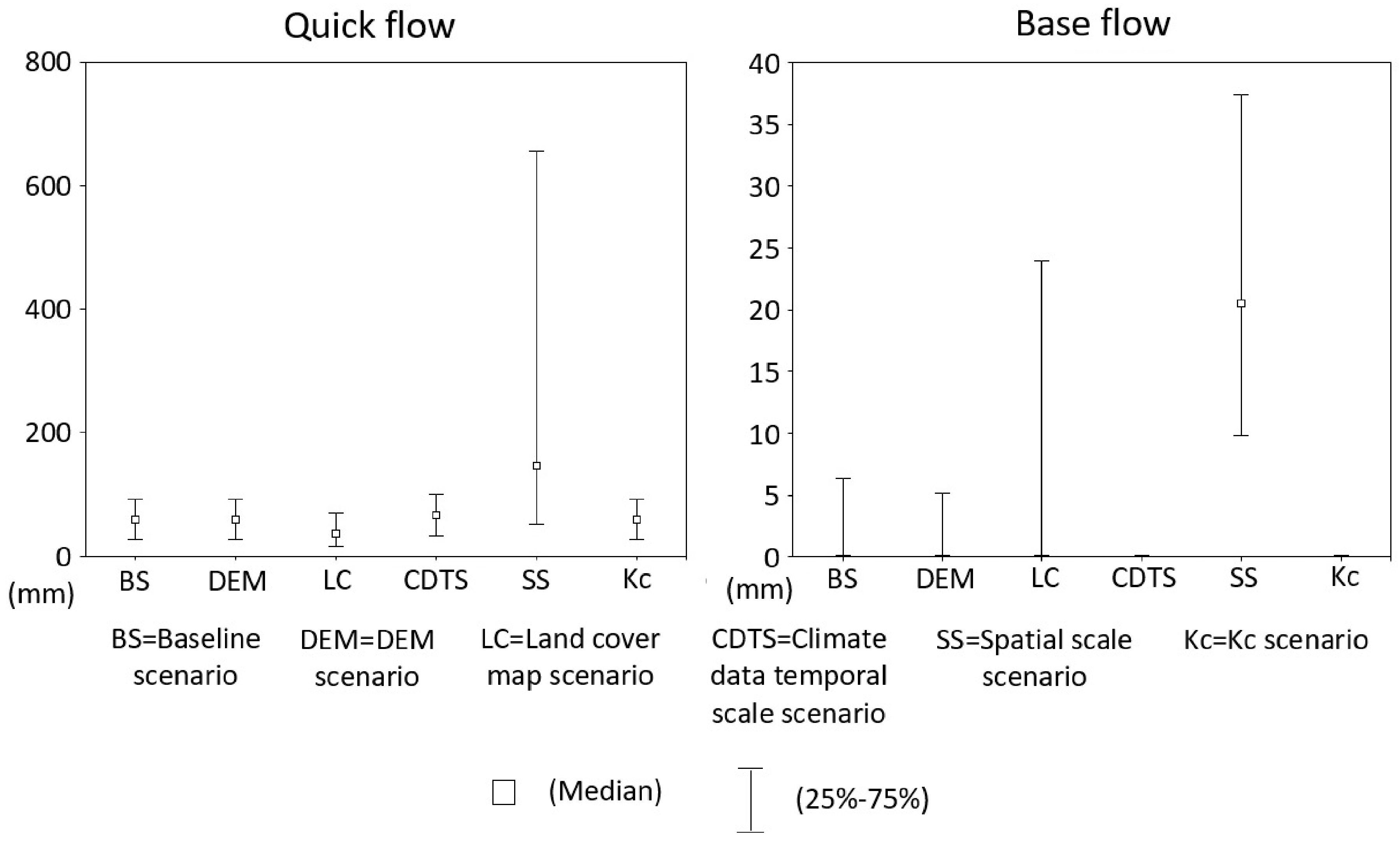
In this section, we first analysed the quick flow outputs by comparing the Baseline scenario to the results for the uncertainty scenarios. Under the Baseline scenario, the quick flow maps (Figure 2) showed that the highest pixel value was 1662 mm, while the median value was only 59 mm (Figure 3). The values between the first quartile and the third quartile ranged from 28 mm to 92 mm. The highest value was located on the stream pixels in the northeast edge of the region. Besides the stream network, there were large apparent differences in spatial distribution across the region. Large areas with high quick flow values were found in the north-eastern and eastern edge and scattered across the cropping land and the mining footprint. Besides these high value areas, other regions had comparatively lower values.
A qualitative comparison between the Baseline and uncertainty scenarios (Figure 2 and Figure 3) showed that the spatial distribution of quick flow for all the uncertainty scenarios apart from spatial scale were almost the same as the Baseline. High values were mainly distributed along the stream network and in the north-eastern part, the values of other areas were comparatively low. The stream quick flow of Spatial scale scenario was uniquely different to the Baseline and other uncertainty scenarios in terms of spatial distribution (Figure 2) and overall values (Figure 3).
The relative spatial differences of pixel values between uncertainty scenarios and Baseline scenarios for quick flow are shown in Figure 4. The DEM scenario showed the largest differences; especially for the stream pixels, with the maximum positive value of 1472 mm and the minimum negative value of −1473 mm, however these differences were confined to a few pixels. The Land cover map scenario showed much more heterogeneous differences i.e. higher in cropping areas while lower in the mining footprint area. The difference associated with the Climate data temporal scale scenario were less than the above two scenarios with values ranging from −127 mm to 123 mm, which mainly occurred in the eastern part of the region. For the Spatial scale scenario maps, the pixel values in most of the region were higher, among which the highest value was 1467 mm. In contrast to the other scenarios, there was no difference between the Baseline and Kc scenario for quick flow.
In terms of distribution of the pixel values for the quick flow maps, the maximum values were similar to each other and the Baseline scenario with the highest value of 1666 mm for the Climate data temporal scale scenario and the lowest value of 1649 mm for the Spatial scale scenario (Figure 2). However, the value for the 25th percentile and 75th percentile was much lower compared with the maximum value and varied between scenarios (Figure 3). The range between the 25th percentile and 75th percentile for the Spatial scale scenario was the highest at 52 mm to 656 mm respectively. While the Land cover map scenario was the lowest with values of 17 mm to 70 mm for the 25th and 75th percentile. The DEM, Climate data temporal scale and Kc scenarios had similar ranges to the baseline.
The base flow maps (Figure 2) also showed large differences in the spatial patterns between scenarios. The spatial distribution of pixel values for the DEM scenario and Spatial scale scenario overall were approximately the same as the Baseline scenario, where high values were mainly located at the eastern edge, mining footprints and central-southern area. Though at fine scales there was much greater heterogeneity in the values of the Spatial scale scenario. The Climate data temporal scale and Kc scenarios had only very few areas with comparatively high values. Besides the differences in spatial pattern, pixel value distributions also showed differences (Figure 3). A maximum value of 1103 mm for the Land cover map scenario was 162 mm higher than that of the Baseline scenario. While the maximum values of other scenarios were all much less than the 940 mm of the Baseline scenario. The value ranges between the 25th and 75th percentile were much lower than the maximum values, among which the first quartile values of all scenarios were 0; except for the Spatial scale scenario with a value of 9.77 mm. The values of Kc scenario and Climate data temporal scale scenario were so small that even the third quartile values were 0. The differences in pixel values for base flow are shown in Figure 4. The DEM scenario and Land cover map scenario had unique patterns of differences compared to the other scenarios. The Climate data temporal scale scenario and Kc scenario showed smaller values at the eastern boundary (coast), mining footprint and central southern area. The Spatial scale scenario tended to have higher pixel values across the region with the highest value of 554 mm.
3.2. Value Comparisons for Particular Land Uses
To quantify the impact of uncertainty scenarios for different land uses, the RVC index was utilized to calculate the base flow and quick flow differences between the baseline and uncertainty scenarios. The RVC index value was normalized with the values ranging between 0 and 1 and a higher value indicating a greater difference. Figure 5 showed the RVC indices of different scenarios for the four main land use types which occupied more than 99% of the total area and the mean RVC value of all land use types (including all the main and small covers). For the quick flow, the RVC values of Spatial scale scenario were the highest in all the different areas, among which the maximum value was 0.80 in forestry. The highest value of the other scenarios in forestry was only 0.03 for the Climate data temporal scale scenario, which was much lower than the value for the Spatial scale scenario. For other areas not including forestry, the RVC values of Land cover map scenario were the second highest after the Spatial scale scenario and much higher than the other scenarios. The lowest value was 0 in Kc scenario for all of the four land uses.
For the base flow for all of the four land use areas, the RVC values of Kc and Climate data temporal scale scenarios were much higher than the values of the other three scenarios, among which the highest value was 0.98 for mining footprint area under Climate data temporal scale scenario. The value distribution of the other three scenarios for the mining area ranged from 0.02 to 0.17, which were much lower than those for cropping, forestry and grazing area. The Land cover map scenario produced the lowest RVC value of 0.02 in mining areas while the lowest value for the other land uses were found in the DEM scenario. The RVC values of all land uses under Kc and Climate data temporal scale scenarios were also much higher than for the other scenarios.
3.3. Catchment-Scale Annual Total Water Yield
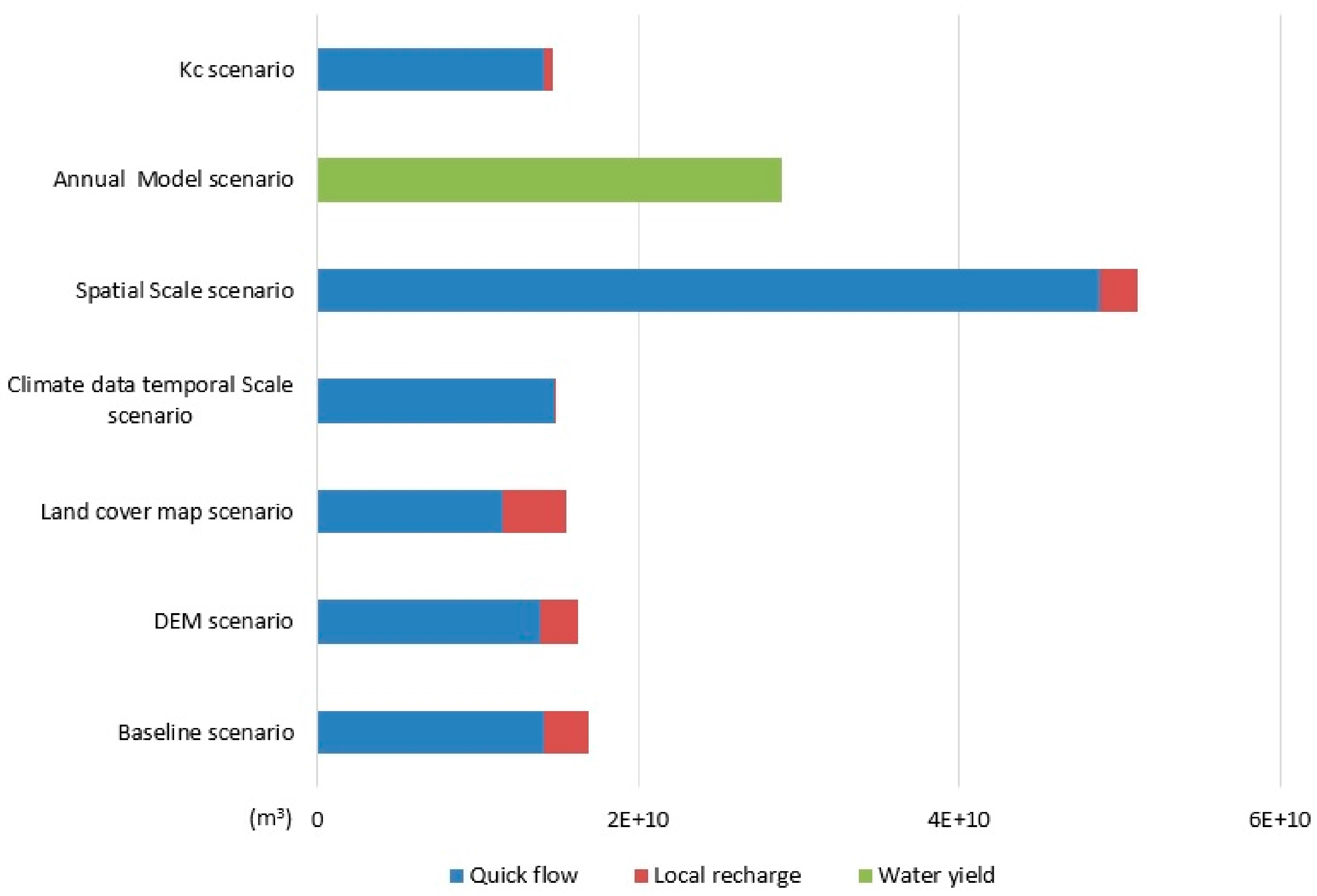
Annual total water yield represents water provisioning at the whole catchment scale. The water yield amount for the Annual model scenario was a direct output from the annual water yield model, while the value for other scenarios using the Seasonal water yield model were the sum of quick flow and local recharge. Figure 6 represents the annual total water yield volume of all seven scenarios. The total volume of water yield for the Baseline scenario was 1.69 × 10¹⁰ m3 and was less than the values 5.12 × 10¹⁰ m3 of Spatial scale scenario and 2.8951 × 10¹⁰ m3 of Annual model scenario. While the total volume from Climate data temporal scale (1.49 × 10¹⁰ m3), DEM (1.62 × 10¹⁰ m3), Land cover map (1.56 × 10¹⁰ m3), Kc (1.47 × 10¹⁰ m3) scenarios were less than the Baseline scenario with the Kc scenario producing the lowest water volume.
4. Discussion
4.1. Impact of Uncertainty on Water Provision
The Baseline scenario outputs represented the current water provision service condition of the study area. As previously observed in a previous study area [85], the average water flow volume of the Fitzroy River and Isaac river sub-catchments were much higher than other sub-catchments, which was in accordance with the general spatial patterns in our study. Similarly, erosion research in this area [86,87,88] showed water quantity spatial distributions comparable to our study with values of both the quick flow and base flow high in the eastern sections. The reason for this spatial distribution is due to higher elevation and topographical heterogeneity and high annual precipitation in these regions [74,89,90,91] which generate higher stream flow and local recharge. In the mining area which was mainly occupied by bare pits, coal stockpile and industrial plants, the poor permeability (high runoff curve number) resulted in high quick flow [63], while the low evapotranspiration affected the recharge to base flow. In addition, the comparatively high quick flow of cropping land was also a result of hydrologic conditions associated with high runoff curve numbers, which are always accompanied by large amount of soil loss [59,92].
The scenarios analysis demonstrated how uncertainties derived from the mapping and modelling methods affects ecosystem service modelling outputs and that the sensitivity of different outputs (i.e., base flow versus quick flow) varied with the uncertainty scenario. The uncertainties in quick flow associated with plant evapotranspiration (Kc scenario) were minor compared to the baseline. While changes to topography under the spatial scale and DEM scenario lead to different stream directions and water flow values. Of the uncertainty factors assessed, a coarsening of spatial scale (Spatial scale scenario) had the greatest effect on both overall values, spatial distribution of values and even the characterization of stream direction which corresponds with findings of other studies such as [15,75]. For base flow, spatial patterns and values changed with all uncertainty scenarios except for the DEM scenario. Differences due to the Climate data temporal scale, Kc and Land cover map scenarios show that uncertainty associated with precipitation, evapotranspiration, plant factors and land classification schemes affect modelling outcomes. These factors have also been recognized as key variables affecting relevant ecosystem services in other studies [24,93,94]. A critical and interesting result of this study was from the Climate data temporal scale scenario which showed that ignoring distinctive wet and dry seasons by using an annual model are likely to produce model outputs that are less likely to reflect true values.
Another interesting observation from the analysis were that literature-based parameterization resulted in very different modelling outputs than direct measurements. For example, for the Kc scenario, the literature-based Kc of forest was between 0.5 and 1.2 [52] while the remote sensing measured Kc values ranged from 0.56 to 0.80. Reason for this difference is that the vegetation characteristics of the forests in the study area are characterized by sparse vegetation in contrast to the less open forests from the locations in the literature [95,96]. In addition, the literature-based Kc value were from more developed locations with less vegetation and thus had lower Kc values of 0.2 for industrial land and 0.3 for urban residential area [26,52].
Of all the scenarios, the Spatial scale scenario had the greatest overall impact. Spatial scale affects climate, land cover, plant parameters and the DEM. The large apparent impact of spatial scale scenario for both quick flow and base flow demonstrates, as shown in many studies, that scale is a critical driver of uncertainty in spatially explicit modelling [15,39,97]. As well as impacts on spatial patterns of quick and base flow, this study also developed and utilized the RVC index to quantify water provision changes under the uncertainty scenarios for specific land uses. The RVC analysis of quick flow showed that the Land cover map and Spatial scale scenarios had higher average RVC values than other scenarios, which are likely to be caused by the spatial variability in the runoff curve numbers and DEM [98,99]. In contrast for the base flow, the average RVC values for Kc and Climate data temporal scale scenario had much higher values than for other scenarios. Similar trends were found with the RVC assessment in the qualitative analysis of spatial patterns with distinct RVC values in different areas.
The final assessment based on the annual total water yield of a catchment represents the water provision ability and hydrological conditions of the catchment [100,101,102]. Previous studies in the region on the annual water yield volume were mainly from gauged stream flow during wet season [85,87]. These studies provide water yield volumes based on distinctive weather conditions for specific years as opposed to average climate condition used in our modelling. For example, Jones et al. gauged total stream flow volume were 2.16 × 10¹⁰ m3 in 2012/13 and 4.96 × 10¹⁰ m3 in 2013/14 [85], which are similar to the water yield value for the Baseline scenario of 1.69 × 10¹⁰ m3. However, under different uncertainty scenarios such as spatial scale the values were much higher. The differences between the uncertainty scenarios and gauged total stream flow volume were in the same order of magnitude suggesting that even the outputs from the uncertainty scenarios are likely to provide some useful information.
4.2. ES Mapping Uncertainty in the Context of the Fitzroy Basin and Mining
This study used the water provision mapping in the Fitzroy Basin mining region as a case study to quantify uncertainties in ES mapping. The differences in outputs associated with each uncertainty scenario reflect the result of using models, parameterization and data that could reasonably be used for mapping ES. Our study found relatively large differences in model outputs due to uncertainty, demonstrating the need to identify and categorize uncertainty sources when conducting analyses [33,35]. The consideration, identification and categorization of uncertainties are likely to be different and specific to an application due to differences in data sources, catchment characteristics etc. [103,104,105]. The choice of uncertainty methods assessment selection are an important consideration as uncertainty assessment can be complex and time-consuming [33]. This study applied scenario analysis in an uncertainty assessment, which is common and considered to be an effective approach [35,38,41]. However, as spatial data and modelling for ES mapping is complex with almost an infinite source of uncertainty, it is difficult to characterize all sources of uncertainties in the spatial attributes of ES. Spatial data are more complex than parametric values and different observation scales may lead to different outcomes and the accuracy of each pixel may be distinctive [33].
The application of uncertainty analysis such as for assessing mining impacts is difficult from the perspective of decision makers. Some researchers have argued that most uncertainty analysis do not assist decision-makers due to the non-practical outputs [33,106,107]. Our study offers spatially explicit maps and statistical diagrams, which provide decision-makers and stakeholders with explicit information on how these uncertainties are distributed.
The information provided by ES studies such as ours need to be interpreted with caution due to the inherent uncertainty associated with modelling methods. Our study provides information on water provision conditions such as hotspot areas and annual volumes that could potentially improve hydrological ecosystem management for management of Great Barrier Reef catchments and for assessing impacts associated with economically valuable minerals production [59,108,109] as water provision could affect either the reef environment or the large water demands from the mining industry in the region [110,111]. There needs to be and there is a large focus on planning for water resources and regional ecological sustainable development in the Fitzroy Basin [50,86,112]. However, management also need to consider uncertainty and the limitations associated with modelling outputs used to inform decision making.
5. Conclusions
This study mapped water provision ES service, quantifying uncertainties within the ES mapping process in one of the largest mining resources region in Australia. This study demonstrated the diversity of uncertainties associated with ES mapping and the many ways in which uncertainty can affect mapping outputs from spatial patterns to total water provision. The results showed that varying mapping scales had the highest impact on uncertainty. However, most forms of uncertainty led to changes in ES mapping outputs i.e. data source, parameters and mapping methods. This study provides a useful demonstration of the impact of uncertainty that is likely to be present in many ES mapping applications, prompting greater need for further research on uncertainty in ES mapping.
Acknowledgments
This research was supported by the UQ-CSC scholarship provided by The University of Queensland and China Scholarship Council. The authors would like to thank Kristen Williams and Dominic Hogan for their assistance on the CSIRO spatial dataset provision and application; and Chris Ryan for his support on the software license of CatchmentSIM.
Author Contributions
Zhenyu Wang and Alex Mark Lechner designed the project; Zhenyu Wang performed the analysis and led the writing of the paper; Alex Mark Lechner and Thomas Baumgartl provided advice on the topic and analysis and contributed to writing of the paper.
Conflicts of Interest
The authors declare no conflict of interest.
Appendix A

Table A1.
Monthly Kc values for each land classification under Baseline scenario.
| Land Classification | Kc_1 | Kc_2 | Kc_3 | Kc_4 | Kc_5 | Kc_6 | Kc_7 | Kc_8 | Kc_9 | Kc_10 | Kc_11 | Kc_12 |
|---|---|---|---|---|---|---|---|---|---|---|---|---|
| Cropping | 0.37 | 0.50 | 0.54 | 0.40 | 0.33 | 0.27 | 0.27 | 0.29 | 0.27 | 0.27 | 0.22 | 0.29 |
| Horticulture | 0.74 | 0.82 | 0.80 | 0.67 | 0.59 | 0.52 | 0.47 | 0.42 | 0.46 | 0.57 | 0.60 | 0.67 |
| Forestry | 0.60 | 0.68 | 0.76 | 0.79 | 0.80 | 0.78 | 0.73 | 0.66 | 0.62 | 0.61 | 0.56 | 0.58 |
| Rural residential | 0.62 | 0.73 | 0.78 | 0.62 | 0.54 | 0.46 | 0.40 | 0.35 | 0.36 | 0.44 | 0.42 | 0.50 |
| Urban residential | 0.47 | 0.56 | 0.60 | 0.51 | 0.46 | 0.39 | 0.34 | 0.29 | 0.30 | 0.36 | 0.31 | 0.37 |
| Utilities and Services | 0.48 | 0.58 | 0.62 | 0.51 | 0.45 | 0.37 | 0.32 | 0.29 | 0.30 | 0.36 | 0.30 | 0.38 |
| Transport | 0.48 | 0.61 | 0.62 | 0.46 | 0.38 | 0.31 | 0.24 | 0.22 | 0.25 | 0.32 | 0.26 | 0.34 |
| Grazing | 0.53 | 0.65 | 0.68 | 0.56 | 0.49 | 0.40 | 0.33 | 0.29 | 0.31 | 0.38 | 0.34 | 0.41 |
| Industrial | 0.34 | 0.43 | 0.48 | 0.39 | 0.33 | 0.25 | 0.20 | 0.18 | 0.19 | 0.25 | 0.20 | 0.26 |
| Bare land | 0.20 | 0.25 | 0.31 | 0.26 | 0.22 | 0.16 | 0.10 | 0.08 | 0.10 | 0.13 | 0.10 | 0.14 |
| Water | 0.32 | 0.39 | 0.42 | 0.34 | 0.29 | 0.23 | 0.20 | 0.18 | 0.19 | 0.23 | 0.19 | 0.24 |
Table A2.
Monthly Kc values for each land classification under Land cover map scenario.
| Land Classification | Kc_1 | Kc_2 | Kc_3 | Kc_4 | Kc_5 | Kc_6 | Kc_7 | Kc_8 | Kc_9 | Kc_10 | Kc_11 | Kc_12 |
|---|---|---|---|---|---|---|---|---|---|---|---|---|
| Extraction Sites | 0.15 | 0.19 | 0.24 | 0.20 | 0.17 | 0.12 | 0.08 | 0.06 | 0.08 | 0.10 | 0.08 | 0.11 |
| Inland Waterbodies | 0.21 | 0.25 | 0.28 | 0.22 | 0.19 | 0.16 | 0.15 | 0.14 | 0.13 | 0.14 | 0.12 | 0.15 |
| Irrigated Cropping | 0.75 | 0.84 | 0.87 | 0.79 | 0.75 | 0.71 | 0.65 | 0.57 | 0.58 | 0.66 | 0.65 | 0.73 |
| Rainfed Cropping | 0.32 | 0.46 | 0.51 | 0.38 | 0.32 | 0.26 | 0.26 | 0.27 | 0.25 | 0.22 | 0.18 | 0.25 |
| Rainfed Pasture | 0.56 | 0.71 | 0.69 | 0.50 | 0.39 | 0.29 | 0.22 | 0.21 | 0.25 | 0.34 | 0.30 | 0.37 |
| Tussock Grasses Open | 0.49 | 0.63 | 0.62 | 0.44 | 0.34 | 0.24 | 0.18 | 0.17 | 0.21 | 0.28 | 0.26 | 0.32 |
| Hummock Grasses Sparse | 0.31 | 0.39 | 0.43 | 0.33 | 0.29 | 0.20 | 0.14 | 0.13 | 0.16 | 0.21 | 0.17 | 0.24 |
| Tussock Grasses Sparse | 0.29 | 0.44 | 0.52 | 0.38 | 0.31 | 0.20 | 0.17 | 0.15 | 0.16 | 0.19 | 0.16 | 0.22 |
| Shrubs Closed | 0.35 | 0.42 | 0.46 | 0.42 | 0.40 | 0.31 | 0.24 | 0.20 | 0.23 | 0.28 | 0.23 | 0.32 |
| Shrubs Sparse | 0.48 | 0.61 | 0.59 | 0.43 | 0.33 | 0.25 | 0.19 | 0.19 | 0.23 | 0.31 | 0.27 | 0.34 |
| Chenopod Shrubs Sparse | 0.25 | 0.36 | 0.44 | 0.35 | 0.29 | 0.19 | 0.14 | 0.12 | 0.15 | 0.18 | 0.15 | 0.19 |
| Trees Closed | 0.82 | 0.89 | 0.96 | 0.97 | 0.96 | 0.94 | 0.92 | 0.89 | 0.86 | 0.86 | 0.78 | 0.81 |
| Trees Open | 0.61 | 0.70 | 0.77 | 0.78 | 0.77 | 0.73 | 0.67 | 0.60 | 0.57 | 0.58 | 0.52 | 0.56 |
| Trees Scattered | 0.42 | 0.52 | 0.53 | 0.42 | 0.36 | 0.27 | 0.20 | 0.17 | 0.22 | 0.28 | 0.25 | 0.32 |
| Trees Sparse | 0.51 | 0.63 | 0.67 | 0.56 | 0.49 | 0.41 | 0.33 | 0.30 | 0.32 | 0.38 | 0.33 | 0.40 |
Table A3.
Biophysical parameters for Annual model scenario.
| Land Classification | Kc | Root Depth (mm) | LULC_veg |
|---|---|---|---|
| Cropping | 0.34 | 1500 | 1 |
| Horticulture | 0.64 | 5000 | 1 |
| Forestry | 0.66 | 5000 | 1 |
| Rural residential | 0.53 | −1 | 0 |
| Urban residential | 0.42 | −1 | 0 |
| Utilities and Services | 0.42 | −1 | 0 |
| Transport | 0.39 | −1 | 0 |
| Grazing | 0.46 | 1000 | 1 |
| Industrial | 0.30 | −1 | 0 |
| Bare land | 0.18 | −1 | 0 |
| Water | 0.28 | −1 | 0 |
Table A4.
Monthly Kc values for each land classification under Kc scenario.
| Land Classification | Kc_1 | Kc_2 | Kc_3 | Kc_4 | Kc_5 | Kc_6 | Kc_7 | Kc_8 | Kc_9 | Kc_10 | Kc_11 | Kc_12 |
|---|---|---|---|---|---|---|---|---|---|---|---|---|
| Cropping | 1 | 1 | 0.85 | 0.65 | 0.5 | 0.3 | 0.35 | 0.35 | 0.35 | 0.35 | 0.5 | 0.7 |
| Horticulture | 1 | 1 | 0.75 | 0.75 | 0.75 | 0.65 | 0.65 | 0.65 | 0.65 | 0.7 | 0.75 | 1 |
| Forestry | 1.2 | 1.2 | 1.2 | 1 | 1 | 0.5 | 0.5 | 0.5 | 0.5 | 0.5 | 1 | 1 |
| Rural residential | 0.6 | 0.6 | 0.6 | 0.4 | 0.4 | 0.4 | 0.4 | 0.4 | 0.4 | 0.4 | 0.6 | 0.6 |
| Urban residential | 0.3 | 0.3 | 0.3 | 0.3 | 0.3 | 0.3 | 0.3 | 0.3 | 0.3 | 0.3 | 0.3 | 0.3 |
| Utilities and Services | 0.1 | 0.1 | 0.1 | 0.1 | 0.1 | 0.1 | 0.1 | 0.1 | 0.1 | 0.1 | 0.1 | 0.1 |
| Transport | 0.1 | 0.1 | 0.1 | 0.1 | 0.1 | 0.1 | 0.1 | 0.1 | 0.1 | 0.1 | 0.1 | 0.1 |
| Grazing | 0.85 | 0.8 | 0.75 | 0.75 | 0.7 | 0.5 | 0.3 | 0.3 | 0.3 | 0.5 | 0.7 | 0.8 |
| Industrial | 0.2 | 0.2 | 0.2 | 0.2 | 0.2 | 0.2 | 0.2 | 0.2 | 0.2 | 0.2 | 0.2 | 0.2 |
| Bare land | 0.5 | 0.5 | 0.5 | 0.5 | 0.5 | 0.5 | 0.5 | 0.5 | 0.5 | 0.5 | 0.5 | 0.5 |
| Water | 1 | 1 | 1 | 1 | 0.6 | 0.6 | 0.6 | 0.6 | 0.6 | 0.6 | 1 | 1 |
References
- Costanza, R.; d’Arge, R.; de Groot, R.; Farber, S.; Grasso, M.; Hannon, B.; Limburg, K.; Naeem, S.; O’Neill, R.V.; Paruelo, J.; et al. The value of the world’s ecosystem services and natural capital. Nature 1997, 387, 253–260. [Google Scholar] [CrossRef]
- De Groot, R.S.; Wilson, M.A.; Boumans, R.M.J. A typology for the classification, description and valuation of ecosystem functions, goods and services. Ecol. Econ. 2002, 41, 393–408. [Google Scholar] [CrossRef]
- Millennium Ecosystem Assessment (MEA). Ecosystems and Human Well-Being: Synthesis; Island Press: Washington, DC, USA, 2005. [Google Scholar]
- The Economics of Ecosystems and Biodiversity (TEEB). Mainstreaming the Economics of Nature: A Synthesis of the Approach, Conclusions and Recommendations of TEEB; TEEB: Geneva, Switzerland, 2010.
- Daily, G.C.; Matson, P.A. Ecosystem Services: From Theory to Implementation. Proc. Natl. Acad. Sci. USA 2008, 105, 9455–9456. [Google Scholar] [CrossRef] [PubMed]
- Maes, J.; Hauck, J.; Paracchini, M.L.; Ratamäki, O.; Hutchins, M.; Termansen, M.; Furman, E.; Pérez-Soba, M.; Braat, L.; Bidoglio, G. Mainstreaming ecosystem services into EU policy. Curr. Opin. Environ. Sustain. 2013, 5, 128–134. [Google Scholar] [CrossRef]
- Grêt-Regamey, A.; Celio, E.; Klein, T.M.; Wissen Hayek, U. Understanding ecosystem services trade-offs with interactive procedural modelling for sustainable urban planning. Landsc. Urban Plan. 2013, 109, 107–116. [Google Scholar] [CrossRef]
- Albert, C.; Galler, C.; Hermes, J.; Neuendorf, F.; Von Haaren, C.; Lovett, A. Applying ecosystem services indicators in landscape planning and management: The ES-in-Planning framework. Ecol. Indic. 2016, 61, 100–113. [Google Scholar] [CrossRef]
- Mavsar, R.; Kova, M. Forest Policy and Economics Trade-offs between FI RE prevention and provision of ecosystem services in Slovenia. For. Policy Econ. 2013, 29, 62–69. [Google Scholar] [CrossRef]
- Matthews, S.N.; Iverson, L.R.; Peters, M.P.; Prasad, A.M.; Subburayalu, S. Assessing and comparing risk to climate changes among forested locations: Implications for ecosystem services. Landsc. Ecol. 2013, 29, 213–228. [Google Scholar] [CrossRef]
- Martinez-Harms, M.J.; Bryan, B.A.; Balvanera, P.; Law, E.A.; Rhodes, J.R.; Possingham, H.P.; Wilson, K.A. Making decisions for managing ecosystem services. Biol. Conserv. 2015, 184, 229–238. [Google Scholar] [CrossRef]
- Daily, G.C.; Polasky, S.; Goldstein, J.; Kareiva, P.M.; Mooney, H.A.; Pejchar, L.; Ricketts, T.H.; Salzman, J.; Shallenberger, R. Ecosystem services in decision making: Time to deliver. Front. Ecol. Environ. 2009, 7, 21–28. [Google Scholar] [CrossRef]
- Goldstein, J.H.; Caldarone, G.; Duarte, T.K.; Ennaanay, D.; Hannahs, N.; Mendoza, G.; Polasky, S.; Wolny, S.; Daily, G.C. Integrating ecosystem-service tradeoffs into land-use decisions. Proc. Natl. Acad. Sci. USA 2012, 109, 7565–7570. [Google Scholar] [CrossRef] [PubMed]
- Peh, K.S.H.; Thapa, I.; Basnyat, M.; Balmford, A.; Bhattarai, G.P.; Bradbury, R.B.; Brown, C.; Butchart, S.H.M.; Dhakal, M.; Gurung, H.; et al. Synergies between biodiversity conservation and ecosystem service provision: Lessons on integrated ecosystem service valuation from a Himalayan protected area, Nepal. Ecosyst. Serv. 2015, 22, 359–369. [Google Scholar] [CrossRef]
- Grêt-Regamey, A.; Weibel, B.; Bagstad, K.J.; Ferrari, M.; Geneletti, D.; Klug, H.; Schirpke, U.; Tappeiner, U. On the effects of scale for ecosystem services mapping. PLoS ONE 2014, 9, e112601. [Google Scholar] [CrossRef] [PubMed]
- Brunner, S.H.; Huber, R.; Grêt-Regamey, A. Mapping uncertainties in the future provision of ecosystem services in a mountain region in Switzerland. Reg. Environ. Chang. 2017, 17, 2309–2321. [Google Scholar] [CrossRef]
- Crossman, N.D.; Burkhard, B.; Nedkov, S.; Willemen, L.; Petz, K.; Palomo, I.; Drakou, E.G.; Martín-Lopez, B.; McPhearson, T.; Boyanova, K.; et al. A blueprint for mapping and modelling ecosystem services. Ecosyst. Serv. 2013, 4, 4–14. [Google Scholar] [CrossRef]
- Martínez-Harms, M.J.; Balvanera, P. Methods for mapping ecosystem service supply: A review. Int. J. Biodivers. Sci. Ecosyst. Serv. Manag. 2012, 8, 17–25. [Google Scholar] [CrossRef]
- Maes, J.; Egoh, B.; Willemen, L.; Liquete, C.; Vihervaara, P.; Schägner, J.P.; Grizzetti, B.; Drakou, E.G.; La Notte, A.; Zulian, G.; et al. Mapping ecosystem services for policy support and decision making in the European Union. Ecosyst. Serv. 2012, 1, 31–39. [Google Scholar] [CrossRef]
- Burkhard, B.; Kroll, F.; Nedkov, S.; Müller, F. Mapping ecosystem service supply, demand and budgets. Ecol. Indic. 2012, 21, 17–29. [Google Scholar] [CrossRef]
- Egoh, B.; Reyers, B.; Rouget, M.; Richardson, D.M.; Le Maitre, D.C.; van Jaarsveld, A.S. Mapping ecosystem services for planning and management. Agric. Ecosyst. Environ. 2008, 127, 135–140. [Google Scholar] [CrossRef]
- Egoh, B.; Drakou, E.G.; Dunbar, M.B.; Maes, J. Indicators for Mapping Ecosystem Services: A Review; Publications Office of the European Union: Luxembourg, 2012. [Google Scholar]
- Ayanu, Y.Z.; Conrad, C.; Nauss, T.; Wegmann, M.; Koellner, T. Quantifying and mapping ecosystem services supplies and demands: A review of remote sensing applications. Environ. Sci. Technol. 2012, 46, 8529–8541. [Google Scholar] [CrossRef] [PubMed]
- Haines-Young, R.; Potschin, M.; Kienast, F. Indicators of ecosystem service potential at European scales: Mapping marginal changes and trade-offs. Ecol. Indic. 2012, 21, 39–53. [Google Scholar] [CrossRef]
- Plieninger, T.; Dijks, S.; Oteros-Rozas, E.; Bieling, C. Assessing, mapping and quantifying cultural ecosystem services at community level. Land Use Policy 2013, 33, 118–129. [Google Scholar] [CrossRef]
- Sharp, E.R.; Chaplin-kramer, R.; Wood, S.; Guerry, A.; Tallis, H.; Ricketts, T.; Authors, C.; Nelson, E.; Ennaanay, D.; Wolny, S.; et al. InVEST +VERSION+ User’s Guide; The Natural Capital Project; Stanford University: Stanford, CA, USA; University of Minnesota: Minneapolis, MN, USA; The Nature Conservancy: Arlington, VA, USA; WorldWildlife Fund: Gland, Switzerland, 2016. [Google Scholar]
- Villa, F.; Bagstad, K.J.; Voigt, B.; Johnson, G.W.; Portela, R.; Honzák, M.; Batker, D. A methodology for adaptable and robust ecosystem services assessment. PLoS ONE 2014, 9, e91001. [Google Scholar] [CrossRef] [PubMed]
- Burkhard, B.; Crossman, N.; Nedkov, S.; Petz, K.; Alkemade, R. Mapping and modelling ecosystem services for science, policy and practice. Ecosyst. Serv. 2013, 4, 1–3. [Google Scholar] [CrossRef]
- Yee, S.H.; Dittmar, J.A.; Oliver, L.M. Comparison of methods for quantifying reef ecosystem services: A case study mapping services for St. Croix; USVI. Ecosyst. Serv. 2014, 8, 1–15. [Google Scholar] [CrossRef]
- Vorstius, A.C.; Spray, C.J. A comparison of ecosystem services mapping tools for their potential to support planning and decision-making on a local scale. Ecosyst. Serv. 2015, 15, 75–83. [Google Scholar] [CrossRef]
- Tallis, H.; Polasky, S. Mapping and valuing ecosystem services as an approach for conservation and natural-resource management. Ann. N. Y. Acad. Sci. 2009, 1162, 265–283. [Google Scholar] [CrossRef] [PubMed]
- Serna-Chavez, H.M.; Schulp, C.J.E.; Van Bodegom, P.M.; Bouten, W.; Verburg, P.H.; Davidson, M.D. A quantitative framework for assessing spatial flows of ecosystem services. Ecol. Indic. 2014, 39, 24–33. [Google Scholar] [CrossRef]
- Hamel, P.; Bryant, B.P. Uncertainty assessment in ecosystem services analyses: Common challenges and practical responses. Ecosyst. Serv. J. 2017, 24, 1–15. [Google Scholar] [CrossRef]
- Grêt-Regamey, A.; Brunner, S.H.; Altwegg, J.; Bebi, P. Facing uncertainty in ecosystem services-based resource management. J. Environ. Manag. 2012, 127, S145–S154. [Google Scholar] [CrossRef] [PubMed]
- Hou, Y.; Burkhard, B.; Müller, F. Uncertainties in landscape analysis and ecosystem service assessment. J. Environ. Manag. 2013, 127, S117–S131. [Google Scholar] [CrossRef] [PubMed]
- Schulp, C.J.E.; Burkhard, B.; Maes, J.; Van Vliet, J.; Verburg, P.H. Uncertainties in Ecosystem Service Maps: A Comparison on the European Scale. PLoS ONE 2014, 9, e109643. [Google Scholar] [CrossRef] [PubMed] [Green Version]
- Blasone, R.-S.; Madsen, H.; Rosbjerg, D. Uncertainty assessment of integrated distributed hydrological models using GLUE with Markov chain Monte Carlo sampling. J. Hydrol. 2008, 353, 18–32. [Google Scholar] [CrossRef] [Green Version]
- Benke, K.K.; Pettit, C.J.; Lowell, K.E. Visualisation of spatial uncertainty in hydrological modelling. J. Spat. Sci. 2011, 56, 73–88. [Google Scholar] [CrossRef]
- Lechner, A.M.; Langford, W.T.; Bekessy, S.A.; Jones, S.D. Are landscape ecologists addressing uncertainty in their remote sensing data? Landsc. Ecol. 2012, 27, 1249–1261. [Google Scholar] [CrossRef]
- Surfleet, C.G.; Tullos, D. Uncertainty in hydrologic modelling for estimating hydrologic response due to climate change (Santiam River, Oregon). Hydrol. Process. 2013, 27, 3560–3576. [Google Scholar] [CrossRef]
- Woodward, S.J.R.; Wöhling, T.; Stenger, R. Uncertainty in the modelling of spatial and temporal patterns of shallow groundwater flow paths: The role of geological and hydrological site information. J. Hydrol. 2016, 534, 680–694. [Google Scholar] [CrossRef]
- Fagerholm, N.; Käyhkö, N.; Ndumbaro, F.; Khamis, M. Community stakeholders’ knowledge in landscape assessments—Mapping indicators for landscape services. Ecol. Indic. 2012, 18, 421–433. [Google Scholar] [CrossRef]
- Gos, P.; Lavorel, S. Stakeholders’ expectations on ecosystem services affect the assessment of ecosystem services hotspots and their congruence with biodiversity. Int. J. Biodivers. Sci. Ecosyst. Serv. Manag. 2012, 8, 93–106. [Google Scholar] [CrossRef]
- Butler, J.R.A.; Wong, G.Y.; Metcalfe, D.J.; Honzák, M.; Pert, P.L.; Rao, N.; van Grieken, M.E.; Lawson, T.; Bruce, C.; Kroon, F.J.; et al. An analysis of trade-offs between multiple ecosystem services and stakeholders linked to land use and water quality management in the Great Barrier Reef, Australia. Agric. Ecosyst. Environ. 2013, 180, 176–191. [Google Scholar] [CrossRef]
- Grêt-Regamey, A.; Brunner, S.H.; Altwegg, J.; Christen, M.; Bebi, P. Integrating Expert Knowledge into Mapping Ecosystem Services Trade-offs for Sustainable Forest Management. Ecol. Soc. 2013, 18, 378–380. [Google Scholar] [CrossRef]
- Kopperoinen, L.; Itkonen, P.; Niemelä, J. Using expert knowledge in combining green infrastructure and ecosystem services in land use planning: An insight into a new place-based methodology. Landsc. Ecol. 2014, 8, 1361–1375. [Google Scholar] [CrossRef]
- Carroll, C.; Dougall, C.; Silburn, M.; Waters, D.; Packett, B.; Joo, M. Sediment erosion research in the Fitzroy Basin central Queensland: An overview. In Proceedings of the 19th World Congress of Soil Science, Brisbane, Australia, 1–6 August 2010; pp. 167–170. [Google Scholar]
- Bohnet, I.; Bohensky, E.; Gambley, C.; Waterhouse, J. Future Scenarios for the Great Barrier Reef Catchment; Water for a Healthy Country National Research Flagship (CSIRO): Canberra, Australia, 2008. [Google Scholar]
- Great Barrier Reef Marine Park Authority. Fitzroy Basin Assessment—Fitzroy Basin Association Natural Resource Management Region; GBRMPA: Townsville, Australia, 2013. [Google Scholar]
- Christensen, S.; Claire, R. Central Queensland Strategy for Sustainability 2004 and beyond; Fitzroy Basin Association: Rockhampton, Australia, 2004. [Google Scholar]
- Amit, H.; Lyakhovsky, V.; Katz, A.; Starinsky, A.; Burg, A. Interpretation of Spring Recession Curves. Ground Water 2002, 40, 543–551. [Google Scholar] [CrossRef] [PubMed]
- Allen, R.G.; Pereira, L.S.; Raes, D.; Smith, M.; Ab, W. Crop Evapotranspiration—Guidelines for Computing Crop Water Requirements—FAO Irrigation and Drainage Paper 56; Food and Agriculture Organization of the United Nations (FAO): Roma, Italy, 1998; Volume 300, pp. 1–15. [Google Scholar]
- United States Department of Agriculture (NRCS-USDA). National Engineering Handbook; United States Department of Agriculture: Washington, DC, USA, 2007.
- Geoscience Australia (GA). 3 Second SRTM Digital Elevation Model (DEM) v01; Bioregional Assessment Source Dataset: Canberra, Australia, 2010.
- Tickle, P.; Wilson, N.; Inkeep, C.; Gallant, J.; Dowling, T.; Read, A. Digital Elevation Models User Guide; GA (Geosciences Australia): Canberra, Australia, 2010. [Google Scholar]
- Williams, K. Soil aveRage Saturated Hydraulic Conductivity (A and B Horizon) in Units of mm/h; CSIRO Ecosystem Sciences: Canberra, Australia, 2011. [Google Scholar]
- Queensland Land Use Mapping Program (QLUMP). Land Use Mapping—1999 to 2009—Fitzroy NRM; Department of Science, Information Technology and Innovation: Brisbane, Australia, 2011.
- Lechner, A.M.; Kassulke, O.; Unger, C. Spatial assessment of open cut coal mining progressive rehabilitation to support the monitoring of rehabilitation liabilities. Resour. Policy 2016, 50, 234–243. [Google Scholar] [CrossRef]
- Wang, Z.; Lechner, A.M.; Baumgartl, T. Mapping cumulative impacts of mining on sediment retention ecosystem service in an Australian mining region. Int. J. Sustain. Dev. World Ecol. 2018, 25, 69–80. [Google Scholar] [CrossRef]
- Environmental Systems Research Institute (ESRI). ArcGIS Desktop: Release 10.2; Environmental Systems Research Institute: Redlands, CA, USA, 2012. [Google Scholar]
- Fan, F.; Deng, Y.; Hu, X.; Weng, Q. Estimating composite curve number using an improved SCS-CN method with remotely sensed variables in guangzhou, China. Remote Sens. 2013, 5, 1425–1438. [Google Scholar] [CrossRef] [Green Version]
- Catchment Simulation Solutions (CSS). CatchmentSIM; Catchment Simulation Solutions: Sydney, Austarlia, 2016. [Google Scholar]
- United States Department of Agriculture (USDA). Hydrology Training Series: Module 104 Runoff Curve Numver Computations Study Guide; United States Department of Agriculture: Washington, DC, USA, 1989.
- Labadz, M. A Catchment Modelling Approach Integrating Surface and Groundwater Processes, Land Use and Distribution of Nutrients: Elimbah Creek, Southeast Queensland. Ph.D. Thesis, Queensland University of Technology, Brisbane, Australia, 2012. [Google Scholar]
- Bureau of Meteorology (BOM). Climate Data Online: Weather Station Records; Australia Bureau of Meteorology: Melbourne, Australia, 2016.
- Akram, F.; Rasul, M.G.; Khan, M.M.K.; Amir, M.S.I.I. Automatic Delineation of Drainage Networks and Catchments using DEM data and GIS Capabilities: A case study. In Proceedings of the 18th Australasian Fluid Mechanics Conference, Launceston, Australia, 3–7 December 2012. [Google Scholar]
- Department of Natural Resources and Mines (DNRM). Drainage 25 k—Queensland; DNRM: Brisbane, Australia, 2007.
- Carlson, T.N.; Riziley, D.A.; Ji, J. On the Relation between NDVI, Fractional Vegetation Cover and Leaf Area Index. Remote Sens. Environ. 1997, 62, 241–252. [Google Scholar] [CrossRef]
- Lu, H.; Raupach, M.R.; Mcvicar, T.R.; Barrett, D.J. Decomposition of vegetation cover into woody and herbaceous components using AVHRR NDVI time series. Remote Sens. Environ. 2003, 86, 1–18. [Google Scholar] [CrossRef]
- Choudhury, B. Estimating Evaporation and Carbon Assimilation Using Infrared Temperature Data Vistas in Modeling. In Theory and Applications of Optical Remote Sensing; Asrar, G., Ed.; John Wiley and Sons: New York, NY, USA, 1989; pp. 628–690. [Google Scholar]
- Asrar, G.; Fuchs, M.; Kanemasu, E.; Hatfield, J. Estimating absorbed photosynthetic radiation and leaf-area index from spectral reflectance in wheat. Agron. J. 1984, 76, 300–306. [Google Scholar] [CrossRef]
- Donohue, R.; McVicar, T.; Roderick, M. Australian Monthly fPAR Derived from Advanced Very High Resolution Radiometer Reflectances—Version 5. v1. Commonwealth Scientific and Industrial Research Organisation (CSIRO): Canberra, Australia, 2013. [Google Scholar]
- Department of Natural Resources and Mines (DNRM). Digital Elevation Model—25 m—Fitzroy River Catchment—Data Package; DNRM: Brisbane, Australia, 2005.
- Vigiak, O.; Borselli, L.; Newham, L.T.H.; McInnes, J.; Roberts, A.M. Comparison of conceptual landscape metrics to define hillslope-scale sediment delivery ratio. Geomorphology 2012, 138, 74–88. [Google Scholar] [CrossRef]
- Borselli, L.; Cassi, P.; Torri, D. Prolegomena to sediment and flow connectivity in the landscape: A GIS and field numerical assessment. Catena 2008, 75, 268–277. [Google Scholar] [CrossRef]
- Geosciences Australia (GA). The National Dynamic Land Cover Dataset; GA: Canberra, Australia, 2010.
- Lechner, A.M.; Rhodes, J.R. Recent Progress on Spatial and Thematic Resolution in Landscape Ecology. Curr. Landsc. Ecol. Rep. 2016, 1, 98–105. [Google Scholar] [CrossRef]
- Openshaw, S. The Modifiable Areal Unit Problem; Concepts and Techniques in Modern Geography 38; Geo Abstracts University of East Anglia: Norwich, UK, 1984. [Google Scholar]
- Fu, B.P. On the calculation of the evaporation from land surface. Sci. Atmos. Sin. 1981, 5, 23–31. (In Chinese) [Google Scholar]
- Zhang, L.; Hickel, K.; Dawes, W.R.; Chiew, F.H.S.; Western, A.W.; Briggs, P.R. A rational function approach for estimating mean annual evapotranspiration. Water Resour. Res. 2004, 40. [Google Scholar] [CrossRef]
- Yang, H.; Yang, D.; Lei, Z.; Sun, F. New analytical derivation of the mean annual water-energy balance equation. Water Resour. Res. 2008, 44. [Google Scholar] [CrossRef]
- Donohue, R.J.; Roderick, M.L.; Mcvicar, T.R. Roots, storms and soil pores: Incorporating key ecohydrological processes into Budyko’s hydrological model. J. Hydrol. 2012, 436–437, 35–50. [Google Scholar] [CrossRef]
- Schenk, H.J.; Jackson, R.B. Rooting depths, lateral root spreads and below-ground/above-ground allometries of plants in water-limited. J. Ecol. 2002, 90, 480–494. [Google Scholar] [CrossRef]
- R Core Team. R: A Language and Environment for Statistical Computing; R Foundation for Statistical Computing: Vienna, Austria, 2015; Available online: http://www.R-project.org/ (accessed on 30 March 2017).
- Flint, N.; Jones, M.; Ukkola, L.; Eberhard, R. The Partnership Program Design for the Development of Report Cards: Phase 2, Version 2; Fitzroy Partnership for River Healthy: Rockhampton, Australia, 2014. [Google Scholar]
- Johnston, N.; Peck, G.; Ford, P.; Dougall, C.; Carroll, C. Fitzroy Basin Water Quality Improvement Report; Fitzroy Basin Association: Rockhampton, Australia, 2008. [Google Scholar]
- Dougall, C.; McCloskey, G.L.; Ellis, R.; Shaw, M.; Waters, D.; Carroll, C. Modelling Reductions of Pollutant Loads due to Improved Management Practices in the Great Barrier Reef Catchments—Fitzroy NRM Region, Technical Report Volume 6; Queensland Department of Natural Resources and Mines: Rockhampton, Australia, 2014. [Google Scholar]
- Dougall, C.; Carroll, C.; Herring, M.; Trevithick, R.; Neilsen, S.; Burger, P. Enhanced Sediment and Nutrient Modelling and Target Setting in the Fitzroy BASIN; Queensland Department of Environment and Resource Management: Brisbane, Australia, 2009. [Google Scholar]
- Yang, D.; Kanae, S.; Oki, T.; Koike, T.; Musiake, K. Global potential soil erosion with reference to land use and climate changes. Hydrol. Process. 2003, 17, 2913–2928. [Google Scholar] [CrossRef]
- Apitz, S.E. Conceptualizing the role of sediment in sustaining ecosystem services: Sediment-ecosystem regional assessment (SEcoRA). Sci. Total Environ. 2012, 415, 9–30. [Google Scholar] [CrossRef] [PubMed]
- Roth, C.H.; Prosser, I.P.; Post, D.A.; Gross, J.E.; Webb, M.J. Reducing Sediment Export from the Burdekin Catchment; CSIRO Land and Water & CSIRO Sustainable Ecosystems: Canberra, Australia, 2003. [Google Scholar]
- Brodie, J.; McKergow, L.; Prosser, I.; Furnas, M.; Hughes, A.O.; Hunter, H. Sources of Sediment and Nutrient Exports to the Great Barrier Reef World Heritage Area; CSIRO Land and Water: Canberra, Australia, 2003. [Google Scholar]
- Bangash, R.F.; Passuello, A.; Sanchez-Canales, M.; Terrado, M.; López, A.; Elorza, F.J.; Ziv, G.; Acuña, V.; Schuhmacher, M. Ecosystem services in Mediterranean river basin: Climate change impact on water provisioning and erosion control. Sci. Total Environ. 2013, 458–460, 246–255. [Google Scholar] [CrossRef] [PubMed]
- Schmidt, N.; Zinkernagel, J. Model and Growth Stage Based Variability of the Irrigation Demand of Onion Crops with Predicted Climate Change. Water 2017, 9, 693. [Google Scholar] [CrossRef]
- Yu, B.; Joo, M.; Carroll, C. Land use and water quality trends of the Fitzroy River, Australia. In Understanding Freshwater Quality Problems in a Changing World, Proceedings of H04, IAHS-IAPSO-IASPEI Assembly, Gothenburg, Sweden, 22–26 July 2013; International Association of Hydrological Sciences: London, UK, 2013. [Google Scholar]
- Queensland Department of Science, Information Technology, Innovation and the Arts (DSITIA). Land Cover Change in Queensland 2009–2010: A Statewide Landcover and Trees Study (SLATS) Report; DSITIA: Brisbane, Australia, 2012.
- Raudsepp-Hearne, C.; Peterson, G.D. Scale and ecosystem services: How do observation, management and analysis shift with scale—Lessons from Québec. Ecol. Soc. 2016, 21. [Google Scholar] [CrossRef]
- Young, W.J.; Marston, F.M.; Davis, R.J. Nutrient Exports and Land Use in Australian Catchments. J. Environ. Manag. 1996, 47, 165–183. [Google Scholar] [CrossRef]
- Banasik, K.; Rutkowska, A.; Kohnová, S. Retention and curve number variability in a small agricultural catchment: The probabilistic approach. Water (Switzerland) 2014, 6, 1118–1133. [Google Scholar] [CrossRef]
- Uhlenbrook, S. Catchment hydrology—A science in which all processes are preferential. Hydrol. Process. 2006, 20, 3581–3585. [Google Scholar] [CrossRef]
- Siriwardena, L.; Finlayson, B.L.; Mcmahon, T.A. The impact of land use change on catchment hydrology in large catchments: The Comet River, Central Queensland, Australia. J. Hydrol. 2006, 326, 199–214. [Google Scholar] [CrossRef]
- Pert, P.L.; Butler, J.R.A.; Brodie, J.E.; Bruce, C.; Honzák, M.; Kroon, F.J.; Metcalfe, D.; Mitchell, D.; Wong, G. A catchment-based approach to mapping hydrological ecosystem services using riparian habitat: A case study from the Wet Tropics, Australia. Ecol. Complex 2010, 7, 378–388. [Google Scholar] [CrossRef]
- Benke, K.K.; Lowell, K.E.; Hamilton, A.J. Parameter uncertainty, sensitivity analysis and prediction error in a water-balance hydrological model. Math. Comput. Model. 2008, 47, 1134–1149. [Google Scholar] [CrossRef]
- Hamel, P.; Guswa, A.J. Uncertainty analysis of a spatially explicit annual water-balance model: Case study of the Cape Fear basin, North Carolina. Hydrol. Earth Syst. Sci. 2015, 19, 839–853. [Google Scholar] [CrossRef]
- Schulp, C.J.E.; Alkemade, R. Consequences of Uncertainty in Global-Scale Land Cover Maps for Mapping Ecosystem Functions: An Analysis of Pollination Efficiency. Remote Sens. 2011, 3, 2057–2075. [Google Scholar] [CrossRef] [Green Version]
- Cressie, N.; Calder, C.A.; Clark, J.S.; Wikle, C.K. Accounting for uncertainty in ecological analysis: The strengths and limitations of hierarchical statistical modeling. Ecol. Appl. 2009, 19, 553–570. [Google Scholar] [CrossRef] [PubMed]
- Pianosi, F.; Beven, K.; Freer, J.; Hall, J.W.; Rougier, J.; Stephenson, D.B.; Wagener, T. Environmental Modelling & Software Sensitivity analysis of environmental models: A systematic review with practical work flow. Environ. Model. Softw. 2016, 79, 214–232. [Google Scholar] [CrossRef] [Green Version]
- Dougall, C.; Packett, R.; Carroll, C. Application of the SedNet Todel in partnership with the Fitzroy Basin community. In Proceedings of the International Congress on Modelling and Simulation (MODSIM 2005), Melbourne, Australia, 12–15 December 2005. [Google Scholar]
- Franks, D.M.; Brereton, D.; Moran, C.J. Managing the cumulative impacts of coal mining on regional communities and environments in Australia. Impact Assess. Proj. Apprais. 2010, 28, 299–312. [Google Scholar] [CrossRef]
- Eberhard, R.; Johnston, N.; Everingham, J.-A. A collaborative approach to address the cumulative impacts of mine-water discharge: Negotiating a cross-sectoral waterway partnership in the Bowen Basin, Australia. Resour. Policy 2013, 38, 678–687. [Google Scholar] [CrossRef]
- Mitchell, A.; Reghenzani, J.; Faithful, J.; Furnas, M.; Brodie, J. Relationships between land use and nutrient concentrations in streams draining a wet-tropicstropics catchment in northern Australia. Mar. Freshw. Res. 2009, 60, 1097–1108. [Google Scholar] [CrossRef]
- Queensland Department of Natural Resource and Mines (DNRM). Fitzroy Basin Resource Operations Plan; DNRM: Brisbane, Australia, 2014.
Figure 1.
Location and land use map in the study area.

Figure 2.
Quick flow and Base flow maps for Baseline and uncertainty scenarios.
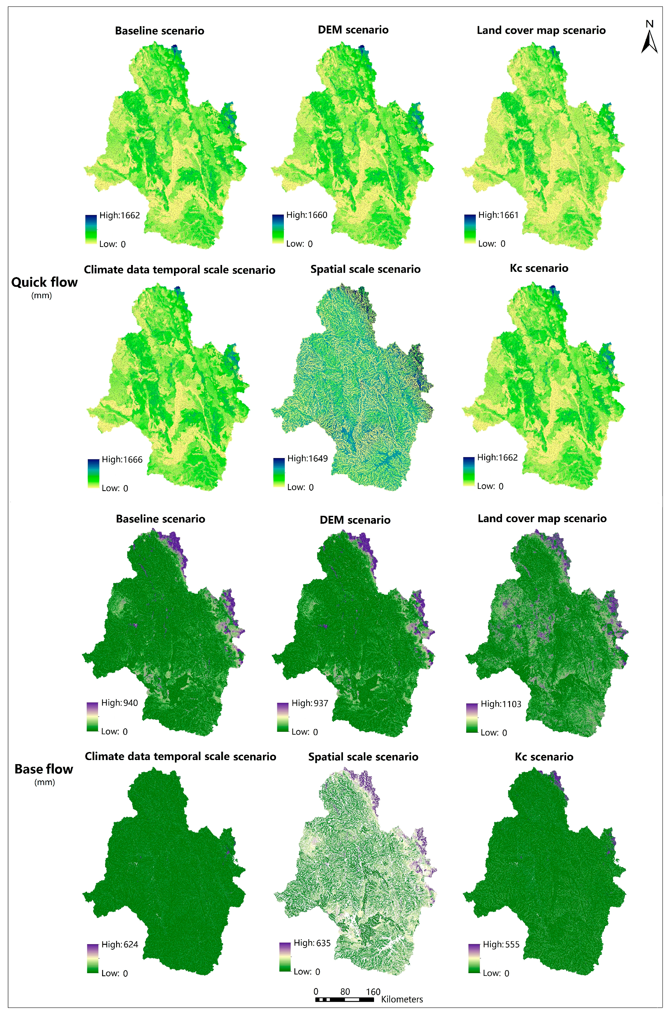
Figure 3.
Pixel value ranges of quick flow & base flow maps (25% percentile to 75% percentile).

Figure 4.
Relative difference between Baseline and uncertainty scenarios.
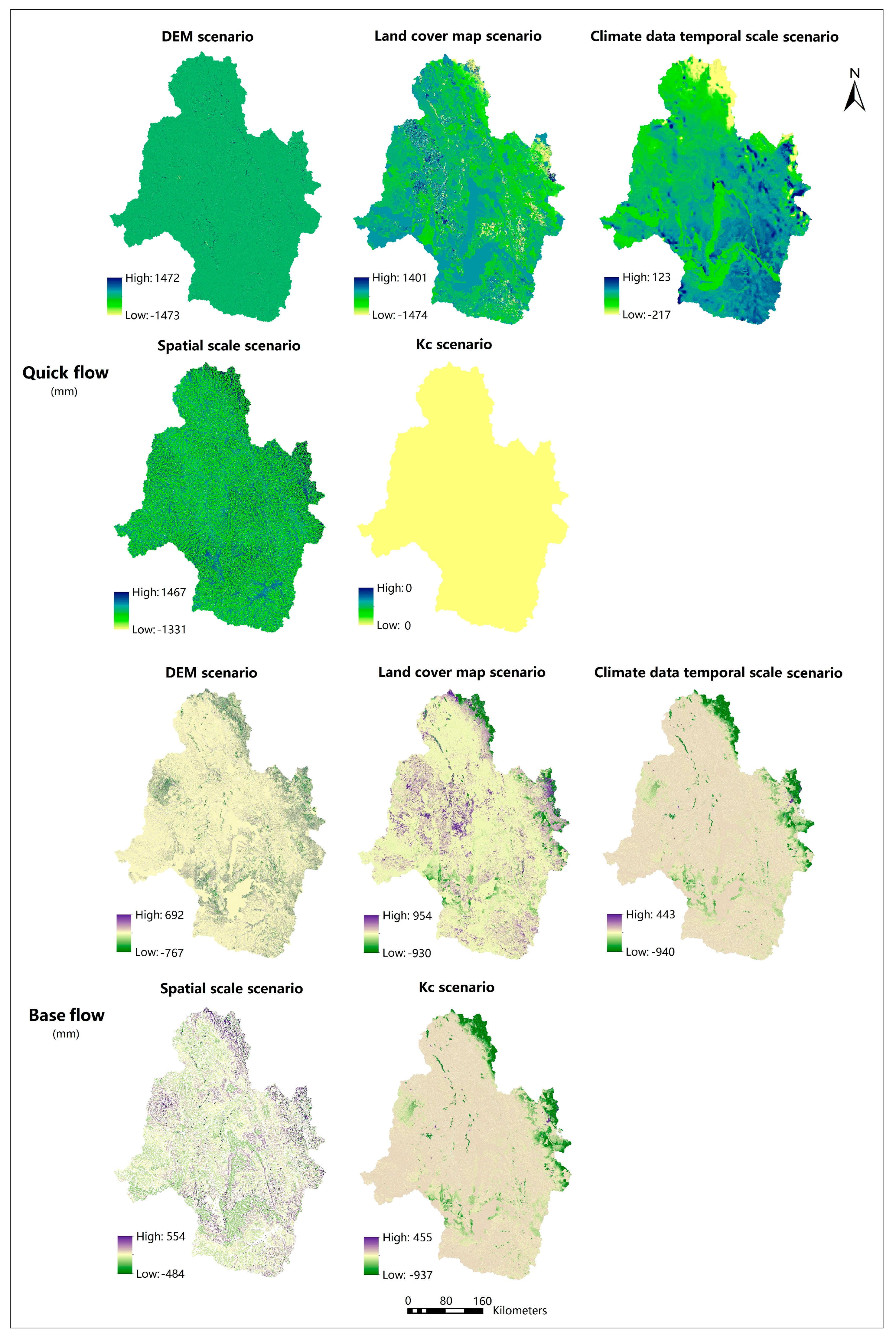
Figure 5.
RVC values of four dominant land use area.
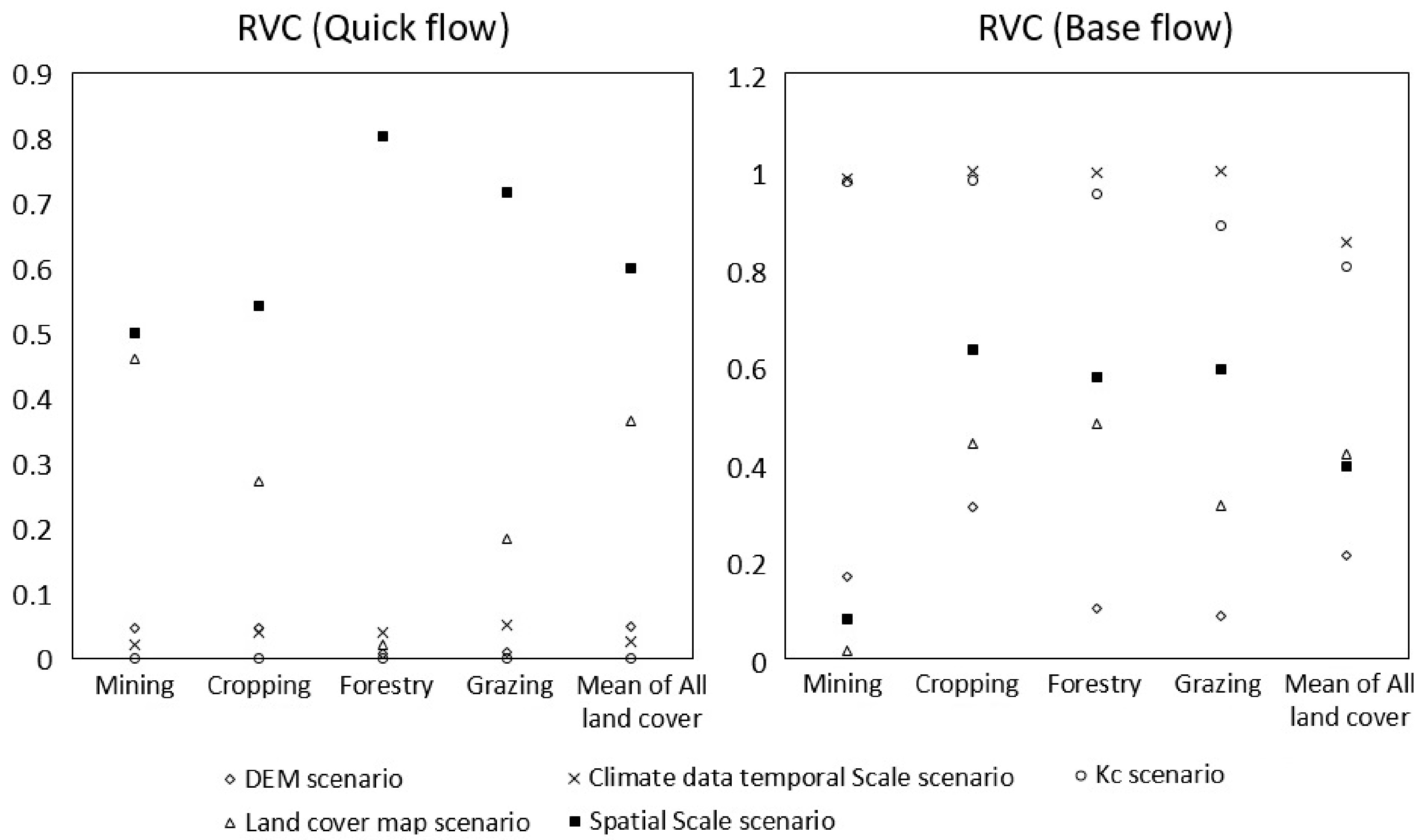
Figure 6.
Catchment-scale annual total water yield.

Table 1.
Inputs and description of Seasonal Water Yield Model.
| Inputs | Model Process | Parameters Description | |
|---|---|---|---|
| Raster layer of monthly precipitation Raster layer of monthly reference evapotranspiration Digital elevation model Raster layer of Land use/land cover (LULC) Raster layer of soil hydrologic groups Vector layer of watershed boundary Biophysical table including CN number and monthly Kc value Rain events table Threshold with 12 values for rain events in each month Threshold flow accumulation | Quick Flow | , | mean rain depth on a rainy day at pixel i on month m number of events at pixel i in month m monthly precipitation for pixel i in month m curve number for pixel i exponential integral function monthly quick flow of stream pixel in month m monthly quick flow of non-stream pixel i in month m annual quick flow of pixel i potential maximum soil moisture retention after runoff begins |
| Local Recharge | = annual local recharge of pixel i annual precipitation of pixel i monthly precipitation of pixel i AET = actual evapotranspiration PET = potential evapotranspiration reference evapotranspiration for month m the available recharge to pixel i pij∈ [0, 1] is the proportion of flow from cell i to j monthly crop factor the fraction of upslope annual available recharge that is available in month m the fraction of the upgradient subsidy that is available for downgradient evapotranspiration = the fraction of pixel recharge that is available to downgradient pixels | ||
| Base Flow | base flow of pixel i cumulative upstream recharge of pixel i j ∈ {cells to which cell i pours} ① for pixels adjacent to stream ② for pixels not adjacent to the stream | ||
Table 2.
Land use and land cover classification for hydrological soil groups (HSG), land types and relevant runoff curve numbers.
Table 2.
Land use and land cover classification for hydrological soil groups (HSG), land types and relevant runoff curve numbers.
| NDLC Classification | QLUMP Classification | ||||||||
|---|---|---|---|---|---|---|---|---|---|
| Land Types | Runoff Curve Number | Land Types | Runoff Curve Number | ||||||
| HSG_A | HSG_B | HSG_C | HSG_D | HSG_A | HSG_B | HSG_C | HSG_D | ||
| Extraction Sites | 81 | 88 | 91 | 93 | Cropping | 70 | 79 | 86 | 90 |
| Inland Waterbodies | 1 | 1 | 1 | 1 | Horticulture | 30 | 55 | 70 | 77 |
| Irrigated Cropping | 70 | 79 | 86 | 90 | Forestry | 36 | 60 | 73 | 79 |
| Rainfed Cropping | 70 | 79 | 86 | 90 | Rural residential | 51 | 68 | 79 | 84 |
| Rainfed Pasture | 49 | 69 | 79 | 84 | Urban residential | 57 | 72 | 81 | 86 |
| Tussock Grasses Open | 49 | 69 | 79 | 84 | Utilities and Services | 89 | 92 | 94 | 95 |
| Hummock Grasses Sparse | 49 | 69 | 79 | 84 | Transport | 83 | 89 | 92 | 93 |
| Tussock Grasses Sparse | 49 | 69 | 79 | 84 | Grazing | 49 | 69 | 79 | 84 |
| Shrubs Closed | 30 | 55 | 70 | 77 | Industrial | 81 | 88 | 91 | 93 |
| Shrubs Sparse | 30 | 55 | 70 | 77 | Bare land | 77 | 86 | 91 | 94 |
| Chenopod Shrubs Sparse | 30 | 55 | 70 | 77 | Water | 1 | 1 | 1 | 1 |
| Trees Closed | 36 | 60 | 73 | 79 | |||||
| Trees Open | 36 | 60 | 73 | 79 | |||||
| Trees Scattered | 36 | 60 | 73 | 79 | |||||
| Trees Sparse | 36 | 60 | 73 | 79 | |||||
Table 3.
Baseline and uncertainty scenarios with alternative spatial data source or modelling scales or parameterization and model tested for a particular scenario in bold.
Table 3.
Baseline and uncertainty scenarios with alternative spatial data source or modelling scales or parameterization and model tested for a particular scenario in bold.
| Uncertainty Types | Scenario Name | Models | Kc Value | Digital Elevation Model (DEM) | Land Use/Land Cover (LULC) | Precipitation and Evapo-Transpiration | Scale Factor |
|---|---|---|---|---|---|---|---|
| - | Baseline scenario | Seasonal water yield model | fPAR derived | SRTM-derived 3 Second DEM of Australia version 1.0 | QLUM land use mapping data | Monthly | 90 m × 90 m per pixel |
| Spatial data sources | DEM | Seasonal water yield model | fPAR derived | DEM derived from contours and drainage of AUSLIG 1:100,000 map | QLUM land use mapping data | Monthly | 90 m × 90 m per pixel |
| Land cover Map | Seasonal water yield model | fPAR derived | SRTM-derived 3 Second DEM of Australia version 1.0 | National Dynamic Land Cover Dataset of Australia | Monthly | 90 m × 90 m per pixel | |
| Modelling scales | Climate data temporal scale | Seasonal water yield model | fPAR derived | SRTM-derived 3 Second DEM of Australia version 1.0 | QLUM land use mapping data | Monthly value calculated as annual value divided by 12 | 90 m × 90 m per pixel |
| Spatial scale | Seasonal water yield model | fPAR derived | SRTM-derived 3 Second DEM of Australia version 1.0 | QLUM land use mapping data | Monthly | ×10 baseline scale | |
| Parameterization and model selection | Annual model | Annual water yield model | fPAR derived | - | QLUM land use mapping data | Annually | 90 m × 90 m per pixel |
| Kc | Seasonal water yield model | Literature based | SRTM-derived 3 Second DEM of Australia version 1.0 | QLUM land use mapping data | Monthly | 90 m × 90 m per pixel |
Table 4.
Inputs and description of Annual Water Yield model.
| Input Data | Model Process | Parameters Description |
|---|---|---|
| Root restricting layer depth Precipitation Plant Available Water Content Average Annual Reference Evapotranspiration Land use/land cover (LULC) Watersheds Sub-watersheds Biophysical Table with annually Kc values and root depth Z (Seasonality factor) | (For vegetated LULC:) (For other LULC:) | Y
= Annual water yield for each pixel = Annual actual evapotranspiration on the pixel x with LULC j Annual precipitation on the pixel x = The ratio of potential evapotranspiration to precipitation = Modified dimensionless ratio of plant accessible water storage to expected precipitation = The volumetric (mm) plant available water content = The reference evapotranspiration from pixel x = Plant (vegetation) evapotranspiration coefficient = Reference evapotranspiration = The evaporation factor for each LULC |
© 2018 by the authors. Licensee MDPI, Basel, Switzerland. This article is an open access article distributed under the terms and conditions of the Creative Commons Attribution (CC BY) license (http://creativecommons.org/licenses/by/4.0/).
Share and Cite
MDPI and ACS Style
Wang, Z.; Lechner, A.M.; Baumgartl, T. Ecosystem Services Mapping Uncertainty Assessment: A Case Study in the Fitzroy Basin Mining Region. Water 2018, 10, 88. https://doi.org/10.3390/w10010088
AMA Style
Wang Z, Lechner AM, Baumgartl T. Ecosystem Services Mapping Uncertainty Assessment: A Case Study in the Fitzroy Basin Mining Region. Water. 2018; 10(1):88. https://doi.org/10.3390/w10010088
Chicago/Turabian StyleWang, Zhenyu, Alex Mark Lechner, and Thomas Baumgartl. 2018. "Ecosystem Services Mapping Uncertainty Assessment: A Case Study in the Fitzroy Basin Mining Region" Water 10, no. 1: 88. https://doi.org/10.3390/w10010088
Note that from the first issue of 2016, this journal uses article numbers instead of page numbers. See further details here.