Sub-Bankfull Flow Frequency versus Magnitude of Flood Events in Outlining Effective Discharges. Case Study: Trotuș River (Romania)


Department of Geography, Faculty of Geography and Geology, Alexandru Ioan Cuza University of Iasi, Iasi RO-700505, Romania
Water 2018, 10(10), 1292; https://doi.org/10.3390/w10101292
Submission received: 25 July 2018
/
Revised: 31 August 2018
/
Accepted: 6 September 2018
/
Published: 20 September 2018
(This article belongs to the Section Hydrology)
Abstract
:Effective discharge, which represents the flow, or range of flows, that transport the most sediment over the long-term, was determined based on the mean daily flow discharge and mean daily suspended sediment discharge recorded between 1994 and 2014 at four gauging stations along the Trotuș River. This study proposes an efficient method for the estimation of effective discharge based on observed values of the suspended sediment load. By employing this method the suspended sediment load is no longer either under- or overestimated as in the cases when the assessment is based on sediment rating curves. The assessment on effective discharge was performed at two distinct levels: for the entire data series during the investigated time spans and, subsequently, for flows less than the bankfull discharge. The effectiveness curves of the suspended sediment transport characteristics revealed highly multimodal characteristics with many peaks, indicating ample ranges for the effective discharges. The main effective discharge corresponded to large flood events, which are typical for the upper end of the discharge range, whereas the secondary effective discharges corresponded to sub-bankfull flows, which are more frequent. The changes that occurred in the channel bed are reflected by the temporal variations in the effective discharge.
1. Introduction
Streamflow is probably the most extensively studied hydrogeomorphic process [1] due to the fact that the volume of water that flows through the channel, sets the scale of the channel [2].
The observation that the shape and size of a stream channel in a state of dynamic equilibrium are the result of a single reference discharge pertains to hydraulic engineers who were building irrigation channels in India in the late 1800s [3]. They noted that these channels can adjust their size depending on the magnitude and frequency of the discharge of water and sediment until a stable configuration is attained [4]. In time, these observations resulted in the development of regime equations which were latter applied to natural streams [5]. By expanding this concept from artificial channels to natural stream channels, the idea has arisen that a single reference discharge or a narrow range of discharges maintain the long-term equilibrium shape and size of the channel, therefore, this discharge could be used as a reference index for the entire series of discharges characteristic for the respective channel. Such index discharges include flows with a specified return period, including the one-in-two year flood (Q2), the bankfull discharge (Qbf) and the effective discharge (Qeff) [6]. Effective discharge is the flow (or narrow range of discharges) which transports the most sediment over time in the stream and, hence, does the most (or greatest proportion of) work in the stream channel [7].
Against this backdrop, the conceptual model introduced by Wolman and Miller [7] has become one of the fundamental paradigms of geomorphology [8]. Subsequent to the publication of this paper, the concept of dominant discharge and its relation to the bankfull and effective discharges have been a hot spot of discussion in fluvial geomorphology for several decades [9], which is evidenced by more than 1800 citations. Wolman and Miller [7] determined the effective discharge of the suspended sediment load in sand-bed rivers with a humid/sub-humid temperate climate and well-vegetated catchments [6,10]. For rivers transporting mostly fine sediment, and assuming a lognormal flow frequency distribution, Wolman and Miller [7] found that the most effective discharge was approximately equal to the bankfull discharge, and has a recurrence interval of 1–2 years [11]. Under the conditions, the effectiveness of the sediment transport was defined as a product of flow frequency and sediment transport by flows of that frequency. Very low flows occur frequently, but typically carry little to no sediment. In turn, very large flows carry considerable amounts of sediment but occur sporadically, therefore, their contribution over time to the total amount of sediment is reduced. Consequently, the effective discharge or the discharge able to transport, on average, the largest suspended sediment load is an intermediate flow [12]. Later on, several studies confirmed the contiguity between effective discharge and bankfull discharge [1,13,14,15], while others pointed out the significant distinctions between the two parameters [16,17,18,19,20,21,22,23]. The studies from the latter category affirm that flow events of a single recurrence interval cannot be considered to be representative of effective or bankfull discharge for all streams. Discharge values are influenced by basin morphology, drainage area, hydrologic regime and sediment transport mode (bedload and suspended sediment load) [6,18,19,20,24,25].
Effective discharge at bankfull stage has been considered to be the key control upon channel formation and/or maintenance [25]. While the effective discharge was initially calculated solely for suspended sediments, several authors [1,6,13,20,26,27] also assessed the bedload or the total load later on. These studies helped introduce the concept of multiple effective discharge or bimodal ‘dominant’ discharge [24]. In geomorphic terms, multiple effective discharges include channel-maintaining [13] and channel-changing discharges [24,28]. The former category comprises higher frequency flows which carry sufficient sediments to maintain channel shape and prevent either aggradation, degradation or vegetative invasion. The latter includes rare floods which exceed a geomorphic threshold, thus prompting significant channel changes [6,13,19,24,27]. Therefore, a distinction is necessary between the effective discharge which refers to “the discharge which transports the most sediment in a stream” and the same term designating “the channel-forming discharge” [12]. In gravel-bed, gravel-bank rivers only the bedload is relevant for channel forming discharges [6,19].
Many streams can exhibit bimodal, multimodal, and heavily skewed flood probability distribution functions [19]. In the case of asymmetric (skewed) effectiveness distributions, a large portion of the total amount of sediments can be carried during flood events at a rare frequency [8,23]. In this context, Vogel et al. [8] question the geomorphic significance of the effective discharge and suggest the use of the half-load discharge (Q1/2) (the discharge above which half the total load is transported) which would be better suited to highlight the effectiveness of rare flood events [12].
Effective discharge frequency is dependent of drainage basin size [28], hydroclimatic regime [1], channel bed, and bank material [26,29], riparian vegetation [10], and channel width and gradient [30]. Initially, Wolman and Miller [7], and later on Andrews [1] and Leopold [31] concluded that the effective discharge can occur once or twice per year. Benson and Thomas [16] established that this discharge is exceeded 12% of the time, or about 44 days per year. Ashmore and Day [18] determined that the effective discharge of the suspended sediment load on the Saskatchewan River ranges from <0.1% to more than 15% of the time. Sichingabula [32] found that Qeff is exceeded between 0.02 and 19.6% of the time or between 7 and 72 days per year. The review published by Ma et al. [25] shows that, in general terms, effective discharge duration occurs between 0.4% and 3% of the time (1.5–11 days per year).
In this paper, long-term (21 years) water discharge and suspended sediment load transport data from the Trotuș River are used to calculate its effective discharge. The assessment of effective discharge was performed based on several methods established in the literature or methods introduced in this study and described in Section 2.3. To highlight multiple effective discharges, their values were also determined for flows below the bankfull discharge.
In summary, the main objectives of this study focus on (i) developing a calculation model for the effective discharge based on observed suspended sediment data instead of data estimated by sediment rating curves; (ii) calculating the effective discharge for the entire data series and the flows below the bankfull discharge; (iii) computing the effective discharge prior to, and after, the 2005 flood events; and (iv) evaluating the relations between effective discharge and stream power.
2. Materials and Methods
This study was based on the use of mean daily flow discharge and suspended sediment. These data were provided by the National Administration “Romanian Waters” Siret Water Branch. The use of high temporal resolution data is typically recommended (e.g., 5-, 15-, 30-, and 60-min interval flow values) [6], particularly for small rivers where the differences between the mean and peak daily discharges are relatively large. In the case of the Trotuș River, the average daily values are regarded as optimal for determining the effective discharge.
2.1. Study Area
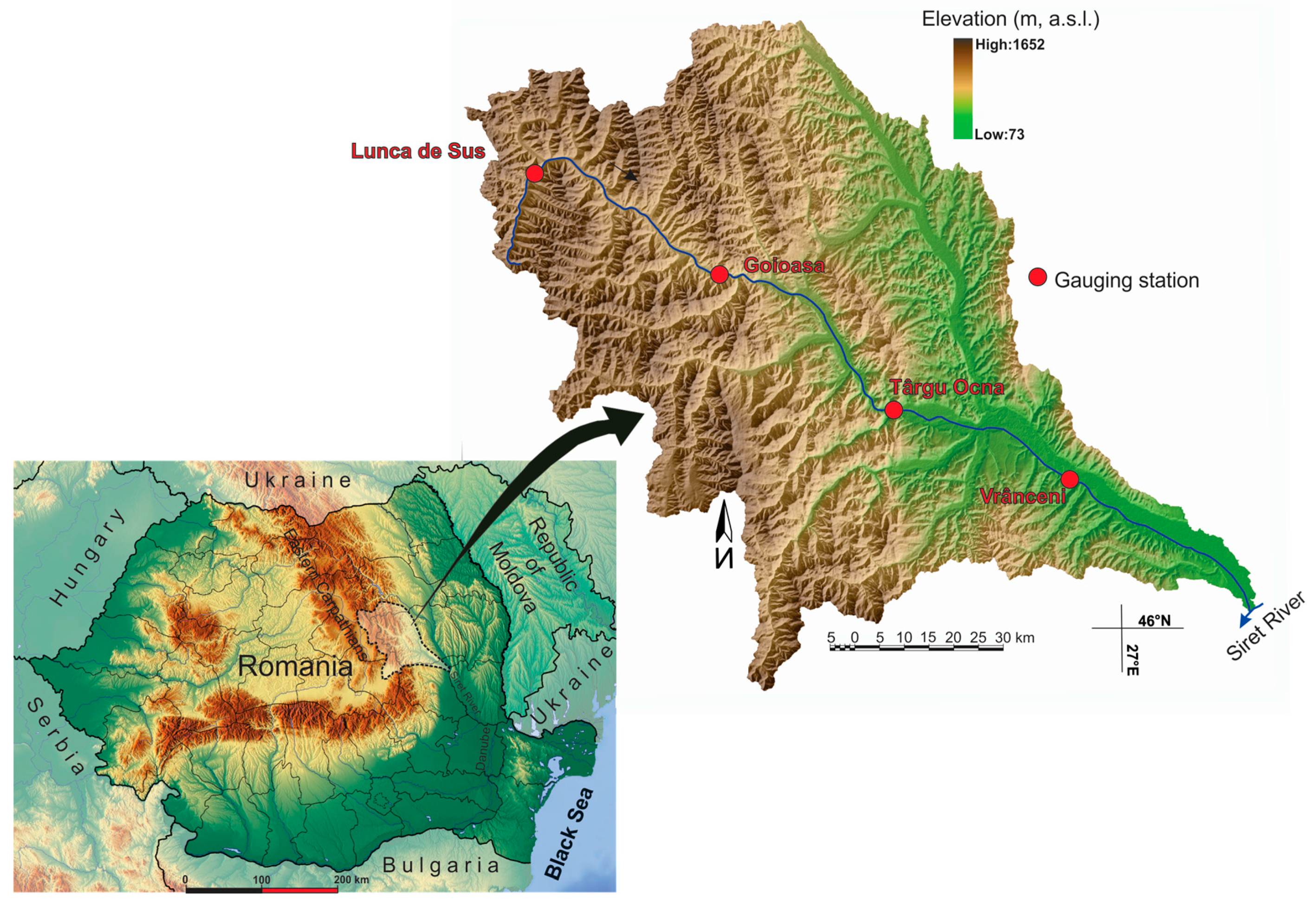
The Trotuș basin is an upper mesoscale mountainous catchment (i.e., 4350 km2) located in the central-eastern part of the Eastern Carpathians (Figure 1). Trotuș River is one of the major tributaries of Siret River, which is, in turn, the largest tributary of the Danube within the Romanian territory.
In terms of lithology, the Carpathian flysch accounts for the largest area of Trotuș drainage basin (~55% of the basin area), ensued by the pericarpathian molasse (~25%), composed of highly erodible rocks such as friable sandstones, clays and marls. The elevation ranges between 73 m above sea level (a.s.l.) at the junction with Siret River and 1672 m a.s.l. at the headwaters. The climate is typical of Carpathian mountainous areas with mean annual precipitation of 720 mm, ranging from 580 in the lowlands to 1150 mm at high altitudes. The share of the precipitation related to the total sum of maximum amounts recorded in 24 h above 100 L/m2 has been rising continually: 8.3% between 1941 and 1960; 30.8% between 1961 and 1980; 47.5% between 1980 and 2000; and 67.7% after 2000 [33]. As regards the land cover/land use, forests, pasturelands and meadows are prevalent in the higher regions of the upper and mid courses, whereas in the lowlands corresponding to the lower course agricultural lands and pastures are dominant. The hydrology of Trotuș River basin is regulated by the pluvio-nival regime, with spring flooding occurring typically in April–May as a result of snowmelt, high precipitation, or the overlapping of both. In June, July, and occasionally extending to August, summer floods can occur as a result of abundant precipitation, reaching very high amplitudes, as was the case with the floods of June–July 2005.
The total length of the Trotuș River is ~160 km. The median diameter (D50) of the bed material along the 160 km amounts to an average of 71.3 mm, with extreme values ranging from 130 mm (in the midcourse) to 20 mm (in the lower course) [34,35]. The mean gradient of the channel ranges between 0.17 mm−1 in the upper course (Lunca de Sus) and 0.018 mm−1 in the lower course (just downstream of Vrânceni) [36]. Based on the average suspended sediment yield (263 t/km2/year) Trotuș drainage basin ranks among the category of rivers with moderate rates from the Romanian Carpathian area [37,38].
In this study, the assessment of the effective discharge was carried out at four gauging stations along the Trotuș River where long-term records of streamflow discharge and suspended sediment load are available. The location and key attributes of these stations are shown in Figure 1 and Table 1, respectively.
2.2. Flow Data Frequency Analysis
Subsequent to the publication of the study by Wolman and Miller [7], a whole array of studies approached the magnitude-frequency analysis (MFA) of flow discharge, which is an essential part of determining the effective discharge [16,39,40]. Although Wolman and Miller [7] suggested that a theoretical probability density function (PDF) can be employed to illustrate the flow regime, it was only after the 1990s that the theoretical MFA approach was perfected [8,19,23,40,41,42].
Three major approaches were used to determine flow frequency [27,43,44], including (i) employing a fixed number of classes (e.g., 25) of equal width and magnitude [16,17]. This method is employed most often but is likely the most criticized [6,11,32] because it depends, to a large extent, on the number of classes. Studies based on the MFA for assessing effective discharge used either an arithmetic scale for flow or a logarithmic scale for building histograms [45]. The following elements should be considered during the process of producing flow-frequency histograms [11,43,45]: the size of the class interval, the number of flow discharge classes, the time period for averaging the discharge, and the length of the period of record. Yevjevich [46] suggested that the size of the class interval for flow discharge should not be larger than SD/4 (where SD represents the standard deviation of the flow for the considered sample), and the number of classes should range between 10 and 25 depending on the sample size. In regard to the length of the period of record, Biedenharn et al. [43] recommended the use of data series 10 to 20 years in length. The second approach is (ii) representing the observed frequency of flow based on the theoretical flow frequency distribution that approximates it, such as the lognormal distribution. This conceptual approach was introduced by Wolman and Miller [7] and later developed by Nash [19]. The application of this method may create particular problems in the case of bimodal, multimodal, heavy-tailed, or heavily skewed flow frequencies [27,41]. The third approach is (iii) computing the amount of sediment transported for each flow class and determining the effective discharge from the steepest point of the cumulative sediment transport curve [26].
2.3. Effective Discharge Computation
The methods involving the use of the flow frequency distribution and a sediment rating curve for the assessment of effective discharge [7,19,47] are regarded as traditional approaches (or deterministic approaches). Moreover, the methods derived from the methodology presented by Crowder and Knapp [11] are considered mean approaches [6,25]. In other articles, the methods for estimating the effective discharge are ranked as class-based (magnitude–frequency) and model-based (analytical) approaches [48].
The estimated value of the effective discharge is strongly influenced by the size and number of class intervals used in the flow frequency analysis [6,9,11,25,27,32,39,49,50]. To remove some of the subjectivity generated by the empirical choice of the size of class interval (CI) or the number of flow discharge classes (N) [25], four different methods were employed for determining the CI and N.
The first method was introduced by Yevjevich [46]. According to the observations by Ma et al. [25] on streams with large flow amplitudes, the criteria proposed by Yevjevich [46] (CI ≤ SD/4 and N = 10–25), Biedenharn et al. [39] and Crowder and Knapp [11] (each class interval should contain at least one flow event) are difficult to apply. For example, at the Vrânceni gauging station, the minimum discharge is 2.2 m3/s, whereas the peak discharge is 2359 m3/s (and the second largest discharge is 1468 m3/s, which results in a difference of 891 m3/s). The SD/4 value is 12.36. Under these circumstances and by considering the previously mentioned recommendations, the number of classes either exceeds 25 or falls below 10 (i.e., four classes, where the effective discharge is placed into the first class, which is also not recommended). To eliminate these drawbacks, Ma et al. [25] proposed to divide flow discharge records into classes by using equal arithmetic intervals corresponding to SD, 0.75 SD, 0.5 SD, and 0.25 SD. Considering the fact that the smaller the size of the class interval is, the more precise the results [9], the class intervals corresponding to 0.25 SD/4, 0.5 SD/4, 0.75 SD/4, and SD/4 were employed for this study.
The second method for determining the CI and N consisted of using kernel density estimation (KDE), which is a non-parametric way to estimate the PDF of a stream flow [23]. The kernel distribution histogram was built using the R statistical software, version 3.5.1. (R is a programming language and free software environment for statistical computing and graphics that is supported by the R Foundation for Statistical Computing). In the case of the two approaches (SD and KDE) employed to estimate the effective discharge of suspended sediment transport, several steps were necessary [14]: (i) determining the flow-frequency distribution, (ii) determining the suspended sediment transport rating curve, and (iii) calculating the effective discharge by multiplying the suspended sediment transport rate for a certain discharge class with the frequency of the respective discharge. The discharge class that accounted for the maximum value of the product was defined as the effective discharge [1].
The third method pertaining to the class-based approach used in this study is the one introduced by Sichingabula [32], which is also known in the literature as the event-based class method (EBM). For this method, the discharge class width is equal in magnitude to the number of decimal places in the maximum value of the data series. For instance, for a maximum discharge ranging between 1 and 9.99 m3/s, the class width is 0.01 m3/s; between 10 and 99.99 m3/s, the class width is 0.1 m3/s; and above 100 m3/s, the class width is 1 m3/s [12,27]. In the case of the Trotuș River, the 0.1 and 1 m3/s class widths were used, which resulted in a total number of classes on the order of hundreds or thousands. For each discharge class, we determined the average magnitude for the class and subsequently used the sediment transport rating curve to evaluate the sediment transport for that class via the class-averaged discharge. The sediment transport rate for each class was multiplied by the flow frequency corresponding to the respective class. The effective discharge was considered to be either the discharge class with the largest value after multiplying the sediment transport and frequency or the peak in the plot of the frequency of sediment transport versus discharge [12].
The fourth method introduces a new way of estimating the effective discharge based on the utilization of real suspended sediment load data instead of the transport rate, which is determined using the suspended sediment rating curve. In fact, this approach is a mixture of the computational versions proposed by Andrews [1]; Sichingabula [32]; Crowder and Knapp [11]; Ma et al. [25]; Tena et al. [50]; and López-Tarazón and Batalla [9]. The discharge classes were established according to the method introduced by Sichingabula [32]. For simplicity, the representative discharge in each class was considered to be the midpoint of the corresponding interval. While Crowder and Knapp [11] employed the average suspended sediment load for each discharge class, Tena et al. [50] and López-Tarazón and Batalla [9] used the real sediment rate for each flow class. In the study by Ma et al. [25], the total suspended sediment load (SSL) transported by the flow discharge of each class interval was calculated by summing the suspended sediment loads of all sample points that fell within the corresponding class interval. The data processing included the following steps: summing the suspended sediment loads for each flow class from the data series, and dividing the value obtained for each class by the frequency (i.e., number of days) of the respective class to yield SSL/day (kg/s). The metric SSL/day (kg/s) was converted into the suspended sediment flux (SSF) (tons/day) [51] for each class. By multiplying the SSF (tons/day) by the flow frequency characteristic for each class, the total suspended sediment load (TSSL) was obtained for each class. TSSL is equivalent to the product of transport rate for suspended sediments and flow frequency, which was yielded via methods based on the sediment rating curve. A much simpler version yielding the same result would imply converting SSL (kg/s) into SSF (tons/day) and summing all of the values obtained for each class, which would determine the real suspended sediment load (RSSL) corresponding to each flow class. The midpoint of the discharge class that transported the largest amount of suspended sediments was considered the effective discharge.
The assessment of effective discharge using an analytical approach was performed according to the indications provided by Nash [19]; Vogel et al. [8]; Goodwin [41]; Quader and Guo [42]; Klonksy and Vogel [23]; and Sholtes et al. [40]. According to this method, the sediment transport mechanics are represented by a power function:
where Qs represents the amount of suspended sediment load (kg/s), Q represents the flow rate (m3/s), and a and b are the fitting parameters.
Qs = aQb
If f(Q) represents the frequency distribution function of the flow series, combining f(Q) with Equation (1) results in the transport effectiveness curve, where the peak is taken as the effective discharge for maximum geomorphic work. The function f(Q) was determined by fitting the logarithmic function to the original distribution of the historical discharge data [48]. According to Nash [19], it was assumed that the daily river discharge (Q) follows a two-parameter lognormal (LN2) distribution, such as:
where μ and σ represent the mean and standard deviation, respectively, of ln(Q).
The effective discharge determined by multiplying the results of Equation (1) with those of Equation (2) can be derived directly by applying Equation (3):
where Qeff (Wolman and Miller) represents the effective discharge based on the Wolman and Miller [7] approach (QeffWM) [8].
Qeff (Wolman and Miller) = exp (μ + (b − 1)σ2)
Vogel et al. [8] questioned the geomorphic significance of effective discharge and preferred instead to use the half-load discharge (Q1/2) (i.e., the discharge above which half of the total load is transported) to summarize the effectiveness of rare floods [12]. Q1/2 was determined according to the methodology presented by Klonksy and Vogel [23].
The effective discharge was estimated at each gauging station using all the approaches described in this section. At each station the following effective discharges were determined: the effective discharge for the entire investigated time frame (1994–1995), the effective flow below the bankfull discharge, and the effective flow prior to and after the floods of 2005.
3. Results
3.1. Flow Frequency
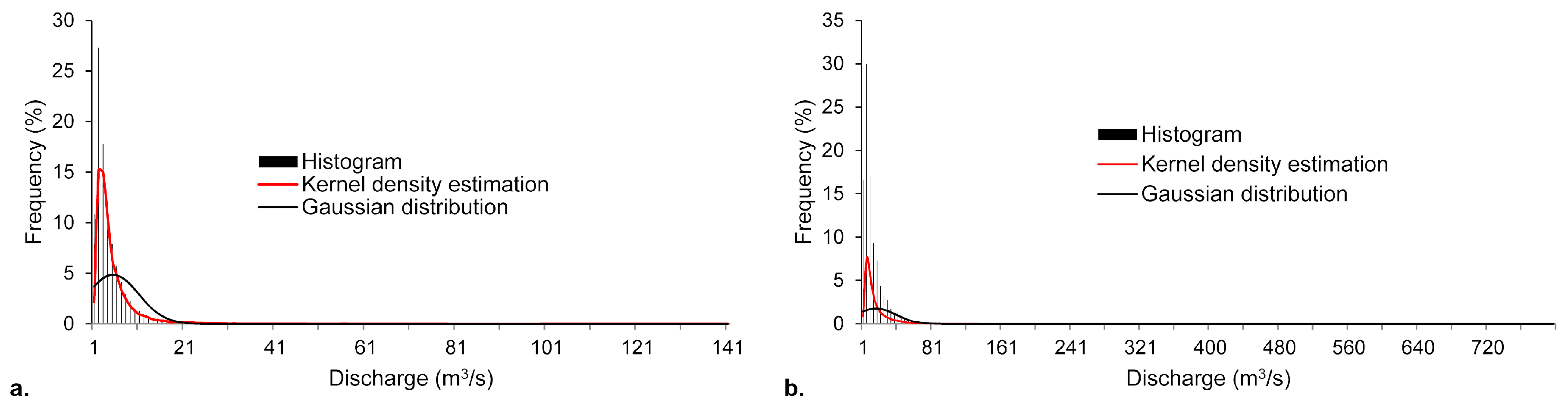
The empirical distribution functions of the discharge time series at all gauging stations along the Trotuș River are heavy-tailed (Figure 2 and Table 2). The heavy-tail properties of the data are characterized by skewness and kurtosis [52].
The kurtosis of the empirical distribution function in a time series provides a quantitative measure of the flow regime variability. While kurtosis values below 3 indicate a normal distribution, values above 3 indicate a type of flow variability where low flows are prevalent. Positive skewness implies that the probability density function is right skewed. Vogel et al. [8] and Klonsky and Vogel [23] showed that in the case of asymmetric (skewed) distributions, much of the total sediment transported may be moved by rare events.
3.2. Suspended Sediment Transport Rating Relations
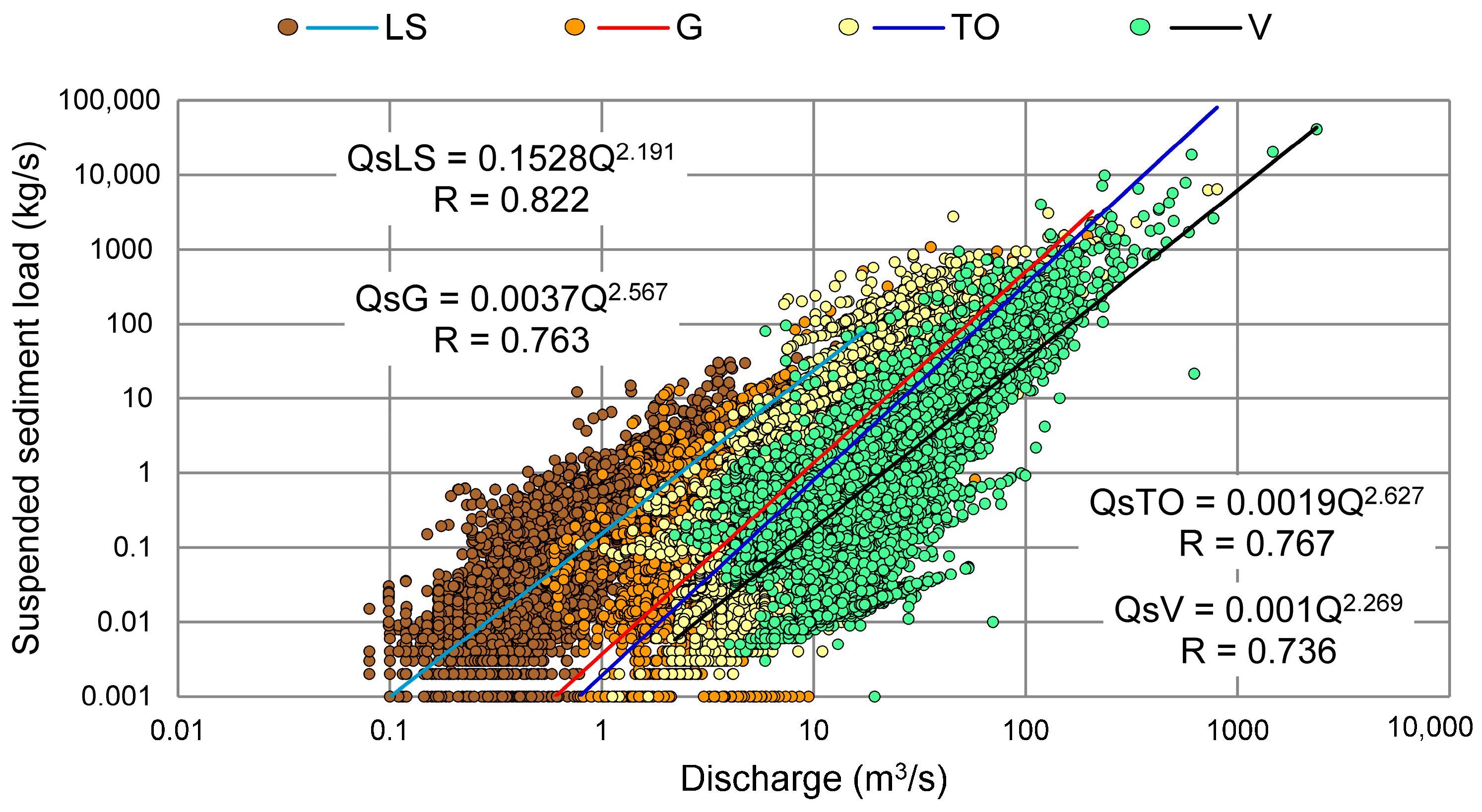
A statistically significant positive relation between discharge and the SSL (Figure 3) can be observed at all gauging stations along the Trotuș River. The values of the b exponent are greater than 1 in all instances (with values ranging between 2.19 and 2.62), which reflects the amount of bed material (i.e., gravel-bed channel) and the fact that discharge must reach a certain threshold to displace the transported alluvium.
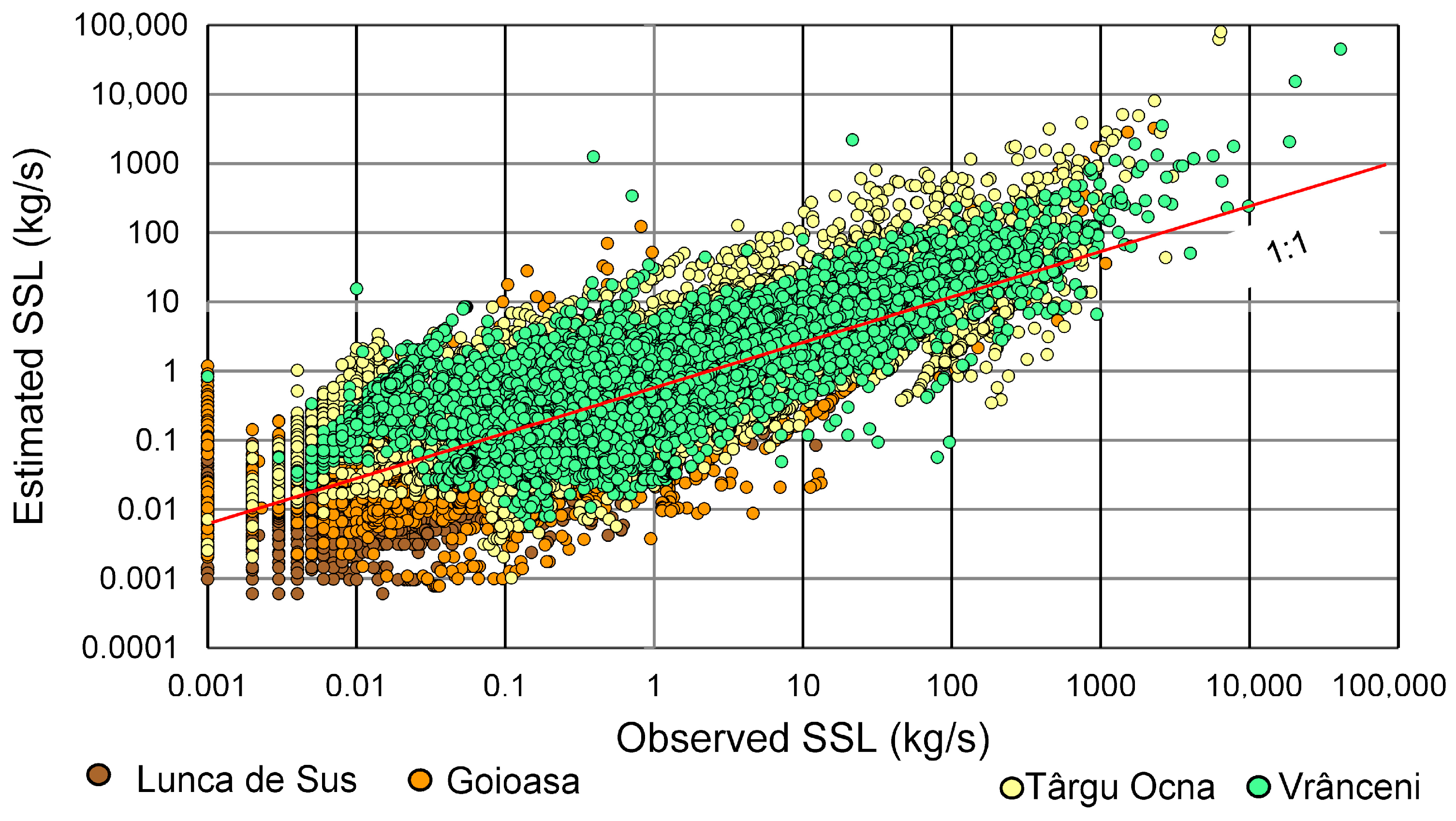
In general, the suspended sediment rating curves tend to underestimate high and overestimate low suspended sediment concentrations [51]. In other instances, it was observed that using a simple transport method developed with a single power function commonly overestimates concentrations with high flow rates, which leads to significant errors when calculating annual loads and the effective discharge [14]. Such differences between the suspended sediment load values and estimated values were also documented in the case of the Trotuș River (Figure 4).
By employing the method described by Horowitz [51], the difference percentages were calculated: −37.8% at Lunca de Sus, −32.7% at Goioasa, +49.1% at Târgu Ocna, and −57.1% at Vrânceni. A minus sign indicates an underprediction, whereas a positive sign indicates an overprediction relative to the measured value.
3.3. Effective Discharge of Suspended Sediment Transport
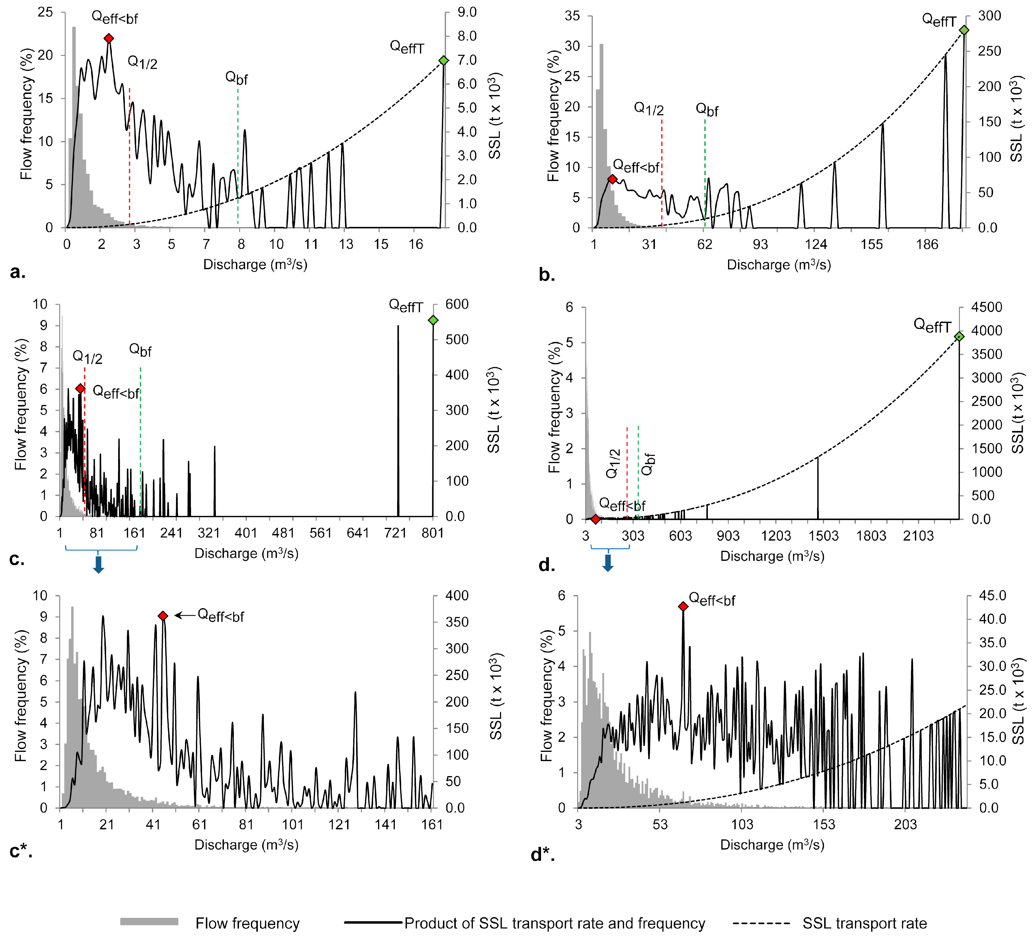
The variability in the effective discharge of the Trotuș River basin from 1994 to 2014 is summarized in Table 3 and Table 4. An overview of the effectiveness curves [47] for the suspended sediment transport characteristics at the four gauging stations along the Trotuș River highlights the highly multimodal characteristics, with many peaks indicating a wide range of effective discharges. With the exception of two instances (i.e., the effective discharges at Lunca de Sus estimated using the SD/4 and KDE methods; Figure 5a), the main effective discharge coincides with large flood events, which typically characterize the upper end of the discharge range. Almost exclusively, the largest measured flood coincides with the effective discharge (see the note in Table 3).
The large amounts of suspended sediments transported during these flood events decrease significantly compared to those transported at moderate flows, such that the latter appears (at first glance) to be almost negligible (Figure 5d). If these peaks indicating large flood events were removed, the presence of several peaks corresponding to moderate flow events would become noticeable. A similar behavior was described by Ma et al. [25] for a group of rivers in a loess region. Biedenharn et al. [39] recommended that isolated peaks in individual classes at the high end of the range for observed discharges are eradicated by reducing the number of classes. By following this recommendation, in the case of the Trotuș River, the number of classes could be as small as 2–4 classes. To eliminate this drawback, an assessment on the effective discharge was performed at two distinct levels: first, for the entire 1994–2014 data series; second, for the flows below bankfull discharge. The bankfull discharge data at the four gauging stations were extracted from Dumitriu [36].
Both categories of effective discharges are important for the evolution of river channels [12,53]. This topic will be resumed later in the paper.
The effective discharge estimated for the entire data series (QeffT) varies depending on significant flood events and is less sensitive to the selected method of computation. In turn, the values of the effective discharge for sub-bankfull flows (Qeff<bf) indicate small differences depending on the method selected for determination, although these are more evident downstream, where flow variability is higher. Overall, however, the differences are negligible and result mostly from the fact that the effective discharge value is considered to be the midpoint of the corresponding interval whereas, at upstream stations (Lunca de Sus and Goioasa), the differences between the Qeff<bf values estimated using the class-based approaches typically range between ±0.1 and 1 m3/s, ±0.4 and 2.6 m3/s at midstream stations (Târgu Ocna) (with one exception), and ±0.2 and as high as 16 m3/s at downstream stations (Vrânceni). At the Vrânceni station, the lowest values were observed for the SD/4 and KDE methods, which is likely because using an optimal kernel density or bin size may mask some information on event frequencies or magnitudes that could be preserved by a slightly less optimal but event-based grouping scheme [27]. The exception mentioned in the case of the Târgu Ocna gauging station refers to the Qeff<bf determined for the 2005–2014 period using the RSSL method, which is lower by nearly 10 m3/s compared to the value estimated using alternative methods. The explanation could reside in the fact that for the 29–30 m3/s flow class, the average suspended solid load was approximately 45 kg/s, whereas in May–July 2006, it amounted to as high as 420 kg/s. Since the three other estimation methods use the sediment rating curve to determine the transport rate, the 29–30 m3/s class was underestimated with respect to the other classes (approximately 40 m3/s).
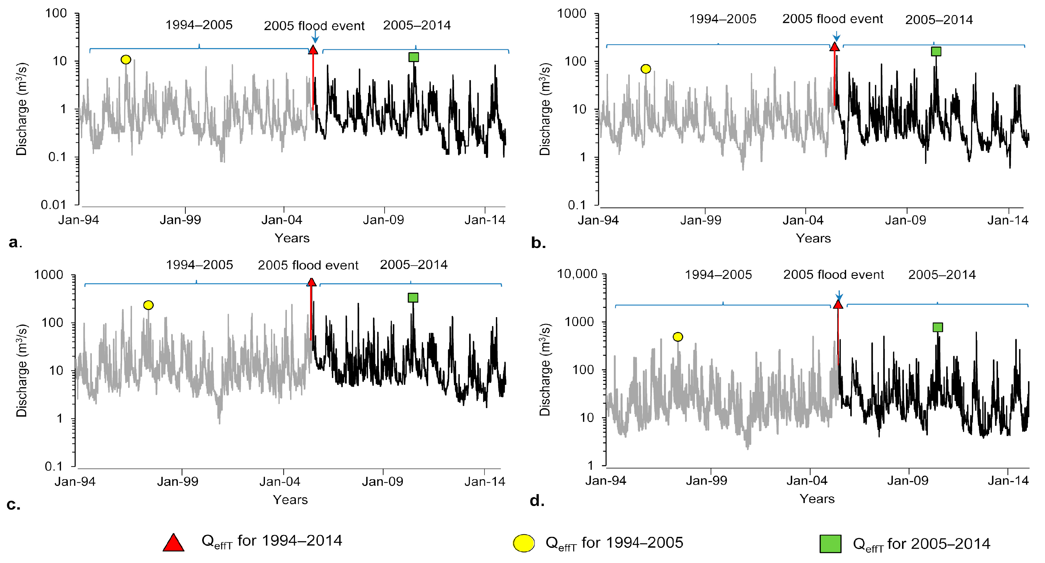
For the 1994–2005 period, QeffT is represented by the flood event of 12–13 July 2005 (Figure 6). The discharges recorded during this time frame are historical peaks, which had an outstanding effect on the river-channel morphology. The peak discharge of 2845 m3/s recorded at Vrânceni station (with a recurrence interval of 625 years) was ranked as the most significant event documented throughout the entire measurement period in the Trotuș drainage basin [36].
From 1994 to 2005 (i.e., the pre-flood event), QeffT was associated (with a few exceptions) with flood events in April 1996 and July 1997. From 2005 to 2014 (i.e., the post-flood event), QeffT corresponded exclusively with the flood event in June 2010.
The values of Qeff<bf were lower from 2005 to 2014 compared with those during the pre-flood event period, which is possibly due to a change in the sediment supply-sediment transport balance [48].
The effective discharge estimated based on the analytical approach (QeffWM) (Table 4) exhibits values similar to those for the Qeff<bf only at Lunca de Sus (1994–2005) and Goioasa (2005–2014), whereas the remaining values are lower. In turn, the Qeff<bf value determined at Târgu Ocna (for the 2005–2014 period using the RSSL method), which is regarded as an exception, is closer to the QeffWM value.
The half-load discharge displays higher values compared to the effective discharge, whereas the Q1/2/Qeff<bf ratio ranges between 0.9 and 4. Thus, it can be stated that QeffT > Q1/2 > Qeff<bf > QeffWM.
4. Discussion
4.1. Influence of Class Interval Assignments
The number of class intervals considered for the assessment of effective discharge can influence, to a significant extent, the effective discharge values and load histograms [11]. In some situations, it has been noted that the effective discharge generally increases with the number of classes [25]. However, this finding cannot be accepted as a general rule because in the majority of cases, the effective discharge does not continuously increase [6,11] or decrease [9,32] with the number of class intervals. In the case of the Trotuș River between 1994 and 2014, an increase (albeit insignificant) in the effective discharge with the number of classes was observed only at Lunca de Sus and Goioasa. At Lunca de Sus, the increase was from 1.9 m3/s (78 class intervals) to 2.1 m3/s (175 class intervals), and at Goioasa, the increase was from 9.8 m3/s (101 class intervals) to 10.5 m3/s (206 class intervals). Since the estimated values of the effective discharge show no significant variations with varying class intervals, the average value was used for comparison (Table 3). Considering the fact that the class midpoint is arbitrarily chosen to represent the effective discharge of that class, and the effectiveness curve is rather irregular, it is more appropriate to use a flow class for the effective discharge [6]. Therefore, the following effective discharge classes were obtained: Lunca de Sus, 1.5–2.5 m3/s; Goioasa, 9.5–10.5 m3/s; Târgu Ocna, 40–45 m3/s; and Vrânceni, 50–65 m3/s.
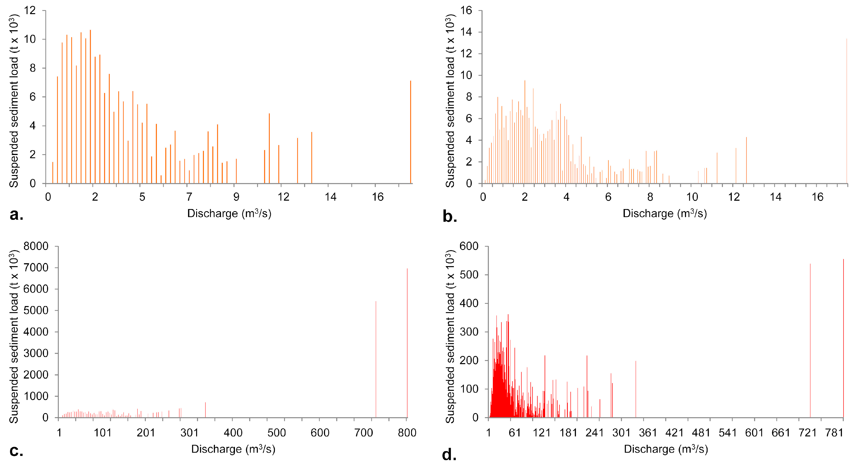
Some differences, depending on the number of classes, have also been observed in suspended solid load histograms. As the number of classes increases, certain variations, in terms of shape (Figure 7) and the total amount of transported sediment, became evident. For instance, at the Lunca de Sus, Goioasa and Târgu Ocna gauging stations, the amounts of suspended sediment estimated using the SD/4, KDE, and EBM methods (with an increasing number of classes) were ca. 1.4 to 1.6 lower compared to the real amounts of suspended sediment transported between 1994 and 2014. At the Vrânceni station, the difference was even higher, with estimated values of 2.2 to 2.4 times lower. Therefore, as the number of classes increases, the total amount of sediment carried throughout the section is underestimated.
Contrary to what Biedenharn et al. [39] stated regarding the fact that a large number of classes would yield abnormal results, in this case, the opposite situation was noted, which corresponded to the observations of López-Tarazón and Batalla [9], who stated that the resulting accuracy increases with a decreasing size of the class interval.
4.2. Duration of Effective Discharge and Recurrence Interval
In many instances, the literature either does not specifically mention the method for estimating the duration of effective discharge, or the estimation was performed using different methods, in which case the results are hardly comparable. In some studies, the determined value represents the flow duration of effective discharge, whereas in other analyses, it stands for the time equal to or exceeding the effective discharge. The former situation refers strictly to the effective discharge class, where the value represents either the duration of the discharge at the upper and lower ends of the class interval [18] or the average flow duration of the effective discharge [9,25,48]. In the latter situation (i.e., the time equals or exceeds the effective discharge), the values of the duration are much larger, as they include all flows higher than or equal to the effective discharge.
The duration of flows pertaining to the classes corresponding to Qeff<bf (which is estimated using both the method described by Ashmore and Day [18] and the average value) varies from 0.9% to 5.02% (1–15 days/year) during the 1994–2014 period, 0.13% to 8.72% (0.9–38.7 days/year) during the 1994–2005 period, and 0.72% to 6.93% (2.6–25.3 days/year) during the 2005–2014 period (Table 5). The duration of QeffT, which accounts for the largest recorded flood discharges, typically ranges between 0.01% and 0.05%. The durations of Qeff<bf determined at the gauging stations along the Trotuș River are within the ranges presented by Ashmore and Day [18], Sichingabula [32], Ma et al. [25], and Roy and Sinha [48]; however, the durations are higher compared to the values obtained by Wolman and Miller [7], Pickup and Warner [17], Andrews [1], and lower than the values determined by López-Tarazón and Batalla [9].
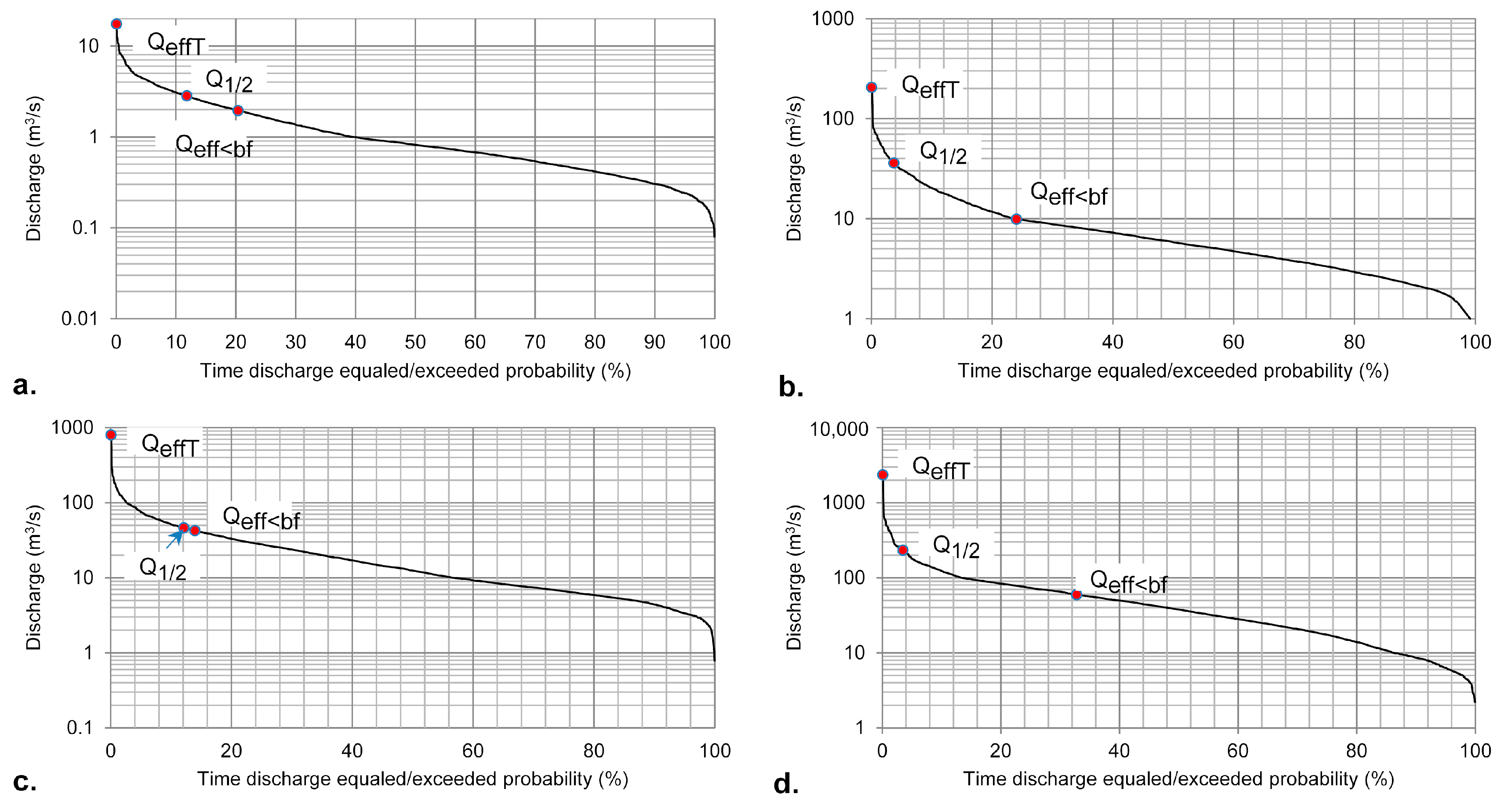
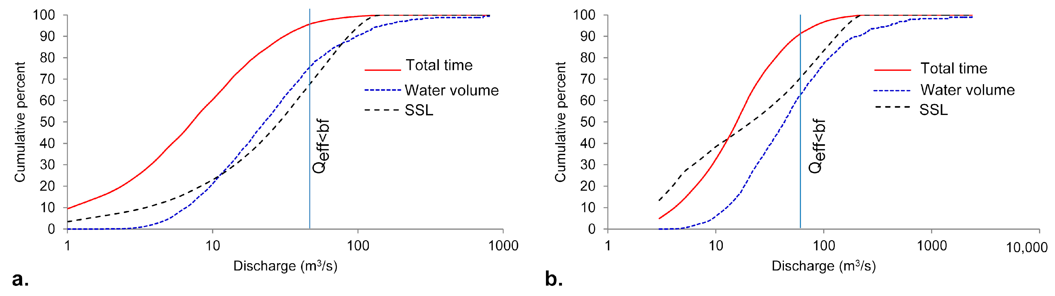
The estimated values of QeffT (1994–2014) had recorded percentages for time equaling or exceeding 0.06% at Lunca de Sus, 0.045% at Goioasa, 0.046% at Târgu Ocna, and 0.08% at Vrânceni. In regard to the times equalling or exceeding Qeff<bf, the values range between 12% and 42% (Figure 8). In general, the values are close to those presented by Klonsky and Vogel [23] for the 15 sites chosen to be representative of all types of rivers throughout the United States.
4.3. Suspended Sediment Transport Rates at Effective and Half-Load Discharges
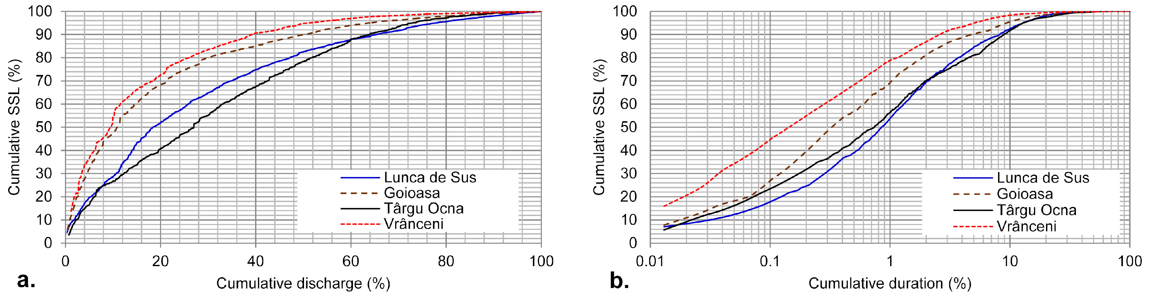
The relation among suspended sediment transport, water flow and the time required to carry out the transport is illustrated by the cumulative curve in Figure 9. The analysis of these curves shows that all of the suspended sediment can be moved with a relatively small portion of annual water yielded during a small part of the year. For example, at the Lunca de Sus gauging station for approximately 7% of the time, Qeff<bf is responsible for the transport of 47% of the total suspended sediment, and it uses 25% of the water flow. At Goioasa, the Qeff<bf requires greater amounts of time (14%) and water (40%) to transport 30% of the total suspended sediment. The respective values are somewhat similar: during an interval ranging between 5% and 9% of the time, Qeff<bf transports 35% and 30% of the total suspended sediment using 27% and 38% of the water discharge, respectively. Therefore, less than 40% of the flow is responsible for effective suspended sediment transport in the Trotuș River.
The percentages of discharge that were needed to transport 10%, 50%, and 90% of the suspended sediments were calculated and are shown in Table 6 and Figure 10. From 1994 to 2014, 10% of the suspended sediment load for all stations was moved by 0.9–2.2% of the total discharge (Figure 10a) and within 0.01–0.025% of the total time (Figure 10b and Table 6). This situation highlights the fact that suspended sediment transport is controlled by flood events. From 2000 to 2014, the percentage of total suspended sediment transported during flood events amounted to 40% at Lunca de Sus, 51% at Goioasa, 38% at Târgu Ocna, and 44% at Vrânceni. Over the course of the same time frame, several years were recorded when the amount of suspended sediment transported during flood events was greater than 80% of the total suspended sediment: Lunca de Sus (2000), Goioasa (2002, 2004, 2005, and 2010), Târgu Ocna (2007) and Vrânceni (2004, 2005, 2007, and 2014) [36]. These events determined the main peak of the effective discharge (QeffT). Half of the total suspended sediment load (the 50th percentile for the total cumulative suspended load) was transported by 10–27% of the total discharge during a time interval ranging between 0.14% and 0.85% of the total time.
In a study carried out in the drainage basin for the Ganga River, Roy and Sinha [48] concluded that in rivers with normal sediment transport capacities, ~90% of the sediment load is transported by 35–60% of the total discharge. At the gauging stations along the Trotuș River two distinct situations were observed. At Goioasa and Vrânceni, 90% of the total suspended sediment load was carried by flows below 50% of the total discharge. At Lunca de Sus and Târgu Ocna, the same percentage of sediment was transported by flows exceeding 60% of the total discharge, thus revealing that the transport capacity varies depending on the hydro-geomorphological traits of the river reach. The results determined for the Trotuș River are partially similar to those reported in the literature. For example, Wolman and Miller [7] showed that in the case of the Colorado River, 50% of the total load is carried by flows equating to 8.5% of the time, while in Rio Puerco, 31% of the total load is transported in just 2.75% of the time. These time percentages correspond to a share of 90% of the total suspended sediment load transported into the Trotuș River. Some of the results published by Roy and Sinha [48] for the transport of 50% of the total suspended sediment load are similar to the results yielded by our study but solely in terms of the percentage of discharge (10–27%) and not in terms of the time percentage (which was 20 to 100 times higher in the case of Ganga River). Typically, in small basins, a large percentage of the total sediment load is moved during rare flood events; therefore, the relation between time and load becomes steeper [6,9,50]. Values close to those recorded at gauging stations along the Trotuș River were reported by Meade and Parker [55] and by López-Tarazón and Batalla [9].
The suspended sediment load corresponding to Q1/2 depends primarily on the surface and particularities of the investigated drainage basin and the runoff characteristics of the study period. Therefore, a variation along the longitudinal profile of the suspended sediment load transported by Q1/2 has been documented, such that from 1994 to 2014, Q1/2 was responsible for the discharge of 155 t × 103 at Lunca de Sus, 1717 t × 103 at Goioasa, 8152 t × 103 at Târgu Ocna, and 13,014 t × 103 at Vrânceni. Similar to the effective discharge, it varies from among streams and longitudinally along a given stream. During the 1994–2005 time frame, Q1/2 had higher values at all stations (with the exception of Goioasa) compared to that during the 2005–2014 period.
4.4. Relation between Effective Discharge and Other Parameters
The mean values of the effective discharge calculated at the sub-bankfull flow (Qeff<bfAvg) were compared to the values of the bankfull discharge (Qbf), mean annual flood (MAF) (the values were taken from Dumitriu [36]), half-load discharge (Q1/2) and mean annual discharge (Qmad) (Table 7).
The values of the Qbf/Qeff<bfAvg ratio range between 3.97 and 6.35 and appear to correlate with the tendencies of degradation, which are more pronounced in the mid- and downstream regions [36]. A series of empirical investigations show that in certain dynamically stable rivers, the effective discharge is relatively close to the bankfull discharge (Qeff ≈ Qbf) [1,26]. However, this situation cannot be generalized [56]. Thus, numerous observations have shown that the relation Qeff ≈ Qbf is valid, particularly for channels in a state of dynamic equilibrium [57]. Qeff < Qbf could offer an indication that the channel is degrading, whereas Qeff > Qbf could point towards aggradation [41]. Values less than 10 for the Qbf/Qeff ratio are not uncommon, as they show an increase in Qbf compared to Qeff due to channel degradation [48].
The value of the Qeff<bfAvg/MAF ratio is less than 1, as the effective discharge is, on average, 50% of the mean annual flood. Wolman and Miller [7] showed that the effective discharge corresponds to the approximate mean annual flood.
At all gauging stations along the Trotuș River, Q1/2 > Qeff<bfAvg, as the values of the ratio range from 0.24 (Vrânceni) to 0.94 (Târgu Ocna). The half-load discharge is typically associated with a higher magnitude and longer return period flow compared to those for the effective discharge [8,23]. In general, Q1/2 is much more frequent and lower than Qbf but less frequent and higher compared to Qmad. Considering the model proposed by Wolman and Miller [7], where Qeff ≈ MAF, it would be expected that Q1/2 ≈ Qeff; however, for strongly skewed effectiveness distributions, Q1/2 and Qeff combined are descriptive of the skew. For Q1/2 > Qeff the effectiveness relation is positively skewed (as documented in the case of the Trotuș River), and for Q1/2 < Qeff, the relation is negatively skewed [27].
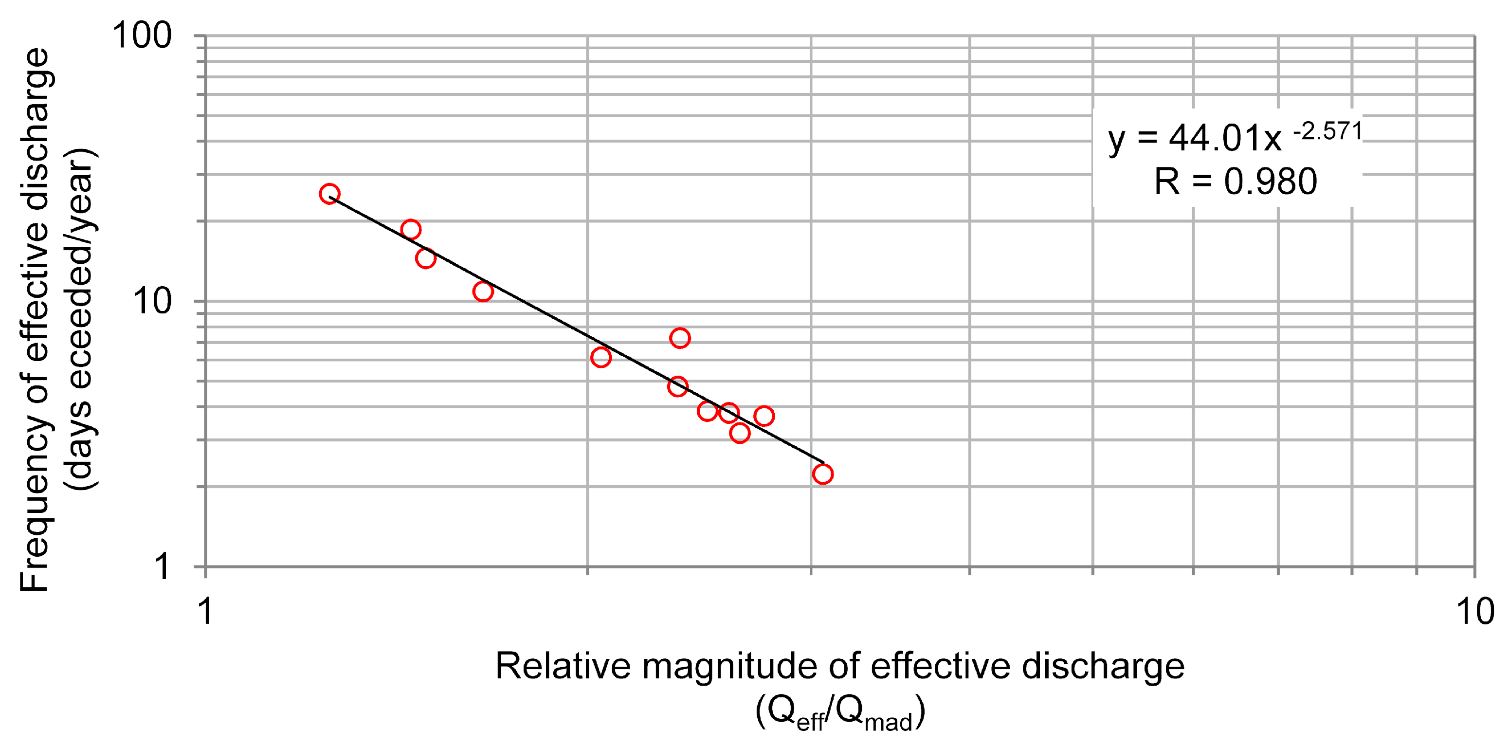
The Qeff/Qmad ratio describes the relative magnitude of the effective discharge. For the Trotuș River, the values of this ratio vary between 1.49 and 2.46. A strong inverse relation between the relative magnitude and frequency of exceedance for effective discharge [27] can also be observed in our study area (Figure 11).
4.5. Temporal Variations in Effective Discharge
The data presented in Table 3 show differences between the effective discharges determined for the two analyzed time frames (1994–2005 and 2005–2014). The Qeff<bf between 2005 and 2014 was 1.2 to 1.7 lower than that in the previous period at three stations (Goioasa, Târgu Ocna, and Vrânceni). At Lunca de Sus, an increase in the Qeff<bf value of 1 m3/s was determined. The decreasing values documented along the mid- and downstream regions can be due to the channel changes that occurred after the flood events of 2005 and 2010. Upstream (Lunca de Sus), channel aggradation became the dominant process, and strong channel degradation was observed in the remaining sectors. In some downstream reaches, the transition from a gravel-bed to gravel bed-bedrock channel occurred as a result of the removal of the armor layer. According to data from the Vrânceni gauging station from 2005 to 2012, the channel bed deepened by 0.85 m [36]. Channel degradation is a major characteristic for most rivers of the Eastern Carpathians [58]. The flood events of 2005 and 2010 transported impressive amounts of suspended sediments, a large part of which was deposited onto the channel bed. On the other hand, suspended sediment availability was strongly dependent upon the stability of the coarse surface layer of the channel bed; when this armor is removed, a significant amount of fine sediments from the subsurface layer becomes accessible to the flow [59,60]. This resulted in an increase in the sources of fine sediments from the channel bed. Such a boost in the sediment supply, particularly the supply of fine sediments, can lead to a decrease in the effective discharge because the channel discharge becomes less capable of transporting excess sediments [48]. This availability of fine sediments is also revealed by higher or sensibly equal amounts of suspended sediments transported at lower Q1/2 values compared to the previous period. For example, at the Târgu Ocna gauging station between 1994 and 2005, Q1/2 was 57.5 m3/s and moved 2704 t × 103 of suspended sediment, whereas from 2005 to 2014, Q1/2 was 36.0 m3/s and transported 4764 t × 103 of suspended sediment (i.e., nearly 1.8 times more than the former period).
In the same context of the temporal variation in effective discharge, an inverse relation was observed between its value and the skewness in the mean daily flow. The Goioasa, Târgu Ocna, and Vrâceni gauging stations experienced increases in the skewness values of the mean daily flow during the 2005–2014 period (from 4.5 to 6.3 on average), which was complemented by a decrease in the effective discharge value. Conversely, at Lunca de Sus, where the skewness in the mean daily flow diminished from 4.1 to 3.8, an increase in effective discharge was documented between 2005 and 2014.
A comparison between the results yielded by our study and the data published by Rădoane and Ichim [61] (i.e., the first and only study to date regarding the effective discharge of a Romanian river—namely, the Trotuș—between 1960 and 1980) reveals that the values are relatively close upstream (at Lunca de Sus and Goioasa), indicating that the channel bed has undergone few changes. However, the effective discharge values determined in our study have nearly double values at the stations located mid- and downstream (Târgu Ocna, and Vrânceni), which results from changes occurring in the channel bed.
4.6. Geomorphic Significance of the Effective Discharge
One of the shortcomings of this study resides in the fact that it only takes into account the suspended sediment load for the assessment of effective discharge; therefore, we are unable to discuss the channel-forming discharge. In this situation, the channel-maintaining discharge may be addressed, at best [6,13,19,24].
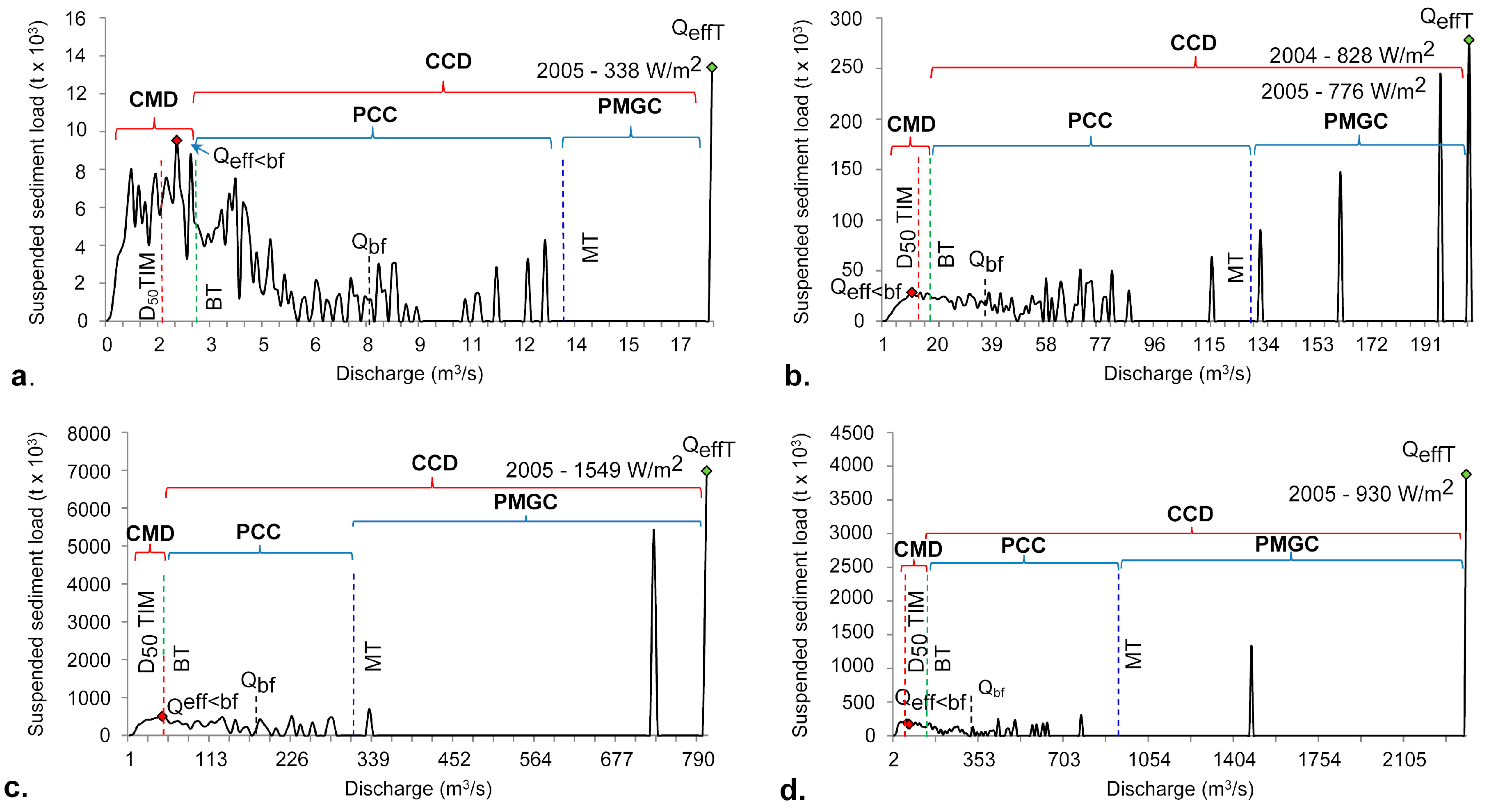
In the Trotuș drainage basin, the contribution of the suspended sediment fraction to the total sediment load ranges from 75 to 90% [62]; nevertheless, the transport of suspended sediments in mountain streams is typically considered to be of secondary geomorphic importance. The data regarding the bed load are rather scarce. Quantification in the field is difficult in many respects, while estimations based on empirical bed-load transport equations yield results that differ by several orders of magnitude depending on the equations used [11]. To compensate (to a certain degree) for the lack of bed load data that would support the delimitation of two types of geomorphically-relevant discharges (i.e., channel-maintaining and channel-changing), a surrogate method was applied. This approach is based on the suggestions made by Crowder and Knapp [11] and Phillips [63] for using stream power to determine the potential thresholds for geomorphic flow. Considering that the thresholds for the transport of various particle sizes or the erosion of various channel materials may be expressed in terms of stream power, in this study, the following specified thresholds were used: (i) critical stream power [64] (regarded as the threshold for D50 incipient motion—D50TIM); (ii) the Brookes threshold (BT) or stability point (35 W/m2), below which the major phase of erosion becomes negligible [65]; and (iii) the Magilligan threshold (MT) (300 W/m2), which is considered the threshold for major morphological adjustments in alluvial channels [66] (Figure 12). Stream power and critical stream power values were taken from Dumitriu [36]. Discharges ranging between the BT and MT can result (under certain conditions) in possible channel changes (PCCs) with a short period of recovery, whereas those exceeding the MT value can generate possible major geomorphic changes (PMGCs) with very long periods of recovery. In this context, discharges above the BT value were considered to be channel-changing discharges (CCD), and those below the BT were included in the channel-maintaining category (CMD). The word “possible” was used because this threshold approach, although attractive, should be used with caution given the complexity of fluvial geomorphic processes.
The discharges corresponding to D50TIM and BT are very close to Qeff<bf in upstream and midstream regions (Figure 12a–c) (at Târgu Ocna, D50TIM and BT correspond to the same discharge (35 m3/s), which is slightly less than Qeff<bf (43 m3/s)). At these stations, Qeff<bf acts similar to a channel-maintaining discharge. Instead, the interval for manifested flows exceeds that of the MT, which could lead to significant channel changes that increase downstream. This finding, along with the peak values of stream power, are in agreement with the field observations made after the flood events of 2005 and 2010 when important channel changes were detected in the mid- and downstream regions [36].
The geomorphic effect of high-magnitude floods has been described in a vast number of papers [67]. These studies discussed the controls of channel responses during flood events. The vast majority of these papers focused mainly on the role of hydraulic variables (e.g., unit stream power and flow duration) [68], whereas others showed that hydraulic variables were insufficient when explaining these changes [69], or their effects differed among streams [70,71]. For example, during the floods generated by Tropical Storm Irene, the minimum threshold of 300 W/m2 was surpassed for 99% of the 60-km Saxons River under study, but the channel widened along considerably smaller reaches [70]. Investigations on streams from the northern Colorado Front Range [71] showed that in channel beds with slope gradients <3% (as is the case with the region upstream of Lunca de Sus), there is the credible potential for substantial channel widening to occur at values >230 W/m2, while at values >700 W/m2, major geomorphic changes can occur. The authors suggest that these thresholds can be utilized for assessing geomorphic hazard potentials via hydraulic modelling. In the case of streams with slopes ≥3% (i.e., most of the length of the Trotuș River), hydraulic variables alone are seldom good predictors of geomorphic change due to variations in bedforms and bed armor, which induce a certain resistance to flow [69,71]. However, the high values of stream power recorded during the 2005 flood event in the mid- and downstream regions (from 830 to 1550 W/m2) were correlated with the field observations, which supported inclusion by comparing these values with QeffT in the channel-forming discharge category. Therefore, depending on the channel characteristics, it is possible that more than one discharge class is responsible for a major part of geomorphic or landform changes [48].
The duration of a flood event can often compensate for the poor predictability of hydraulic variables. In many cases, a better correlation was determined between the magnitude of the channel changes and the flood duration compared to the correlation with hydraulic variables [67]. Thus, in the case of the Trotuș River, it was noted that the flood event of 2010 (lower in magnitude but considerably longer compared to the flood of 2005) generated, in some reaches, many more visible changes than the previous event (2005) when the stream power reached its peak value [36].
5. Conclusions
The relation between flow frequency and magnitude, in terms of outlining effective discharge, is a hot spot in fluvial geomorphology. To reduce the degree of subjectivity generated by the choice of certain flow-class intervals as much as possible, we opted to employ several class-based approaches and analytical methods for the assessment of effective discharge or methods introduced in this study. At all four gauging stations along the Trotuș River, it was observed that the transport efficacy of suspended sediments was generally characterized as highly multimodal, and two types of effective discharges are distinguishable: (1) the main effective discharge (QeffT), which corresponded with rare flows (RI < 20 years in more than 95% of cases) with a magnitude 7- to 82 times greater than that for Qmad; and (2) the sub-bankfull effective discharge (Qeff<bf), which occurs relatively frequently (RI ~ 1.0–1.6 years), with a magnitude 1.5- to 3 times greater than that for Qmad. In regard to the temporal evolution of effective discharges, decreasing factors were documented at Goioasa, Târgu Ocna and Vrânceni, from 1.2 to 1.7, while at Lunca de Sus the value nearly doubled between 2005 and 2014 compared to the previous time frame (1994–2005). The differences were caused by the channel changes generated by the flood events of 2005 and 2010. By plotting hydraulic thresholds with the geomorphic significance on the effectiveness curve of suspended sediment transport, effective discharges corresponding to sub-bankfull flows (Qeff<bf) were ranked as channel-maintaining discharges, whereas the main effective discharges (QeffT) were ranked as channel-changing discharges. The results of this study showcase that the use of calculated values of suspended sediment load, ranked in small class intervals, has a complex relevance, by (1) highlighting more prominently the importance of each flow in terms of sediment transport, and (2) not concealing the real extent of the sediment transport generated by each flood event.
Author Contributions
This paper was the sole work of the author.
Funding
This research received no external funding.
Acknowledgments
This research was partially supported by the Geography Department of the Faculty of Geography and Geology and by CNCSIS—UEFISCSU, project PNII-IDEI number 436/2007. I thanks the anonymous reviewers for their careful reading of our manuscript and their many insightful comments and suggestions. I greatly appreciates the help offered by Florin Obreja, who provided a significant part of the data used in the present study.
Conflicts of Interest
The author declares no conflict of interest.
References
- Andrews, E.D. Effective and bankfull discharges of streams in the Yampa River Basin, Colorado and Wyoming. J. Hydrol. 1980, 46, 311–330. [Google Scholar] [CrossRef]
- Church, M. Channel stability: Morphodynamics and morphology of rivers. In Rivers—Physical, Fluvial and Environmental Processes; Rowinski, P., Radecki-Pawlik, A., Eds.; GeoPlanet-Earth and Planetary Sciences; Springer International Publishing: Basel, Switzerland, 2015; pp. 282–321. ISBN 978-3-319-17719-9. [Google Scholar]
- Inglis, C.C. The behavior and control of rivers and canals. In Research Publication; Central Waterpower Irrigation and Navigation Research Station: Poona, India, 1949; Volume 13, pp. 79–91. [Google Scholar]
- Dollar, E.S.J. Magnitude and frequency controlling fluvial sedimentary systems: Issues, contributions and challenges. IAHR Publ. 2002, 276, 355–362. [Google Scholar]
- Ackers, P. River regime: Research and application. J. Inst. Water Eng. 1972, 26, 257–281. [Google Scholar]
- Lenzi, M.A.; Mao, L.; Comiti, F. Effective discharge for sediment transport in a mountain river: Computational approaches and geomorphological effectiveness. J. Hydrol. 2006, 326, 257–276. [Google Scholar] [CrossRef]
- Wolman, M.G.; Miller, J.P. Magnitude and frequency of forces in geomorphic processes. J. Geol. 1960, 68, 54–74. [Google Scholar] [CrossRef]
- Vogel, R.M.; Stedinger, J.R.; Hooper, R.P. Discharge indices for water quality loads. Water Resour. Res. 2003, 39, 1273. [Google Scholar] [CrossRef]
- López-Tarazón, J.A.; Batalla, R.J. Dominant discharges for suspended sediment transport in a highly active Pyrenean river. J. Soils Sediments 2014, 14, 2019–2030. [Google Scholar] [CrossRef]
- Werritty, A. Short-term changes in channel stability. In Applied Fluvial Geomorphology for River Engineering and Management; Thorne, C.R., Hey, R.D., Newson, M.D., Eds.; Wiley: New York, NY, USA, 1997; pp. 47–65. [Google Scholar]
- Crowder, D.W.; Knapp, H.V. Effective discharge recurrence intervals of Illinois streams. Geomorphology 2005, 64, 167–184. [Google Scholar] [CrossRef]
- Brayshaw, D.D. Bankfull and Effective Discharge in Small Mountain Streams of British Columbia. Ph.D. Thesis, University of British Columbia, Vancouver, BC, Canada, 2012. [Google Scholar]
- Andrews, E.D.; Nankervis, J.M. Effective discharge and the design of channel maintenance flow for gravel-bed rivers. In Natural and Anthropogenic Influences in Fluvial Geomorphology; Costa, J.E., Miller, A.J., Potter, K.W., Wilcock, P.R., Eds.; Geophysical Monograph 89; American Geophysical Union: Washington, DC, USA, 1995; pp. 151–164. [Google Scholar]
- Simon, A.; Dickerson, W.; Heins, A. Suspended-sediment transport rates at the 1.5-year recurrence interval for ecoregions of the United States: Transport conditions at the bankfull and effective discharge? Geomorphology 2004, 58, 243–262. [Google Scholar] [CrossRef]
- Torizzo, M.; Pitlick, J. Magnitude-frequency of bed load transport in mountain streams in Colorado. J. Hydrol. 2004, 290, 137–151. [Google Scholar] [CrossRef]
- Benson, M.A.; Thomas, D.M. A definition of dominant discharge. Bull. Int. Assoc. Sci. Hydrol. 1966, 11, 76–80. [Google Scholar] [CrossRef]
- Pickup, G.; Warner, R.F. Effects of hydrologic regime on magnitude and frequency of dominant discharge. J. Hydrol. 1976, 29, 51–75. [Google Scholar] [CrossRef]
- Ashmore, P.E.; Day, T.J. Effective discharge for suspended sediment transport in streams of the Saskatchewan River Basin. Water Resour. Res. 1988, 24, 864–870. [Google Scholar] [CrossRef] [Green Version]
- Nash, D.B. Effective sediment-transporting discharge from magnitude frequency analysis. J. Geol. 1994, 102, 79–95. [Google Scholar] [CrossRef]
- Whiting, P.J.; Stamm, J.F.; Moog, D.B.; Orndorff, R.L. Sediment-transporting flows in headwaters streams. Geol. Soc. Am. Bull. 1999, 111, 450–466. [Google Scholar] [CrossRef]
- Gomez, B.; Coleman, S.E.; Sy, V.W.K.; Peacock, D.H.; Kent, M. Channel change, bankfull and effective discharges on a vertically accreting, meandering, gravel-bed river. Earth Surf. Process. Landf. 2007, 32, 1–5. [Google Scholar] [CrossRef]
- Quader, A.; Guo, Y.P.; Stedinger, J.R. Analytical estimation of effective discharge for small southern Ontario streams. Can. J. Civ. Eng. 2008, 35, 1414–1426. [Google Scholar] [CrossRef]
- Klonsky, L.; Vogel, R. Effective measures of “effective” discharge. J. Geol. 2011, 119, 1–14. [Google Scholar] [CrossRef]
- Phillips, J.D. Geomorphological impacts of flash flooding in a forested headwater basin. J. Hydrol. 2002, 269, 236–250. [Google Scholar] [CrossRef]
- Ma, Y.; Huang, H.Q.; Xu, J.; Brierley, G.J.; Yao, Z. Variability of effective discharge for suspended sediment transport in a large semi-arid river basin. J. Hydrol. 2010, 388, 357–369. [Google Scholar] [CrossRef]
- Emmett, W.W.; Wolman, M.G. Effective discharge and gravel-bed rivers. Earth Surf. Process. Landf. 2001, 26, 1369–1380. [Google Scholar] [CrossRef]
- Hassan, M.A.; Brayshaw, D.; Alila, Y.; Andrews, E. Effective discharge in small formerly glaciated mountain streams of British Columbia: Limitations and implications. Water Resour. Res. 2014, 50, 4440–4458. [Google Scholar] [CrossRef] [Green Version]
- Wolman, M.G.; Gerson, R. Relative scales of time and effectiveness of climate in watershed geomorphology. Earth Surf. Process. Landf. 1978, 3, 189–208. [Google Scholar] [CrossRef]
- Nolan, K.M.; Lisle, T.E.; Kelsey, H.M. Bankfull discharge and sediment transport in a northwestern California. In Erosion and Sedimentation in the Pacific Rim; IAHS Press: Wallingford, UK, 1987; Volume 165, pp. 439–449. [Google Scholar]
- Pitlick, J. Response of Coarse Bed Rivers to Large Floods in Colorado and California. Ph.D. Thesis, Colorado State University, Fort Collins, CO, USA, 1988. [Google Scholar]
- Leopold, L.B. A View of the River; Harvard University Press: Cambridge, MA, USA, 1994; ISBN 978-06-7401-845-7. [Google Scholar]
- Sichingabula, H.M. Magnitude-frequency characteristics of effective discharge for suspended sediment transport, Fraser River, British Columbia, Canada. Hydrol. Process. 1999, 13, 1361–1380. [Google Scholar] [CrossRef]
- Pleşoianu, D.; Olariu, P. Monitoring data proving hydroclimatic trends in Siret hydrographic area. Present Environ. Sustain. Dev. 2010, 4, 327–338. [Google Scholar]
- Dumitriu, D. Sediment System of the Trotuş Drainage Basin; Universităţii Press: Suceava, Romania, 2007; ISBN 978-973-666-237-9. (In Romanian) [Google Scholar]
- Dumitriu, D.; Condorachi, D.; Niculiţă, M. Downstream variation in particle size: A case study of the Trotuş River, Eastern Carpathians (Romania). Analele Universității Oradea Geografie 2011, 21, 222–232. [Google Scholar]
- Dumitriu, D. Geomorphic effectiveness of floods on Trotuș river channel (Romania) between 2000 and 2012. Carpathian J. Earth Environ. Sci. 2016, 11, 181–196. [Google Scholar]
- Dumitriu, D. Source area lithological control on sediment delivery ratio in Trotuş drainage basin (Eastern Carpathians). Geografia Fisica Dinamica Quaternaria 2014, 37, 91–100. [Google Scholar]
- Dumitriu, D.; Rădoane, M.; Rădoane, N. Sediment sources and delivery. In Landform Dynamics and Evolution in Romania; Rădoane, M., Vespremeanu-Stroe, A., Eds.; Springer: New York, NY, USA, 2017; pp. 629–654. ISBN 978-3-319-32589-7. [Google Scholar]
- Biedenharn, D.S.; Copeland, R.R.; Thorne, C.R.; Soar, P.J.; Hey, R.D.; Watson, C.C. Effective Discharge Calculation: A Practical Guide; Technical Rep. No. ERDC/CHL TR-00-15; U.S. Army Corps of Engineers: Washington, DC, USA, 2000. [Google Scholar]
- Sholtes, J.; Werbylo, K.; Bledsoe, B. Physical context for theoretical approaches to sediment transport magnitude-frequency analysis in alluvial channels. Water Resour. Res. 2014, 50, 7900–7914. [Google Scholar] [CrossRef] [Green Version]
- Goodwin, P. Analytical solutions for estimating effective discharge. J. Hydraul. Eng. 2004, 130, 729–738. [Google Scholar] [CrossRef]
- Quader, A.; Guo, Y.P. Relative importance of hydrological and sediment-transport characteristics affecting effective discharge of small urban streams in Southern Ontario. J. Hydrol. Eng. 2009, 14, 698–710. [Google Scholar] [CrossRef]
- Biedenharn, D.S.; Thorne, C.R.; Soar, P.J.; Hey, R.D.; Watson, C.C. Effective discharge calculation guide. Int. J. Sediment Res. 2001, 16, 445–459. [Google Scholar]
- Soar, P.J.; Thorne, C.R. Design discharge for river restoration. In Stream Restoration in Dynamic Fluvial Systems; Simon, A., Bennett, S.J., Castro, J.M., Eds.; Geophysical Monograph Series 194; Wiley: Hoboken, NJ, USA, 2011; pp. 123–149. [Google Scholar]
- Soar, P.J.; Thorne, C.R. Channel Restoration Design for Meandering Rivers; ERDC/CHL CR-01-1; U.S. Army Corps of Engineers: Washington, DC, USA, 2001. [Google Scholar]
- Yevjevich, V. Probability and Statistics in Hydrology; Water Resources Publications: Fort Collins, CO, USA, 1972. [Google Scholar]
- Doyle, M.W.; Stanley, E.H.; Strayer, D.L.; Jacobson, R.B.; Schmidt, J.C. Effective discharge analysis of ecological processes in streams. Water Resour. Res. 2005, 41, 1–16. [Google Scholar] [CrossRef]
- Roy, N.G.; Sinha, R. Effective discharge for suspended sediment transport of the Ganga River and its geomorphic implication. Geomorphology 2014, 227, 18–30. [Google Scholar] [CrossRef]
- Quader, A. Analytical estimation of the effective discharge of small urban streams. Ph.D. Thesis, McMaster University, Hamilton, ON, Canada, 2007. [Google Scholar]
- Tena, A.; Batalla, R.J.; Vericat, D.; Lopez-Tarazon, J.A. Suspended sediment dynamics in a large regulated river over a 10-year period (the lower Ebro, NE Iberian Peninsula). Geomorphology 2011, 125, 73–84. [Google Scholar] [CrossRef]
- Horowitz, A.J. An evaluation of sediment rating curves for estimating suspended sediment concentrations for subsequent flux calculations. Hydrol. Process. 2003, 17, 3387–3409. [Google Scholar] [CrossRef]
- Sen, A.K.; Niedzielski, T. Statistical characteristics of river flow variability in the Odra River Basin, Southwestern Poland. Pol. J. Environ Stud. 2010, 19, 387–397. [Google Scholar]
- Bourke, M.C. Suspended sediment concentrations and the geomorphic effect of sub-bankfull flow in a central Australian stream. In The Structure, Function and Management Implications of Fluvial Sedimentary Systems; Dyer, F.J., Thoms, M.C., Olley, J.M., Eds.; Publication IAHS 276; IAHS Press: Wallingford, UK, 2002. [Google Scholar]
- Sholtes, J.S. On the Magnitude and Frequency of Sediment Transport in Rivers. Ph.D. Thesis, Colorado State University, Fort Collins, CO, USA, 2015. [Google Scholar]
- Meade, R.H.; Parker, R.S. Sediment in rivers of the United States. In U.S. Geological Survey Water-Supply Paper 2275, National Water Summary; U.S. Government Printing Office: Washington, DC, USA, 1984; pp. 49–60. [Google Scholar]
- Klasz, G.; Reckendorfer, W.; Gutknecht, D. Morphological aspects of bankfull and effective discharge of gravel-bed rivers and changes due to channelization. In Proceedings of the 9th International Symposium on Ecohydraulics, Vienna, Austria, 17–21 September 2012. [Google Scholar]
- Copeland, R.R.; Biedenharn, D.S.; Fischenich, J.C. Channel-Forming Discharge; Technical Note ERDC/CHL CHETN-VIII-5; U.S. Army Corps of Engineers: Washington, DC, USA, 2000. [Google Scholar]
- Rădoane, M.; Obreja, F.; Cristea, I.; Mihailă, D. Changes in the channel-bed level of the eastern Carpathian rivers: Climatic vs. human control over the last 50 years. Geomorphology 2013, 193, 91–111. [Google Scholar] [CrossRef]
- Diplas, P.; Parker, G. Deposition and removal of fines in gravel-bed streams. In Dynamics of Gravel-Bed Rivers; Billi, P., Hey, R.D., Thorne, C.R., Tacconi, P., Eds.; John Wiley & Sons: Chichester, UK, 1992; pp. 313–329. ISBN 0-471-92976-X. [Google Scholar]
- Lenzi, M.A.; Mao, L.; Comiti, F. Interannual variation of suspended sediment load and sediment yield in an alpine catchment. Hydrol. Sci. 2003, 48, 899–915. [Google Scholar] [CrossRef] [Green Version]
- Rădoane, M.; Ichim, I. The concept of geomorphic effectiveness and its significance in the sediment transport in the Trotuş River Basin. Lucrările Simpozionului Provenienţa şi Efluenţa Aluviunilor 1986, 1, 275–282. (In Romanian) [Google Scholar]
- Olariu, P.; Obreja, F.; Obreja, I. Some aspects concerning the sediment yield in the Trotus drainage basin and the lower Siret sector, during major floods from 1991 and 2005. Analele Universităţii Ştefan cel Mare Suceava Geografie 2009, XVIII, 93–104. (In Romanian) [Google Scholar]
- Phillips, J.D. Hydrologic and geomorphic flow thresholds in the Lower Brazos River, Texas, USA. Hydrol. Sci. J. 2015, 60, 1631–1648. [Google Scholar] [CrossRef]
- Williams, G.P. Paleohydrological methods and some examples from Swedish fluvial environments. I. Cobble and boulder deposits. Geogr. Ann. 1983, 65, 227–243. [Google Scholar] [CrossRef]
- Brookes, A. River Channelization in England and Wales: Downstream Consequences for the Channel Morphology and Aquatic Vegetation. Ph.D. Thesis, University of Southampton, Southampton, UK, 1983. [Google Scholar]
- Magilligan, F.J. Thresholds and the spatial variability of flood power during extreme floods. Geomorphology 1992, 5, 373–390. [Google Scholar] [CrossRef]
- Costa, J.E.; O’Connor, J.E. Geomorphically effective floods. In Natural and Anthropogenic Influences in Fluvial Geomorphology; Costa, J.E., Miller, A.J., Potter, K.W., Wilcock, P., Eds.; Geophysical Monograph Series 89; American Geophysical Union: Washington, DC, USA, 1995; pp. 45–56. ISBN 978-0-875-90046-9. [Google Scholar]
- Magilligan, F.J.; Buraas, E.M.; Renshaw, C.E. The efficacy of streampower and flow duration on geomorphic responses to catastrophic flooding. Geomorphology 2015, 228, 175–188. [Google Scholar] [CrossRef]
- Surian, N.; Righini, M.; Lucìa, A.; Nardi, L.; Amponsah, W.; Benvenuti, M.; Borga, M.; Cavalli, M.; Comiti, F.; Marchi, L.; et al. Channel response to extreme floods: Insights on controlling factors from six mountain rivers in Northern Apennines, Italy. Geomorphology 2016, 272, 78–91. [Google Scholar] [CrossRef]
- Buraas, E.M.; Renshaw, C.E.; Magilligan, F.J.; Dade, W.B. Impact of reach geometry on stream channel sensitivity to extreme floods. Earth Surf. Process. Landf. 2014, 39, 1778–1789. [Google Scholar] [CrossRef]
- Yochum, S.E.; Sholtes, J.S.; Scott, J.A.; Bledsoe, B.P. Stream power framework for predicting geomorphic change: The 2013 Colorado Front Range flood. Geomorphology 2017, 292, 178–192. [Google Scholar] [CrossRef]
Figure 1.
Location of the study area in the Eastern Carpathians and locations of discharge and sediment gauging stations; data from these stations were used for this study.
Figure 1.
Location of the study area in the Eastern Carpathians and locations of discharge and sediment gauging stations; data from these stations were used for this study.

Figure 2.
Comparisons between histograms and kernel density approximations of discharge data for the Trotuș River. (a) Goioasa; (b) Târgu Ocna.
Figure 2.
Comparisons between histograms and kernel density approximations of discharge data for the Trotuș River. (a) Goioasa; (b) Târgu Ocna.

Figure 3.
Relationship between water discharge and suspended sediment load at the four gauging stations along the Trotuș River (1994–2014).
Figure 3.
Relationship between water discharge and suspended sediment load at the four gauging stations along the Trotuș River (1994–2014).

Figure 4.
Scatter plot of relationship between observed and estimated suspended load at the four gauging stations along the Trotuș River (1994–2014).
Figure 4.
Scatter plot of relationship between observed and estimated suspended load at the four gauging stations along the Trotuș River (1994–2014).

Figure 5.
Examples of estimation of QeffT, Qeff<bf and Q1/2 for suspended sediment transport using various methods: (a) Lunca de Sus—KDE; (b) Goioasa—SD/4; (c,c*) Târgu Ocna—RSSL; (d,d*) Vrânceni—EBM.
Figure 5.
Examples of estimation of QeffT, Qeff<bf and Q1/2 for suspended sediment transport using various methods: (a) Lunca de Sus—KDE; (b) Goioasa—SD/4; (c,c*) Târgu Ocna—RSSL; (d,d*) Vrânceni—EBM.

Figure 6.
Association of QeffT with peak/maximum values. (a) Lunca de Sus; (b) Goioasa; (c) Târgu Ocna; (d) Vrânceni.
Figure 6.
Association of QeffT with peak/maximum values. (a) Lunca de Sus; (b) Goioasa; (c) Târgu Ocna; (d) Vrânceni.

Figure 7.
Load histograms for Trotuș River at Lunca de Sus: (a) SD/4 method—78 classes; (b) EBM method—175 classes and Târgu Ocna; (c) KDE method—200 classes; and (d) RSSL method—800 classes.
Figure 7.
Load histograms for Trotuș River at Lunca de Sus: (a) SD/4 method—78 classes; (b) EBM method—175 classes and Târgu Ocna; (c) KDE method—200 classes; and (d) RSSL method—800 classes.

Figure 8.
QeffT, Qeff<bf and Q1/2 equalled/exceeded probability. (a) Lunca de Sus; (b) Goioasa; (c) Târgu Ocna; (d) Vrânceni.
Figure 8.
QeffT, Qeff<bf and Q1/2 equalled/exceeded probability. (a) Lunca de Sus; (b) Goioasa; (c) Târgu Ocna; (d) Vrânceni.

Figure 9.
Cumulative suspended sediment-water-time curves during 1994–2014. (a) Târgu Ocna; (b) Vrânceni.
Figure 9.
Cumulative suspended sediment-water-time curves during 1994–2014. (a) Târgu Ocna; (b) Vrânceni.

Figure 10.
Cumulative percentage of suspended sediment load versus discharge (a) and time duration (b) (period 1994–2014).
Figure 10.
Cumulative percentage of suspended sediment load versus discharge (a) and time duration (b) (period 1994–2014).

Figure 11.
Relation between frequency of effective discharge and relative magnitude of effective discharge.
Figure 11.
Relation between frequency of effective discharge and relative magnitude of effective discharge.

Figure 12.
Differentiation between channel-maintaining and channel-changing discharges based on specific thresholds of stream power. (a) Lunca de Sus; (b) Goioasa; (c) Târgu Ocna; (d) Vrânceni.
Figure 12.
Differentiation between channel-maintaining and channel-changing discharges based on specific thresholds of stream power. (a) Lunca de Sus; (b) Goioasa; (c) Târgu Ocna; (d) Vrânceni.


Table 1.
Hydrologic parameters associated with each station.
| Station Name | DRM | A | S | Qavg | Qmin | Qmax | Red | Qs | Qsmax | SSY |
|---|---|---|---|---|---|---|---|---|---|---|
| Lunca de Sus (LS) | 146 | 88 | 0.02 | 0.8 | 0.1 | 17.5 | 218.8 | 0.5 | 0.2 | 167.5 |
| Goioasa (G) | 106 | 781 | 0.07 | 6.6 | 0.5 | 206 | 377.3 | 5.2 | 2.3 | 209.4 |
| Târgu Ocna (TO) | 69 | 2091 | 0.05 | 15.5 | 0.8 | 800 | 1012.7 | 24.6 | 6.4 | 371.3 |
| Vrânceni (V) | 37 | 4092 | 0.03 | 28.9 | 2.2 | 2359 | 1067.4 | 39.3 | 41.0 | 302.9 |
Note: DRM—distance to the river mouth (km); A—drainage area (km2); S—slope (m/m); Qavg—mean daily discharge (1994–2014) (m3/s); Qmin—minimum mean daily discharge (1994–2014) (m3/s); Qmax—maximum mean daily discharge (1994–2014) (m3/s); Red—ratio of maximum mean daily discharge to minimum mean daily discharge; Qs—mean daily suspended sediment load (1994–2014) (kg/s); Qsmax—maximum mean daily suspended sediment load (1994–2014) (kg/s); SSY—suspended sediment yield (t/km2/year).
Table 2.
Basic statistics of daily flow time series (1994–2014) from Trotuș River.
| Station | Standard Deviation | Coefficient of Variation | Skewness | Kurtosis |
|---|---|---|---|---|
| Lunca de Sus | 0.91 | 1.09 | 4.66 | 40.41 |
| Goioasa | 8.24 | 1.24 | 7.86 | 122.79 |
| Târgu Ocna | 22.54 | 1.45 | 12.69 | 341.84 |
| Vrânceni | 49.46 | 1.71 | 19.90 | 760.29 |
Table 3.
Effective discharges for suspended sediment transport in Trotuș River using traditional and mean approaches.
Table 3.
Effective discharges for suspended sediment transport in Trotuș River using traditional and mean approaches.
| Station | Period | SD/4 | KDE | EBM | RSSL | Qeff<bfAvg | RI Qeff<bfAvg | ||||
|---|---|---|---|---|---|---|---|---|---|---|---|
| QeffT | Qeff<bf | QeffT | Qeff<bf | QeffT | Qeff<bf | QeffT | Qeff<bf | ||||
| LS | A | 17.6 a | 1.9 | 17.4 | 1.9 | 17.5 | 2.1 | 17.5 | 2.1 | 2.0 | 1.3 |
| B | 8.4 b | 1.0 | 10.7 | 1.1 | 6.1 m | 1.0 | 8.4 n | 1.0 | 1.0 | 1.0 | |
| C | 12.2 c | 2.1 | 12.1 | 1.9 | 12.2 | 1.9 | 12.1 | 2.1 | 2.0 | 1.3 | |
| G | A | 205.4 d | 9.8 | 205.3 | 9.9 | 206.0 | 10.5 | 205.5 | 9.5 | 9.9 | 1.0 |
| B | 73.3 e | 16.3 | 73.0 | 17.5 | 73.3 | 16.6 | 73.5 | 17.5 | 17.0 | 1.1 | |
| C | 159.9 f | 10.5 | 159.8 | 9.7 | 160.9 | 10.5 | 160.5 | 9.5 | 10.1 | 1.0 | |
| TO | A | 798.1 g | 43.1 | 798.2 | 42.8 | 800.0 | 41.5 | 800.5 | 44.1 | 42.8 | 1.6 |
| B | 234.0 h | 43.9 | 231.0 | 46.1 | 233.0 | 46.5 | 128.0 o | 45.5 | 45.5 | 1.7 | |
| C | 333.2 i | 42.2 | 330.7 | 43.7 | 333.0 | 41.6 | 332.5 | 29.5 | 39.2 | 1.5 | |
| V | A | 2359.7 j | 54.7 | 2354.6 | 50.4 | 2359.0 | 66.5 | 2358.5 | 65.5 | 59.3 | 1.2 |
| B | 487.5 k | 72.5 | 483.4 | 69.9 | 487.0 | 70.7 | 235.5 p | 70.5 | 70.9 | 1.4 | |
| C | 766.5 l | 52.5 | 764.2 | 46.8 | 769.0 | 49.5 | 604.0 q | 49.5 | 49.6 | 1.1 | |
Note: A—1994–2014; B—1994–2005; C—2005–2014; QeffT—effective discharge calculated for the entire data series (m3/s); Qeff<bf—effective discharge calculated for flows below Qbf (m3/s); Qeff<bfAvg—average effective discharge calculated for flows below Qbf (m3/s); RI Qeff<bfAvg—recurrence interval of Qeff<bfAvg (years); SD/4—Standard Deviation—Yevjevich method [46]; KDE—Kernel Density Estimation; EBM—Event-Based class Methodology; RSSL—Real Suspended Sediment Load; a—flood event of 12 July 2005 (17.5 m3/s); b—flood event of 26 April 1996 (10.8 m3/s); c—flood event of 21 June 2010 (12.2 m3/s); d—flood event of 12 July 2005 (206 m3/s); e—flood event of 26 April 1996 (73.3 m3/s); f—flood event of 26 June 2010 (160.1 m3/s); g—flood event of 13 July 2005 (800.2 m3/s); h—flood event of 28 July 1997 (233 m3/s); i—flood event of 26 June 2010 (333 m3/s); j—flood event of 13 July 2005 (2359 m3/s); k —flood event of 28 July 1997 (487 m3/s); l—flood event of 26 June 2010 (769 m3/s); m—flood event of 30 March–6 April 2000 (~6 m3/s); n—flood event of 23–29 April 1996 and 22–24 July 2001 (> 8 m3/s); o—flood event of 14 June 1998 and 8 August 2002 (128 m3/s); p—flood event of 27 August 1997 (236 m3/s); q—flood event of 26 May 2012 (607 m3/s).
Table 4.
Effective discharges and half-load discharge for suspended sediment transport in the Trotuș River using analytical approaches.
Table 4.
Effective discharges and half-load discharge for suspended sediment transport in the Trotuș River using analytical approaches.
| Station | Period | QeffWM | b | μ | σ | QeffWM TE | RI QeffWM | Q1/2 | RI Q1/2 | SSY at Q1/2 |
|---|---|---|---|---|---|---|---|---|---|---|
| (m3/s) | (%) | (years) | (m3/s) | (years) | (t × 103) | |||||
| LS | A | 1.2 | 2.19 | −0.513 | 0.779 | 33.8 | 1.1 | 2.9 | 1.4 | 154.6 |
| B | 1.2 | 2.21 | −0.504 | 0.748 | 38.0 | 1.1 | 2.7 | 1.4 | 77.8 | |
| C | 1.3 | 2.17 | −0.526 | 0.812 | 31.4 | 1.1 | 2.6 | 1.4 | 66.9 | |
| G | A | 12.0 | 2.57 | 1.552 | 0.767 | 19.6 | 1.0 | 36.0 | 1.4 | 1716.8 |
| B | 11.8 | 2.82 | 1.552 | 0.708 | 19.7 | 1.0 | 31.0 | 1.4 | 674.2 | |
| C | 11.6 | 2.34 | 1.545 | 0.823 | 20.2 | 1.0 | 37.0 | 1.4 | 861.2 | |
| TO | A | 30.8 | 2.63 | 2.293 | 0.835 | 21.7 | 1.3 | 45.6 | 1.7 | 8152.3 |
| B | 29.0 | 2.55 | 2.301 | 0.827 | 23.8 | 1.3 | 57.5 | 1.8 | 2703.8 | |
| C | 33.1 | 2.68 | 2.387 | 0.812 | 20.0 | 1.4 | 36.0 | 1.4 | 4763.1 | |
| V | A | 46.0 | 2.27 | 2.944 | 0.834 | 43.0 | 1.1 | 242.0 | 2.8 | 13,014.1 |
| B | 50.0 | 2.54 | 2.910 | 0.806 | 40.0 | 1.1 | 180.0 | 2.3 | 5369.7 | |
| C | 40.0 | 1.97 | 2.981 | 0.856 | 47.8 | 1.0 | 177.0 | 2.3 | 4830.9 |
Table 5.
Average flow duration of Qeff<bf (effective discharges are shown in Table 3).
Table 5.
Average flow duration of Qeff<bf (effective discharges are shown in Table 3).
| Station | Period | SD/4 | KDE | EBM | RSSL | ||||
|---|---|---|---|---|---|---|---|---|---|
| (%) | Days/Year | (%) | Days/Year | (%) | Days/Year | (%) | Days/Year | ||
| LS | A | 1.74 | 6.3 | 1.68 | 6.1 | 0.90 | 3.3 | 0.90 | 3.3 |
| B | 8.72 | 38.7 | 6.90 | 25.2 | 5.25 | 19.2 | 6.91 | 25.2 | |
| C | 2.23 | 8.1 | 2.57 | 9.4 | 1.27 | 4.6 | 1.88 | 6.9 | |
| G | A | 5.02 | 18.3 | 4.75 | 17.3 | 2.79 | 10.1 | 3.38 | 12.3 |
| B | 1.33 | 4.9 | 0.97 | 3.6 | 1.33 | 4.9 | 0.52 | 1.9 | |
| C | 6.49 | 23.7 | 6.93 | 25.3 | 3.16 | 11.5 | 3.83 | 14.0 | |
| TO | A | 1.74 | 6.3 | 1.41 | 5.1 | 0.59 | 2.1 | 0.31 | 1.1 |
| B | 0.83 | 3.0 | 1.05 | 3.8 | 0.33 | 1.2 | 0.13 | 0.9 | |
| C | 1.10 | 4.0 | 1.39 | 5.1 | 0.72 | 2.6 | 1.01 | 3.7 | |
| V | A | 1.90 | 6.9 | 4.12 | 15.0 | 0.47 | 1.7 | 0.26 | 1.0 |
| B | 1.00 | 3.6 | 1.50 | 5.5 | 0.50 | 1.8 | 0.50 | 1.8 | |
| C | 3.64 | 13.3 | 6.36 | 23.2 | 0.95 | 3.5 | 0.95 | 3.5 | |
Table 6.
Cumulative suspended sediment load in given percentage of time and by percentage of total discharge (period 1994–2014).
Table 6.
Cumulative suspended sediment load in given percentage of time and by percentage of total discharge (period 1994–2014).
| Station | 10% of Total Cumulative Suspended Load | 50% of Total Cumulative Suspended Load | 90% of Total Cumulative Suspended Load | |||
|---|---|---|---|---|---|---|
| % of Time | % of Total Discharge | % of Time | % of Total Discharge | % of Time | % of Total Discharge | |
| LS | 0.025 | 1.8 | 0.85 | 18 | 8.0 | 65 |
| G | 0.017 | 0.9 | 0.32 | 11 | 4.7 | 50 |
| TO | 0.024 | 2.2 | 0.74 | 27 | 8.8 | 64 |
| V | 0.010 | 1.0 | 0.14 | 10 | 2.5 | 39 |
Table 7.
Ratios of parameters computed.
| Station | Period | Qbf/Qeff<bfAvg | Qeff<bfAvg/MAF | Qeff<bfAvg/Q1/2 | Qeff<bfAvg/Qmad | Q1/2/Qmad |
|---|---|---|---|---|---|---|
| Lunca de Sus | 1994–2014 | 4.05 | 0.49 | 0.69 | 2.36 | 3.42 |
| Goioasa | 1994–2014 | 6.35 | 0.35 | 0.28 | 1.49 | 5.42 |
| Târgu Ocna | 1994–2014 | 3.97 | 0.63 | 0.94 | 2.76 | 2.93 |
| Vrânceni | 1994–2014 | 5.48 | 0.40 | 0.24 | 2.05 | 8.37 |
© 2018 by the author. Licensee MDPI, Basel, Switzerland. This article is an open access article distributed under the terms and conditions of the Creative Commons Attribution (CC BY) license (http://creativecommons.org/licenses/by/4.0/).
Share and Cite
MDPI and ACS Style
Dumitriu, D. Sub-Bankfull Flow Frequency versus Magnitude of Flood Events in Outlining Effective Discharges. Case Study: Trotuș River (Romania). Water 2018, 10, 1292. https://doi.org/10.3390/w10101292
AMA Style
Dumitriu D. Sub-Bankfull Flow Frequency versus Magnitude of Flood Events in Outlining Effective Discharges. Case Study: Trotuș River (Romania). Water. 2018; 10(10):1292. https://doi.org/10.3390/w10101292
Chicago/Turabian StyleDumitriu, Dan. 2018. "Sub-Bankfull Flow Frequency versus Magnitude of Flood Events in Outlining Effective Discharges. Case Study: Trotuș River (Romania)" Water 10, no. 10: 1292. https://doi.org/10.3390/w10101292
Note that from the first issue of 2016, this journal uses article numbers instead of page numbers. See further details here.