Verification and Correction of the Hydrologic Routing in the Soil and Water Assessment Tool


1
Institute of Hydrology and Water Resources Management, Universität Hannover, Appelstraße 9A, 30167 Hannover, Germany
2
Thuy Loi University, 175 Tay Son, Hanoi, Vietnam
*
Author to whom correspondence should be addressed.
Water 2018, 10(10), 1419; https://doi.org/10.3390/w10101419
Submission received: 10 September 2018
/
Revised: 4 October 2018
/
Accepted: 9 October 2018
/
Published: 10 October 2018
(This article belongs to the Section Hydrology)
Abstract
:The Soil and Water Assessment Tool (SWAT) is one of the most widely used eco-hydrological models. SWAT has been undergoing constant changes since its development. However, compartment review and testing of SWAT, especially the hydrologic routing functions, are comparably limited. In this study, the daily hydrologic routing subroutines of different SWAT versions were reviewed and tested using a well observed segment of the Weser River located in Germany. Results show several problems with the routing subroutines of SWAT. The variable storage subroutine of SWAT (Revision 664) does not transform the stream flow. Unphysical results could be obtained with the variable storage routing of SWAT (Revision 528). The Muskingum subroutine of SWAT (Revisions 664 and 528) overestimates daily channel evaporation (resulting in a bias of up to 6.3% in streamflow in our case studies) and underestimates daily transmission losses. Simulated results show that the timing and shape of flood waves, as well as the volume of low flows, could be improved with a corrected Muskingum subroutine. Based on the results of this study, we suggest that the SWAT user community review their existing SWAT models to see how the aforementioned issues will affect their methods, findings, and conclusions.
1. Introduction
Flood routing is predicting the timing and magnitude of a flood wave at a downstream point of a reach from the known data at an upstream point [1]. It plays an important role in flood forecasting, reservoir design, and flood control. In semi-distributed hydrologic models, simplified hydrologic routing methods are often applied for flood routing instead of hydraulic methods. Hydrologic routing also serves as a basic function for sediment and nutrient routing [2]. The parameters of hydrologic models are often calibrated against observed streamflow, sediment, and/or nutrient yields. Therefore, having a robust and well-tested hydrologic routing function in hydrologic models is important.
The Soil and Water Assessment Tool (SWAT) is a conceptual semi-distributed hydrologic model used to predict the effect of land use management practices on water, sediment, and nutrient yield [2,3]. SWAT has been undergoing constant changes since its development [4]. SWAT has been tested and applied worldwide [4,5,6]. However, compartment verification of SWAT is limited, especially regarding its hydrologic routing functions.
With SWAT, users can select either the variable storage method [7] or the Muskingum method [8,9] for hydrologic routing [3]. There have been some modifications to the routing functions in SWAT, e.g., [10,11]. Kim and Lee [10] suggested implementing a nonlinear storage equation obtained by coupling continuity and Manning’s equations, to avoid underestimation of peak flows and false signals during the recession period with the Muskingum used in SWAT. Pati et al. [11] replaced the Muskingum used in SWAT with the variable parameter McCarthy–Muskingum to enhance channel routing. In the official SWAT revisions (https://swat.tamu.edu/), however, the model uses the two aforementioned methods [7,8,9] for hydrologic routing. Despite this, our preliminary studies show that there is a significant difference in terms of simulated streamflow between the two methods and between the same method in different SWAT versions (as shown in Section 4).
The main objective of this study is to explain the differences in simulated streamflow and motivate users of the model to draw more attention to the hydrologic routing processes. This study provides (1) an overview into the technical aspects of the two hydrologic routing methods used in SWAT, (2) an insight to the code implementation of these concepts in different SWAT revisions, and (3) an improvement of the SWAT hydrologic routing functions. A case study for a well observed segment of the Weser River, Germany, is used as a verification example.
2. Theoretical Background
2.1. Variable Storage Method
The variable storage method is based on the continuity equation [7]:
where I (m/s) and O (m/s) are the inflow and outflow rate for a river reach, respectively, t (s) is the time, S (m) is the storage. In discrete form, Equation (1) becomes
where the subscripts “1” and “2” refer to the start and end of the routing time interval t (s), respectively. Equation (2) can be rearranged to have the following form:
where is the average inflow rate during the time interval. The travel time, T (s), is calculated as follows:
Equation (3) can be rewritten using Equation (4) to obtain the relation between the storage coefficient and the travel time:
where C is the storage coefficient:
The condition C ≤ 1 must be satisfied to avoid unphysical results.
2.2. Muskingum Method
The Muskingum method is based on the continuity equation (Equation (1) and (2)) and the empirical linear storage equation [9,12]:
where S (m) is the total storage in channel, K (s) is the storage constant, X (-) is a weighting factor, ranging from 0 to 0.5, and I (m/s) and O (m/s) are inflow and outflow rate. From Equations (2) and (9), the following relation can be obtained:
where
where , , and are coefficients. To avoid numerical instability, the following condition must be satisfied:
3. Hydrologic Routing with SWAT
In this section, the daily variable storage and Muskingum method in SWAT2000, SWAT2005, SWAT2009 (Revision 528), and SWAT2012 (Revision 664) are reviewed. The source code of these SWAT versions was downloaded from the official SWAT website (https://swat.tamu.edu/). The daily variable storage and Muskingum routing subroutines in these SWAT versions are named “rtday” and “rtmusk,” respectively.
3.1. Variable Storage Routing Subroutine
The hydrologic routing in SWAT was originally performed only with the variable storage method [2,13]. Although the four aforementioned SWAT versions were reported to incorporate the variable storage routing method as described in previous sections [3,14,15,16], our study showed that the rtday subroutine of SWAT2012 did not perform a transformation of the outflow compared to the inflow. In this subroutine, the outflow from a reach was calculated as follows:
where (m) is the outflow volume during a day, (m) is the cross-sectional area of flow, 86,400 (s) is the number of seconds in a day, (m/s) is the average flow velocity, calculated as using the equation:
where (m/s) is the average flow rate, calculated as follows:
where (m) is the volume of water in reach at the beginning of a day and the inflow volume. Combining Equations (15), (16), and (17) yields
Equation (18) shows that the rtday subroutine of SWAT2012 does finally not transform the flow hydrograph. The outflow volume is simply assigned as the volume of water in reach at the beginning of a day, i.e., the inflow volume.
In the rtday subroutine of other SWAT versions (SWAT2000, SWAT2005, and SWAT2009), routing is performed using Equation (7). In these SWAT versions, C is assigned as 1, if C > 1 to avoid unphysical results. It means that the outflow volume is assigned the total inflow volume and storage volume.
3.2. Muskingum Routing Subroutine
The Muskingum routing method in SWAT was reported to follow the concept described in the previous section [3,14,15,16]. However, revision of the “rtmusk" subroutine in four SWAT versions shows that SWAT2000 and SWAT2005 do not check the numerical stability condition (Equation (14)). Within SWAT2009 and SWAT2012, if the numerical stability condition is not satisfied, the daily time step is divided into smaller time steps, 12, 6, or 1 h. However, it does not always guarantee the numerical stability condition. In addition, (1) the calculated evaporation in a reach for each sub-daily time step in SWAT2009 and SWAT2012 was taken as daily evaporation and (2) the calculated transmission losses were not summed up during each time step to have the total amount of transmission losses during a day. These result in an overestimation of reach evaporation and underestimation of transmission losses, which, in combination, can affect the SWAT simulated stream flow in different ways depending on the characteristics of the case study area. Due to the calibration of different parameters of the model against streamflow at the outlet, the parameter uncertainty of the model is increased by the reported issues.
In this study, the rtmusk routing subroutine of SWAT2012 was modified (1) by changing the calculation of the internal sub-daily time step to ensure that the numerical stability condition (Equation (14)) is always met and (2) by correcting the summation of daily channel evaporation and transmission losses from internal time steps. The source code of this modified subroutine is available at https://github.com/tamnva/updated_SWAT2012. The storage constant K in SWAT is a function of the storage time constant of a reach at 0.1 and at 0.9 bankfull (model parameters MSK_CO1 and MSK_CO2). These and the weighting factor X (parameter MSK_X) in the four aforementioned SWAT versions are user-defined and their usage was not modified in this study.
4. Verification Examples
4.1. Study Area and Data
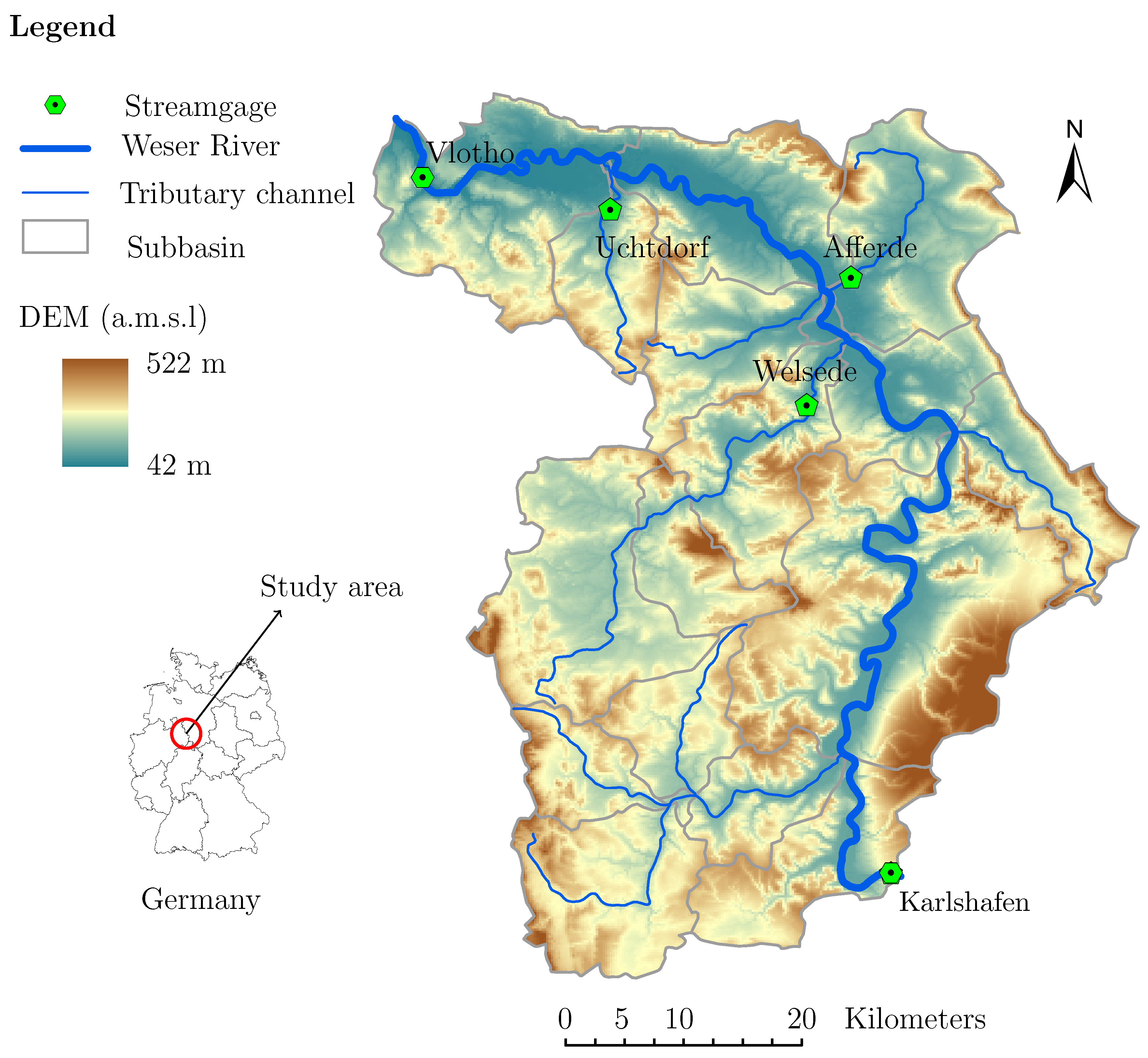
The study area is a segment of the Weser River between Bad Karlshafen and Vlotho located in Lower Saxony and North Rhine-Westphalia, Germany (Figure 1). This Weser River segment has a total length of 142 km, an average slope of 0.01%. Daily inflow data at the Karlshafen gauging station and outflow data at the Vlotho gauging station were obtained from the the Wasser und Schifffahrtsdirektion Mitte. Daily streamflow data at three tributary channels were taken from the Niedersächsische Landesbetrieb für Wasserwirtschaft, Küsten- und Naturschutz (NLWKN). The drainage areas corresponding to the Karlshafen and Vlotho gauging stations are 14,790 km and 17,620 km, respectively. The tributary river Emmer was simulated at the gauging station Welsede (509 km). Weather data in this area were taken from the Deutscher Wetterdienst. The Digital Elevation Model (DEM) of 200 m resolution shows that the elevation of the study area varies between 42 and 522 m above mean sea level (a.m.s.l). Land cover and soil maps were obtained from the CORINE Land Cover project and the Bundesanstalt für Geowissenschaften und Rohstoffe (BGR), respectively.
4.2. Simulation Scenarios
Due to the similarities (1) in the variable storage subroutine between SWAT2000, SWAT2005, and SWAT2009 and (2) in the Muskingum routing subroutine between SWAT2009 and SWAT2012, simulations in this study were only performed with four different routing subroutines (Table 1). The numerical instability due to neglecting the condition in Equation (14) in the Muskingum routing subroutine of SWAT2000 (or SWAT2005) was discussed in detail by Kim and Lee [10]. In order to compare the effects of using different hydrologic routing subroutines (Table 1) on the simulated streamflow, the runoff generated from the intermediate catchments was simulated using the same subroutines and parameters in all scenarios. This is done to ensure that the simulated runoff entering the Weser River in all simulations is the same. In addition, to minimize the error of simulated flow at the outlet of the study area, (1) observed flow at the Uchtdorf, Afferde, and Welsede gauging stations was used as model inflow condition, and (2) contributing flow from other ungauged tributary channels and intermediate subbasins was simulated by using parameters obtained when calibrating for streamflow at the Welsede gauging station. For hydrologic routing, the best calibrated parameter values of the variable storage and Muskingum in this study are as follows: Manning’s roughness coefficient CH_N(2) = 0.025, MSK_X = 0.25, MSK_CO1 = 0.75, and MSK_CO2 = 0.25. The channel width (parameter CHW2) was overestimated by the ArcSWAT pre-processing and was corrected by evaluating aerial images. The model was simulated for the years 1990–2000. However, in order to demonstrate the hydrologic routing for flood events and for low flow, shorter time periods were evaluated.
4.3. Results and Discussions
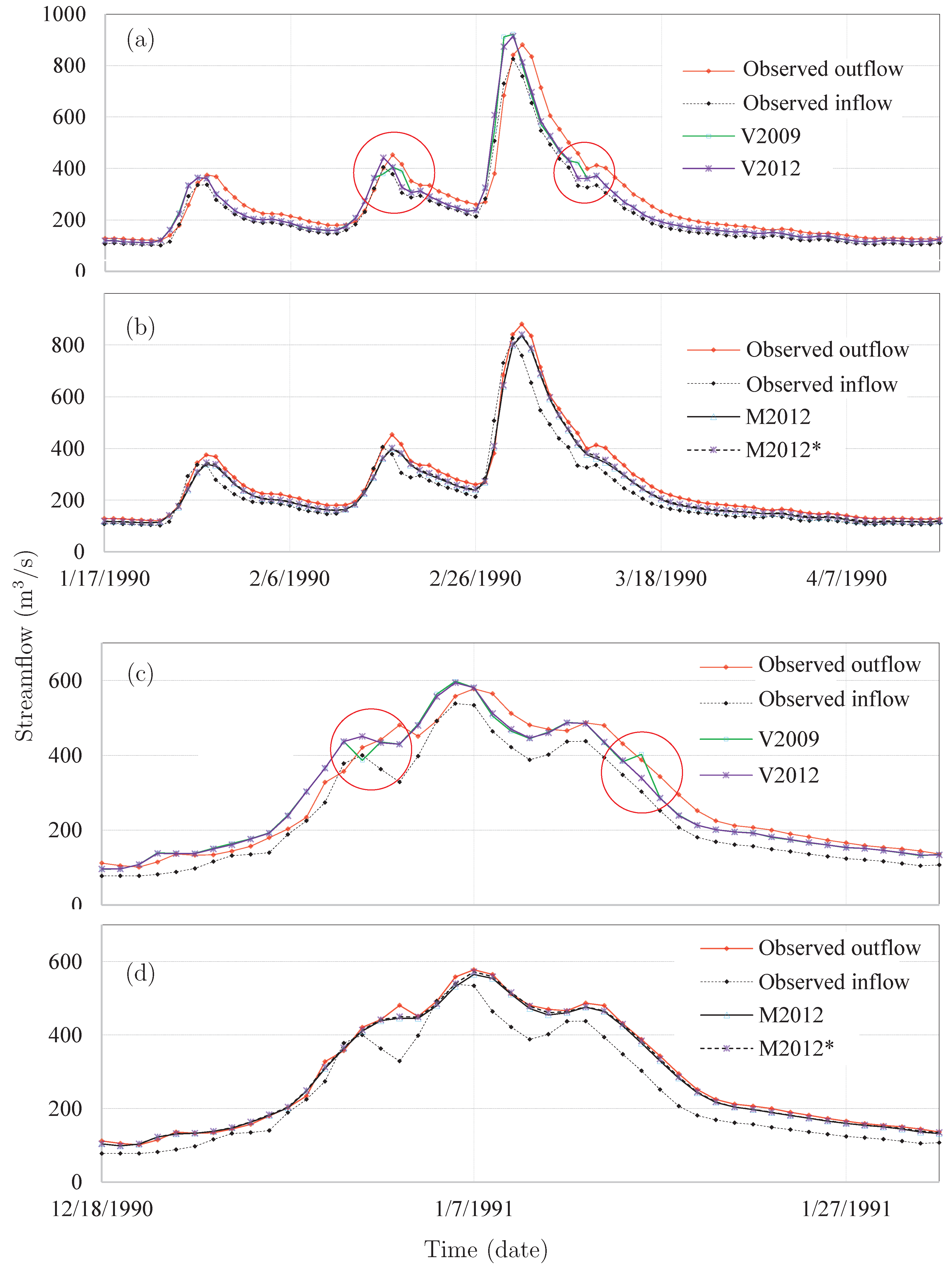
Simulated streamflow at the Vlotho gauging station easily shows by visual evaluation that V2009 and V2012 failed to perform flood routing (Figure 2a,c). Nash–Sutcliffe efficiency (NSE) [17] and percentage bias (PBIAS) show good values due to the high influence of inflow taken from observed values (Table 2). For example, (1) the timing of simulated peaks is earlier than the observed and (2) the simulated peaks are higher than the observed. The simulated outflow from V2009 and V2012 is almost identical to inflow. The variable storage method does not show a transformation of the flood wave as it moves downstream. V2012 simply assigns inflow as outflow as previously discussed. The similarities between simulated outflow from V2009 and V2012 are due to the fact that V2009 assigns C = 1 most of the time (to avoid C > 1). We found that the unphysical oscillation of simulated flow with V2009 (as shown in the red circles in Figure 2a,c) occurs when flow in the channel flood plain occurs (or disappears). This is due to the assumption about the flood plain geometry and the use of the Manning’s equation. The flood plain width in SWAT is assumed five times the top width of the channel. When flow starts to change from non flood-plain flow to flood-plain flow (or from flood-plain flow to non flood-plain flow), there is a sudden increase (or decrease) in the flow velocity, the travel time T, the storage coefficient C, and ultimately the simulated outflow. We also found that, in the case C > 1, changing the simulation time step during a simulation in order to have C ≤ 1 could also cause the same problem. The simulation time step should be the same for the entire simulation time. A solution to this problem could be selecting a sufficiently small time step (small t) and a sufficiently long river section (high T), but this is event-based and reach-specific. Therefore, the V2009 and V2012 are not practical for long-term simulations at basin-scale.
Figure 2b,d shows simulated outflow at the Vlotho gauging station using M2012 and M2012*. It is seen that simulated outflow from M2012 and M2012* is better than that from V2009 and V2012 (Figure 2a,c and Table 2). The timing of simulated peaks and the shape of the flood wave matched well with observed outflow. The effect of the overestimation of channel evaporation with M2012 is negligible in this case (Figure 2b,d) because the flow rate is high compared to the evaporation rate. The underestimation of flow from M2012 and M2012* as shown by the PBIAS (Table 2) is also due to the underestimation of flow from tributary reach and intermediate subbasins. The effect of overestimating channel evaporation with on simulated streamflow with M2012 during flood events is negligible (Figure 2 and Table 2).
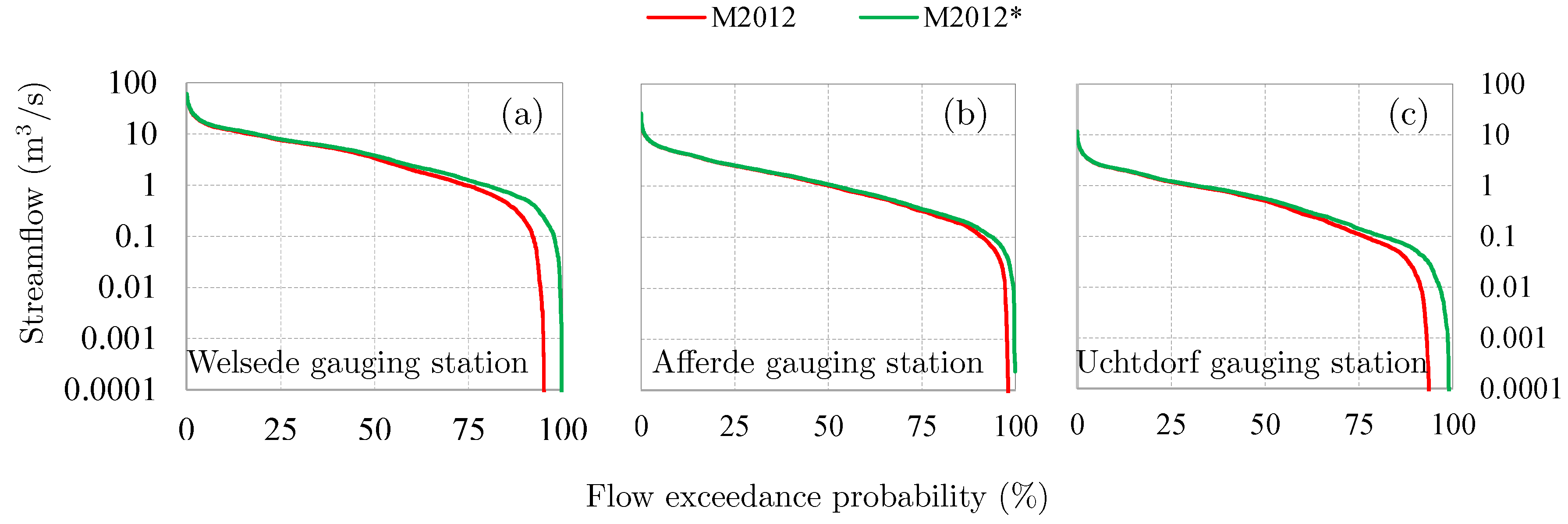
The effect of overestimation of channel evaporation on simulated streamflow with M2012 is more pronounced when the entire catchment response is evaluated, especially during periods of low flows. Figure 3a–c shows the simulated flow duration curves at three gauging stations (Figure 1) using M2012 and M2012* during 1990–2000. It is seen that the effect of overestimating channel evaporation on low flow (<Q75) is significant. The simulated streamflow volumes (from 1990 to 2000) with M2012 at the Welsede, Afferde, and Uchtdorf gauging stations are 6.3%, 2.4%, and 4.2%, respectively, less than that with M2012*. The effect of overestimation of channel evaporation with M2012 is expected to increase with an increase in (1) river density, (2) channel evaporation rate (arid or semi-arid areas), (3) river width/depth ratio, and (4) the number of sub-daily time steps used in the Muskingum routing subroutine.
5. Conclusions and Recommendations
In this study, we validated and corrected the hydrologic routing subroutines of different SWAT revisions. Results show that there are major issues in both routing subroutines of SWAT, the variable storage and Muskingum. In case of simulation with the variable storage method, (1) SWAT2012 (Revision 664) does not perform hydrologic routing, and (2) unphysical oscillation of simulated flow was observed with SWAT2009 due to the assumption of the flood plain geometry and the use of the Manning’s equation. In case of simulation with the Muskingum subroutine (SWAT2009 Revision 528 and SWAT2012 Revision 664), (1) a high portion if not all of streamflow volume in low flow periods could be lost due to overestimation of channel evaporation, (2) unphysical results could be obtained due to violating the numerical stability condition, and (3) channel transmission loss is underestimated if it is activated. A corrected Muskingum subroutine from SWAT2012 (Revision 664), here called M2012*, shows a good estimation of the two flood waves in our simulation period and a reduced channel evaporation loss.
Based on the results of this study, we suggest that the SWAT user community check and upgrade their existing SWAT models, which used the aforementioned affected SWAT versions. It is recommended that whether the updated result supports their methods and conclusions be checked. This is especially important for studies focused on (1) basins with short reaches, and/or (2) low flow simulation, (3) event-based simulation, and/or (4) basins in (semi-) arid regions, where evaporation is high but channel transmission losses can be significant. A bias contribution of streamflow in an order of 5% is considered significant for the calibration of other components of the model, in particular during low flow periods, where soil and groundwater parameters might be estimated wrongly due to the error in channel routing. Although SWAT+ is announced as the next generation of SWAT, there are still many SWAT users working with existing SWAT models. Therefore, verifications of other functions of SWAT are also suggested in order to decrease the model structure uncertainty.
Author Contributions
V.T.N. and J.D. designed the study. V.T.N. carried out the simulation. V.T.N., D.A.T. and B.U. reviewed the SWAT codes. All authors wrote the draft and contributed to the final version of the manuscript.
Funding
This research received no external funding. The APC was funded by the Open Access fund of Leibniz Universität Hannover.
Acknowledgments
The authors thank three anonymous reviewers for their constructive comments which improved the quality of the manuscript.
Conflicts of Interest
The authors declare no conflict of interest.
References
- Chow, V.T. Handbook of Applied Hydrology; McGraw-Hill: New York, NY, USA, 1964. [Google Scholar]
- Arnold, J.G.; Srinivasan, R.; Muttiah, R.S.; Williams, J.R. Large area hydrologic modeling and assessment Part I: Model development. Trans. ASABE 1998, 34, 73–89. [Google Scholar] [CrossRef]
- Neitsch, S.L.; Arnold, J.G.; Kiniry, J.R.; Williams, J.R. Soil and Water Assessment Tool Theoretical Documentation Version 2009; TexasWater Resources Institute, Texas A&M University: College Station, TX, USA, 2011. [Google Scholar]
- Krysanova, V.; Arnold, J.G. Advances in ecohydrological modelling with SWAT—A review. Hydrolog. Sci. J. 2008, 53, 939–947. [Google Scholar] [CrossRef]
- Arnold, J.G.; Fohrer, N. SWAT2000: Current capabilities and research opportunities in applied watershed modelling. Hydrol. Process. 2005, 19, 563–572. [Google Scholar] [CrossRef]
- Gassman, P.; Reyes, M.; Green, C.; Arnold, J. The soil and water assessment tool: Historical development, applications, and future research directions. Trans. Am. Soc. Agric. Biol. Eng. 2007, 50, 1211–1250. [Google Scholar] [CrossRef]
- Williams, J.R. Flood routing with variable travel time or variable storage coefficients. Trans. ASABE 1969, 12, 0100–0103. [Google Scholar] [CrossRef]
- Cunge, J.A. On the subject of a flood propagation computation method (Muskingum method). J. Hydraul. Res. 1969, 7, 205–230. [Google Scholar] [CrossRef]
- United States Department of Agriculture—Natural Resources Conservation Service. National Engineering Handbook: Part 630—Hydrology; USDA Soil Conservation Service: Washington, DC, USA, 2004.
- Kim, N.W.; Lee, J. Enhancement of the channel routing module in SWAT. Hydrol. Process. 2010, 24, 96–107. [Google Scholar] [CrossRef]
- Pati, A.; Sen, S.; Perumal, M. Modified channel-routing scheme for SWAT model. J. Hydrol. Eng. 2018, 23, 04018019. [Google Scholar] [CrossRef]
- Diskin, M.H. On the solution of the Muskingum flood routing equation. J. Hydrol. 1967, 5, 286–289. [Google Scholar] [CrossRef]
- Arnold, J.G.; Williams, J.R.; Maidment, D.R. Continuous-time water and sediment-routing model for large basins. J. Hydraul. Eng. 1995, 121, 171–183. [Google Scholar] [CrossRef]
- Neitsch, S.L.; Arnold, J.G.; Kiniry, J.R.; Williams, J.R. Soil and Water Assessment Tool Theoretical Documentation Version 2005; TexasWater Resources Institute, Texas A&M University: College Station, TX, USA, 2005. [Google Scholar]
- Arnold, J.G.; Kiniry, J.R.; Srinivasan, R.; Williams, J.R.; Haney, E.B.; Neitsch, S.L. Soil and Water Assessment Tool Input/Output Documentation 2012; Texas Water Resources Institute Technical Report No. 439; Texas A&M University System: College Station, TX, USA, 2012. [Google Scholar]
- Neitsch, S.L.; Arnold, J.G.; Kiniry, J.R.; Williams, J.R.; King, K.W. Soil and Water Assessment Tool, Theoretical Documentation, Version 2000; TexasWater Resources Institute, Texas A&M University: College Station, TX, USA, 2002. [Google Scholar]
- Nash, J.E.; Sutcliffe, J.V. River flow forecasting through conceptual models. Part 1: A discussion of principles. J. Hydrol. 1970, 10, 282–290. [Google Scholar] [CrossRef]
Figure 1.
Location of the Weser River segment and its tributary rivers.

Figure 2.
Simulated outflow at the Vlotho gauging station for two flood events using (a,c) V2009 and V2012 and (b,d) M2012 and M2012*.
Figure 2.
Simulated outflow at the Vlotho gauging station for two flood events using (a,c) V2009 and V2012 and (b,d) M2012 and M2012*.

Figure 3.
Flow duration curves of the simulated streamflow (logarithmic scale) at the (a) Welsede, (b) Afferde, and (c) Uchtdorf gauging stations during 1990–2000 with M2012 and M2012*.
Figure 3.
Flow duration curves of the simulated streamflow (logarithmic scale) at the (a) Welsede, (b) Afferde, and (c) Uchtdorf gauging stations during 1990–2000 with M2012 and M2012*.


Table 1.
List of the hydrologic routing subroutines used for this study.
| Flood Routing Subroutine | Description |
|---|---|
| V2012 | Variable Storage routing subroutine of SWAT2012 |
| V2009 | Variable Storage routing subroutine of SWAT2009 |
| M2012 | Muskingum routing subroutine of SWAT2012 |
| M2012* | corrected Muskingum routing subroutine of SWAT2012 |
Table 2.
Model performance statistics for flood event 1 (17 January 1990 to 17 April 1990, Figure 2a,b) and flood event 2 (18 December 1990 to 1 February 1991, Figure 2c,d).
| Subroutine | Flood Event 1 | Flood Event 2 | ||
|---|---|---|---|---|
| NSE | PBIAS | NSE | PBIAS | |
| V2012 | 0.898 | 7.24 | 0.955 | 1.34 |
| V2009 | 0.902 | 7.24 | 0.953 | 1.27 |
| M2012 | 0.975 | 8.49 | 0.995 | 2.35 |
| M2012* | 0.981 | 7.25 | 0.997 | 1.49 |
© 2018 by the authors. Licensee MDPI, Basel, Switzerland. This article is an open access article distributed under the terms and conditions of the Creative Commons Attribution (CC BY) license (http://creativecommons.org/licenses/by/4.0/).
Share and Cite
MDPI and ACS Style
Nguyen, V.T.; Dietrich, J.; Uniyal, B.; Tran, D.A. Verification and Correction of the Hydrologic Routing in the Soil and Water Assessment Tool. Water 2018, 10, 1419. https://doi.org/10.3390/w10101419
AMA Style
Nguyen VT, Dietrich J, Uniyal B, Tran DA. Verification and Correction of the Hydrologic Routing in the Soil and Water Assessment Tool. Water. 2018; 10(10):1419. https://doi.org/10.3390/w10101419
Chicago/Turabian StyleNguyen, Van Tam, Jörg Dietrich, Bhumika Uniyal, and Dang An Tran. 2018. "Verification and Correction of the Hydrologic Routing in the Soil and Water Assessment Tool" Water 10, no. 10: 1419. https://doi.org/10.3390/w10101419
Note that from the first issue of 2016, this journal uses article numbers instead of page numbers. See further details here.