Numerical and Physical Investigation of the Performance of Turbulence Modeling Schemes around a Scour Hole Downstream of a Fixed Bed Protection

Department of Civil and Environmental Engineering, Incheon National University, 119 Academy-ro, Yeonsu-gu, Incheon 22012, Korea
*
Author to whom correspondence should be addressed.
Water 2018, 10(2), 103; https://doi.org/10.3390/w10020103
Submission received: 17 November 2017
/
Revised: 19 January 2018
/
Accepted: 22 January 2018
/
Published: 26 January 2018
Abstract
:Local scour occurs around hydraulic structures such as piers, bed protections, and dikes. In this study, the turbulent flow around a scour hole downstream of a fixed bed protection was investigated. Numerical modeling with OpenFOAM was applied to compute the flow velocity and turbulent kinetic energy with respect to flow conditions by changing water depth. A proper computational grid size and time step for simulations are suggested. Three typical turbulent models, , , and , were considered for simulating the flow around a scour hole. The performances of the three models were evaluated by comparing them with numerical and laboratory experimental results. Mean flow velocity profiles computed by the three turbulent schemes are generally in good agreement with laboratory measurements. However, has a limitation in simulating reversal flow in the scour hole, and the model does not predict turbulent kinetic energy well near the bottom. Thus, this study found that the most suitable turbulent model for simulating flow around a scour hole downstream of a fixed bed protection is the model.
1. Introduction
Local scour occurs around hydraulic structures such as bridge piers, abutments, or bed protections and is considered as one of the most common causes of hydraulic structure failures [1,2]. It leads to unsafe conditions that require significant maintenance efforts at those positions. Therefore, studying scour development and its flow properties is of great importance to riverbed protection and has received attention from both academic researchers and engineers.
Normally, physical experiments are carried out to investigate a scour structure [3,4]. However, this method is both time- and cost-intensive, especially for large-scale experiments, for studying the involved parameters [5]. Therefore, numerical modeling has recently been widely applied because of its advantages in minimizing scaling effects and facilities [6,7]. This popular method also benefits from accurate results from advanced capabilities of modern computers. However, the flows in nature are commonly under high Reynolds numbers and fully turbulent conditions that still cause difficulties for modeling. In particular, accurate calculations of the flow separation in the scour region require significant effort.
In most numerical models, Navier–Stokes equations are solved to capture the dynamics of the fluid, and the direct numerical simulation (DNS) is considered the most accurate [8] for modeling the turbulence characteristics of the flows. However, this method is very computationally demanding because it resolves the smallest scales of flow that is presented, and difficult to simulate for large applications. Therefore, the Reynolds-averaged Navier–Stokes (RANS) formulation is typically chosen because it solves mean velocity profiles and effects of the temporal velocity fluctuation. This is because of its capacity of decomposing the velocity into mean and the fluctuation components. This approach helps to save computational cost by not resolving the smallest turbulent scales.
The RANS approach in numerical calculations, such as OpenFOAM (The OpenFOAM Foundation Ltd., London, United Kingdom) Toolbox, supports various schemes to investigate the turbulence, and the most common models are , , and [9,10]. However, these schemes were developed based on particular techniques, suitable for each special case. They need to be investigated before applying the models to have accurate results. Therefore, the objective of this study is to evaluate the performance of those RANS turbulence models for fully developed incompressible turbulent flows around scour holes in an open channel. Because it is very difficult to simulate turbulent flows in an open channel with a scour hole as the reverse flow occurs in the scoured region, numerical schemes and initial and boundary conditions need to be properly set.
The present study was conducted for an incompressible steady stage open channel flow with a scour hole developing on a movable sand bed channel downstream of a fixed bed; moreover, this setting is characteristic of hydraulic structures such as bed protection. It should be noted that the roughness of the bed changes significantly upstream and downstream of the bed protection. Concrete bed protection is commonly constructed on an alluvial stream and the scour occurs on the initial erodible bed downstream of the protection. For the upstream part, concrete protection is much smoother than for the downstream part, where the initial bed comes in contact with sediments. The abrupt change in the roughness of the bed makes the flow more complicated; therefore, proper numerical methods should be applied to simulate the turbulent characteristics.
The bed profile and other flow conditions were imported from our physical experiment [11]. Various turbulence schemes were applied to compare the accuracy of the selected mathematical models’ capability of simulating the turbulent flow. The numerical results of flow streamline, velocity distribution, and turbulent kinetic energy profile were compared to the experimental data to suggest the best method of numerical estimations.
2. Methodology
2.1. Laboratory Experiment
To investigate the hydraulic characteristics of a scour hole developed in a sand bed channel, we conducted a laboratory experiment with the setting as plotted in Figure 1. The physical study included a 12.5 m long and 0.6 m wide channel that runs water between two parallel vertical glass walls. Water was pumped into the channel with a maintained volumetric flow rate (Q) of 0.035 m3/s, and the water depth was adjusted by controlling a tail gate at the end of the channel. Two experimental cases were studied, and the conditions are as shown in Table 1.
In this table, h is the water height (m), d50 is the mean particle size by weight (mm), and u is the inlet velocity of the flow (m/s), which is calculated by
where A (m2) is the area of the inlet boundary.
The Reynolds number is calculated by
where is the kinematic viscosity of water (m2/s); the reference length D (m) for this calculation is the water height at the inlet (h).
The channel bed was divided into two parts: the upstream one was a 4.5 m long fixed bed made of acrylic to produce a smooth condition; the downstream one was an 8 m long movable bed filled up with very coarse sand, and the mean particle size by weight (d50) was set to 1.2 mm to ensure the development of scour. The bed roughness was zero at the upstream part while the roughness at the downstream part was set to be equivalent to the median size of 1.2 mm. This laboratory experiment was carried out until a stable stage, at which there was no further increase in the scour hole was reached. The experiments took up to 12 days to perform. At the equilibrium stage, we used an acoustic Doppler velocimeter (ADV) system to measure the bed and velocity profiles.
In the ADV system, the measurement of three-dimensional flow velocity and bed elevation was conducted with a down-looking Vectrino (Nortek AS, Vangkroken, Norway). The vertical alignment of the sensor was controlled by an auto-traverse system mounted on a moving carriage and carried manually. The two-axis auto-traverse system can be controlled with a digital panel, which is connected to a personal computer. Additionally, the auto-traverse has the riveting plate for the positioning measuring apparatus. This system can capture the data at points 2 mm above the channel bottom. All data were measured for over 30 s, generally longer in the scour hole, at 50 Hz. The time-averaged flow velocities and turbulence properties in three dimensions were calculated with an ensemble averaging method using an integral time scale and autocorrelation function in time.
2.2. Numerical Investigation
This study focused on numerical modeling methods of estimating turbulent characteristics around a scour hole. We applied three different turbulence schemes, , , and , to determine the most appropriate one for simulating the complex flows around the scour. Our methods from both the physical and numerical models will help engineers to select an appropriate or suitable numerical turbulent modeling scheme around the hole.
2.2.1. Governing Equations
The open computational fluid dynamics library, OpenFOAM, was employed to perform the numerical modeling task. OpenFOAM is open-source software utilizing a finite volume method to solve the governing equations. As mentioned, the model is based on the Reynolds-averaged Navier–Stokes equation and solves the governing equations in the ensemble-averaged form. The equations for incompressible flow have been previously discussed in many studies such as [7,12,13].
The continuity equation is given by
and its Reynolds-average Navier–Stokes equation is
where u, U, and are the instantaneous velocity, mean velocity, and fluctuating velocity, respectively; t represents time; and P denote density and pressure, respectively; is the molecular viscosity; is the mean strain-rate tensor.
2.2.2. Turbulence Modeling
In OpenFOAM library, the RANS turbulence models are based on the concept of the eddy viscosity () introduced by Boussinesq in 1887 [14]. This method relates the Reynolds stress to the mean properties of the flow by using the eddy viscosity.
The RANS standard k-ε model is the simplest and one of the most common turbulence models. It is a two-equation model that includes two extra transport equations to represent the turbulent properties of the flow: the turbulent kinetic energy (k) and the turbulent energy dissipation (). The former and the latter variables determine the energy and the scale of the turbulence, respectively. The transport equations for these two variables were first introduced in [15] and are presented as
where Gk and Gb are, respectively, the generation of turbulent kinetic energy due to the mean velocity gradient and buoyancy; Sk and are the moduli of the mean rate-of-strain tensors of k and , respectively. Finally, and are the diffusion rates for k and , respectively, and are derived from the turbulent mixing length [16].
Additionally, the dynamic turbulent viscosity in this model is defined as
where , , , and are experimental constants proposed as in Table 2, which are only applicable to high-Reynolds-number flows [17].
Because the standard model is a high-Reynolds-number model, it has a limitation in solving flows close to the wall where the Reynolds number is low because of the small velocity profiles in this region. In the model, the closest mesh point to the wall is located at the turbulent boundary layer, and modeling of the viscous sublayer and buffer layer is avoided. Therefore, in this study, the wall function was applied to enhance the computing accuracy near the wall. This function is required to model the influence of the grain roughness to the flow. Additionally, to ensure consistency in the research, we enabled this wall function for both the and case studies.
The RANS model is also a two-equation model developed by Wilcox in 1993 [18] that uses a similar approach and has the same definition of k in the model. However, instead of using turbulent energy dissipation ε, this model uses the rate of dissipation of energy per unit volume and time, the so-called specific dissipation rate ω. In contrast to the model, the model can be used in the regions close to the wall where turbulence is very low and k tends to be zero [12].
In this model, the turbulent viscosity is computed by
The modeled transport equations for k and ω in this model are
Here, is the generation of specific dissipation rate due to the mean velocity gradient, and is the modulus of the mean rate-of-strain tensors of ω. The constants were chosen as [19].
The RANS (shear–stress transport) model is a two-equation turbulence model developed by Menter in 1994 [20] based on the previous two models. Basically, the model is similar to the standard model although the former includes several improvements and other constant variables. This method effectively blends the accurate formulation of the model in the near-wall region with the free-stream independence of the model in the far-field region, away from the wall. This blending function allows switching the turbulence schemes between near-wall and far-field regions, thus reducing the computational requirement [9,10].
The transport equation for turbulent kinetic energy k in this model is the same as that for the basic model mentioned before, while the equation for ω can be written as
In this equation, represents the cross-diffusion term, which is an addition to the standard model.
2.2.3. Numerical Setup
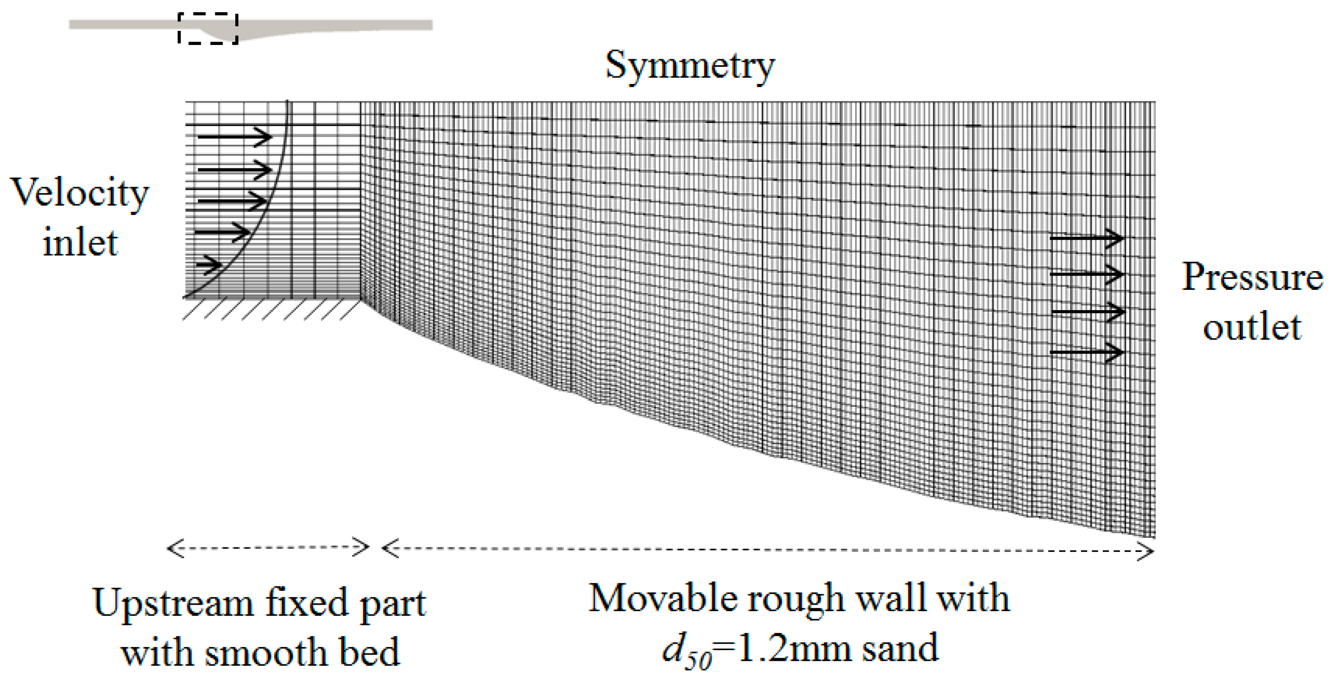
The domain scale of the numerical modeling was the same as the physical experiments in two dimensions. The physical one was conducted in a 0.6 m wide channel, while the numerical one was considered as a two-dimensional flow, in both horizontal and vertical directions, because the physical model was symmetrical along the centerline of the channel. The bed profiles were imported from the physical experimental results at the equilibrium stage. Because the boundary conditions and computation mesh are important for the numerical modeling, and have a strong impact on the output, they should be selected properly, as presented in Figure 2. The flow was set up as velocity inlet and pressure outlet at the upstream and downstream boundaries, respectively. The upper boundary, which is the atmosphere in the physical experiment, was set as a symmetry condition. The bottom of the channel was divided into two parts, a smooth wall and a rough wall with respect to the acrylic and sand beds in the physical experiment. The “wall” boundary condition allowed the application of the wall function and a specified roughness as well. The value for roughness was set to zero for the smooth wall, and an equivalent value of d50 = 1.2 mm sand particle for the rough wall.
The mesh was gradually refined toward the bottom to enhance the accuracy near the walls, as shown in Figure 2. The grid size in the scour region was also meshed smaller than other areas to have better results where the flow is complicated. Errors from the discretization were avoided by selecting an optimal combination of grid and time step. A grid size and time step convergence study was conducted for selecting the appropriate parameters. In this study, the basic model was used. Three grid sizes (accounting for the cell closest to the wall) of 1 mm, 1.5 mm, and 3 mm and three time steps of s, s, and s were compared, as shown in Figure 3. The horizontal velocities ux were recorded 4.5 m downstream.
Comparison indicates that a square grid of minimum Δz = 1.5 mm (near the wall) and maximum 10 mm (close to the atmosphere) and a time step of Δt = s are small enough to obtain results within 0.1% of the higher resolution cases. Simulations ran for 120 s, which proved to be enough for the simulated results to reach the stabilized state. The initial condition values for the model parameters were calculated and set as presented in Table 3.
3. Results and Discussion
The numerical results of the streamline, flow axial velocity, and turbulence kinetic energy were compared to the laboratory experimental measurements to investigate the performance of the three turbulent modeling schemes in a scour hole.
3.1. Streamline
Both cases of the physical experimental results show flow separation in the scour hole as shown in Figure 4. This phenomenon is of significant importance in moving or transporting the sediment particles from the bed. It also helps the development of the scour hole. As can be seen here, a backflow exists close to the bed in a region called the deceleration zone [21]. Referring to Figure 4, the size of flow circulation x/h, a dimensionless number of real distance x divided by initial water height h, reaches to x/h = 6.86 for Case Exp1 (slower flow) and x/h = 6.67 for Case Exp2 (faster flow).
Among the three turbulence schemes, the model seems to be the closest to the experimental data for both Exp1 and Exp2. This model produces circulation flow right downstream of the transition point (at x/h = 0), where the roughness of the bed changes abruptly. This result shows good agreement with the experimental data. The axial lengths of the flow circulation in this model are approximately at x/h = 6.79 and 6.25 for Cases SST1 and SST2, respectively, and fit quite well with Exp1 and Exp2.
The standard model, as can be seen in Figure 4, fails in predicting the occurrence of this flow separation. The result from does not show the circulation except for the smooth straight streamlines near the transition point. However, the standard successfully shows the presence of backflow in the scour hole. This result is not surprising because the model is more suitable for modeling the high-turbulence flows in this area than the model. However, the model over-predicts the size of the circulation. The maximum horizontal lengths of separation flows in Cases kε1 and kε2 are located x/h = 9.38 and 7.95 downstream, which are, respectively, 1.2 and 1.4 times greater than the experimental results.
3.2. Velocity Profile
Along with the results of the streamline, which show the flow motion, the velocity profile is also an important result for analyzing the flow characteristics. The streamline plots are normally not accurate enough to distinguish the flow separation zone [22], and a velocity profile is usually needed to obtain the exact ending position of the backward velocity vectors. The numerical and experimental longitudinal velocities ux of the flow along the channel are shown together in Figure 5.
The velocity profile of the model clearly shows the absence of backward velocity vectors or minus velocity values as plotted for both flow conditions (see Figure 5). This result explains why the model does not predict a circular form in the scour region, as can be seen in Figure 4. The model can perform well for velocity profiles before the transition point as well as at the far downstream part after x/h = 10.4 in Case 1 or x/h = 8.3 in Case 2, as shown in Figure 4. However, the profile right at x/h = 0 shows a slight difference close to the wall. While other models produce a logarithmic curve in the velocity at the intersection between near-wall and far-wall regions, the model is not accurate because it has a much stronger bed strain there. This may be due to the sudden change of bed roughness at this point, therefore the model seems to have a limitation in simulating flows around an abrupt roughness change. This can be seen in Figure 6, which shows the wall shear stress results of the three turbulence schemes. As can be seen from the figure, after the transition point (x = 0 m), where the bed roughness increases abruptly, both the and models gave reasonable results of increasing wall shear stress. However, the model shows a decrease in this parameter. This small shear stress could not produce the circulation flow in the scour hole of this simulation. Moreover, the model gives significantly inaccurate results for both the magnitude of the values as well as the trend of the velocity profile in the scour hole. In this study, the model over-predicts the flow velocity inside the scour hole and under-predicts it in the upper water layer, with a maximum root mean square error (RMSE) reaching up to 0.137, as shown in Table 4.
Here, the RMSE is calculated by:
where unume. is the velocity results from numerical modeling, and uexp. is the integrated velocity data from experiments, which is used as the reference signal.
The standard model is slightly better than the model; however, the data for the former are no better than the latter in comparison with experimental data. The performance of the standard model is also very good upstream of the transition point, though it needs to flow further downstream than the model for it to obtain results similar to those obtained using the experimental data (x/h = 13.9 and 11.7 for Cases kε1 and kε2, respectively). For the upstream parts of these x/h distances, the turbulence model over-predicts the backflow, which is represented as a negative velocity, near the wall and under-predicts inside the scour hole. The overall mean error, compared to the experimental data, lies between 0.043 and 0.056.
The velocity profiles from the model are the best in both study cases. However, some deviation can still be found at some points such as at z > 0 at x/h = 7.1 or 10.4 for Case SST1. Additionally, in the scour regions of x/h = 2.1 for Case SST1 or x/h = 1.7 for Case SST2, this model seems to under-predict the flow velocity, with an RMSE approximately between 4 and 5%. Furthermore, the overall mean difference of the numerical result, compared to the experimental data of the model, is between 0.0407 and 0.0413, while the overall mean difference of the numerical result for the and models is between 0.0431 and 0.0561 and between 0.0448 and 0.0560, respectively (see Table 4).
3.3. Turbulent Kinetic Energy
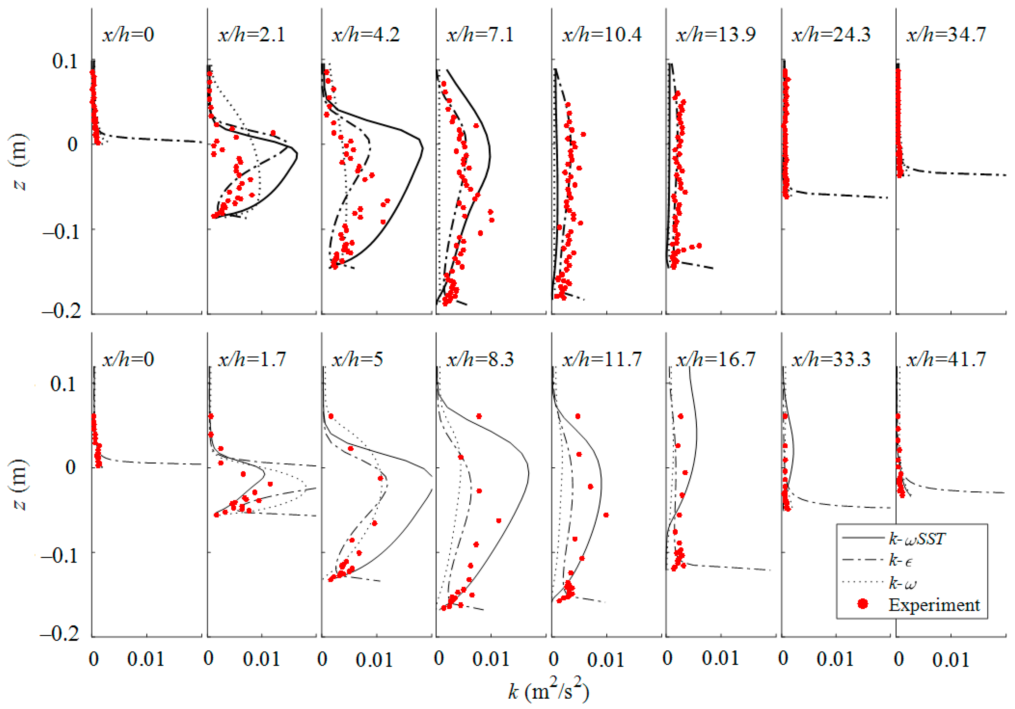
A flow running through a rough bed, especially with sudden roughness changes as in our study, induces turbulence, which results in resistance to the flow. The turbulent kinetic energy (k), defined by the mean kinetic energy associated with these turbulences in the flow, can be used to analyze the turbulence property of the flow. Normally, the cross-sectional plots of k are useful for showing the location and intensity of flow turbulence. The experimental and numerical results are shown together in Figure 7.
The turbulent kinetic energy plots show the existence of a relatively high-turbulence region located right downstream of the flow separation zone for both flow conditions. The value of k increases dramatically in the scour holes compared to other regions. As flow goes downstream from this part, the turbulence energy decreases and eventually reaches a constant value, which is similar to the turbulent kinetic energy upstream of the transition point.
However, the standard model shows the least accurate results in calculating k near the wall. The turbulent kinetic energy is almost zero close to the wall for the and models, while it is extremely high for the model. This result of k clearly shows the weakness of the model; i.e., it is not suitable for modeling flows near the wall. Theoretically, the turbulence model is a high-Reynolds-number model that is only able to solve the turbulent region of the flow. The cell adjacent to the wall is placed in the turbulent region; therefore, the modeling of the viscous sublayer and buffer layer should be avoided. As mentioned before, to overcome this, “wall functions” are required to model the influence of the grain roughness to the flow. Furthermore, the application of a wall function in this study does not seem to suffice to help the model to obtain the desired accurate result.
However, the results of the turbulent kinetic energy from the and models also do not fit accurately with the experimental data, even though they are designed to solve the flow under a low Reynolds number and a combined low and high Reynolds number, respectively. Overall, the model underestimates k by an RMSE value between 0.0037 and 0.004, while the model overestimates k by an RMSE value between 0.0031 and 0.0045. Moreover, the data of the model on the scour hole for Case 1 fail in magnitude; in addition, they cannot provide reasonable k profiles. However, both and achieve a better k near the wall than the model.
4. Summary and Conclusions
This study focused on numerical schemes appropriate for modeling the characteristics of a scour hole formed downstream of a fixed bed protection. Three typical two-dimensional turbulence models, , , and , were used in OpenFOAM Toolbox, and the calculated results of velocity and turbulent kinetic energy profiles of the scour hole were compared to a laboratory experimental data set.
The standard and models are recommended for analyzing the velocity characteristics of scour holes because both models simulate reversal flow, which is a distinguishing characteristic of scour holes. The model does not simulate reversal flow. Flow velocity and streamline profiles computed by and models are generally in a good agreement with laboratory data. However, the development of scour holes depends on the turbulent flow near the bottom, at the interface between sediment and water. Therefore, since turbulent characteristics near the bottom of the scour hole need to be simulated as accurately as possible, this study concluded that the model is the most suitable tool for engineering purposes.
Acknowledgments
This work was supported by Post-Doctor Research Program (2017) through Incheon National University.
Author Contributions
Thi Hoang Thao Nguyen performed the numerical modeling, analyzed the data, and wrote the draft version of this manuscript; Jungkyu Ahn revised and edited the manuscript; Sung Won Park designed and conducted the physical experiments.
Conflicts of Interest
The authors declare no conflict of interest.
References
- Shirole, A.; Holt, R. Planning for a comprehensive bridge safety assurance program. Transp. Res. Rec. 1991, 1290, 39–50. [Google Scholar]
- Guney, M.; Aksoy, A.; Bombar, G. Experimental study of local scour versus time around circular bridge pier. In Proceedings of the 6th International Advanced Technologies Symposium, Elazığ, Turkey, 16–18 May 2011. [Google Scholar]
- Dargahi, B. Controlling mechanism of local scouring. J. Hydraul. Eng. 1990, 116, 1197–1214. [Google Scholar] [CrossRef]
- Roy, D.; Matin, M.A. An assessment of local scour at floodplain and main channel of compound channel section. J. Civ. Eng. 2010, 38, 39–52. [Google Scholar]
- Ahn, J.; Yang, C.T. Determination of recovery factor for simulation of non-equilibrium sedimentation in reservoir. Int. J. Sediment Res. 2015, 30, 68–73. [Google Scholar] [CrossRef]
- Nagata, N.; Hosoda, T.; Nakato, T.; Muramoto, Y. Three-dimensional numerical model for flow and bed deformation around river hydraulic structures. J. Hydraul. Eng. 2005, 131, 1074–1087. [Google Scholar] [CrossRef]
- Liu, X.; Garcia, M.H. Three-dimensional numerical model with free water surface and mesh deformation for local sediment scour. J. Waterw. Port Coast. Ocean Eng. 2008, 134, 203–217. [Google Scholar] [CrossRef]
- Konečný, P.; Ševčík, R. Comparison of turbulence models in OpenFOAM for 3D simulation of gas flow in solid propellant rocket engine. Adv. Mil. Technol. 2016, 11, 239–251. [Google Scholar] [CrossRef]
- Ali, A.; Sharma, R.K.; Ganesan, P.; Akib, S. Turbulence model sensitivity and scour gap effect of unsteady flow around pipe: A CFD study. Sci. World J. 2014, 2014, 412136. [Google Scholar] [CrossRef] [PubMed]
- Stahlmann, A. Numerical and experimental modelling of scour at foundation structures for offshore wind turbines. J. Ocean Wind Energy 2014, 1, 82–89. [Google Scholar]
- Park, S.W. Experimental Study of Local Scouring at the Downstream of River Bed Protection. Ph.D. Thesis, Seoul National University, Seoul, Korea, 2016. [Google Scholar]
- Scholz, S. Study on Porous-Medium Wall Functions for k − ε and k − ω Turbulence Models. Bachelor’s Thesis, Stuttgart University, Stuttgart, Germany, 2014. [Google Scholar]
- Ota, K.; Sato, T.; Nakagawa, H. 3D Numerical model of sediment transport considering transition from bed-load motion to suspension—Application to a scour upstream of a cross-river structure. J. JSCE 2016, 4, 173–180. [Google Scholar] [CrossRef]
- Boussinesq, J.V. Cours d’Analyse Infinitésimale en vue des Applications Mécaniques et Physiques; Gauthier-Villars: Paris, France, 1887. [Google Scholar]
- Jones, W.P.; Launder, B.E. The prediction of laminarization with a two equation model of turbulence. Int. J. Heat Mass Transf. 1972, 15, 301–314. [Google Scholar] [CrossRef]
- Prandtl, L. Bericht über Untersuchungen zur ausgebildeten Turbulenz. J. Appl. Math. Mech. 1925, 5, 136–139. [Google Scholar]
- Launder, B.E.; Spalding, D.B. The numerical computation of turbulent flows. Comput. Methods Appl. Mech. Eng. 1974, 3, 269–289. [Google Scholar] [CrossRef]
- Wilcox, D.C. Turbulence Modelling for CFD, 1st ed.; DCW Industries, Inc.: La Canada, CA, USA, 1993. [Google Scholar]
- Wilcox, D.C. Re-assessment of the scale-determining equation for advanced turbulence models. AIAA J. 1988, 26, 1299–1310. [Google Scholar] [CrossRef]
- Menter, F.R. Two-equation eddy-viscosity turbulence models for engineering applications. AIAA J. 1994, 32, 1598–1605. [Google Scholar] [CrossRef]
- Hoffmans, G.J.C.M.; Booij, R. Two-dimensional mathematical modelling of local-scour holes. J. Hydraul. Res. 1993, 31, 615–634. [Google Scholar] [CrossRef]
- Jellesma, M. Form Drag of Subaqueous Dune Configurations. Master’s Thesis, University of Twente, Enschede, The Netherlands, 2013. [Google Scholar]
Figure 1.
Laboratory experiment setup sketch (left) and real picture (right) [11].
Figure 1.
Laboratory experiment setup sketch (left) and real picture (right) [11].
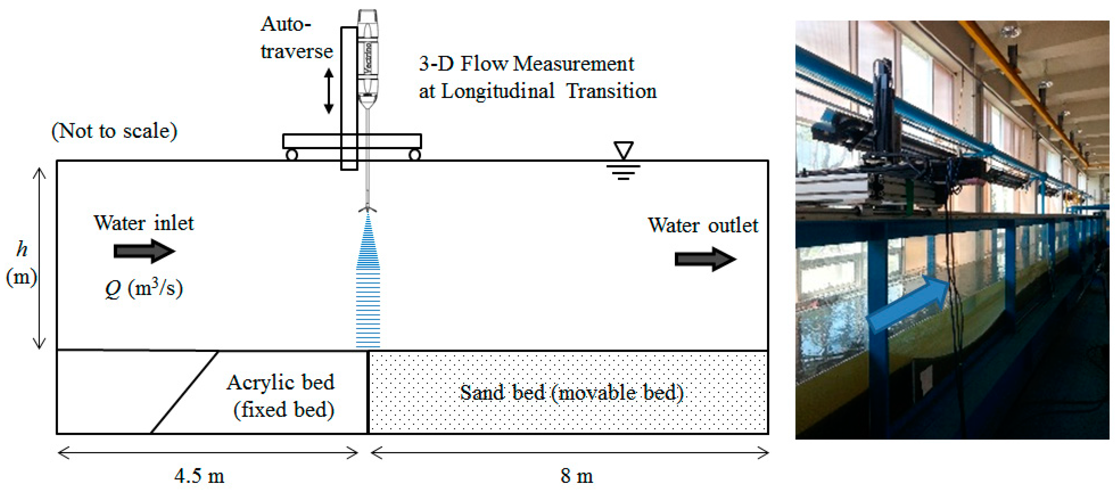
Figure 2.
Schematic model setup and mesh grid (not to scale).

Figure 3.
Grid size and time step convergence.
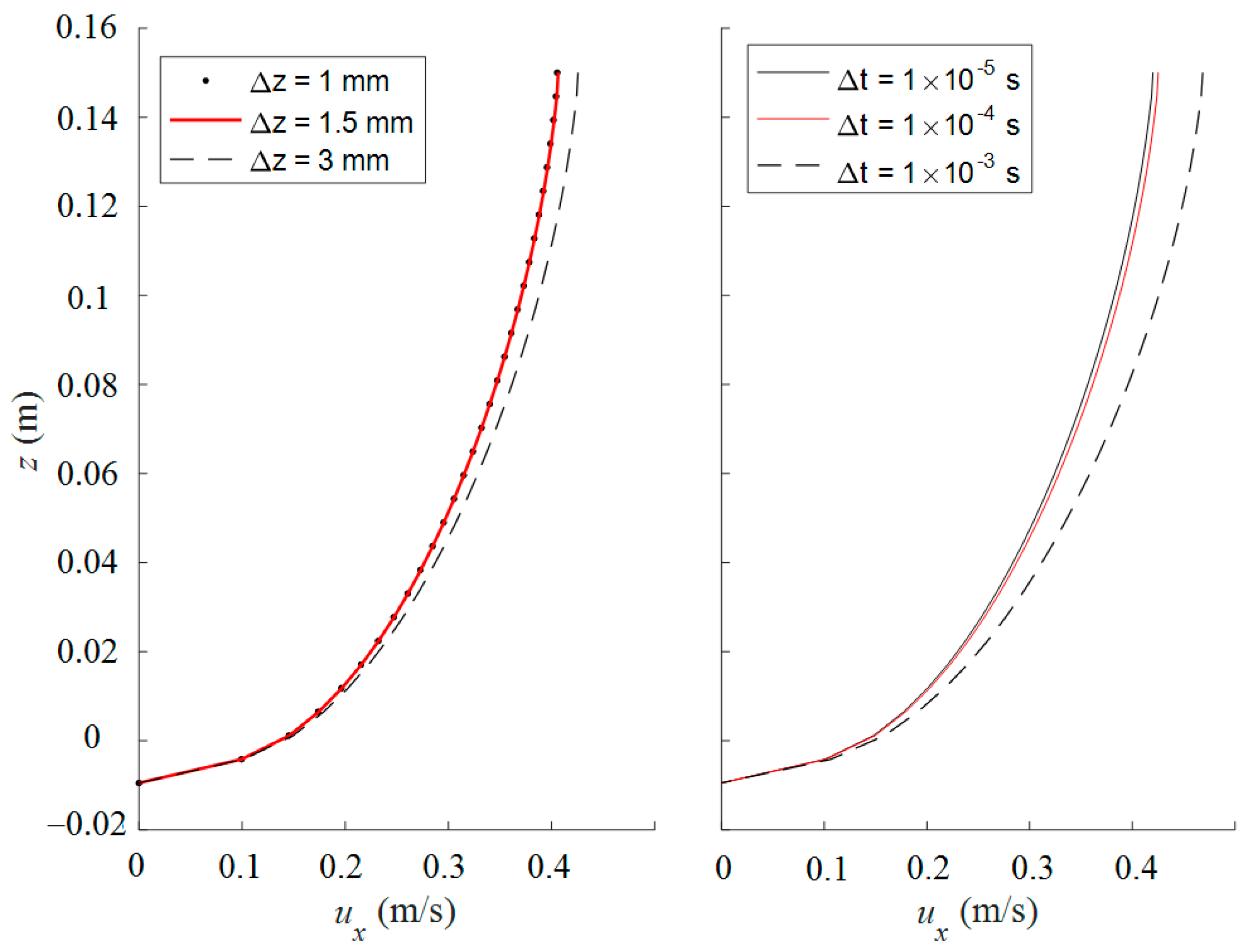
Figure 4.
Numerical flow streamline of different turbulence models along with the experimental data for Case Exp1 (left) and Case Exp2 (right). The red lines represent the channel bed.
Figure 4.
Numerical flow streamline of different turbulence models along with the experimental data for Case Exp1 (left) and Case Exp2 (right). The red lines represent the channel bed.
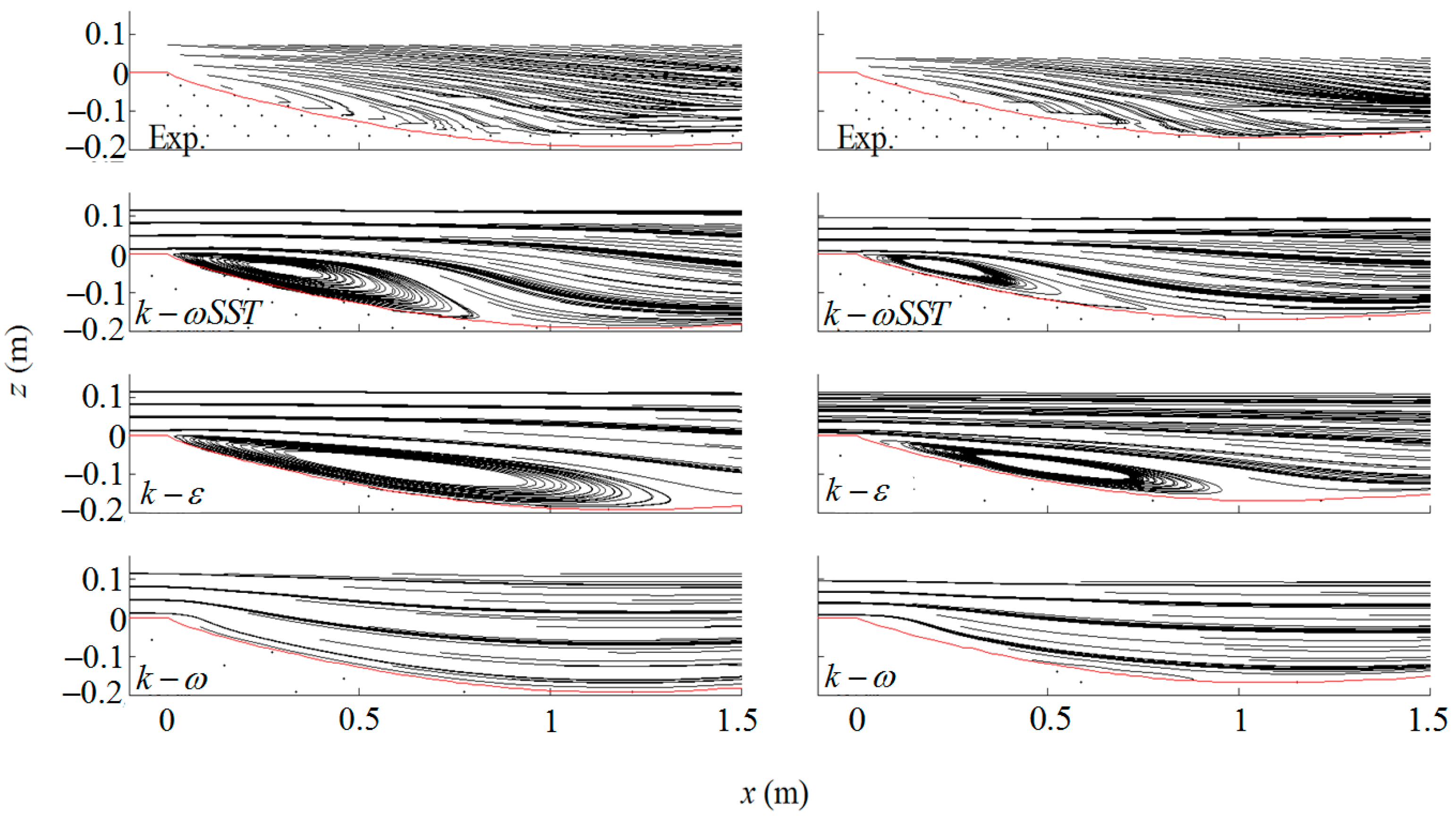
Figure 5.
Velocity profiles along the channel with respect to turbulence models along with the experimental data for Case Exp1 (above) and Case Exp2 (below).
Figure 5.
Velocity profiles along the channel with respect to turbulence models along with the experimental data for Case Exp1 (above) and Case Exp2 (below).
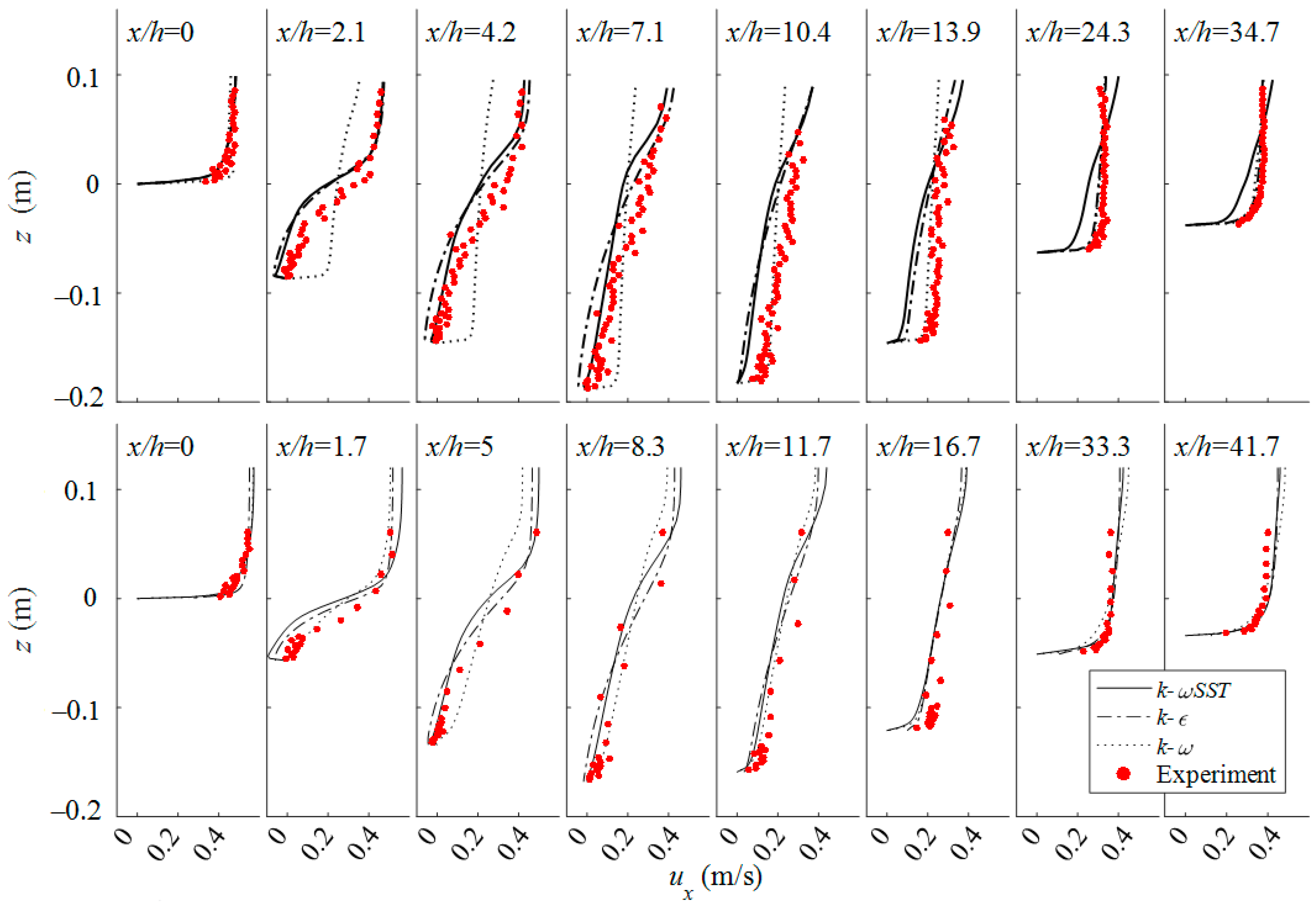
Figure 6.
The wall shear stresses of three models.
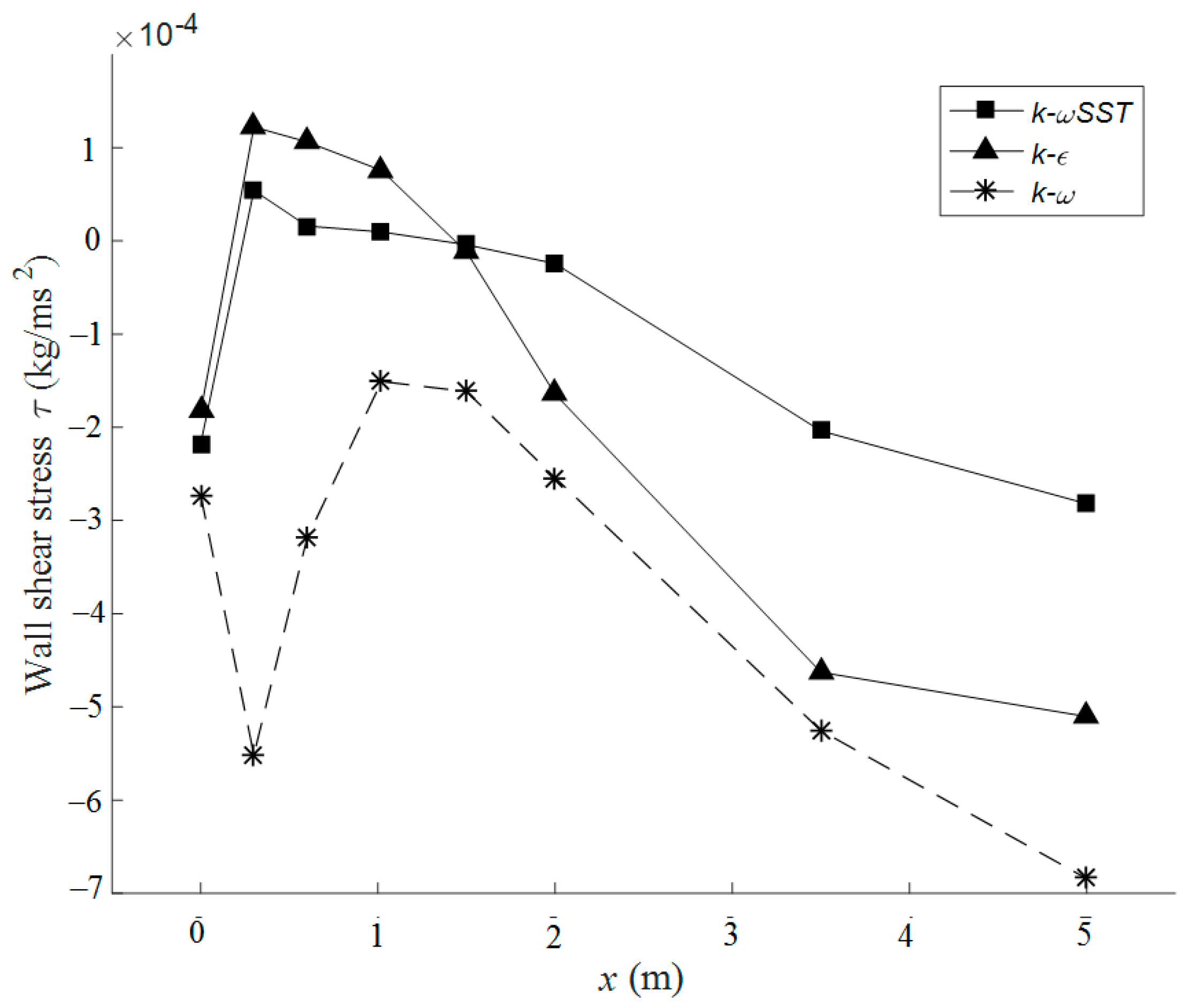
Figure 7.
Turbulence kinetic energy along the channel with respect to turbulence models along with the experimental data for Case Exp1 (above) and Case Exp2 (below).
Figure 7.
Turbulence kinetic energy along the channel with respect to turbulence models along with the experimental data for Case Exp1 (above) and Case Exp2 (below).

Table 1.
Physical experiment set up.
| Case | Q (m3/s) | h (m) | u (m/s) | d50 (m) | Re |
|---|---|---|---|---|---|
| Exp1 | 0.035 | 0.144 | 0.405 | 0.0012 | 58,300 |
| Exp2 | 0.12 | 0.486 | 58,300 |
Table 2.
Experimental constants for the model [17].
Table 2.
Experimental constants for the model [17].
| 1.44 | 1.92 | −0.33 | 0.09 | 1.0 | 1.3 |
Table 3.
Initial model parameters.
| Case | Turbulence Model | Inlet Flow Vel. (m/s) | K (10−2 m2/s2) | (10−9 m2/s3) | (1/s) | (s) | (mm) | |
|---|---|---|---|---|---|---|---|---|
| Min | Max | |||||||
| 0.405 | 1.22 | 3.89 | 10−4 | 1.5 | 10 | |||
| 0.486 | 1.7 | 10.7 | ||||||
| 0.405 | 1.22 | 4.792 | ||||||
| 0.486 | 1.7 | 5.67 | ||||||
| SST1 | 0.405 | 1.22 | 4.792 | |||||
| SST2 | 0.486 | 1.7 | 5.67 | |||||
Table 4.
Accuracy of modeling by root mean square error (RMSE in m/s).
| Physical Case | Case Exp1 | Case Exp2 | ||||
|---|---|---|---|---|---|---|
| Numerical case | 1 | 1 | SST1 | 2 | 2 | SST2 |
| RMSE | 0.0561 | 0.0560 | 0.0407 | 0.0431 | 0.0448 | 0.0413 |
© 2018 by the authors. Licensee MDPI, Basel, Switzerland. This article is an open access article distributed under the terms and conditions of the Creative Commons Attribution (CC BY) license (http://creativecommons.org/licenses/by/4.0/).
Share and Cite
MDPI and ACS Style
Nguyen, T.H.T.; Ahn, J.; Park, S.W. Numerical and Physical Investigation of the Performance of Turbulence Modeling Schemes around a Scour Hole Downstream of a Fixed Bed Protection. Water 2018, 10, 103. https://doi.org/10.3390/w10020103
AMA Style
Nguyen THT, Ahn J, Park SW. Numerical and Physical Investigation of the Performance of Turbulence Modeling Schemes around a Scour Hole Downstream of a Fixed Bed Protection. Water. 2018; 10(2):103. https://doi.org/10.3390/w10020103
Chicago/Turabian StyleNguyen, Thi Hoang Thao, Jungkyu Ahn, and Sung Won Park. 2018. "Numerical and Physical Investigation of the Performance of Turbulence Modeling Schemes around a Scour Hole Downstream of a Fixed Bed Protection" Water 10, no. 2: 103. https://doi.org/10.3390/w10020103
Note that from the first issue of 2016, this journal uses article numbers instead of page numbers. See further details here.