Cross-Analysis of Land and Runoff Variations in Response to Urbanization on Basin, Watershed, and City Scales with/without Green Infrastructures

Abstract

Evaluating land and runoff variations caused by urbanization is crucial to ensure the safety of people living in highly developed areas. Based on spatial scales, runoff analysis involves different methods associated with the interpretation of land cover and land use, the application of hydrological models, and the consideration of flood mitigation measures. Most studies have focused on analyzing the phenomenon on a certain scale by using a single data source and a specific model without discussing mutual influences. In this study, the runoff changes caused by urbanization are assessed and cross-analyzed on three sizes of study areas in the Zhuoshui River Basin in Taiwan, including basin (large), watershed (medium), and city (small) scales. The results demonstrate that, on the basin scale, land-cover changes interpreted from satellite images are very helpful for identifying the watersheds with urbanization hotspots that might have larger runoff outputs. However, on the watershed scale, the resolution of the land-cover data is too low, and land-cover data should be replaced by investigated land-use data for sophisticated hydrological modeling. The mixed usage of land-cover and land-use data is not recommended because large discrepancies occur when determining hydrological parameters for runoff simulation. According to present and future land-use scenarios, the influence of urbanization on runoff is simulated by HEC-1 and SWMM on watershed and city scales, respectively. The results of both models are in agreement and show that runoff peaks will obviously increase as a result of urbanization from 2008 to 2030. For low return periods, the increase in runoff as a result of urbanization is more significant and the city’s contribution to runoff is much larger than its area. Through statistical regression, the watershed runoff simulated by HEC-1 can be perfectly predicted by the city runoff simulated by SWMM in combination with other land/rainfall parameters. On the city scale, the installation of LID satisfactorily reduces the runoff peaks to pre-urbanization levels for low return periods, but the effects of LID are not as positive and are debatable for higher return periods. These findings can be used to realize the applicability and limitations of different approaches for analyzing and mitigating urbanization-induced runoff in the process of constructing a sponge city.

1. Introduction

Along with urbanization, disaster mitigation becomes more and more important with the growth of population, industry, and economic activities. The increase of impervious area in cities reduces water infiltration and soil conservation, thereby increasing the likelihood of flooding and shortening the time to runoff peak [1,2]. Therefore, analyzing the surface runoff variation from land-cover and land-use changes pre- and post-urbanization is crucial when developing flood mitigation measures for urban areas. Research has determined that urbanization greatly influences surface runoff. Liu et al. [3] adopted 4-y rainfall data to calculate surface runoff generated by different land-use classes in the Alzette basin of the Steinsel River, Luxembourg, showing that the urban area occupied only 20% of the total area but generated runoff accounting for 29.3% of the total runoff, whereas other land-use classes (such as farmland and woodland) generated less proportions of runoff even though they cover a larger area. For the Buji River Basin in China, Shi et al. [4] indicated that the runoff peak increased by 13.4% when the urbanized area increased from 2.02 km² (3.5%) in 1980 to 33.58 km² (58.72%) in 2000.

Land-cover and land-use data are different in acquisition and usage. Land cover refers to the area ratio of a region covered by forests, agricultural land, water bodies, or other types of landscapes, whereas land use refers to how an area is used by people (e.g., building, conservation, park). Land-cover changes are usually determined by interpreting multi-period satellite images or remote-sensed data assisted by spatial analysis tools such as GIS (Geographical Information System) for map overlaying [5,6]; this is cost-effective and thus suitable for periodically updating hydrological parameters on a large scale [7,8,9]. Land-use changes cannot be determined from image processing but are determined from a filed survey or the investigation of environmental, economic, and social activities [10,11,12]. Thus, land-use data are often localized and related to policies regulating human activities on a small scale [13,14].

The runoff changes caused by land-use and land-cover variations can be estimated by applying hydrological models that incorporate geographical characteristics. Rainfall-runoff models, such as HEC-HMS (Hydrologic Engineering Center-Hydrologic Modeling System, Army Corps of Engineers, Washington, DC, USA) developed by Hydrologic Engineering Center of the US Army Corps of Engineers [15], are usually coupled with soil infiltration models in conjunction with the GIS to analyze runoff distributions on basin scales [16,17]. The precision of this approach is restricted by the resolution of basin size and can be subject to empirical judgement in translating soil conditions into hydrological parameters. To realize the runoff variation in areas much smaller than a river basin, such as a highly urbanized community or village, the hydrodynamic simulation of rainfall-runoff processes is necessary. A variety of hydrological models, such as the SWMM (Storm Water Management Model, Environmental Protection Agency, Washington, DC, USA), MIKE (Institute for Water and Environment, Horsholm, Denmark), and INFOWORKS (Innovyze,.Conroe, TX, USA, are available for rainfall-runoff analysis in urban areas [18,19]. Among them, models such as SWMM [20] are prevalent for simulating runoff generated by single or continuous rainfall to address water quality and quantity problems related to an urban drainage system. For example, Guan et al. [21] used the SWMM to simulate hydrological changes when an area develops from rural to residential; Xu and Zhao [18] used SWMM to demonstrate that surface runoff increased by 3.5 times in the process of urbanization for a small catchment in Beijing (Liangshui River Basin, 131 km²).

In the last two decades, the idea of “sponge city” has been put into practice in the United Sates [22], the United Kingdom [23], Canada [24], Australia [25], and other countries by designing low-impact, green, and sustainable urban drainage systems in highly urbanized areas. The purpose of sponge city is to reduce stormwater runoff, restore the ecological environment, and preserve natural resources through land-use changes that increase absorption, storage, and purification of rainwater [26,27,28]. To construct a sponge city, many researchers have suggested that the green infrastructure, also called LID (Low Impact Development) approach, is more efficient than traditional systems in reducing initial runoff [28,29,30,31]. The SWMM is recommended as the most suitable tool for evaluating the performance of LID facilities [32,33,34,35].

From the aforementioned literature review, runoff variations and mitigation in response to land-use and land-cover changes caused by urbanization have been widely studied. However, depending on the research objective, most studies have analyzed the phenomenon either on a large basin scale or on a small city scale by using specific land data and hydrological models. An overall study of the influences of urbanization on runoff across data, models, and scales has not been conducted. Therefore, certain questions require to be answered, for example, (a) is it appropriate to mix land-cover and land-use data for hydrological analysis? (b) how do hydrological models affect runoff results when the same land data are input? and (c) how do LID approaches benefits flood mitigation on different spatial scales? The purpose of this study is to assess and cross-analyze land and runoff changes on basin (large), watershed (medium), and city (small) scales in the Zhuoshui River Basin in Taiwan. On the basin scale, the historical land-cover and runoff changes are analyzed through the classification of satellite images and the application of the HEC-1 model. On the watershed scale, sub-basins with a higher degree of urbanization are pinpointed, and the results from the other two scales are accumulated and cross-analyzed. On the city scale, runoff changes under present and future land-use scenarios with and without LID measures are quantified through the application of SWMM. The procedure enables a comprehensive test of the applicability and limitation of relevant methodologies and provide valuable information for future studies.

2. Study Areas

On the basin scale, the Zhuoshui River Basin is selected as the study area. It is located in central Taiwan and has the longest mainstream of 187 km and the second largest catchment of 3157 km² in Taiwan. The Zhoushui River originates from the Hehuan Mountain at an attitude of 3220 m and flows westward into the Taiwan Strait while converging with many tributaries that divide the entire river basin into 21 watersheds, as revealed by geographical processing. Among these watersheds, the watershed located at the intersection of the Zhoushui River and its tributary the Qingshui River, is selected as the medium-scale study area where an aggregation of artificial structures has been observed. Lying in the middle of the selected watershed, the Jushan urban planning district is further selected as the smallest study area for city-scale land and runoff analyses. Urban planning for Jushan was first formulated under the Japanese colonial rule in 1917, although the initial content was nothing but a simple road construction project covering 53.8 hectares. In 1979, the urban planning area was expanded to 418.1 hectares and has been subsequently revised a total of 13 times since then [36]. Figure 1 illustrates the study areas on basin scale, watershed, and city scales.

3. Methodology

In this study, based on the scales of the study areas, different data, models, and time periods are employed for analysis of land and runoff variations, which are listed in

Table 1. Study subjects on different scales.

Subject	Basin	Watershed	City
Land Data	Land-cover	Land-cover/Land-use	Land-use
Runoff Model	HEC-1	HEC-1	SWMM
Time Period	History	History/Present/Future	Present/Future/Future with LID

and described in the following paragraphs. In the table, the runoff models are chosen according to their applicability. The SWMM is developed for simulating water quantity and quality in urban areas with drainage systems, in which the rainfall-runoff process is determined by methods suitable for small catchments. The HEC-1 (Hydrologic Engineering Center-1, Army Corps of Engineers, Washington, DC, USA) model is designed for surface runoff simulation on a river basin scale without considering drainage systems. Compared with SWMM, the HEC-1 has more options on the methods describing the processes of evaporation, infiltration, rainfall accumulation, and runoff routing.

3.1. Basin Scale

To determine the land-cover change for the Zhoushui River Basin, historical ortho-images taken by the satellite FORMOSA II are adopted for analysis. The FORMOSA II is a sun-synchronous satellite located at an attitude of 891 km above the ground surface, and it provides high-resolution images (2 m for black/white images and 8 m for multi-spectral color images) twice a day for Taiwan area. The satellite images from 1998 to 2013 are collected and divided into smaller segments for interpreting and extracting land-cover characteristics. Using an object-oriented classification method (i.e., SVM, Support Vector Machine [37]), 15 image indexes including NDVI (Normalized Difference Vegetation Index), SAVI (Soil Adjusted Vegetation Index), mean Brightness, mean Blue, mean Red, mean Green, mean NIR (mean Near Infrared), std. Blue, std. Red, std. Green, std. NIR (standard deviation Near Infrared), pix-base Blue, pix-base Red, pix-base Green, and R to RGB (Red, Green, Blue) are identified for classifying the land-cover into four types: water, built-up land, bare land, and vegetation. The classification results are then displayed by the area transfer matrix to investigate land-cover changes between each period [38].

The urbanization level is measured by determining whether an aggregation of artificial structures is present in the Zhoushui River Basin through Spatial Autocorrelation Analysis (SAA) [39] and Spatial Hotspot Analysis (SHA) [40]. The SAA uses the Moran’s I and Z-score [41] as indexes to estimate the significance of homogeneity in structure distributions. If an area has a value of Moran’s I > 0 with a Z-score > 1.96, the hypothesis of structure aggregation will be accepted under 5% of significance level. Once the SAA confirms the pattern of structure aggregation, the SHA employs the $G_i$ index defined by Getis and Ord [42] to determine the hotspots of these artificial structures. The more the $G_i$ exceeds 0, the higher the structure aggregation level in an area.

After completing the interpretation of land-cover change, the HEC-1 model, developed by the US Army Corps of Engineers [43], is employed for runoff simulation on the basin scale for different periods. Being a lumped model, the HEC-1 divided the whole basin into various watersheds connected to each other by channel networks, in which the runoff is transported in the forms of overland flow and channel flow depending on topographical characteristics. The watershed divisions are determined by processing DEM (Digital Elevation Model) data on a GIS platform. The CN (Curve Number) method proposed by US Soil Conservation Service (SCS) [44] is employed to estimate infiltration losses for determining the effective rainfall substituted into the HEC-1 for runoff simulation. The CN is an empirical value that increases with impermeability; thus, it is a suitable parameter that reflects urbanization level. The CN values for the four types of land-cover determined earlier are referred to in the table summarized in the SCS technical book [44].

3.2. Watershed Scale

In addition to historical land-cover changes discovered from the satellite images, present and future land-use scenarios are investigated on the watershed scale. The national land-use survey data obtained by the National Land Surveying and Mapping Center of Taiwan in 2008 [45] are selected as the present land-use scenario. The designed land uses in 2030, which are illustrated in the urban planning project proposed by the Nantou County government in Taiwan [36], are adopted as future scenario. Because these scenarios are based on official materials, they are in some ways more realistic than model predictions when considering social and economic influences. The investigated land-use scenarios are then put into the HEC-1 model for calculating present and future runoff variations. Thus, on the watershed scale, the land-runoff relationships are determined for the past, present, and future.

3.3. City Scale

On the city scale, runoff changes induced by land-use development, relocation, and renewal are more localized and rapidly changing; therefore, they require more sophisticated hydrodynamic models. The SWMM (ver. 5.1 with LID module) developed by the US Environmental Protection Agency is adopted for runoff simulation on the city scale. In response to a possible increase in runoff due to urban development, flood mitigation measures based on the concept of LID are introduced. Common LID techniques include permeable pavements, green roofs, rain gardens, bio-retention cells, tree box filters, grass swales, infiltration gutters, and rain barrels. Permeable pavements are porous layers that increase the infiltration and evaporation of surface water; green roofs use vegetation planted on roofs to reduce surface runoff and delay the occurrence of runoff peak; rain gardens and bio-retention cells use landscaping and plants to create retention pools that accumulate stormwater for small areas; tree box filters collect runoff from curbside entrances to store and filter water through plants before discharging it into sewer systems; grass swales or infiltration gutters are ditches with grass or permeable covers that increase infiltration while transporting runoff; and rain barrels are small rainwater harvesting systems that collect and retain rainfall water from roofs. In this study, various LID measures are installed based on their applicability.

4. Results and Discussion

4.1. Land-Cover and Runoff Changes on the Basin Scale

Table 2. Changes in land-cover areas against time on basin scale.

Land-Cover Types	1998 (ha)	2003 (ha)	2008 (ha)	2013 (ha)	1998–2013 Change Ratio
Water	12,264	12,284	12,170	12,173	−0.74%
Built-up Land	1990	2792	2802	3023	51.91%
Bare Land	8551	9650	14,561	10,347	21.00%
Vegetation	277,445	275,524	270,717	274,707	−0.99%

summarizes the areas of water, built-up land, bare land, and vegetation in 1998, 2003, 2008, and 2013. Area changes for vegetation and water are not significant in terms of ratio because approximately 91.5% of the total land is covered by vegetation, 4% by water, 3.5% by bare land, and only 1% by built-up land. The built-up area showed a constant increase from 1990 hectares in 1998 to 3023 hectares in 2013, with a total increase of 51.91%. The area of bare land slightly increased from 8551 hectares in 1998 to 9650 hectares in 2003, and substantially increased to 14,561 hectares in 2008, followed by a decrease to 10,347 hectares in 2013, resulting in a total increase of 21% from 1998 to 2013. In contrast, the area covered by vegetation had the opposite pattern by decreasing constantly from 277,445 hectares in 1998 to 270,717 hectares in 2008 before subsequently increasing to 274,707 hectares in 2013. This finding indicates that there was a switch between the bare land and vegetation land from 1998 to 2013.

Table 3. Land-cover transfer matrix from 1998 to 2003.

	1998	Water (ha)	Built-Up Land (ha)	Bare Land (ha)	Vegetation (ha)	Total (ha)	1998–2003 Change Ratio
2003
Water		11,209	86	376	614	12,284	0.16%
Built-up Land		80	1637	248	827	2792	40.28%
Bare land		237	66	3074	6273	9650	12.84%
Vegetation		738	201	4854	269,731	275,524	−0.69%
Total		12,264	1990	8552	277,445	300,250

,

Table 4. Land-cover transfer matrix from 2003 to 2008.

	20003	Water (ha)	Built-Up Land (ha)	Bare Land (ha)	Vegetation (ha)	Total (ha)	2003–2008 Change Ratio
2008
Water		11,935	77	85	73	12,170	−0.93%
Built-up Land		137	2249	30	386	2802	0.37%
Bare Land		98	82	4211	10,170	14,561	50.89%
Vegetation		114	384	5324	264,895	270,717	−1.74%
Total		12,284	2792	9650	275,524	300,250

,

Table 5. Land-cover transfer matrix from 2008 to 2013.

	2008	Water (ha)	Built-Up Land (ha)	Bare Land (ha)	Vegetation (ha)	Total (ha)		2008–2013 Change Ratio
2013
Water		12,024	22	25	102		12,173	0.03%
Built-up Land		16	2208	275	524		3023	7.87%
Bare Land		92	330	8253	1673		10,347	−28.94%
Vegetation		38	242	6008	268,419		274,707	1.47%
Total		12,170	2802	14,561	270,717		300,250

and

Table 6. Spatial autocorrelation of artificial structures from 1998 to 2013.

Index	1998	2003	2008	2013
Moran’s I	0.67	0.76	0.60	0.63
Z-score	94.90	98.20	103.92	118.60
p-value	0.00	0.00	0.00	0.00

display the land-cover transfer matrixes between 1998–2003, 2003–2008, and 2008–2013, respectively. From Table 3, the increase in built-up land, with a peak increase of 40.28% from 1998 to 2003, can be attributed to construction on vegetation land and bare land. Moreover, the increase in bare land displayed in Table 3 and Table 4 is a result of the deterioration of vegetation land, particularly from 2003 to 2008 when 10,170 hectares of vegetation land were converted into bare land. However, in Table 5, a rapid recover of vegetation land from bare land between 2008 and 2013 is seen, with 6008 hectares of bare land being transformed into vegetation land. These phenomena can be explained by the occurrence of a devastating earthquake in 1999, with its epicenter located in the Chi-Chi area in the study river basin. During the Chi-Chi earthquake, slope lands became weaker and unstable, causing collapses and landslides that washed away vegetation covers in the typhoon seasons of the following 10 years. The recovery of vegetation land between 2008 and 2013 indicates that the slope land has regained stability. The significant increase in the built-up area between 1998 and 2003 can also be attributed to the Chi-Chi earthquake owing to the relocation and reconstruction of the buildings destroyed in the disaster. Thus, in the study area, the occurrence of a major earthquake speeds up urbanization by forcing more undeveloped land to become built-up areas.

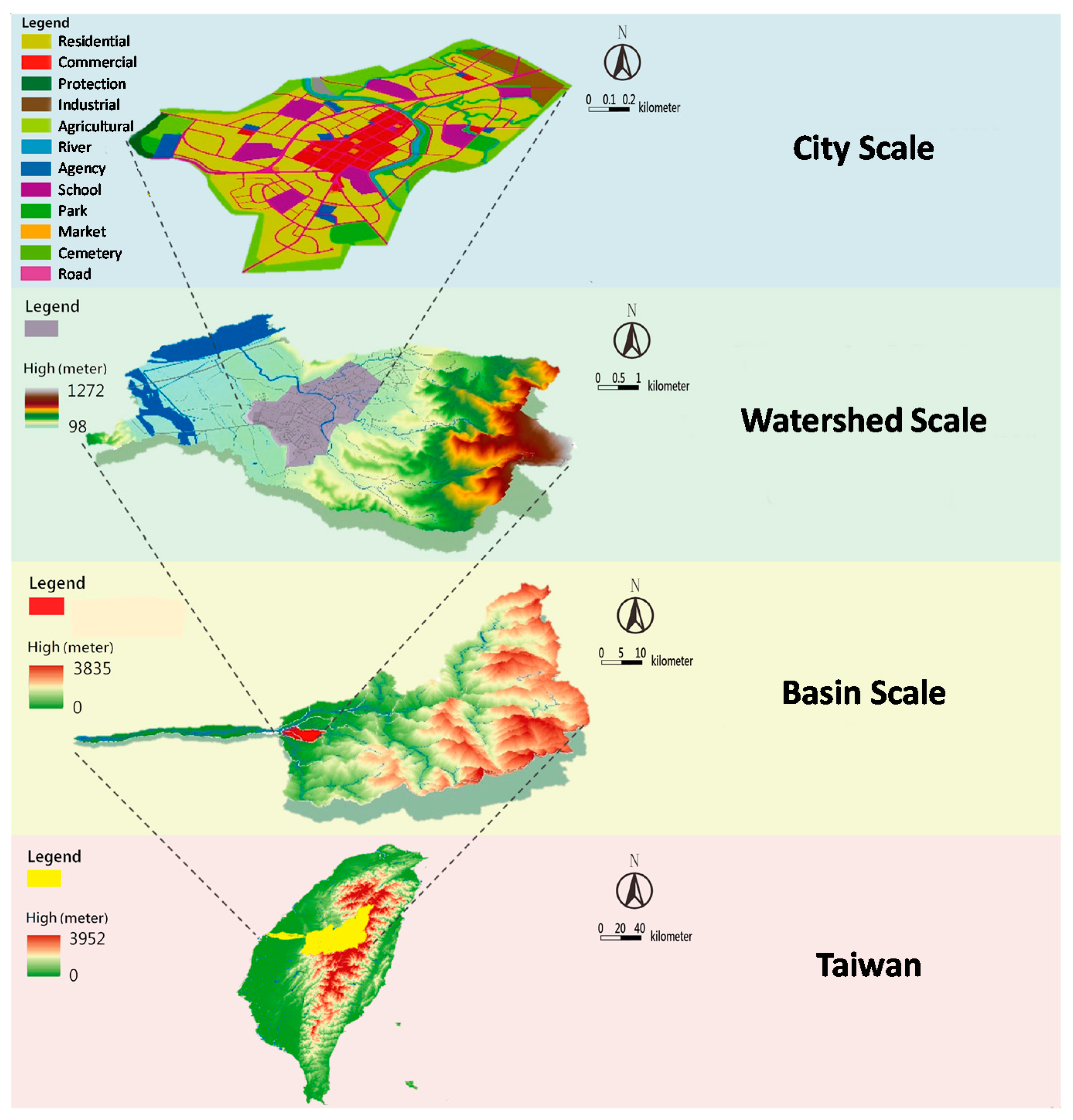
To determine the spatial aggregation of artificial structures in the Zhuoshui River Basin, SAA is conducted in grid units with a resolution of 500 m. Table 6 lists the Moran’s indexes, Z-score, and p-value for 1998, 2003, 2008, and 2013. With all Moran’s I > 0, Z-scores > 2.58, and p-values ~ 0, it demonstrates that the artificial structures in Zhoushui river basin are not distributed randomly in space, but are highly accumulated. 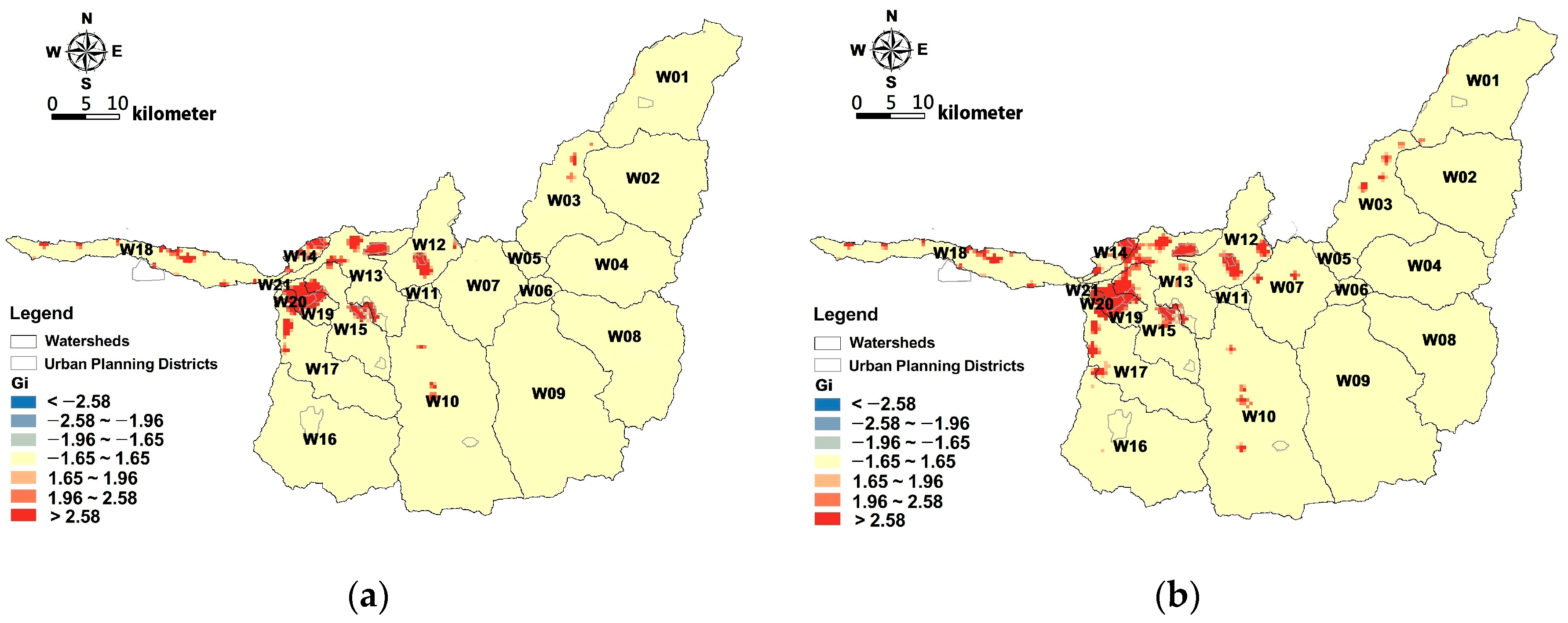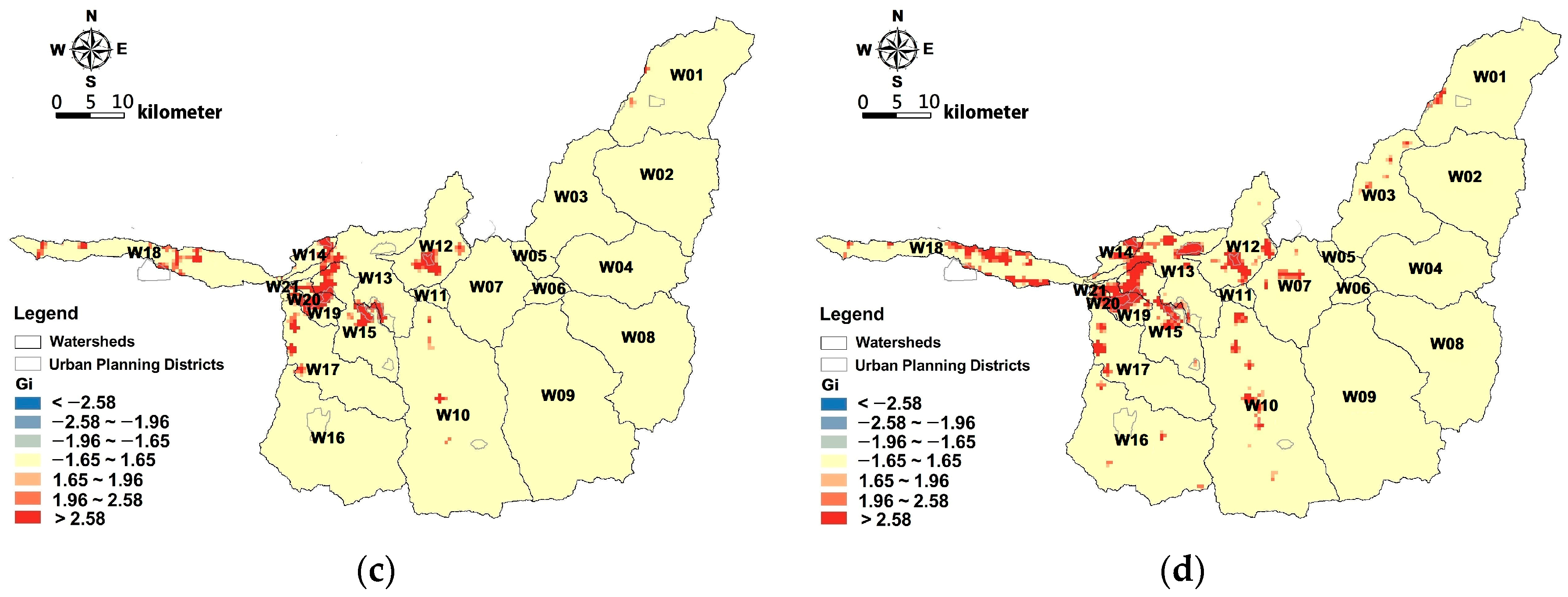Figure 2 shows the hotspots of the artificial structures in 1998, 2003, 2008, and 2013, in which the grey lines are the boundaries of the 21 watersheds and the red color denotes the grids with higher $G_i$ (Getis) values. The hotspots of artificial structures were concentrated in the watersheds around the bottleneck between the upstream catchment and the downstream river channel, particularly in watersheds numbered W19 and W20, which are thus chosen as the subjects for the medium-scale studies.

To initiate the HEC-1 model for runoff simulation, the 24-h rainfall amounts under different return periods are obtained from frequency analysis based on the historical records of the Chi-Chi rain station. The 24-h rainfall amounts under 2-, 5-, 25-, 50-, and 100-y return periods are 204.61, 308.29, 473.97, 543.38, and 612.50 mm, respectively. The rainfall hyetographs served for runoff simulation are determined by the intensity-duration-frequency relationships suggested by Horner and Flynt [46] according to the design handbook published by the Water Resource Agency, Taiwan [47].

Table 7. Parameters for HEC-1 model.

Watershed	Area (km2)	Length-W (m)	Slope-W	Length-C (m)	Slope-C	Roughness-W	n-C
W01	222.84	2328	0.63	47,855	0.05	0.20	0.02
W02	223.20	2619	0.61	42,612	0.05	0.20	0.02
W03	159.35	1665	0.65	47,856	0.05	0.20	0.02
W04	167.32	1836	0.66	45,557	0.06	0.20	0.02
W05	21.16	306	0.71	34,579	0.02	0.20	0.02
W06	19.20	1101	0.73	8721	0.19	0.20	0.02
W07	144.80	5708	0.66	12,684	0.08	0.20	0.02
W08	255.09	2924	0.65	43,617	0.06	0.20	0.02
W09	416.28	23,867	0.72	8721	0.19	0.20	0.02
W10	434.60	4840	0.65	44,893	0.08	0.20	0.02
W11	13.70	1089	0.45	6312	0.15	0.20	0.02
W12	111.10	1808	0.39	30,739	0.03	0.20	0.02
W13	125.60	2044	0.27	30,739	0.03	0.20	0.02
W14	19.40	562	0.09	17,291	0.02	0.20	0.02
W15	102.10	1982	0.38	25,752	0.07	0.20	0.02
W16	269.90	3546	0.57	38,056	0.06	0.20	0.02
W17	141.00	8741	0.46	8065	0.02	0.20	0.02
W18	117.60	1282	0.02	45,867	0.01	0.20	0.02
W19	26.70	1657	0.19	8065	0.02	0.20	0.02
W20	7.60	468	0.06	8065	0.02	0.20	0.02
W21	2.40	282	0.11	4318	0.05	0.20	0.02
W23	0.15	276	0.07	270	0.01	0.20	0.02

Note: Length-W: representative length of watershed; Slope-W: representative slope of watershed; Length-C: representative length of channel; Slope-C: representative slope of channel; Roughness-W: overland-flow roughness coefficient; n-C: Manning’s n for channel.

lists the parameters for the HEC-1 model and

Table 8. Variations of CN, IMP, and $Q_p^{100}$ related to land-cover and land-use changes on different study scales.

Index	Land-Cover				Land-Use
	1998	2003	2008	2013	2008	2030
Basin scale
Zhuoshui Basin (316,800 ha)
CN	43.42	44.17	44.64	44.09
IMP (%)	0.53	0.62	0.69	0.79
$Q_p^{100}$ (cms)	48,835	49,350	49,379	49,446
Watershed scale
W19 (2673 ha)
CN	51.45	53.18	51.34	52.20	60.55	62.31
IMP (%)	12.91	13.13	14.05	15.00	14.12	18.76
$Q_p^{100}$ (cms)	416	422	417	424	467	486
W20 (755 ha)
CN	65.38	64.14	63.63	64.92	69.75	76.48
IMP (%)	7.29	8.66	8.79	9.64	13.50	14.73
$Q_p^{100}$ (cms)	182	181	182	183	188	198
City scale
Jushan Dist. (422 ha)
IMP (%)					45.78	61.80
$Q_p^{100}$ (cms)					79.62	84.26

summarizes the CN, the area ratio of impermeability (IMP), and 100-y peak runoff discharge ($Q_p^{100}$) on different scales. Overall, no significant changes are observed in CN, IMP, and $Q_p^{100}$ on the basin scale. This may be due to the fact that the land-cover are classified into four groups only, with vegetation land accounting for 91.5% of the total land, which limits the variation of CN and consequent runoff. Table 8 also indicates that, because the W20 watershed has higher values of CN and IMP, it generates runoff of $0.24\mathrm{cms}/\mathrm{ha}$, which is much higher than the basin average $0.16\mathrm{cms}/\mathrm{ha}$.

4.2. Land-Cover, Land-Use, and Runoff Changes on the Watershed Scale

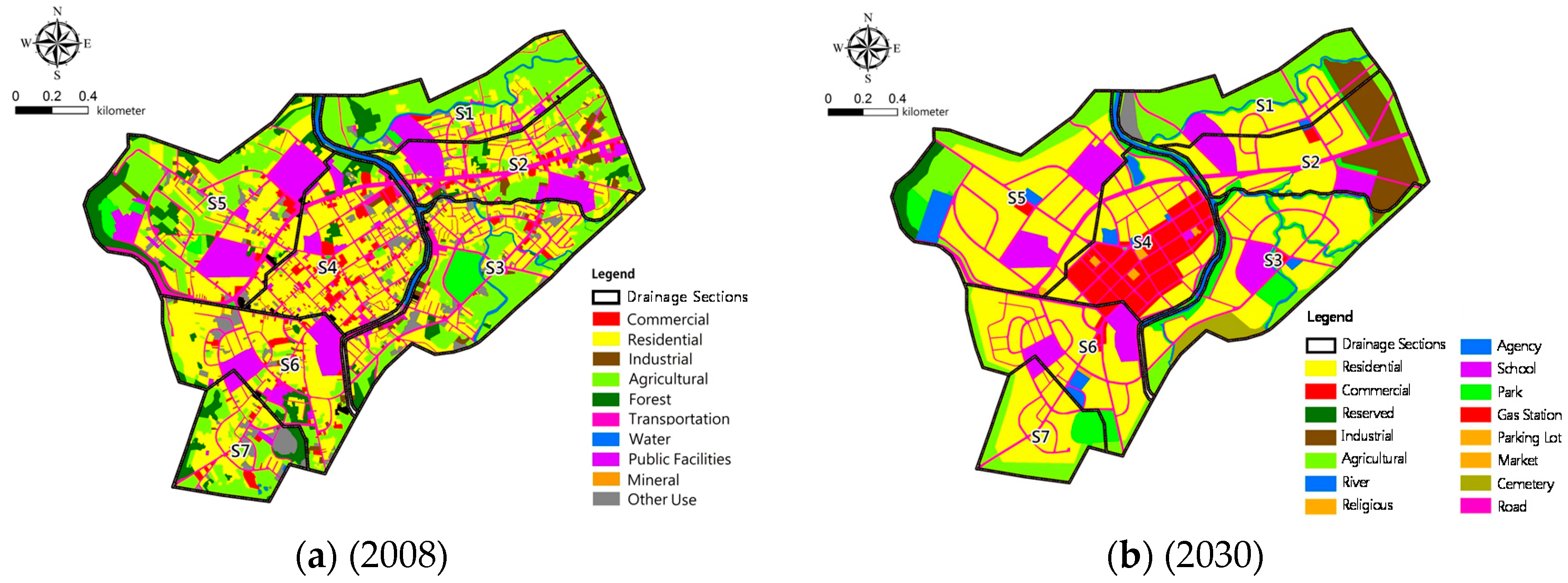
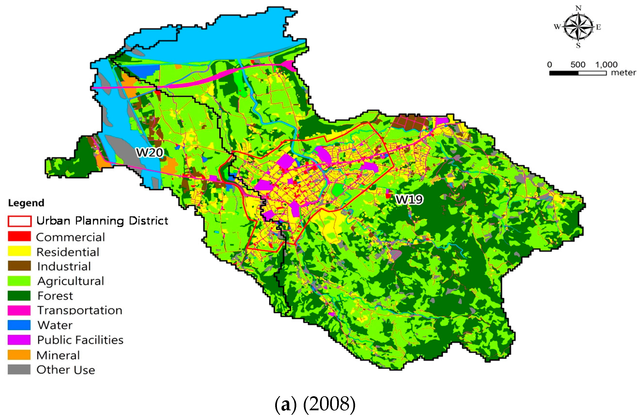
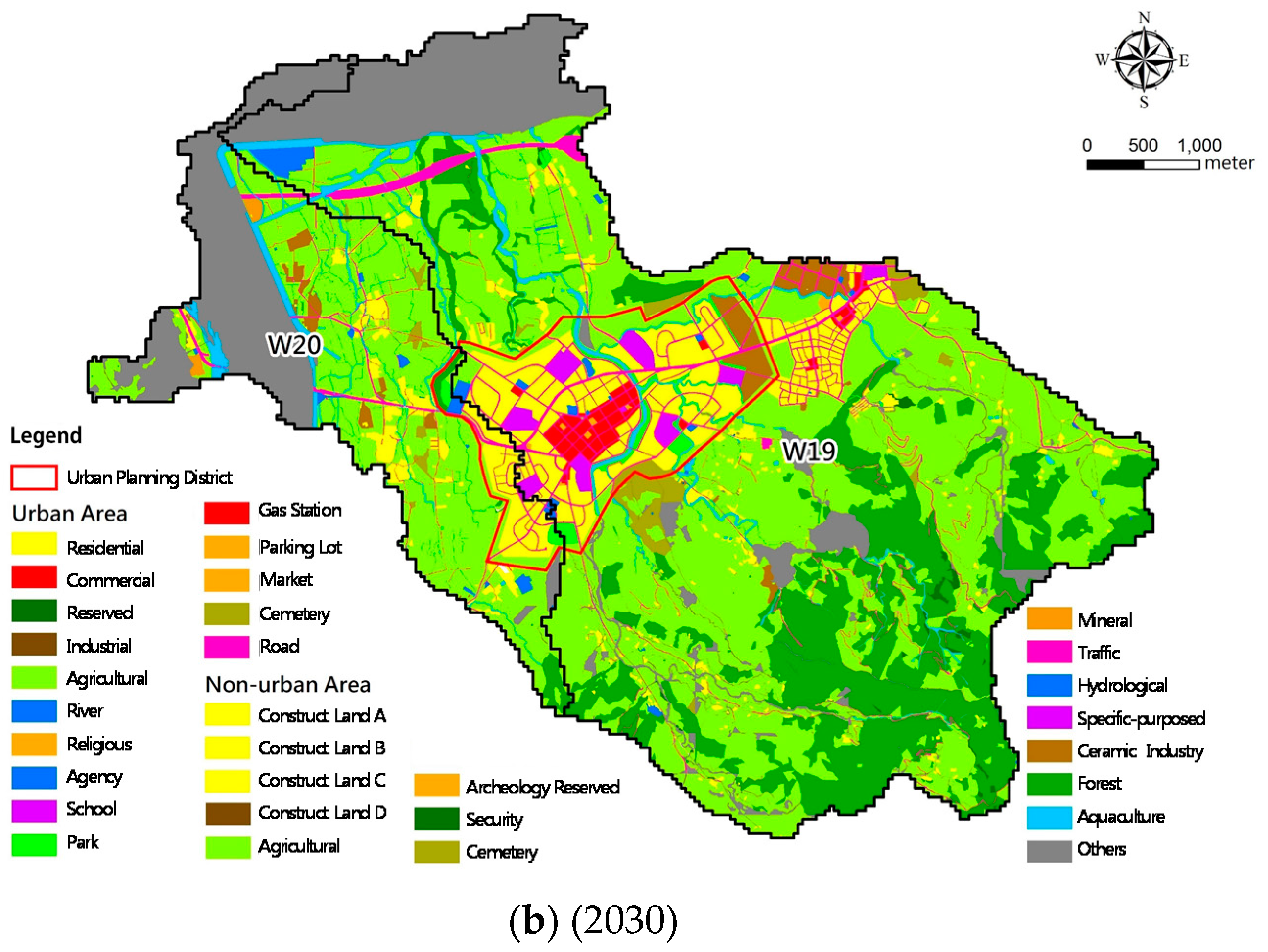
Present (2008) and future (2030) land-use maps on the watershed scales for W19 and W20 are illustrated in Figure 3. Current land uses are divided into 11 categories, and the future land uses are further refined into 32 categories. By 2030, large areas of forests are set to be transformed into agricultural land and many residential regions will be converted into commercial areas. According to land-use changes from 2008 to 2030, for W19, the CN values increase from 60.55 to 62.31, and the IMP increase from 14.12% to 18.76%; for W20, the CN values increase from 69.75 to 76.48, and the IMP increase from 13.50% to 14.73%, as listed in Table 8. However, in the overlay year of 2008, the CN values interpreted from land-use data are much larger than those interpreted from land-cover data (equal to 51.34 for W19 and 63.63 for W20), which can lead to different runoff estimations. These discrepancies are not surprising and can be attributed to the difference in land classification, as 11 types of land-uses exists but only four types of land-covers are classified. This finding indicates that uncertainty analysis should be performed if different sources of land data are incorporated for hydrological analysis; otherwise, their results should be regarded separately. In this paper, runoff variations resulted from land-cover and land-use changes are separately discussed.

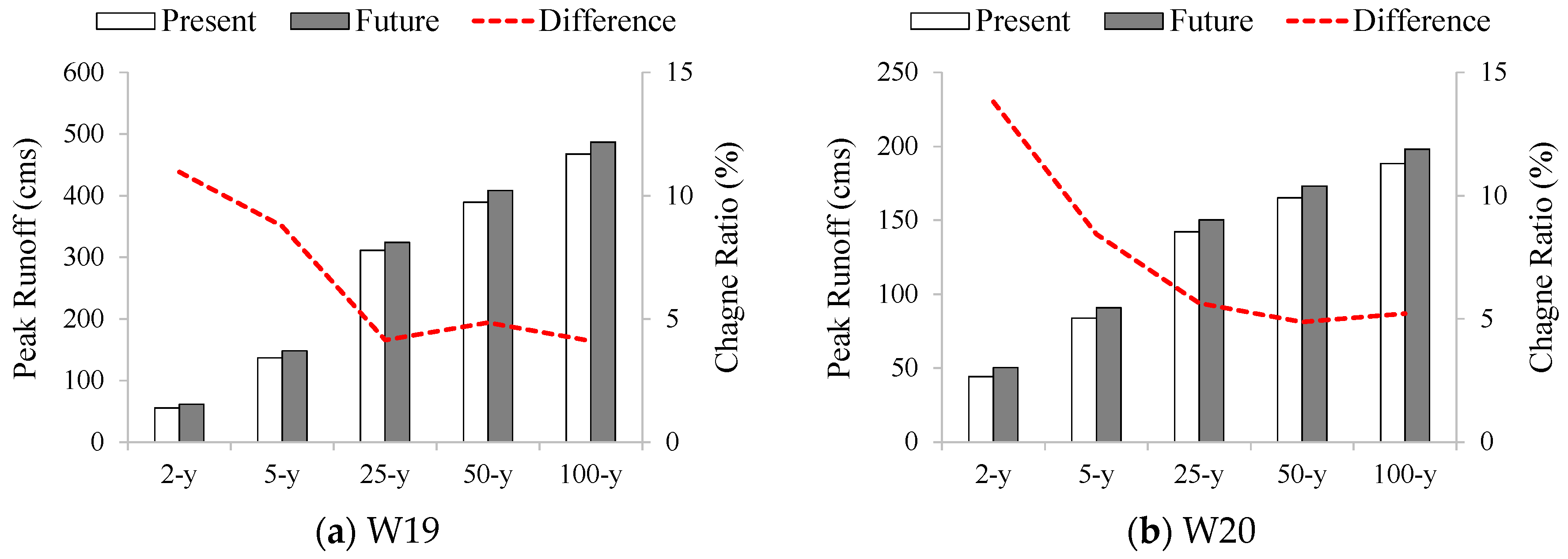
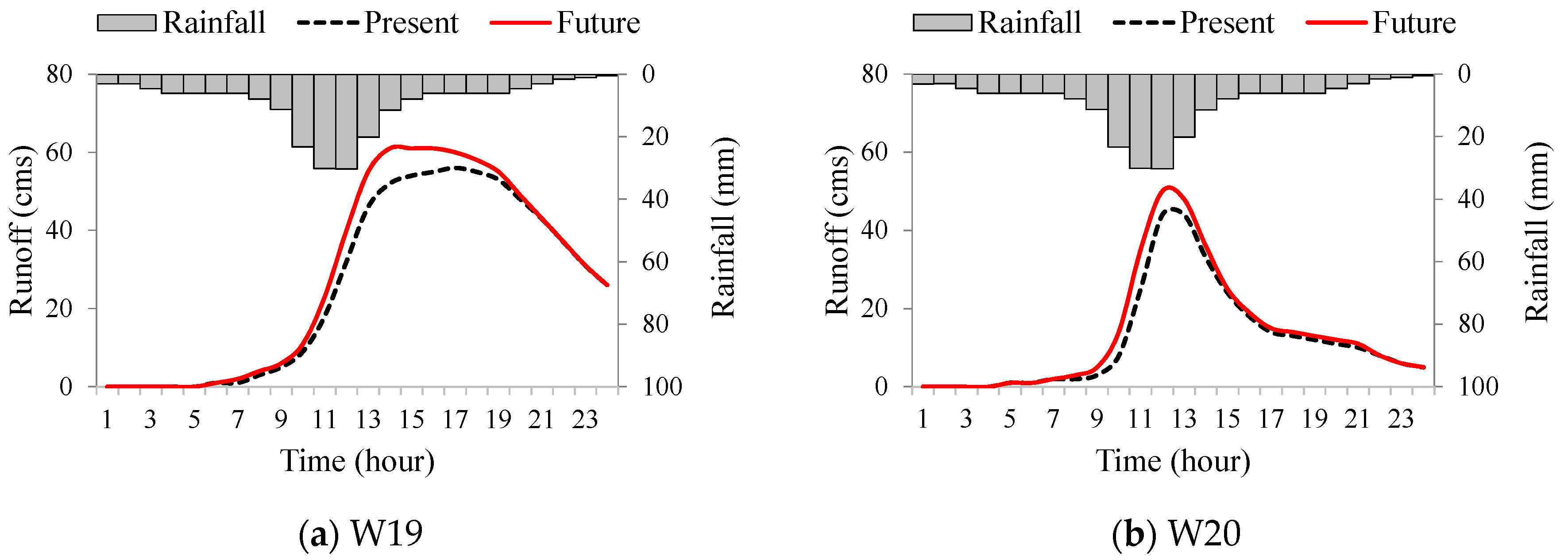
Figure 4 shows a comparison of present and future runoff peaks under different return periods for W19 and W20, respectively. Peak runoff are demonstrated to increase in the future under all return periods for both W19 and W20. Although the increments of peak runoff are smaller at low return periods, their change ratios are instead larger. For both watersheds, the peak runoff under 2-y return periods increase by more than 10% and then drop to a level of 5% under return periods larger than 25 years. The runoff hydrographs under 2-y return period for W19 and W20 are displayed in Figure 5, showing that future runoff peaks not only increase but also shift forward; the integration of runoff hydrographs against time shows that the total increases in runoff volume are 212,400 m³ and 140,400 m³ for W19 and W20, equivalent to 85 and 56 standard swimming pools, respectively. Such an increase presents a non-negligible extra risk of flooding if additional flood control measures are not implemented.

4.3. Land-Use and Runoff Changes on the City Scale

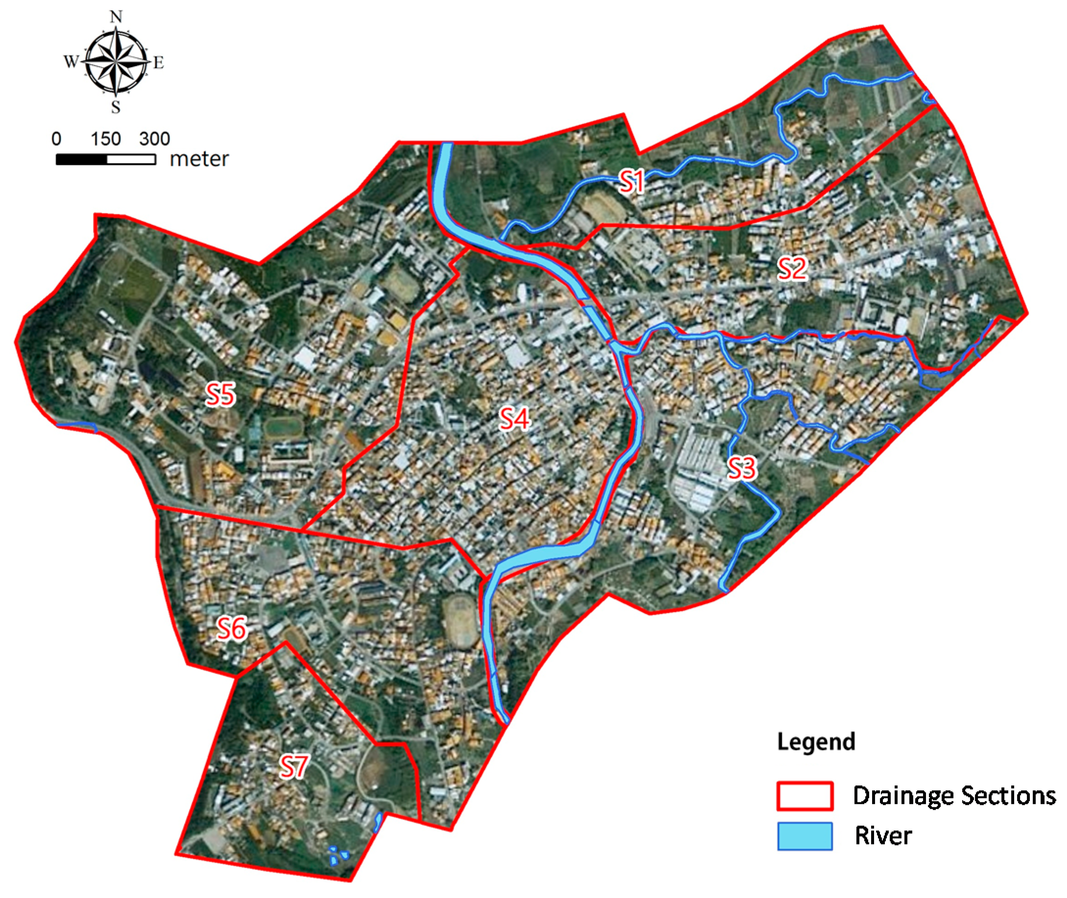
According to the sewer system report for Jushan in 2008 [48], the Jushan District is divided into seven drainage sections as shown in Figure 6 and the land-use maps for these sections at present and in the future are compared in Figure 7. The figure indicates that, by 2030, the commercial area will greatly expand and will be mostly concentrated in S4; a large industrial block will be developed at the borders of S1 and S2; and the residential areas will be increased in almost every section. 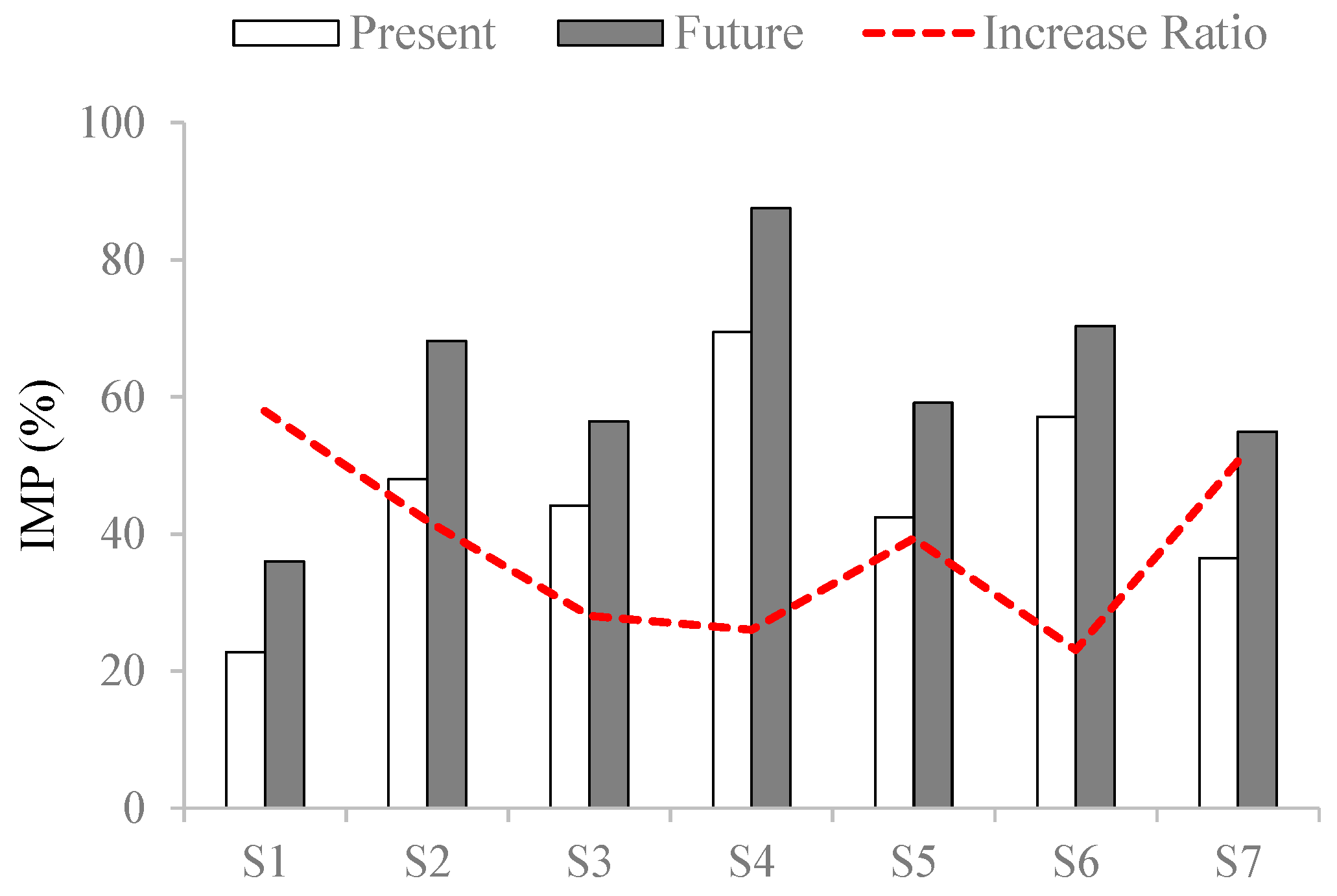Figure 8 indicates that the IMP for all the seven sections increase simultaneously, from 23–69% at present to 36–88% in the future, in which the S1 has the highest increase of $58\%$. The variations of average IMP and $Q_p^{100}$ on the city scale are also listed in Table 8, which shows that this increased IMP will raise $Q_p^{100}$ from 79.62cms to 84.26cms by 2030.

Table 9. Parameters for SWMM.

Drainage Section	Area (ha)	Slope (%)	n-Imp	n-Per	S-Imp (mm)	S-Per (mm)
S1	48.84	0.7	0.01	0.1	0.05	0.05
S2	57.7	0.7	0.01	0.1	0.05	0.05
S3	69.45	0.7	0.01	0.1	0.05	0.05
S4	58.96	1.45	0.01	0.1	0.05	0.05
S5	92.76	1.45	0.01	0.1	0.05	0.05
S6	54.44	1.45	0.01	0.1	0.05	0.05

Note: n-Imp: Manning’s n for impervious land; n-Per: Manning’s n for pervious land; S-Imp: depression storage for impervious land; S-Per: depression storage for pervious land.

summarizes the parameters for SWMM.

In response to the increasing of flood risk, various LID measures are designed and incorporated into the SWMM on the city scale to evaluate their effectiveness of runoff reduction. To reduce public resistance, the LID measures are installed on government-owned lands or facilities. Some lands or facilities such as cemeteries, sewage treatment plants, and gas stations are discounted for LID because of their particular usages.

Table 10. Area ratios of different LID facilities with respect to land-uses.

Land-Use Types	Area (ha)	Bio-Retention Cell (%)	Rain Garden (%)	Green Roof (%)	Infiltration Gutter (%)	Permeable Pavement (%)
School	29.03	-	10	30	15	5
Park	11.82	90	-	-	-	-
Agency	7.17	35	-	50	-	-
Social	7.17	-	-	30	15	5
Market	0.95	-	10	80	-	-
Tourist	0.66	35	-	50	-	-
Parking Lot	0.58	-	35	-	-	-
Plaza	0.29	-	35	-	-	-

summarizes the areas of different land-uses and the area ratios in which different LID facilities are installed. Rain gardens and bio-retention cells are installed in less built-up areas such as parks, parking lots, and plazas, while green roofs are mainly set up on the tops of markets, agencies, and schools. Using the LID control editor built in the SWMM, parameters of the LID facilities are given by different ground layers including surface, soil, and storage, as summarized in

Table 11. Parameters for LID facilities.

Item		Bio-Retention Cell	Rain Garden	Green Roof	Infiltration Gutter	Permeable Pavement
Surface	Berm Height (m)	0.15	0.15	0.04	-	-
Soil	Thickness (m)	0.45	0.45	0.10	-	0.25
	Porosity	0.25	-	0.30	-	0.25
Storage	Thickness (m)	0.15	-	-	0.10	0.45
	Void Ratio	0.25	-	-	0.25	0.25

. The surface and soil layers are porous, allowing water to pass through; the storage layer contains water within the soil void and when the storage is full, excessive water will overflow. In this study, no underdrains are considered. The IMP for each drainage section is adjusted for runoff simulation according to the area occupied by each LID facility.

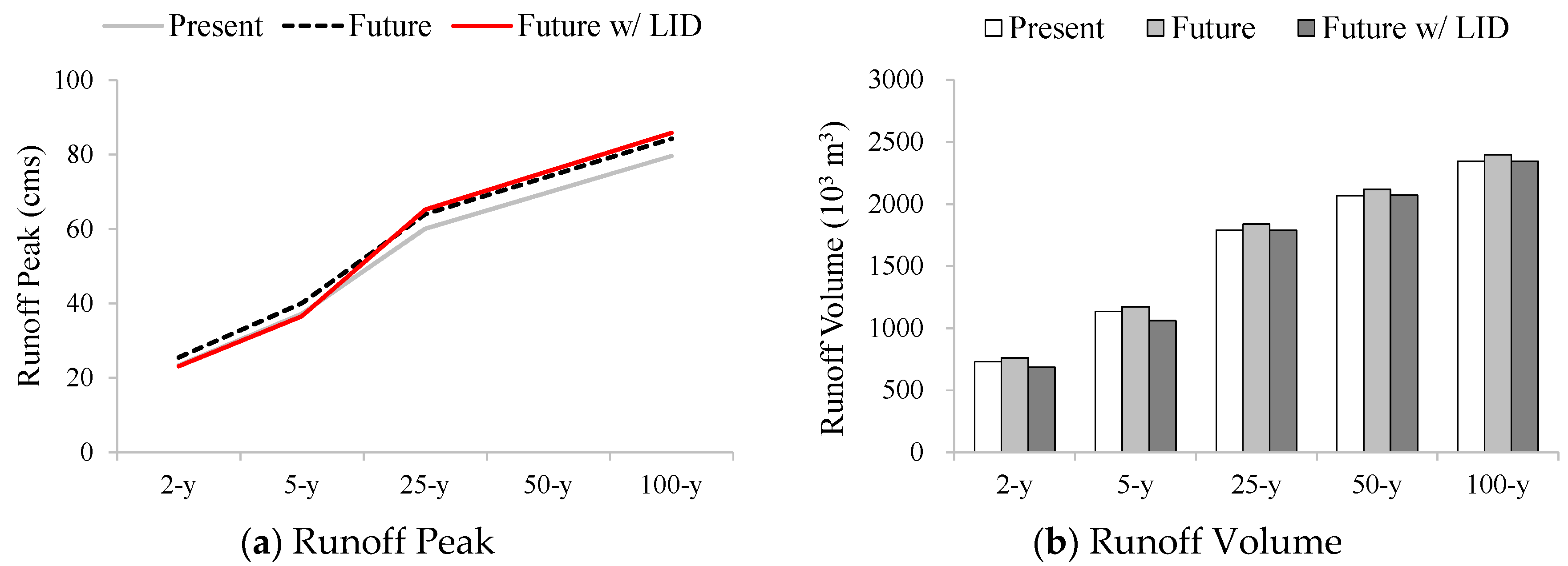
Figure 9 shows the simulated runoff peaks and runoff volumes for different return periods under three land-use scenarios: present, future, and future with LID. Without LID, the runoff peaks and runoff volumes are found to increase simultaneously for all return periods due to the increase in IMP in future urban planning. The increased amounts at high return periods are slightly larger than those at low return periods, but not obvious. After introducing the LID facilities, Figure 9a shows that the runoff peaks for 2-y and 5-y return periods will be effectively reduced to a level even less than the present condition. However, for the 25-, 50-, and 100-y return periods, the introduction of LID instead leads to slight increases in runoff peaks. In fact, this phenomenon has been discovered in previous papers (e.g., MaChtcheon, et al., 2012; Tao, et al., 2017), however, currently, no satisfactory explanation has been provided. Fortunately, Figure 9b shows that LID does help to reduce runoff volumes no matter at high or low discharges. From the aforementioned case study, it is certain to say that the introduction of LID benefits flood mitigation at low discharges, but as discharge increases, the effectiveness of LID becomes trivial or unfavorable; consequently, LID should be implemented in conjunction with other flood mitigation measures.

Table 12. Comparison of runoff simulated under different land-use scenarios on watershed and city scales.

Title	2-y	5-y	25-y	50-y	100-y
Present
$V_{W19}$ (${10}^3{\mathrm{m}}^3$)	2250	4428	8622	10,105	11,840
$V_{W20}$ (${10}^3{\mathrm{m}}^3$)	1022	1811	3136	3654	4190
$V_{city}$ (${10}^3{\mathrm{m}}^3$)	731	1137	1793	2069	2345
$V_{city}/(V_{W19}+V_{W20})$($\%$)	22	18	15	15	15
Future
$V_{W19}$ (${10}^3{m}^3$)	2462	4788	9050	10,606	12,366
$V_{W20}$ (${10}^3{\mathrm{m}}^3$)	1163	1994	3348	3884	4446
$V_{city}$ (${10}^3{\mathrm{m}}^3$)	762	1175	1839	2118	2396
$V_{city}/(V_{W19}+V_{W20})$($\%$)	21	17	15	15	14
Future with LID
$V_{city}$ (${10}^3{\mathrm{m}}^3$)	687	1061	1790	2072	2347

summarizes the runoff on watershed scale simulated by HEC-1 and those on the city scale simulated by SWMM, in which $V_{W19}$, $V_{W20}$, and $V_{city}$ are the runoff volumes generated in W19, W20, and Jushan District, respectively. At low return periods, the $V_{city}$ has a larger share in the total watershed runoff $V_{W19}+V_{W20}$ than at high return periods. Considering that Jushan District only occupies 12% of the total watershed area, the city runoff volume at 2-y return period almost doubles no matter at present or in the future. This finding is quite reasonable because, compared with the city areas, rural areas have higher infiltration rates so that lower portions of rainfall will be transformed into effective runoff at initial stages. Through cross-analysis of the runoff results produced by HEC-1 and SWMM, the concomitant usage of different hydrological models on different scales is practical if the same land-use data are applied. Overall, at 2-y return period, LID can reduce approximately 10% of the city runoff volume, equivalent to 2% of the watershed runoff volume and 0.02% of the basin runoff volume.

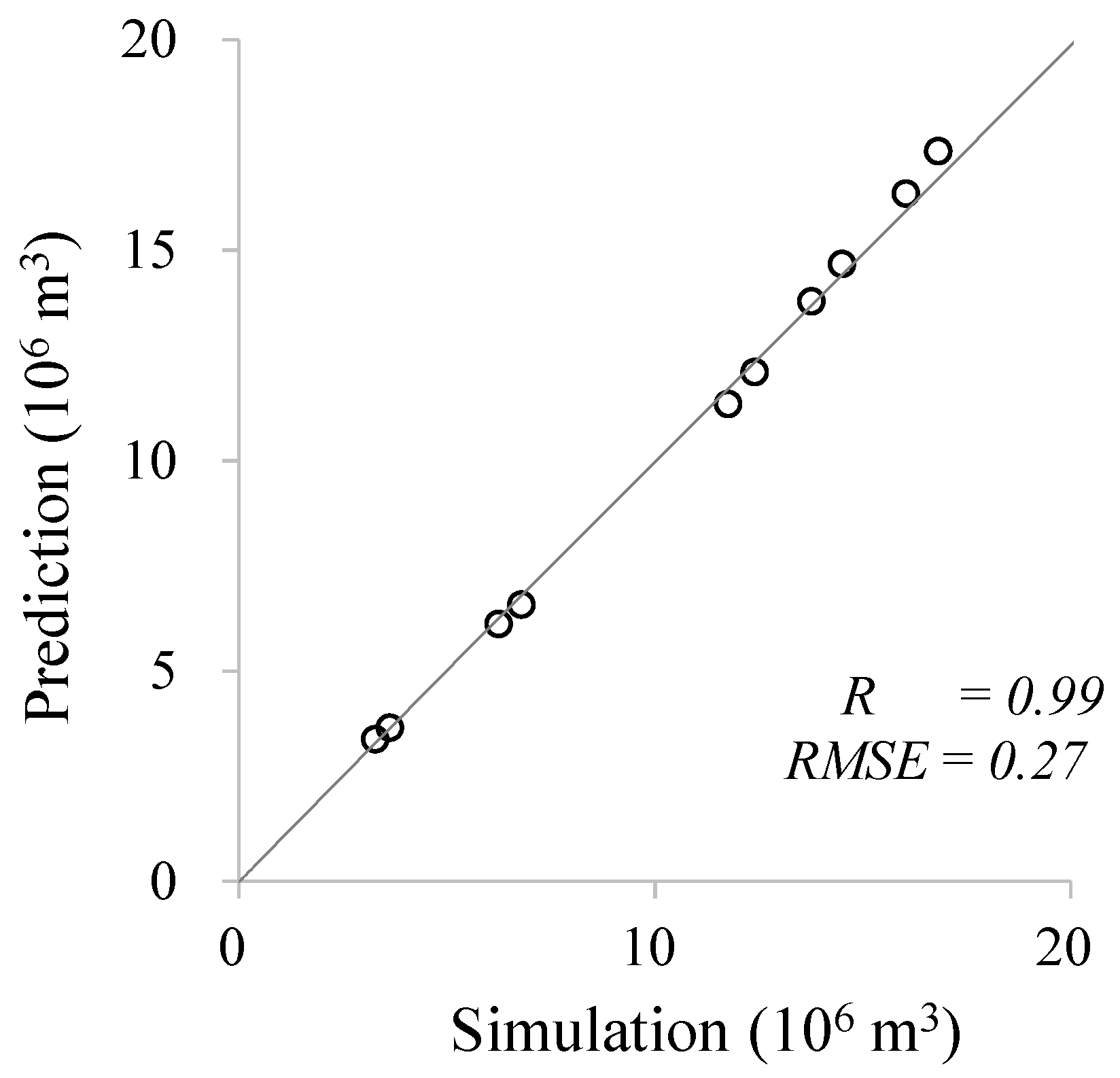
By conducting statistical analysis on the results in Table 12, the relationship between city runoff and watershed runoff can be expressed by the following equation:

$$\frac{V_{watershed}}{V_{city}}={\left(\frac{A_{watershed}}{A_{city}}\right)}^a\times {\left(\frac{IM{P}_{city}}{IM{P}_{watershed}}\right)}^b\times {\left(\frac{R_{city}}{R_{watershed}^{100}}\right)}^c$$

(1)

in which $V_{watershed}$ and $V_{city}$ are runoff volumes on watershed and city scales, respectively; $IM{P}_{watershed}$ and $IM{P}_{city}$ are the area ratios of impermeability on watershed and city scales, respectively; $R_{city}$ is the observed rainfall on city scale; $R_{watershed}^{100}$ is the rainfall on watershed scale under 100-y return period. The coefficients $a,b,c$ are determined by multiple regression analysis which yields $a=3.01,b=0.71,c=0.37$. With correlation coefficient $R=0.99$ and Root-Mean-Square-Error $RMSE=0.27$, the $V_{watershed}$ values simulated by hydrological model are in good agreement with those predicted by the equation, as shown in Figure 10. Being a general expression linking city runoff to watershed runoff, Equation (1) can be applied to any watershed, not only for the specific region in this study. When the ratio of $A_{watershed}/A_{city}$ increases, the watershed will receive more rainfall water and generate more runoff compared with the city. A larger value of $IM{P}_{city}/IM{P}_{watershed}$ represents that impermeable ratio at city increases compared with that at watershed; thus, the city will make a larger contribution to watershed runoff. The ratio of $R_{city}/R_{watershed}^{100}$ allows us to predict watershed runoff from the rainfall observation at city; meanwhile, it reflects the phenomenon that the contribution of city runoff decreases at high discharges. The influence of land use will be implicitly included in the coefficients of $a,b,c$ which vary with watershed conditions.

5. Conclusions

Analyzing runoff variations from land-cover and land-use changes caused by urbanization is critical for flood mitigation. However, analysis should not be conducted only on a city scale but also on larger scales because a city is also a part of a wider watershed or river basin. In this study, land and runoff variations resulting from urbanization are analyzed on the basin scale (large), watershed scale (medium), and city scale (small) for the Zhuoshui River Basin, Taiwan. Based on the scale sizes, different data and models are employed for land interpretation and runoff simulation in the past, at present, and in the future (Table 1). Overall, patterns of land-runoff changes due to urbanization are discovered on the basin scale; discrepancies raised from the usage of different land data and hydrological models are evaluated on the watershed scale; and the impacts of LID facilities on flood reduction in response to urbanization are quantified on the city scale. The research findings for the different scales are summarized as follows:

• On the basin scale, the land-cover transfer matrixes are established from the interpretation of multi-period satellite images. The results show that a large area of vegetation land (10,170 hectares) became bare land from 1998 to 2008, accompanied by a significant increase (40%) in built-up area from 1998 to 2003. This suggests that the major Chi-Chi earthquake, occurred in 1999, increased the pace of urbanization in the process of reconstruction and relocation at a speed faster than the recovery of natural land covers. Through hotspot analysis, built-up areas were discovered to be mainly concentrated in the Jushan and Chi-Chi districts in the study river basin, which was the earthquake epicenter. However, this increase in built-up area is less than 1% of the entire river basin area; therefore, it has no influence on the variation of simulated runoff on the basin scale.
• On the watershed scale, the sub-basins containing Jushan District are selected to simulate the runoff variations with respect to land-cover changes from 1998 to 2013 and land-use changes from 2008 to 2030. Again, no significant land-cover and runoff variations were found from 1998 to 2013, but from 2008 to 2030, the increases in CN and IMP caused by land-use changes lead to 5–10% increases in runoff peak under different return periods. However, in the overlay year of 2008 when the land-cover and land-use data are both available, discrepancies in runoff estimations are found because the values of CN and IMP interpreted from land-use data are much larger than those interpreted from land-cover data. Thus, mixed usage of satellite-interpreted land-cover data and manual-investigated land-use data is not recommended for hydrological analysis unless their uncertainties can be quantified on the same basis. In contrast, the concomitant usage of HEC-1 and SWMM shows no contradiction in runoff results if the same land-use data are applied. According to the results by HEC-1 and SWMM, a regressive relationship is derived for predicting watershed runoff from city runoff multiplied by the parameters of area, IMP, and rainfall raised to certain powers. This regression provides a general expression of runoff scaling between different spatial scales. The good agreement between the simulation and prediction demonstrates that the cross-analysis of land/runoff by multiple models is valuable.
• On the city scale, experimental LID facilities are installed on governmental lands in an attempt to reduce the runoff peaks for Jushan District. The results show that the LID facilities effectively reduce the runoff volumes for all return periods, and the runoff peaks at low return periods will be reduced to a level even less than that at present. However, for high return periods, the introduction of LID instead slightly increases the runoff peaks. Although the “side effects” of LID on increasing runoff at high discharges have been previously discovered, they have not been systematically discussed and require follow-up studies for clarification. Statistically, under 2-y return period, the introduction of LID reduces up to 10% of city runoff volumes, which equals to 2% and 0.02% of watershed and basin runoff volumes, respectively. According to these findings, LID approaches are better regarded as local flood mitigation measures in low-discharge conditions.

References

1. Nirupama, N.; Simonovic, S.P. Increase of flood risk due to urbanization: A Canadian example. Nat. Hazards 2007, 40, 25–41. [Google Scholar] [CrossRef]
2. Saghafian, B.; Farazjoo, H.; Bozorgy, B.; Yazdandoost, F. Flood intensification due to changes in land use. Water Resour. Manag. 2008, 22, 1051–1067. [Google Scholar] [CrossRef]
3. Liu, Y.B.; Gebremeskel, S.; De Smedt, F.; Hoffmann, L.; Pfister, L. Predicting storm runoff from different land-use classes using a geographical information system-based distributed model. Hydrol. Process. 2006, 20, 533–548. [Google Scholar] [CrossRef]
4. Shi, P.J.; Yuana, Y.; Zhenga, J.; Wanga, J.A.; Gea, Y.; Qiua, G.Y. The Effect of Land Use/Cover Change on Surface Runoff in Shenzhen Region, China. CATENA 2007, 69, 31–35. [Google Scholar] [CrossRef]
5. Shalaby, A.; Tateishi, R. Remote sensing and GIS for mapping and monitoring land cover and land-use changes in the Northwestern coastal zone of Egypt. Appl. Geogr. 2007, 27, 28–41. [Google Scholar] [CrossRef]
6. Lambin, E.F.; Baulies, X.; Bockstael, N.E. Land-Use and Land-Cover Change Implementation Strategy; IGBP Report No. 48 and IHDP Report No. 10; International Geosphere-Biosphere Programme: Stockholm, Sweden, 2002. [Google Scholar]
7. Engman, E.T.; Gurney, R.J. Remote Sensing in Hydrology; Chapman and Hall: London, UK, 1991. [Google Scholar]
8. Drayton, R.S.; Wilde, B.M.; Harris, J.H.K. Geographic information system approach to distributed modeling. Hydrol. Process. 1992, 6, 361–368. [Google Scholar] [CrossRef]
9. Mattikalli, N.M.; Devereux, B.J.; Richards, K.S. Prediction of river discharge and surface water quality using an integrated geographic information system approach. Int. J. Remote Sens. 1996, 17, 683–701. [Google Scholar] [CrossRef]
10. Chomitz, K.M.; Gray, D.A. Roads, land use, and deforestation: A spatial model applied to Belize. World Bank Econ. Rev. 1996, 10, 487–512. [Google Scholar] [CrossRef]
11. Martínez, J.M.; Suárez-Seoane, S.; De Luis Calabuig, E. Modelling the risk of land cover change from environmental and socio-economic drivers in heterogeneous and changing landscapes: The role of uncertainty. Landsc. Urban Plan. 2011, 101, 108–119. [Google Scholar] [CrossRef]
12. Xian, G.; Crane, M.; Su, J. An analysis of urban development and its environmental impact on the Tampa Bay Watershed. J. Environ. Manag. 2007, 85, 965–976. [Google Scholar] [CrossRef] [PubMed]
13. Morita, H.; Hoshino, S.; Kagatsume, M.; Mizuno, K. An Application of the Land-Use Change Model for the Japan Case Study Area; IIASA Interim Report IR-97-065; International Institute for Applied Systems Analysis: Laxenburg, Austria, 1997. [Google Scholar]
14. Serra, P.; Pons, X.; Saurí, D. Land-cover and land-use change in a Mediterranean landscape: A spatial analysis of driving forces integrating biophysical and human factors. Appl. Geogr. 2008, 28, 189–209. [Google Scholar] [CrossRef]
15. United States Army Corps of Engineers (USACE). Hydrologic Modeling System: HEC-HMS Technical Reference Manual; Hydrologic Engineering Center: Davis, CA, USA, 2000.
16. Nageshwar, R.B.; Wesley, P.J.; Ravikumar, S.D. Hydrologic parameter estimation using geographic information systems. J. Water Res. Plan. Manag. 1992, 11, 492–512. [Google Scholar]
17. Schumann, A.H. Development of conceptual semi-distributed hydrological models and estimation of their parameters with the aid of GIS. Hydrol. Sci. J. 1993, 38, 519–528. [Google Scholar] [CrossRef]
18. Xu, Z.; Zhao, G. Impact of urbanization on rainfall-runoff processes: Case study in the Liangshui River Basin in Beijing, China. Proc. Int. Assoc. Hydrol. Sci. 2016, 373, 7–12. [Google Scholar] [CrossRef]
19. Guo, F.; Hanfei, Q.U.; Zeng, H.; Cong, P.; Geng, X. Flood hazard forecast of Pajiang River flood storage and detention basin based on MIKE21. J. Nat. Disasters 2013, 22, 144–152. [Google Scholar]
20. U.S. Environmental Protection Agency (USEPA). Storm Water Management Model User’s Manual Version 5.1; National Risk Management Laboratory Office of Research and Development: Cincinnati, OH, USA, 2015.
21. Guan, M.; Sillanpää, N.; Koivusalo, H. Modelling and assessment of hydrological changes in a developing urban catchment. Hydrol. Process. 2015, 29, 2880–2894. [Google Scholar] [CrossRef]
22. U.S. Environmental Protection Agency (US EPA). Low-Impact Development Design Strategies: An Integrated Design Approach; EPA 841-B-00003; US EPA: Washington, DC, USA, 1999.
23. British Columbia Ministry of Environment (BCME). Stormwater Planning: A Guidebook for British Columbia; Government of British Columbia: Victoria, UK. Available online: http://www.toolkit.bc.ca/resource/stormwater-planning-guidebook-british-columbia (accessed on 24 January 2018).
24. Olewiler, N. The Value of Natural Capital in Settled Areas of Canada; Ducks Unlimited Canada and The Nature Conservancy of Canada: Toronto, ON, Canada, 2004. [Google Scholar]
25. Sharma, A.K.; Pezzaniti, D.; Myers, B.; Cook, S.; Tjandraatmadja, G.; Chacko, P.; Chavoshi, S.; Kemp, D.; Leonard, R.; Koth, B. Water sensitive urban design: An investigation of current systems, implementation drivers, community perceptions and potential to supplement urban water services. Water 2016, 8, 272. [Google Scholar] [CrossRef]
26. U.S. Environmental Protection Agency (USEPA). Combined Sewer Overflow (CSO) Control Policy; Federal Register; United States Environmental Protection Agency: Washington, DC, USA, 1994; Volume 75, pp. 18688–18698.
27. Ministry of Housing and Urban-Rural Development (MHURD). Technical Guide for Sponge Cities—Water System Construction of Low Impact Development; Ministry of Housing and Urban-Rural Development: Beijing, China, 2016.
28. Li, H.; Ding, L.; Ren, M.; Li, C.; Wang, H. Sponge city construction in China: A survey of the challenges and opportunities. Water 2017, 9, 594. [Google Scholar] [CrossRef]
29. McCutcheon, M.; Wride, D.; Reinicke, J. An evaluation of modeling green infrastructure using LID controls. J. Water Manag. Model. 2012, 193–205. [Google Scholar] [CrossRef]
30. Chen, B.; Liu, J.; She, N.; Xu, K. Optimization of low impact development facilities in Beijing CITIC complex. In Proceedings of the International Low Impact Development Conference, Houston, TX, USA, 19–21 January 2015; pp. 342–351. [Google Scholar]
31. Lucas, W.C.; Sample, D.J. Reducing combined sewer overflows by using outlet controls for Green Stormwater Infrastructure: Case study in Richmond, Virginia. J. Hydrol. 2015, 520, 473–488. [Google Scholar] [CrossRef]
32. Guo, C.Y. Detention basin sizing for small urban catchments. J. Water Resour. Plan. Manag. 2012, 125, 1–5. [Google Scholar]
33. Jayasooriya, V.M.; Ng, A.W.M. Tools for modeling of stormwater management and economics of green infrastructure practices: A review. Water Air Soil Pollut. 2014, 225, 2055–2061. [Google Scholar] [CrossRef]
34. Peng, H.Q.; Liu, Y.; Wang, H.W.; Ma, L.M. Assessment of the service performance of drainage system and transformation of pipeline network based on urban combined sewer system model. Environ. Sci. Pollut. Res. 2015, 22, 15712–15721. [Google Scholar] [CrossRef] [PubMed]
35. Tao, J.; Li, Z.; Peng, X.; Ying, G. Quantitative analysis of impact of green stormwater infrastructures on combined sewer overflow control and urban flooding control. Front. Environ. Sci. Eng. 2017, 11, 11. [Google Scholar] [CrossRef]
36. Nantou County. Revision of Urban Planning Project for Jushan Township; Nantou County: Nantou City, Taiwan, 2013. (In Chinese) [Google Scholar]
37. Vapnik, V.N. The Nature of Statistical Learning Theory; Springer: New York, NY, USA, 1995. [Google Scholar]
38. Selçuk, R. Analyzing land use/land cover changes using remote sensing and GIS in Rize, North-East Turkey. Sensors 2008, 8, 6188–6202. [Google Scholar]
39. Cliff, A.C.; Ord, J.K. Spatial Autocorrelation; Pion Limited: London, UK, 1973. [Google Scholar]
40. Ord, J.K.; Getis, A. Local spatial autocorrelation statistics: Distributional issues and an application. Geogr. Anal. 1995, 27, 286–306. [Google Scholar] [CrossRef]
41. Moran, P.A.P. Notes on continuous stochastic phenomena. Biometrika 1950, 37, 17–23. [Google Scholar] [CrossRef] [PubMed]
42. Getis, A.; Ord, J.K. The analysis of spatial association by use of distance statistics. Geogr. Anal. 1992, 24, 189–206. [Google Scholar] [CrossRef]
43. Singh, V.P. Applied Modeling in Catchment Hydrology; Water Resources Publications: Littleton, CO, USA, 1982. [Google Scholar]
44. U.S. Department of Agriculture (USDA). Urban Hydrology for Small Watersheds; Technical Release 55 (TR-55); Natural Resources Conservation Service, Conservation Engineering Division: Washington, DC, USA, 1986.
45. National Land Survey and Mapping Center (NLSC). The Second National Land-Use Survey; Ministry of Interior: Taipei, Taiwan, 2008.
46. Horner, W.W.; Flynt, F.L. Relation between rainfall and run-off from small urban areas. Proc. Am. Soc. Civ. Eng. 1936, 101, 140–183. [Google Scholar]
47. Water Resource Agency (WRA). Handbook for Hydrological Design; Water Resource Agency: Taichung, Taiwan, 2001. (In Chinese)
48. Nantou County. Review and Planning for Jushan Township Sewer System; Nantou County: Nantou City, Taiwan, 2008. (In Chinese) [Google Scholar]
Figure 1. Study areas on different scales.
Water 10 00106 g001
Figure 2. Hotspots of artificial structures on basin scalein (a) 1998; (b) 2003; (c) 2008; (d) 2013.
Water 10 00106 g002aWater 10 00106 g002b
Figure 3. Present and future land-use maps on watershed scale: (a) present; (b) future.
Water 10 00106 g003aWater 10 00106 g003b
Figure 4. Present and future runoff peaks on watershed scale for (a) W19 and (b) W20.
Water 10 00106 g004
Figure 5. Runoff hydrographs under 2-y return period for watersheds (a) W19 and (b) W20.
Water 10 00106 g005
Figure 6. Drainage divisions on city scale.
Water 10 00106 g006
Figure 7. Present and future land-uses on city scale: (a) present; (b) future.
Water 10 00106 g007
Figure 8. Comparison between present and future IMP on city scale.
Water 10 00106 g008
Figure 9. (a) Runoff peak and (b) runoff volume for different return periods under land-use scenarios of present, future, and future with LID.
Water 10 00106 g009
Figure 10. Comparison between the simulated and predicted runoff volumes on watershed scale.
Water 10 00106 g010