A Numerical Approach to Predict Water Levels in Ungauged Regions—Case Study of the Meghna River Estuary, Bangladesh


1
Department of Civil and Environmental Engineering, Incheon National University, Incheon 22012, Korea
2
International Center for Urban Water Hydroinformatics Research & Innovation, Incheon 21999, Korea
*
Author to whom correspondence should be addressed.
Water 2018, 10(2), 110; https://doi.org/10.3390/w10020110
Submission received: 26 October 2017
/
Revised: 17 January 2018
/
Accepted: 17 January 2018
/
Published: 27 January 2018
Abstract
:Quantitative flood frequency investigation in a large estuary is somewhat challenging by numerical modelling, because the model optimization depends on the appropriate physical and hydrodynamic properties of the estuarine river. This study attempts to solve the bathymetry configurations of the Meghna River estuary and the assimilation of flow data, which exposed an important role in water level prediction. Upstream flow rates and nonlinear semidiurnal tides have an impact on the instability of the flow in this estuarine river. A large amount of flow accumulates in the upstream confluence against or in favor of tides during the rainy season from the adjacent river basins and significantly moves in the Bay of Bengal. The aim of this study is to predict water levels in the un-gauged regions of the Meghna River estuary. A numerical technique was developed using Mike21 flexible mesh, comprising shallow water hydrodynamic components in the estuary. Subsequently, log-normal distribution was employed to analyze the flood magnitudes among the ungauged stations of the estuary. The calibration results comprised with the observed water levels adequately. In conclusion, these water level prediction results can be applied to alleviate the coastal land from extreme flooding and to design hydraulic structures in the narrow streams.
1. Introduction
Climate change is the biggest environmental threat faced by South Asian countries [1,2]. This problem will be even worse in the coming decades. While the developed world has awakened to the threat of climate change, the true enormity of how this could eventually affect to the developing world still does not concern their governments. A recent report showed that about 125 million migrants from Bangladesh and India could be rendered homeless by the end of this century [3]. It is well established that current direction and speed have a direct influence on river erosion and deposition, ship navigation, tidal power plants and fish migration.
The river networks of Bangladesh form an extensive flow path (approximately. 24,000 km) which covers about 7% of the total surface area of the country. Both the river discharge and tides have an impact on the instability of the river flow in coastal basins. Accordingly, it is essential that areas near coastal watersheds make the necessary preparations against potential floods caused by upstream river discharge and tides. The coastal zone has great economic and ecological value as it supports extensive agricultural activities, large forestry and plentiful aquatic life. Two factors that can have the greatest impact in the region are the rise in sea level and storm surges where 30% of the agricultural land is located in the coastal region [4,5]. Taormina et al. tried forecasting river flow by ANN and swarm optimization [6]. Chau et al. and Wu et al. have given a solution for rainfall prediction by machine learning techniques [7,8]. Chen et al. and Wang et al. provided methodologies for river flow estimation [9,10]. The prediction methods are important and generally possible to apply with time series data collected for years. However, there are many data sparse regions which need models for data collection. In this study, we tried to develop a model for the prediction of flow characteristics with limited data and the prediction models recently suggested above can be applied for future study with collected data based upon this study.
In addition, there are several previous studies for the investigation and prediction of hydrodynamic characteristics in the data sparse regions in Asian countries. Ahmed (2004) indicated that multipurpose river basin development (MRD) is a necessary approach for disaster management, basin-wide development, ecosystem protection and regional institutional framework [11]. Mirza (2011b) states that variations in flood extent and depth are the result of changes in peak discharges in the Ganges, Brahmaputra and the Meghna Rivers [12]. These problems lead to instability in water levels and severe floods and river erosion in this region. Dasgupta et al. (2009b) state that more than 30% of the cultivable land in Bangladesh is in the coastal area and 1m sea level rise could affect around 23% of Bangladesh’s total coastal land area [13]. Most of the coastal regions of Barisal, Patuakhali, Sundarbans, Bhola, Hatia and Sandwip wouls be inundated by saline or brackish water, creating serious saline waterlogging problems. Salt-water intrusion along the Meghna River estuary may reach up to the Mymensingh and Sylhet districts upstream. The surface water salinity of the Karnaphuli and Matamuhuri network in the greater Chittagong district may also be affected. The land use practices in watersheds during the last few decades will have a potential impact on this study area: (i) amount of runoff that results from rainfall in a watershed, (ii) water-carrying capacity of a drainage basin, and (iii) change in land elevations with respect to the riverbeds and sea level [14]. In Bangladesh, riverbank erosion and the deposition of sediments are a regular phenomenon which creates enormous problems for the socio-economic and environmental sector [15]. The morphological changes may occur due to the hydrodynamic forces of wave action, tidal effect and river discharge. The banks of the lower Meghna near Chandpur have been eroded continuously and information on the river bank lines for the last 73 years shows progressive recession of the left bank [16]. In a cyclone study it was illustrated that storm surges originate in the central and southern parts of the Bay of Bengal due to the shallow continental shelf and the surge amplifies to the low-lying, poorly-protected coastal areas [17].
In this study, the Mehgna River estuary is adopted as the case study. There are several alternative study areas for this study, however, we selected the Meghna River estuary in consideration of the importance of region, as there are several issues around the region and it is a typical data sparse region with limited data available.
Meghna has an estuary which is one of the largest estuaries on the earth in terms of sediment–water discharge located at the central part of the coastline. The area is characterised by high levels of hydro-dynamic activity. Erosion and deposition occur concurrently and the rates of both are high. The area is periodically subject to severe storms and cyclones. The sediment discharge from the Meghna River is the highest and the water discharge is the third highest among all the river confluences in the world. Due to the high sediment discharge, lands are eroded and reformed. The water flow patterns also shift [18] in the Meghna River estuary.
The lower Meghna River carries a combined flow of water typically 120,000 m3/s, except for extreme flood events. About 85% of the water flow comes from the Ganga, Jamuna and Padma River confluence from the North-West regions, whereas the remaining 15% comes from the upper Meghna River and the North-Eeast regions of Bangaldesh. Along the Meghna River estuary, there are a number of deltaic islands which create the highly dynamic and morphologic features in distinct seasons. The river basin sites are generally submerged due to the continuous rainfall for a short duration (i.e., a week) of time but the water is drained away slowly by semidiurnal tides (max. 1.4 m) occurring twice in a day at the downstream area of Chandpur and the Bay of Bengal [19].
The regions surrounding the Meghna River estuary of Bangladesh are suffering from severe floods with effects on the river flow, tides and monsoon climate. Moreover, Bangladesh has insufficient instantaneous river gauge observed data or systems to warn of the risk of such disasters. The purpose of this study is to investigate real time estuarine river flow based on hydrodynamic modelling to predict ungauged station flood water levels. This study concludes the comprehensive description of the estuarine river modelling schemes in terms of numerical analysis and solution methods. Therefore, in addition to numerical and statistical frequency analysis, a validation of the hydrodynamic model predictions was illustrated.
This study was carried out to implement a hydrodynamic model based on the prediction of water levels and through the real-time 15-min interval data in the Meghna river estuary using limited gauging stations. Although the daily maximum and minimum water level and discharge data are known at the upstream river gauge station, the downstream sea tide measurement was 15-min interval data. Short duration/real-time data was the main obstacle to implementing this model. Besides, this model domain requires boundary condition data with similar time steps, which interpolated and predicted hydro-dynamically with the physical processes (domain, mesh, bathymetry, and riverbed resistance).
1.1. Physical Settings of Estuary
In this study, a total 24,205 km2 domain was considered for the hydrodynamic modelling of the lower Meghna River estuary. The geophysical extent of the study area was mapped on the BTM (Bangladesh Transverse Mercator) Cartesian coordinates extending from 750,000 m (North) to 345,000 m (South) and 740,000 m (East) to 400,000 m (West). The extent of the modelled estuarine watercourse is about 7825 km2 within the lower Meghna, Buriswar, Tentuli, Sibsa and Pasur River. The maritime extent was 4776.4 nautical miles (16,382.6 km2) with a depth array from 0 to −9 m from the coast to the open sea boundary. The combined flow of the Ganges and Brahmaputra (Jamuna) River carried by the Padma River, which further meets with a wide (11 km) confluence at the Meghna River during the monsoon near Chandpur. The river mouth shifted from the East to the West side of the Hatia and Monpura islands. The length between upstream and the coastal confluence of the lower Meghna River main channel is about 110 km and 150 km, respectively. The Meghna River estuary is one of the widest coastal estuarine rivers in the world. The width of the main channel varies from 2.5 km to 22.4 km with the above 100 m width of major linked rivers. Another extensive river named Tentulia lies directly between the open sea and 30 km south of the upstream boundary. Therefore, the routing buffer zones of the lower Meghna River estuary have 22,156 km2 coastal towns where the semidiurnal tide directly governs stream and estuarine flows.
1.2. Hydrological Settings
The hydrological setting of the study area has an annual rainfall of 3000~4900 mm in upstream regions and 1500~2400 mm in downstream regions (Chandpur). Generally, during June to August the upstream region experiences (52%) rainfall (1600 mm~2500 mm) and the downstream region experiences (60%) rainfall (900 mm to 1500 mm). Consequently, the upper Meghna River basin flow accumulates from the upstream region at Bhairab station, which later meets with the Dhaleswari River and discharges downstream at Chandpur station. However, the downstream (Chandpur) station is at a river confluence where 15% river flow comes from the upper Meghna River (North East region) and rest of the 85% flow comes from the Jamuna, Ganga and Padma Rivers (North West region). In this estuarine region, a huge amount of discharge and tidal fluctuation creates numerous flooding problems (i.e., extensive submerging, river channel instability, repetitive erosion of cultivated lands, the settlement and displacement of people).
Data assimilation has been found to be problematic for the hydraulic modeler when developing a calibrated estuarine river model. The scope of this study is hydrodynamic model optimization with numerical schemes. Below is the study of the hydrodynamics of the Meghna River estuary the coastal region of Bangladesh. The lower Meghna River estuary houses an upstream river gauge station (Chandpur), while the lower Meghna River estuary and coastal region was considered the computational domain to predict the un-gauged stations’ tidal water level and to investigate the hydrodynamic phenomena. The lower Meghna estuary and coastal region serve as the prime fishing locations in Bangladesh; these sufficiently fulfill national fishing demands and stimulate the local economy with the exportation of the fish. Rising water levels cause lateral flows within the undefined river banks that create flooding and waterlogging issues, whereas low water levels create navigation problems. Figure 1 shows the detailed view of the study area of the lower Meghna River estuaries and their adjacent watershed boundaries, the locations of the tidal river gauge stations (green symbols), and the locations of the un-gauged station water level predictions (black triangle symbols).
2. Materials and Methods
2.1. Hydrodynamic Model
The estuarine river two-dimensional model was used to predict water hydro-dynamically because it used numerical techniques to solve the vertically integrated governing equations adequately [20,21]. Although the latest technology for the numerical study of estuary hydrodynamic modeling is applying a three-dimensional model, we adopted a two-dimensional model since most of the analyses of the estimation of the river’s properties suffer from a lack of real time measurements, a shortage of the duration of measurements, and limited gauging locations for water and river bed levels, moreover it was only possible to establish the bathymetry of the model domain with limited resolution data. The hydrodynamic model involves the spatial discretization of the study domain and the governing equations using either the finite difference or finite element method and the integration of the resulting equations over time using a suitable time stepping procedure. The numerical models based on these equations, which include non-linear interactions, is a most powerful method for the practical prediction of surges, especially for domains with complex bathymetry and coastline configurations. The accuracy of the simulation of storm surges using numerical models depends on various input or calibration parameters such as storm characteristics, bathymetry, tides and the representation of the estuarine river geometry. Therefore, these models require proper boundary condition data for water levels and discharge to perform hydrodynamic simulations [22].
The hydrodynamic model is based on the numerical solutions of two-dimensional, depth-integrated (incompressible Reynolds-averaged) Navier–Stokes equations along with the governing equations for shallow water and transport, and mass and momentum equations. In this study, the MIKE 21 flexible mesh hydrodynamic module (MIKE 21 FM HD) was adopted as the main modeling tool. The MIKE 21 model is a well-known tool which solves the equations of continuity and conservation of momentum using implicit finite different methods. We chose this model because of advantages such as: (i) the multiple values of surface elevation are account simultaneously; (ii) it implicates the measurement of still water depth, total depth, velocity, current speed, flow directions, discharge flux and the Courant Friedrich-Levy (CFL) number, etc.; (iii) allowing the spatial and temporal water distribution for the whole domain; (iv) the capability to calibrate the simulated flow within the gauged and ungauged stations; (v) consistency to model the river hydraulics accurately through the adequate mesh densities; (vi) high visual output and easy interpretation; (vii) assess the multi-purpose engineering problems, for example: river bank flooding and erosion, levee removal, dam break, sediment transport and mobile bed, bank erosion protection design and analysis, river restoration or dredging design, hydroelectric or barrage and mitigation projects. This means that although the study area is a typical data sparse region, it is possible to apply the numerical model used in several further research projects.
The MIKE 21 flexible mesh (FM) hydrodynamic (HD) model numerical engine uses the implicit finite difference technique to solve these governing equations for a given boundary condition on a staggered two-dimension grid. The numerical scheme called alternating direction implicit (ADI) and provides stable results under reasonable computational costs and accuracy. The applicability of the ADI on hydrodynamic modelling has also been proven by earlier studies [23,24]. The mass transport equations of hydrodynamic models (Mendelsohn and Swanson, 1991), which were later applied to solve the boundary-conforming, transformed grid using the well-known finite difference solution technique [25,26]. An approximation of the Riemann solver employed for the computation of convective fluxes makes it possible to handle discontinuous solutions. It involves an explicit scheme of time integration. Subsequently, the Courant Friedrich-Levy (CFL) number less or equal to one is the numerical stability criterion of this model. This module can simulate unsteady or nonlinear two-dimensional (2D) flows in a vertically (depth-averaged) homogeneous layer (one layer) of fluids and has been applied in a large number of studies around the world [27].
2.2. Meghna Estuarine River Modelling (Methodology)
In this study, the numerical modelling was conducted generating a MIKE 21 FM HD model for the Meghna River estuary. Cartesian coordinates are used to model the study domain. The domain’s horizontal plane as well as the spatial extent were isolated with non-overlapping triangular or quadrilateral elements besides mesh. This model is used to predict the water levels in un-gauged regions. Earlier studies have stated that it is an effective tool in numerical modelling for the prediction (or simulation) of water levels and the flow of estuaries, bays, coastal regions, flood plains and rivers [17]. Consequently, model simulations include several phenomena of hydrodynamics, e.g., water levels, velocities, current speeds and directions, and pressure and discharge fluxes in response to versatile forcing functions.
2.2.1. Modeling and Calibration
The riverbed resistances of Manning and Chezy numbers were specified considering the variable depth for calibrating the MIKE 21 FM HD model. The drag coefficient (0.002) within the particle size 0.1 ± 0.03 mm was used to measure bed resistances [28,29,30]. Moreover, the initial values were specified for eddy viscosity (0.2) and CFL number (0.8), respectively. The CFL number is accounted in the MIKE 21 FM HD module for the numerical stability criterion. The model calibration process was conducted using two distinct seasons (dry and rainy).
2.2.2. Analytic Prediction of Water Levels
In this study, the accuracy of the MIKE 21 FM HD models simulation is compared with the observed data through the stepwise simple linear regression model. A detailed description of stepwise regression models are discussed and verified [31]. The statistical model was employed to obtain R2, mean standard error (MSE) and mean absolute percentage error (MAPE). Besides regression, a log-normal distribution (LN3) of the frequency analysis was conducted to determine the flood water level return periods in the un-gauged regions of the Meghna river estuary.
2.3. Computational Domain
There is a growing need to achieve accurate mesh and bathymetry data for estuarine river models [32,33]. Mostly, the river bathymetry data are collected from the cross-sections or discrete points. In the literature, several studies stated that topographic data, mesh resolution, and bed roughness significantly affect the shallow water flow [34,35,36]. Therefore, the roughness was needed to specify either constant or spatially variance in the domain or in the corresponding mesh configurations [37]. This study proceeds with the Chezy and Manning variable regarding the spatially varied river depth and the averaged bed resistance (roughness) domains corresponding to the mesh configuration. In the case of the hydrodynamic modeling of the estuarine river, the triangular irregular network (TIN) process was required for mesh generating. TIN mesh conserves critical elevation data such as topography, river bed elevation and boundary. Prior to constructing a mesh or bathymetry the TIN interpolation was applied using the MIKE Zero mesh generator for this study domain. Previous studies found this interpolation technique to be an adequate method to construct a domain/bathymetry [38]. Moreover, the scatter data was used from the digital elevation model (DEM) for triangulations which provide flexibility in the boundaries of a computational domain [39].
The computational domain of this study was constructed on Bangladesh Transverse Mercator (BTM) Cartesian coordinates using 1000% (size of bounding) beyond the convex hull of the scatter data. Several researchers directly used the topography to build the mesh or grid to develop a numerical simulation with a huge number of elements that may need a large amount of computational time and space [40]. In this study, the scatter-grid data of the lower Meghna River estuary was considered with 10 m threshold depth due to the limited computer computation facility. The grid size of the triangular element varied from approximately 30 m around the internal islands, rivers and maximum 380 m for estuaries or the open sea. To reduce the computation time, for a large area a fine resolution mesh takes more space and a computer has the limitation to compute and create the mesh. The mesh of this domain specified 2,460,177 scatter elevation points that required approximately 130.1 h (5.4 days) computing time for a three-month simulation (15 min intervals). The boundaries, mesh and bathymetry of the Meghna River estuary subtracted for the computational domain is shown in Figure 2.
2.4. Water Level and Inflow Boundary Conditions
The initial and boundary conditions are an important factor for implementing the MIKE 21 FM HD model as well as for numerical solutions. In the case of estuarine river models, the hydrodynamic, morphologic, and oceanography predictions are based on the solutions of fundamental partial differential equations and the assimilation of measurement data [41,42]. Both the initial and boundary conditions are essential for computations of hydrodynamic models. However, the accuracy of the model simulations depends on the partial differential equations because of the time-dependent boundary conditions. The boundary conditions can frequently be collected at gauge stations from different locations of the river [43]. In case of large rivers, the boundary conditions are difficult know at the boundaries of the computational domain because of the limitations of obtaining observed data from sufficient gauge stations. The time and amplitude of the tides at a location influence the pattern of tides in the deep ocean, the amphidromic systems of the oceans, and the shape of the coastline and near-shore bathymetry [44].
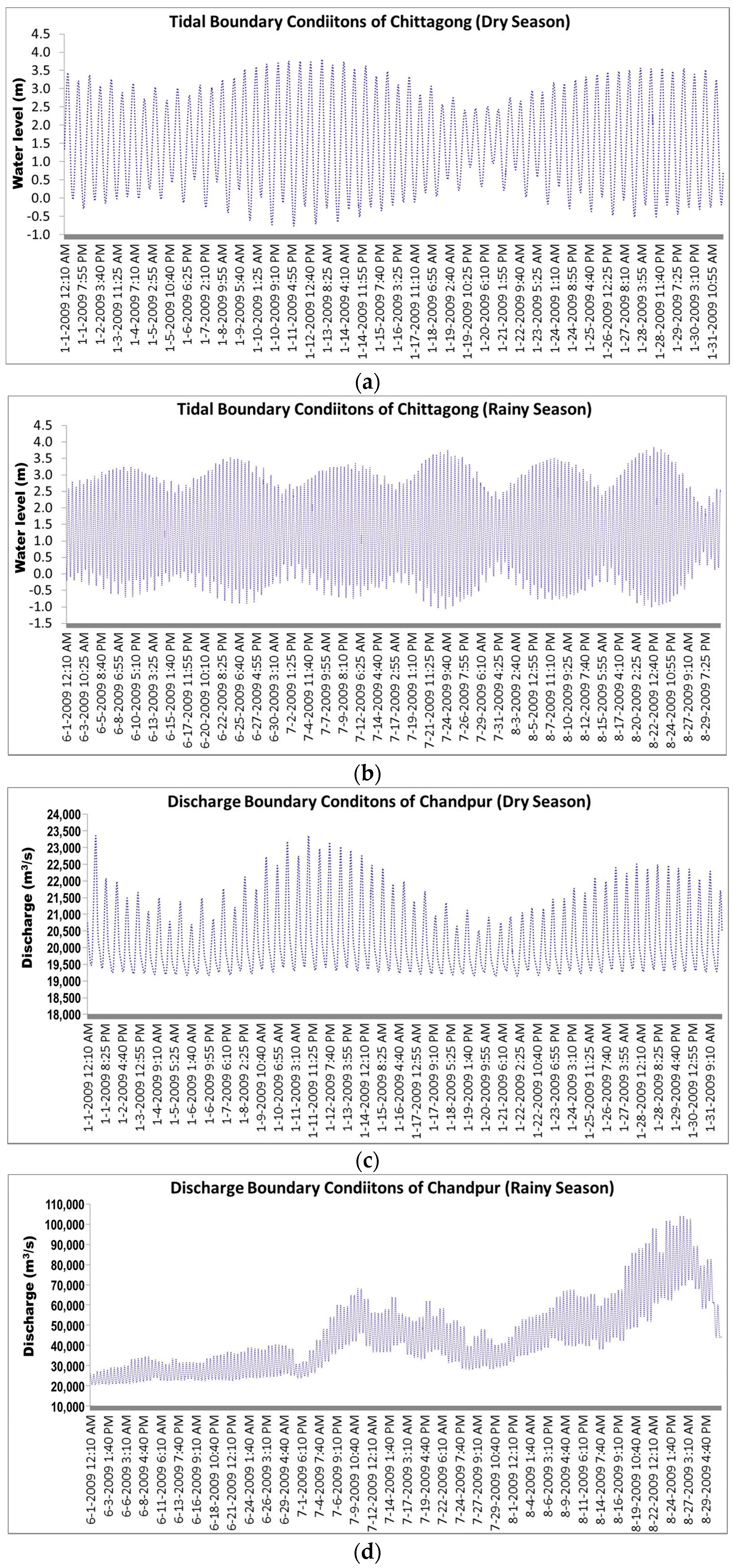
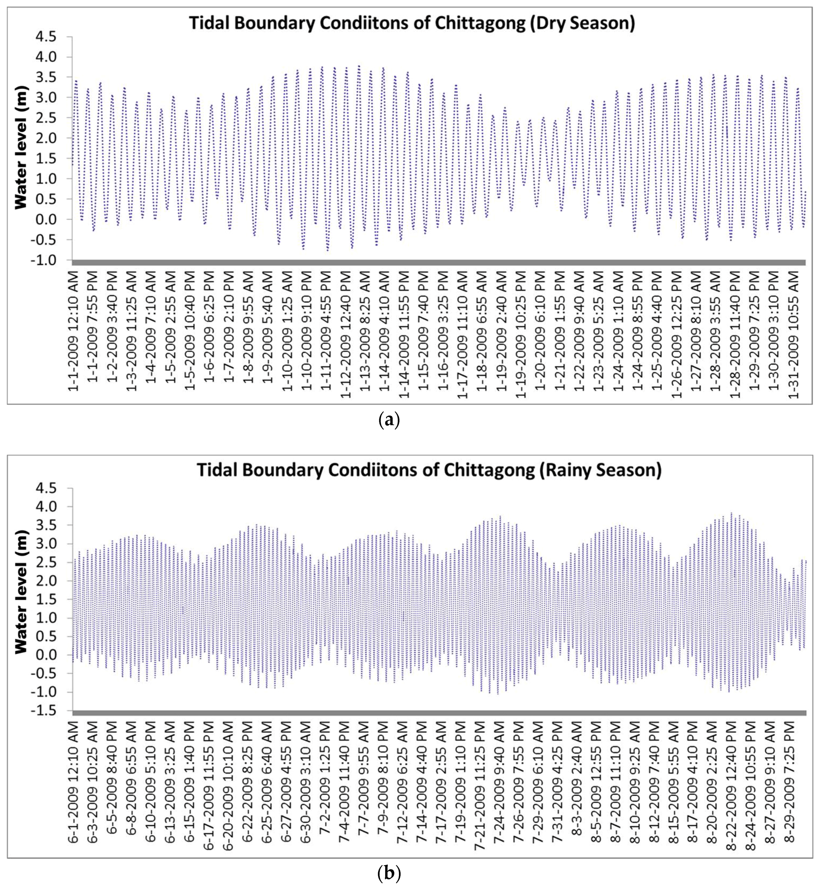
The cubic spline is a time series interpolation technique which fits a polynomial curve to a set of data points. Several researchers have documented and prescribed cubic spline curve fit techniques to obtain a smooth curve through data points [45,46]. The cubic spline is one type of a French curve or an architect’s spline and is subjected to smoothing curve fit interpolation techniques. Natural hydrographs of water levels and discharge values (daily max and min) were obtained from the Bangladesh Water Development Board’s (BWDB) real upstream gauge station at Chandpur. The cubic spline interpolation method was employed to regenerate the discharge pattern and to obtain the discharge boundary conditions in shorter time steps (15 min). The observed daily maximum and minimum discharge values of the upstream river gauge station (Chandpur) were interpolated using cubic spline and applied as a boundary condition to calibrate the hydrodynamic model [47,48]. Therefore, the sea tidal water level (15-min) pressure gauge measured data was collected from the Chittagong port station and applied as amphidromic (open sea) boundary conditions for this computational model. The simulation periods were conducted in the dry season for one month (1 to 31 January 2009) and in the rainy season for three months (1 June to 31 August 2009). Both the rainy and dry season boundary conditions were applied in the hydrodynamic model of the Meghna river estuary and are presented in Figure 3.
3. Results
3.1. Model Calibration
The hydrodynamic model was calibrated using the variable Manning and Chezy riverbed resistances for both the dry and rainy seasons. Most of the riverbeds are recognized as ripple sand types of materials. Linear regression analysis, with a 95% confidence interval, showed good agreement in both seasons between the observed and predicted (MIKE 21 FM HD) water level in the upstream boundary during calibration. As the observed water levels from the BWDB were available at the upstream boundary, with daily maximum and minimum values, therefore the simulated water levels were extracted with the communal time of the BWDB observations. Significant calibration results were obtained comparing these water levels. Subsequently, the water level prediction of ungauged regions and the synthesis of major hydrodynamic components in the temporal and spatial extent comprised the optimum calibration.
3.1.1. Calibration for Dry Season (January)
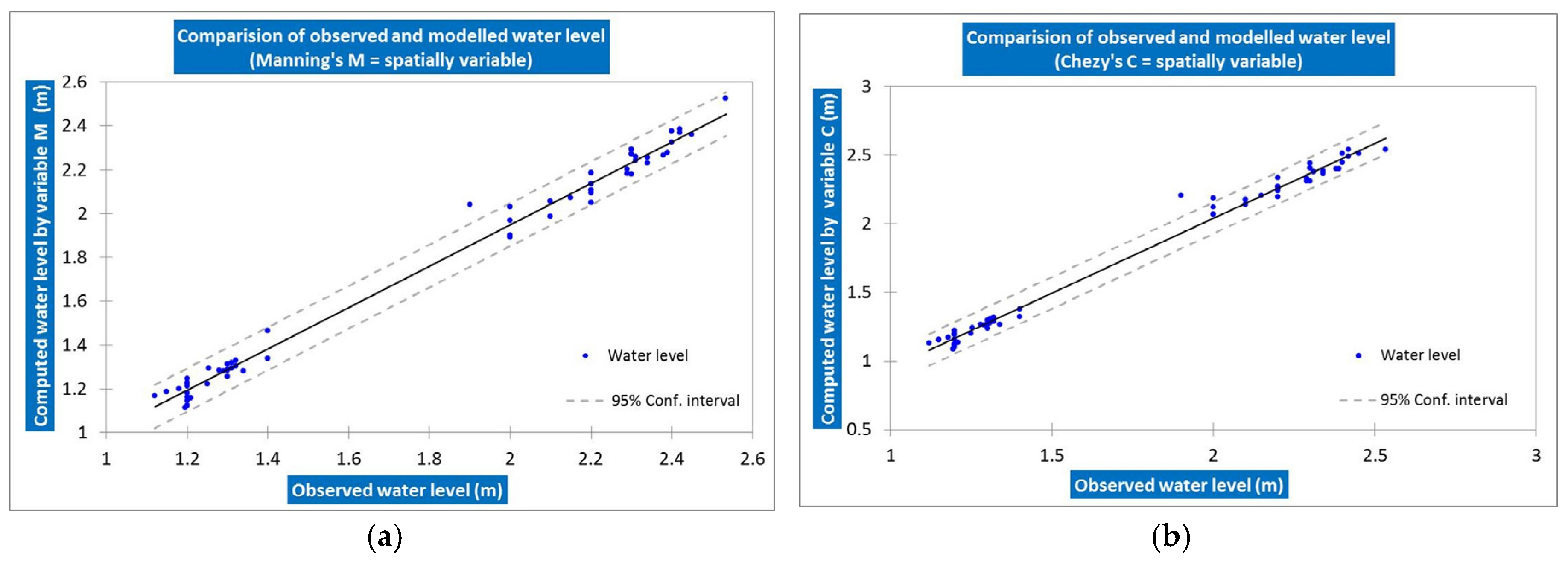
The regression model was separately employed for the Manning variable and Chezy variable corresponding to 62 observations in the dry season. The daily maximum and minimum values (water level) at the upstream river gauge station is compared where the x axis indicates observed data (BWDB data) and the y-axis indicates the hydrodynamic model’s predicted water levels (Figure 4). In the case of the Chandpur river gauge station, evaluation of the regression model indicates correlation coefficients of 0.988 for Manning and of 0.997 for Chezy. Specifically, the mean standard error (MSE) was 0.003 m and 0.001 m for Manning and Chezy bed resistance, respectively, and the mean absolute percent error (MAPE) was 2.216% and 2.014% for Manning and Chezy bed resistance, respectively. Therefore, the calibration precision of the hydrodynamic model is presented in Table 1 for the dry season.
3.1.2. Calibration for Rainy Season (June to August)
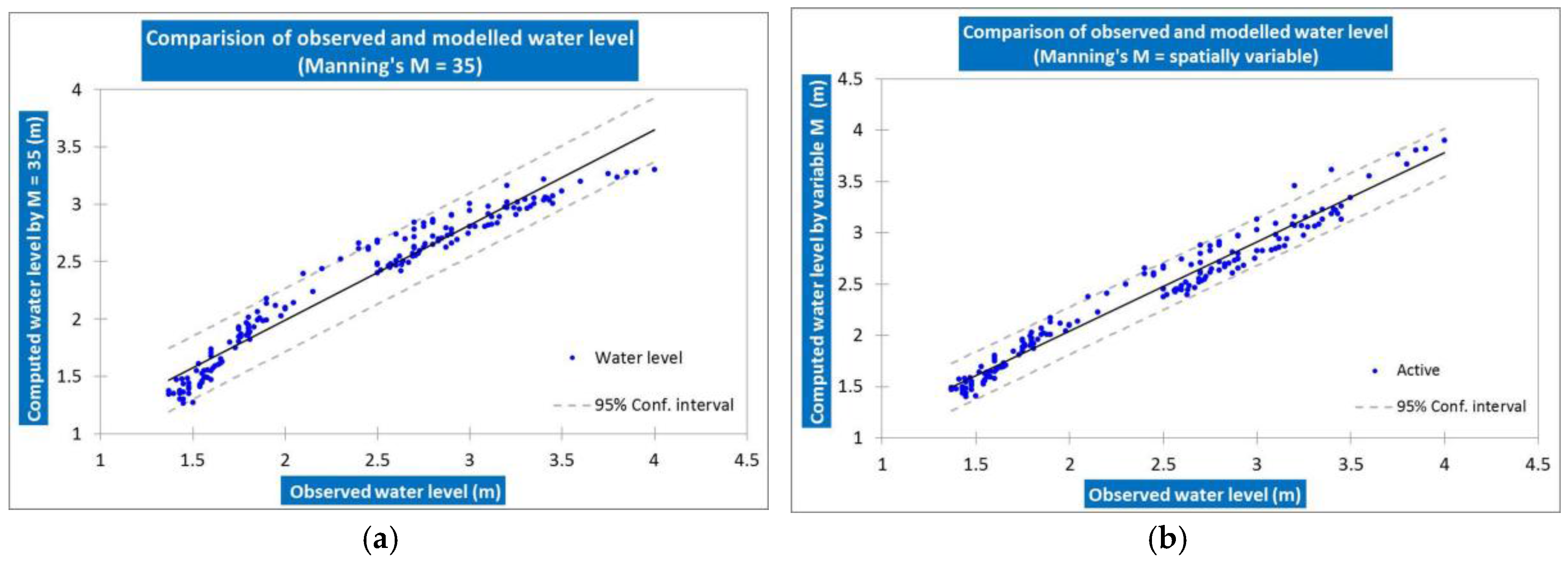
To calibrate the model accuracy for the rainy season, the four (4) cases were considered, for instance constant Manning as 1/n = 35 and constant Chezy as C = 40 (which are most fitted in this case) as well as variable Manning and variable Chezy bed resistance. The goodness of regression model is shown in Figure 5 for evaluating the calibration accuracy for Chandpur. Therefore, the calibration precision of the hydrodynamic model is presented in Table 2 for the rainy season.
The regression model was employed for the Manning variable and the Chezy variable corresponding to 174 observations. In the case of the Chandpur river gauge station (No. 1) during the rainy season, the goodness of fit indicates correlation coefficients of 0.967 (Chezy constant) and 0.954 (Manning constant), 0.983 (Chezy variable) and 0.968 (Manning variable). Consequently, mean standard error (MSE) was 0.007 m and 0.017 m for the Chezy and Manning constant bed resistance cases, respectively, and 0.013 m and 0.012 m for the Chezy and Manning variable bed resistance cases, respectively. The mean absolute percent error (MAPE) was 3.012% and 4.981% for the Chezy and Manning constant bed resistance cases, respectively, and 3.885% and 3.919% for the Chezy and Manning variable bed resistance cases, respectively.
Particularly, the simulation accuracy of the regression model indicates that the Chezy constant and Chezy variable bed resistance in the case of the Chandpur river gauge station was comprised with the minimal errors. Among the four cases, the highest correlation was found in the case of the Chezy variable with an R2 of 0.983, MSE of 0.013 m and MAPE of 3.8%. The regression analysis indicates that the simulated water levels from both seasons, obtained from the hydrodynamic models, were comparable with the observations. The calibrated model showed that the upstream boundary conditions significantly correlated at a 95% confidence level. Hence, the predicted results for the case of the Chezy variable bed resistance are considered as a standard result to predict the un-gauged station water levels as well as to interpret the hydrodynamic components. The water level prediction (15-min intervals) for 1–30 June 2009 was previously conducted for the lower Meghna River estuary to calibrate the hydrodynamic model [49].
3.2. Hydrodynamic Components
The pressure influx was observed to be intensely positive (7.9 m3/s/m) at the Hatia Island station (No. 14) during the spring tide (3.04 m) at 10:40 p.m., 23 August 2009. This station is located in the river mouth, where hydrodynamic phenomena showed that the spring tides originating in the open sea moved towards 145.2 degrees with a current speed of 0.53 m/s. The headlands or meandering edges of the Hatia and Nijhum Islands significantly alter the flow directions in the river mouth. Conversely, the pressure flux was found to be intensely negative (−9.75 m3/s/m) in upstream during the neap tide (3.41 m) at 11:10 a.m. 26 August 2009. This hydrodynamic phenomenon indicated that prolonged exposure to residual flux (31.0 m3/s/m) had a high velocity (1.96 m/s) and that the water moves in 203 degrees. The current direction was observed to be southwards in the main channel, which may alter due to the funneling effect in the allied tributaries in the western regions. Meanwhile, the fresh water pressure was slightly higher than the tidal water in the rainy season, indicating less salinity intrusion in this estuary. It was also recognized that the discharge flux and velocity significantly increased with depth during neap tides rather than spring tides. However, the current directions identified at the centre of the main channel of the upstream boundary significantly slowed down during neap tides at a depth, e.g., at 7.7 m (220 degrees) and at 16.8m (180.8 degrees). The temporal variations of pressure and discharge fluxes were extracted for the stations and presented in Figure 6 and Figure 7.
The spatial hydrodynamic components revealed the high and low water levels for the whole domain of the Meghna river estuary characterized in Figure 8 and Figure 9. The extreme water level events were considered for the spring tide (22 August 2:55 p.m.) and neap tide (23 August 10:40 p.m.).
The spatial variation of the water level during the spring tide shows that the tidal water level propagates from the coast of Tojumoddin (no. 16), Manpura Ghat (no. 17) and Nijhum Dip beach (no. 18) un-gauged stations and also shows water level divergence in the Meghna River estuary below 1 m to 3.8 m. Conversely, during neap tides the results show that the tidal water level propagates from the upstream of Chandpur (No. 1) and flow circulates to Mehendiganj (No. 2), Barisal (No. 4) and Bhola (No. 5) un-gauged station, and consequentially, the water level varies in the Meghna river estuary below 0.25 m to 3.25 m. The magnitude of the current direction was larger (275~325 degrees) somewhere in the river mouth during spring tide and lower (120~90 degrees) during the neap tide. The spatial pattern exposed that the current speed varies from 2.1 m/s to 2.4 m/s between the spring and neap tides in the domain. Among the un-gauged stations, Tojumoddin (No. 16) exposed the utmost numerical instability in CFL number (0.82) during the spring tide with a current direction of 330.6 degrees. On the contrary, the coastal green belt station (No. 12) was found to be a numerically stable region by the CFL number (0.04) in the neap tide with a current direction of 257.7 degrees.
3.3. Water Level Prediction in Un-Gauged Regions
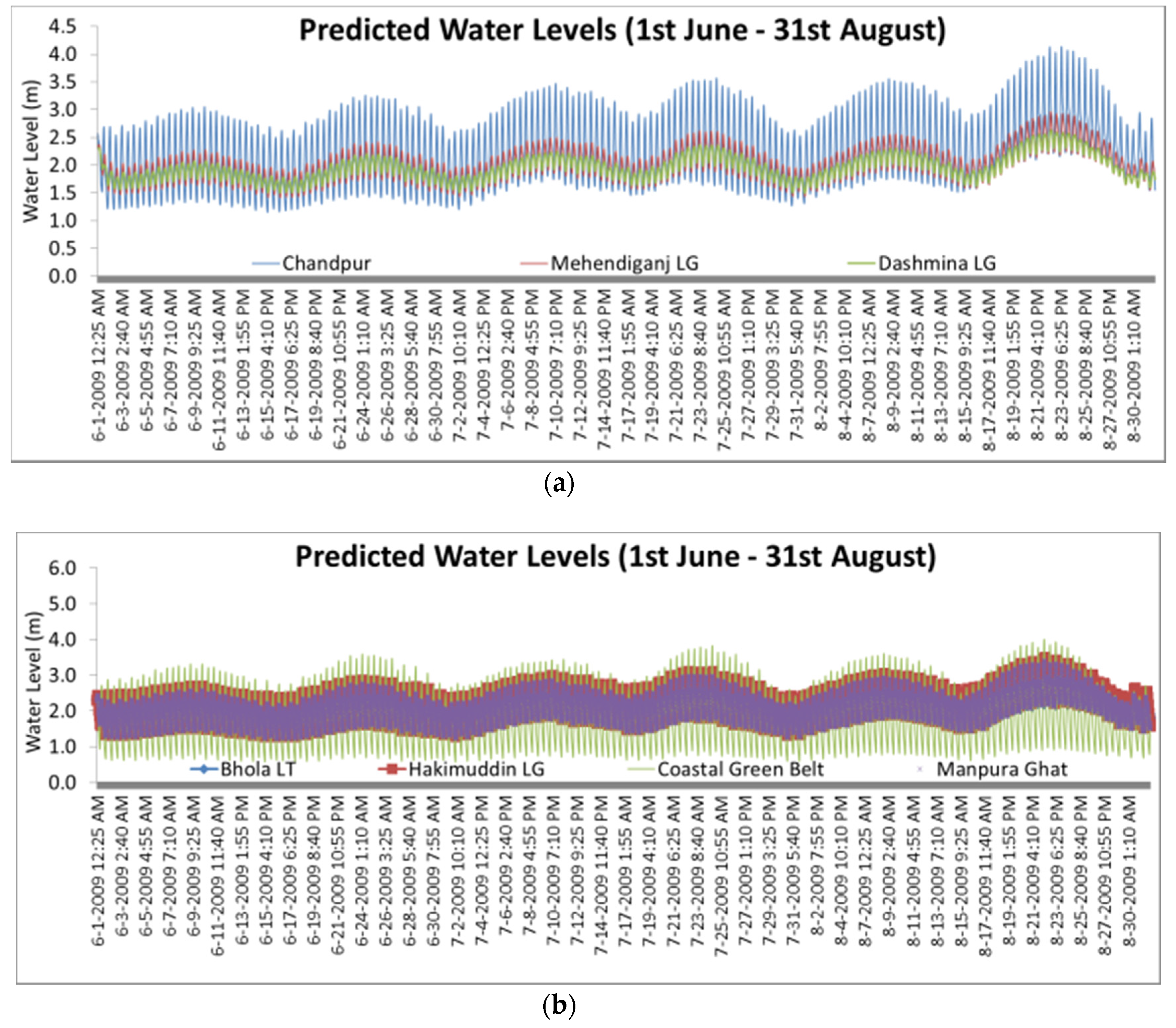
The water level prediction in un-gauged regions was precisely investigated from the point of view of a hydrodynamic model. The numerical results predicted 21 significant navigation points for the Meghna river estuary. These points were considered as un-gauged stations and as indicators of flood water levels in coastal regions. There are numerous inland water transports operating regularly among these stations. The temporal prediction of water levels indicates the tidal phase and amplitude changes recurrently within the un-gauged regions of the Meghna River estuary. Apart from the time lags among the stations, most of them are significantly correlated with the upstream water levels and sea tides (details in Section 4.2). Therefore, the water level predictions time series is shown for the rainy season in Figure 10.
The real time tidal water levels from spring to neap tide during rainy season (1 June–31 August) were clearly obtained from the hydrodynamic simulation of Chezy variable bed resistance. The results exposed that the tidal water levels in the estuary are in the range of −0.68 m to less than 4.2 m. The high water levels observed at the Chandpur station (No. 1) was 4.2 m during the spring tide on 8:40 p.m., 23 August 2009 with an east velocity (u) of −0.63 m/s, and a north velocity (v) of −1.43 m/s, a pressure flux of −8.3 m3/s/m, discharge flux of −23.5 m3/s/m, current speed of 1.61 m/s, current direction of 204.6 degrees, drag coefficient of 0.00231, and CFL number of 0.04. The minimum water level observed at the Chittagong station (No. 19) was −0.68 m during the neap tide on 8:25 a.m., 24 July 2009 with towards an east velocity (u) of −0.114 m/s, towards a north velocity (v) of −0.38 m/s, pressure flux −0.2 m3/s/m, discharge flux −0.7 m3/s/m, current speed 0.39 m/s, current direction 197.5 degree, drag coefficient 0.00561 and CFL number 0.02. The high tide was 3.88 m on 22 August 2009 at 2:55:00 p.m. at the Chittagong station.
The model prediction results indicate that water levels significantly increased between the dry and rainy season in 2009, as demonstrated in Figure 11. The blue color indicates the two boundaries, and light blue colors indicate the water level changes in the un-gauged stations. The results indicated that the water level rose 2.0 m to 4.0 m around the main channel and the coastal region of the Meghna River estuary. Conversely, 1.2 m to 1.8 m seasonal water level variations were indicated among the allied channels. The water level rise coherently occurred caused by the hydro-climatological impacts of the GBM (Ganges, Brahmaputra and Meghna) basin accumulated rainfall-runoff and the spring tide propagation during the monsoon.
4. Discussion
4.1. Numerical Model of Estuary
This study emphasized the prediction of flood water levels within the un-gauged regions of the Meghna River estuary. The assimilated physical configurations of the estuary and its boundary condition data exposed an important role for numerical methods to develop a hydrodynamic estuarine river model. To achieve the purpose of this study, a hydrodynamic model was developed, incorporating Mike21 FM, and comprising numerical and frequency analysis. This study demonstrated bathymetry configuration, empirical riverbed resistance, adjustment of boundary conditions, model calibration/validation and the prediction of water levels. Consequently, the predicted water levels of the hydrodynamic model were exposed with their relative flood return periods.
The hydrodynamic processes of tidal rivers are nonlinear and complicated, as the water level continually changes due to the interaction between upstream discharges and downstream tides. For these processes, the flow routing patterns in tidal rivers often observed to be unstable. The river discharge originates from upstream river basins, and most of the discharged water flows downstream, reaching the coastal regions and the sea. The water depth of the Meghna river estuary changed twice a day at varying times. The shallow water tides governed the estuarine river flow and the high or low water level changes the whole bathymetry. Major flow instability occurs in the confluence and tidal areas, which often results in delayed passenger ships and capsized ships in this estuary. The variations of hydrodynamic phenomena has in fact altered the flooding conditions in the whole domain. However, most analyses of the estimation of estuarine river properties suffer from a lack of real time data, a shortage of the duration of measurements, and limited gauging locations for water levels.
The predicted water level of the hydrodynamic model was compared with the observed data from a statistical linear regression model. The simulation accuracy was found to be satisfactory in terms of the confidence level, correlation and error. Previous studies were discussed and verified this regression model as an adequate statistical method for analyzing the goodness-of-fit of the data [31]. Besides water level prediction, this study also demonstrated the variations of residual flow as well as discharge fluxes. Distinctly, both inward and outward flow and pressure fluxes were caused by tides in this shallow water estuarine river. These nonlinear hydrodynamic phenomena were exposed due to spatial variation of riverbed resistance and the amplitude of semidiurnal tides. Earlier studies stated that tidally-driven river flow dynamics have relied on bed resistance and variable depth [50,51]. Inward flux was found to be high in the southern zones at those stations that are close to the bay and higher outward flux was found in the western channels and near the upstream regions. The periodical spring-to-neap tide cycle caused resilient flow fluxes. The previous studies demonstrated that flow fluxes in subtropical estuaries are high during spring tides rather than during neap tides [52]. Therefore, excessive flow fluxes may lead to flooding of the coastal land and create unusual waves in the estuary.
In the case of river modelling, river discharge and water level data observation play important roles in predictions of water levels and hydrodynamic changes at un-gauged stations. Water level measurement over time at gauging stations indicates estuarine river submerging conditions. It is a key hydrodynamic component to assess the embankment’s capacity to adapt to the negative effects of extreme hydrological changes.
The initial values of eddy viscosity (0.2 m2/s) and drag coefficient exposed non-significant effects in the model calibration. The triangulation of the gridded data and the extrapolation of the mesh, as well as the construction of the study domain, required extensive time (approx. two days). The topographic data, mesh resolution and bed roughness have a significant effect on the shallow water flow. In this study, it was found that with mesh configuration the riverbed resistance of Chezy was more efficient than Manning. In addition, three months simulation at 15-min intervals engaged approx. six days of computational time while a high configuration core-i5 processor was employed. This could occur due to the involvement of numerous finite elements in the high-resolution mesh. Due to the numerical stability (time integration and space discretization), the time step interval must be reasonably selected and the CFL number should be less than one. Therefore, the use of larger time steps influenced the numerical instability of the hydrodynamic model.
4.2. Implications of Water Level Prediction
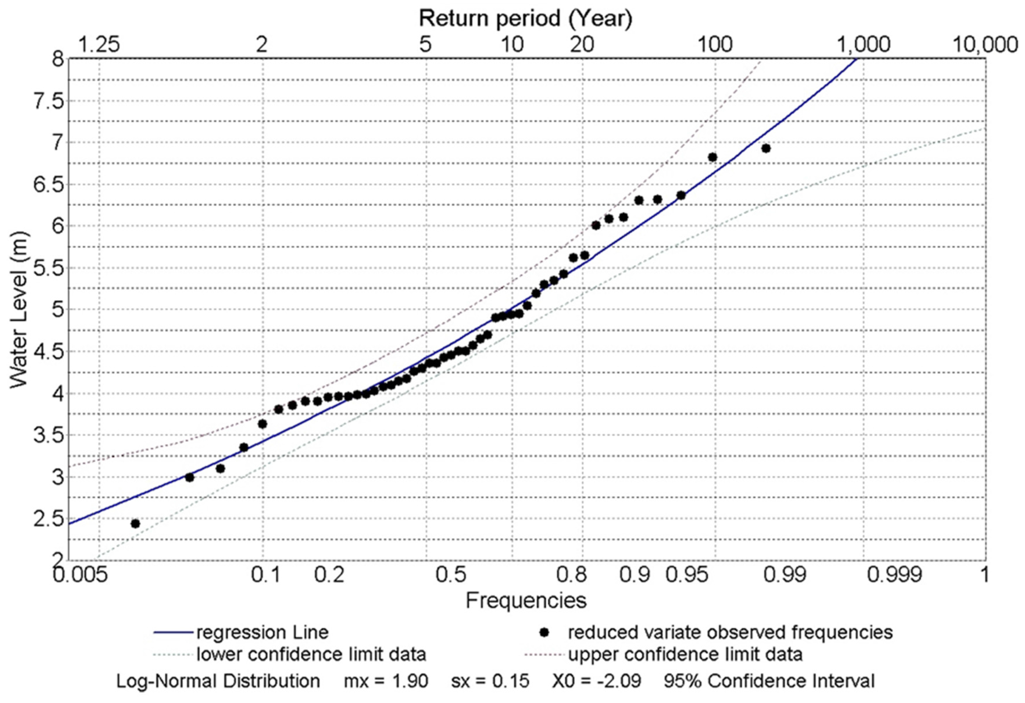
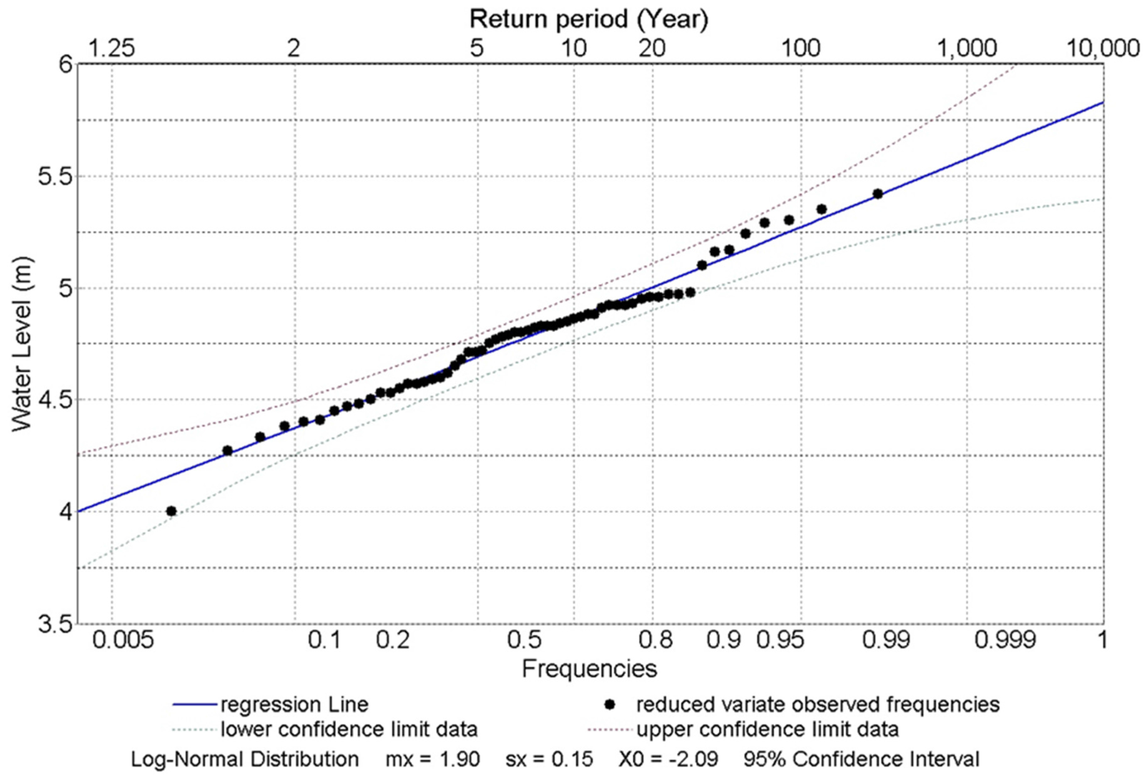
A numerical prediction procedure was applied to the water level simulation in this study. This study used a log normal distribution for the frequency analysis and returning period analysis. The probability distributions have a significant role in the assessment of flood action plans. Consequently, the Bangladesh Water Development Board’s yearly maximum observed water levels (1958–2012) were analyzed using three parameters of log normal (LN3) distribution. The goodness-of-fit of the peak water levels and corresponding return periods were determined using LN3 (95% confidence interval) and are shown in Figure 12 (Chandpur station) and Figure 13 (Chittagong station).
The difference in the peak water level at Chandpur station (upstream) between a two-year and a 100-year flood was found to be 2.7 m in the LN3 distribution. On the contrary, the difference in peak water level at the Chittagong station (sea level rise) between a two-year and a 100-year flood was found to be 1.7 m in the LN3 distribution. The dotted lines indicate the upper and lower bounds of 95% confidence. Therefore, the hydrodynamic model predicted six un-gauged station (stations 2–7) water levels, and return periods were correlated with the Chandpur station water level. Subsequently, the hydrodynamic model predicted fifteen un-gauged stations (stations 9–23); these were also correlated with the Chittagong station sea water level. This prediction and correlations indicate the flood magnitudes at the un-gauged stations of the lower Meghna river estuary as summarized in Table 3.
Most of the coastal region embankments and road elevations range 3 to 5 m above mean sea level. As a consequence, inundation occurred within the shortest return periods in the Meghna River estuary. Intergovernmental Panel on Climate Change (IPCC) stated that extreme sea level rise (SLR) would be 0.23 m in 2030s and 0.44 m in 2050s [53]. Huq et al. (1999) found that 1 m SLR will inundate 60% of Sundarban and 1.5 m SLR will require immense resettlement of 17 million (15%) people in the coastal region [54]. Hence, the development of new or existing coastal embankments/roads can prevent the coastal regions from flood inundation and these predictions and correlations would be convenient for the decision-making process.
5. Conclusions
This study exposed the applicability of hydrodynamic models for predicting water levels in the Meghna River estuary at typical ungauged river stations. The water level predictions were conducted to be applicable in both the dry and rainy seasons through physical, numerical and statistical approaches. The specific conclusions of this study are as follows:
- The hydrodynamic model produced temporal and spatial distributions of the tidal water level recurrently within the sea, main rivers, small channels, natural banks, and whole domain. The water level prediction of the hydrodynamic model was produced and evaluated, as the simulated values were compared to 126 real time observations from Chandpur river gauges.
- The hydrodynamic model was calibrated by adjusting bed resistance with the minimum prediction errors for both dry and rainy seasons, indicating seasonal differences in hydrodynamic components. Therefore, it was possible to find an optimized set of simulation factors. Moreover, this means that the results provided a possibility for their prediction, as they have shown good agreement between the data collected and the simulation results.
- Within the results generated by numerical analysis, it was possible to conduct a frequency analysis to develop a return period for upstream and downstream boundary conditions. With this analysis, it is possible to develop boundary conditions by matching them with the return period and to predict water levels for overall stations in the Meghna estuary by numerical modelling.
Acknowledgments
This research was part of a doctoral thesis. This research was supported by a grant [MOIS-DP-2015-05] through the Disaster and Safety Management Institute funded by Ministry of the Interior and Safety of Korean government.
Author Contributions
Zakir Hossein Syed led the work performance and wrote this manuscript; Seongjoon Byeon contributed to the development of the article. All research was completed with the guidance and supervision of Gyewoon Choi. All authors read and approved the final manuscript.
Conflicts of Interest
The authors declare no conflict of interest.
References
- Unite Nations Environment Programme. Unite Nations Environment Programme and Development Alternatives, South Asia Environment Outlook 2009; UNEP: Nairobi, Kenya, 2008; ISBN 978-92-807-2954-2. [Google Scholar]
- Climate Change Threat to South Asia. Available online: http://www.adb.org/features/climate-change-threat-south-asia (accessed on 14 January 2018).
- Sudhir, C.R. Blue Alert, Climate Migrants in South Asia: Estimates and Solutions; Greenpeace India: Bangalore, India, 2008. [Google Scholar]
- Hossain, M. Global Warming Induced Sea Level Rise on Soil, Land and Crop Production Loss in Bangladesh. In Proceedings of the 19th World Congress of Soil Science, Brisbane, Australia, 1–6 August 2010; pp. 77–80. [Google Scholar]
- Unite Nations Environment Programme (UNEP). Vital Water Graphics: An Overview of the State of the World’s Fresh and Marine Waters, 2nd ed.; UNEP: Nairobi, Kenya, 2008; ISBN 92-807-2236-0. [Google Scholar]
- Taormina, R.; Chau, K.W.; Sivakumar, B. Neural network river forecasting through baseflow separation and binary-coded swarm optimization. J. Hydrol. 2015, 529, 1060–1069. [Google Scholar] [CrossRef]
- Wu, C.L.; Chau, K.W.; Fan, C. Prediction of rainfall time series using modular artificial neural networks coupled with data-preprocessing techniques. J. Hydrol. 2010, 389, 146–167. [Google Scholar] [CrossRef]
- Wang, W.C.; Chau, K.W.; Xu, D.; Qiu, L.; Liu, C. The annual maximum flood peak discharge forecasting using Hermite projection pursuit regression with SSO and LS method. Water Resour. Manag. 2017, 31, 461–477. [Google Scholar] [CrossRef]
- Chen, X.Y.; Chau, K.W.; Busari, A.O. A comparative study of population-based optimization algorithms for downstream river flow forecasting by a hybrid neural network model. Eng. Appl. Artif. Intell. 2015, 46, 258–268. [Google Scholar] [CrossRef]
- Chau, K.W.; Wu, C.L. A hybrid model coupled with singular spectrum analysis for daily rainfall prediction. J. Hydroinfrom. 2010, 12, 458–473. [Google Scholar] [CrossRef]
- Ahmed, M. Development and management challenges of integrated planning for sustainable productivity of water resources. Bangladesh J. Political Econ. 2004, 21, 2. [Google Scholar]
- Mirza, M.M.Q. Climate change, flooding in South Asia and implications. Reg. Environ. Chang. 2011, 11, 95–107. [Google Scholar] [CrossRef]
- Dasgupta, S.; Laplante, B.; Murray, S.; Wheeler, D. Sea-Level Rise and Storm Surges: A Comparative Analysis of Impacts in Developing Countries; World Bank: Washington DC, USA, 2009; pp. 27–41. [Google Scholar]
- Khalequzzaman, M. Flood Control in Bangladesh through Best Management Practices. In Proceedings of the SAARC Workshop on Flood Risk Management in South Asia, Islamabad, Pakistan, 9–10 October 2012. [Google Scholar]
- Klassen, G.J.; Douben, K.J.; Waal, M.V.D. Novel Approaches in River Engineering. In The River Flow, Proceedings of the International Conference on Fluvial Hydraulics, Louvain la Neuve, Belgium, 4–6 September 2002; Bousmar, D., Zech, Y., Eds.; pp. 27–43.
- Siddique, K.A.B. Evaluation of Chandpur Town Protection. Master’s Thesis, Department of Water Resources Engineering, Bangladesh University of Engineering and Technology, Dhaka, Bangladesh, 2004. [Google Scholar]
- Karim, M.F.; Mimura, N. Impacts of climate change and sea-level rise on cyclonic storm surge floods in Bangladesh. Int. J. Glob. Environ. Chang. 2008, 18, 490–500. [Google Scholar] [CrossRef]
- Bangladesh Water Development Board (BWDB). Meghna Estuary Study 1999; Main Report; DGIS/DANIDA/GOB; BWDB: Dhaka, Bangladesh, 1999; Volume 1, p. 8.
- Allison, M.A. Historical changes in the Ganges-Brahmaputra delta front. J. Coast. Res. 1998, 14, 1269–1275. [Google Scholar]
- Dube, S.K.; Rao, A.D.; Sinha, P.C.; Murty, T.S.; Bahulayan, N. Storm surge in the Bay of Bengal and Arabian Sea: The problem and its prediction. Mausam 1997, 48, 283–304. [Google Scholar]
- Murty, T.S.; Flather, R.A.; Henry, R.F. The storm surge problem in the Bay of Bengal. Prog. Oceanogr. 1986, 16, 195–233. [Google Scholar] [CrossRef]
- Mcinnes, K.L.; Walsh, K.J.E.; Hubbert, G.D.; Beer, T. Impact of sea-level rise and storm surges on a coastal community. Nat. Hazards 2003, 30, 187–207. [Google Scholar] [CrossRef]
- Huang, W.; Spaulding, M. 3D model of estuarine circulation and water quality induced by surface discharges. ASCE J. Hydraul. Eng. 1995, 121, 300–311. [Google Scholar] [CrossRef]
- Liang, D.; Falconer, R.A.; Lin, B. Comparison between TVD-MacCormack and ADI-Type Solvers of the Shallow Water Equations. Adv. Water Res. 2006, 29, 1833–1845. [Google Scholar] [CrossRef]
- Mendelsohn, D.L.; Swanson, J.C. Application of a boundary fitted coordinate mass transport model. In Proceedings of the 2nd International Conference on Estuarine and Coastal Modeling, ASCE, Tampa, FL, USA, 13–15 November 1991. [Google Scholar]
- Spaulding, M.L. A vertically averaged circulation model using boundary-fitted coordinates. J. Phys. Oceanogr. 1984, 14, 973–982. [Google Scholar] [CrossRef]
- DHI. MIKE 21: Coastal Hydraulics and Oceanography—User Guide; DHI Water and Environment: Hørsholme, Denmark, 2007; p. 204. [Google Scholar]
- Jones, O.P.J. Modelling Headland Sandbank Dynamics. Ph.D. Thesis, Department Civil & Environmental Engineering, University College London, London, UK, 2007. [Google Scholar]
- Zahid Ahmed, M.M.; Mahboob-Ul-Kabir, M.D.; Abdul Hye, J.M. Hydraulic Mathematical Modelling for Proposed Riverbank Protection Works at Himchar Area. In Proceedings of the 6th Intertional Conference on Hydroinform, Singapore, 21–24 June 2004. [Google Scholar]
- Soulsby, R.L. Dynamics of Marine Sands; Thomas Telford Publications: London, UK, 1997; p. 249. [Google Scholar]
- Amemiya, T. Selection of regressors. Int. Econ. Rev. 1980, 21, 331–354. [Google Scholar] [CrossRef]
- Dutta, D.; Alam, J.; Umeda, K.; Hayashi, M.; Hironaka, S. A two-dimensional hydrodynamic model for flood inundation simulation: A case study in the lower Mekong river basin. J. Hydrol. Proc. 2007, 21, 1223–1237. [Google Scholar] [CrossRef]
- Yue, Z.Y.; Cao, Z.X.; Li, X.; Che, T. Two-dimensional coupled mathematical modeling of fluvial processes with intense sediment transport and rapid bed evolution. Sci. China Ser. G-Phys. Mech. Astron. 2008, 51, 1427–1438. [Google Scholar] [CrossRef]
- Hardy, R.J.; Bates, P.D.; Anderson, M.G. The importance of spatial resolution in hydraulic modelling of floodplain environments. J. Hydrol. 1999, 216, 124–136. [Google Scholar] [CrossRef]
- Horritt, M.S. Development of physically based meshes for two-dimensional models of meandering channel flow. Int. J. Numer. Methods Eng. 2000, 47, 2019–2037. [Google Scholar] [CrossRef]
- Horritt, M.S. Development and testing of a simple two dimensional finite volume model of sub-critical shallow water flow. Int. J. Numer. Methods Fluids 2004, 44, 1231–1255. [Google Scholar] [CrossRef]
- Horritt, M.S.; Bates, P.D.; Mattinson, M.J. Effects of mesh resolution and topographic representation in 2D finite volume models of shallow water fluvial flow. J. Hydrol. 2006, 329, 306–314. [Google Scholar] [CrossRef]
- Sinnakaudan, S.K. Integrated Triangular Irregular Network (ITIN) Model for flood plain analysis. Int. J. Geoinform. 2009, 5, 47–55. [Google Scholar]
- Kubatko, E.J.; Dawson, C.; Conroy, C.J.; Maggi, A.L. A sigma-coordinate, discontinuous Galerkin method for the three-dimensional shallow water equations. In Proceedings of the 9th International Workshop on Multiscale (Un)-Structured Mesh Numerical MODELING for Coastal, Shelf, and Global Ocean Dynamics, Cambridge, MA, USA, 17–20 August 2010. [Google Scholar]
- Liang, D.; Binliang, L.; Falconer, R.A. Simulation of rapidly varying flow using an efficient TVD-MacCormack scheme. Int. J. Numer. Methods Fluids 2007, 53, 811–826. [Google Scholar] [CrossRef]
- Huttunen, J.; Lehikoinen, A.; Hamalainen, J.; Kaipio, J. Importance filtering approach for the nonstationary approximation error method. Inverse Probl. 2010, 26, 16. [Google Scholar] [CrossRef]
- Romanowicz, R.J.; Young, P.C.; Beven, K.J. Data assimilation and adaptive forecasting of water levels in the river Severn catchment. U. K. Water Resour. Res. 2006, 42, W06407. [Google Scholar] [CrossRef]
- Wu, Q.; Litrico, X.; Bayen, A. Data reconciliation of an open channel flow net-838 work using a modal decomposition. J. Adv. Water Resour. 2009, 32, 193–204. [Google Scholar] [CrossRef]
- Reddy, M.P.M.; Affholder, M. Descriptive Physical Oceanography: State of the Art; Taylor and Francis: Didcot, UK, 2002; p. 249. ISBN 90-5410-706-5. [Google Scholar]
- Bartels, R.H.; Beatty, J.C.; Barsky, B.A. Hermite and Cubic Spline Interpolation. An Introduction to Splines for Use in Computer Graphics and Geometric Modelling; Morgan Kaufmann: San Francisco, CA, USA, 1987; pp. 9–17. ISBN 1-55860-400-6. [Google Scholar]
- John, H.M.; Kurtis, K.F. Numerical Methods Using Matlab, 4th ed.; Prentice-Hall Inc.: Upper Saddle River, NJ, USA, 2004; ISBN 0-13-065248-2. [Google Scholar]
- Hussain, M.A.; Tajima, Y.; Taguchi, Y.; Gunasekara, K. Tidal characteristics affected by dynamic morphology change in the meghna estuary. In Proceedings of the 7th International Conference on Asian and Pacific Coasts, Bali, Indonesia, 24–26 September 2013. [Google Scholar]
- Wilde, D.K. Moving Coastlines: Emergence and Use of Land in the Ganges-Brahmaputra-Meghna Estuary; University Press Limited: Dhaka, Bangladesh, 2011. [Google Scholar]
- Zakir, S.H.; Gyewoon, C. Prediction of water level using hydrodynamic model for lower Meghna river estuary in Bangladesh. In Proceedings of the 1st International Conference on Smart Water Grid, Incheon, Korea, 12–14 November 2013. [Google Scholar]
- Li, C.; Chen, C.; Guadagnoli, D.; Georgiou, I.Y. Geometry-induced residual eddies in estuaries with curved channels: Observations and modeling studies. J. Geophys. Res. 2008, 113, C01005. [Google Scholar] [CrossRef]
- Winant, C.D. Three-dimensional residual tidal circulation in an elongated, rotating basin. J. Phys. Oceanogr. 2008, 38, 1278–1295. [Google Scholar] [CrossRef]
- Valle-Levinson, A.; Gutierrez, D.V.G.; Trasvina, A.; Souza, A.; Durazo, R.; Mehta, A. Residual exchange flows in subtropical estuaries. J. Estuar. Coasts 2009, 32, 54–67. [Google Scholar] [CrossRef]
- Thomas, T.; Ahmadul, H.; Nabiul, I.K.M.; Declan, C.; Reinhard, M.; Ahsan, U.A.; Mozaharul, A. The ORCHID: Piloting Climate Risk Screening in DFID Bangladesh; Detailed Research Report; Institute of Development Studies: Brighton, UK, 2007. [Google Scholar]
- Huq, S.; Karim, Z.; Asaduzzaman, M.; Mahtab, F. Vulnerability and Adaptation to Climate Change for Bangladesh; Kluwer Academic Publishers: London, UK, 1999; pp. 39–54. ISBN 978-94-015-9325-0. [Google Scholar]
Figure 1.
Study area, river and tidal gauge stations.
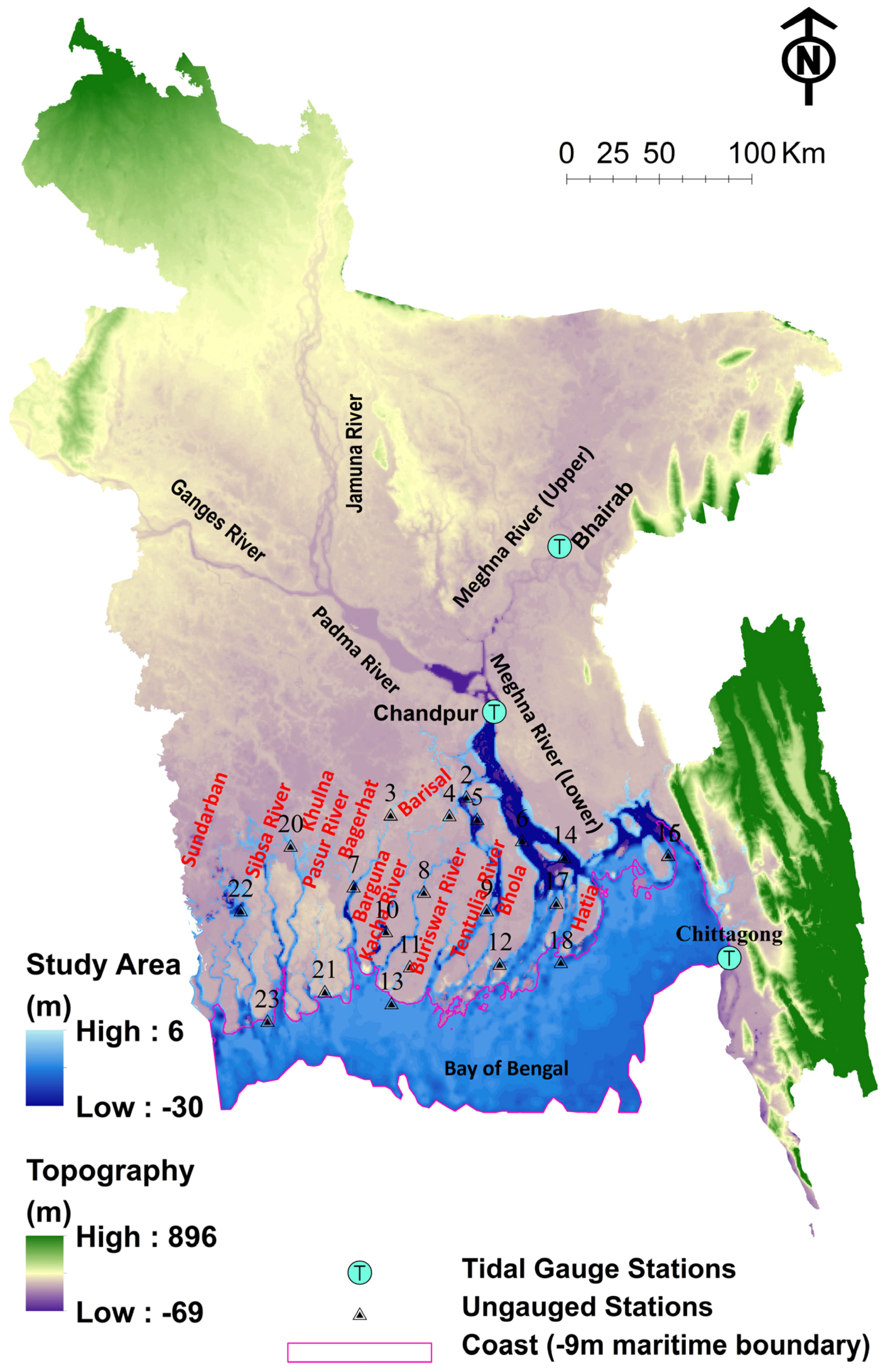
Figure 2.
Computational domain in BTM projection (a) domain boundaries; (b) triangulation of study domain; (c) bathymetry with triangulated domain; and (d) computation bathymetry.
Figure 2.
Computational domain in BTM projection (a) domain boundaries; (b) triangulation of study domain; (c) bathymetry with triangulated domain; and (d) computation bathymetry.

Figure 3.
Boundary conditions (a) tide level in dry season; (b) tide level in rainy season at Chittagong station; (c) discharge in dry season; and (d) discharge in rainy season at Chandpur station.
Figure 3.
Boundary conditions (a) tide level in dry season; (b) tide level in rainy season at Chittagong station; (c) discharge in dry season; and (d) discharge in rainy season at Chandpur station.

Figure 4.
The goodness of fit for the dry season, (a) water level calculated by Manning’s equation vs. observed water level and (b) water level calculated by the Chezy equation vs. observed water levels at Chandpur station.
Figure 4.
The goodness of fit for the dry season, (a) water level calculated by Manning’s equation vs. observed water level and (b) water level calculated by the Chezy equation vs. observed water levels at Chandpur station.

Figure 5.
The goodness of fit for the rainy season, (a) water level by constant Manning m vs. observed water level and (b) variable Manning’s m vs. observed, (c) constant Chezy c vs. observed and (d) variable Chezy c vs. observed water level at Chandpur station.
Figure 5.
The goodness of fit for the rainy season, (a) water level by constant Manning m vs. observed water level and (b) variable Manning’s m vs. observed, (c) constant Chezy c vs. observed and (d) variable Chezy c vs. observed water level at Chandpur station.

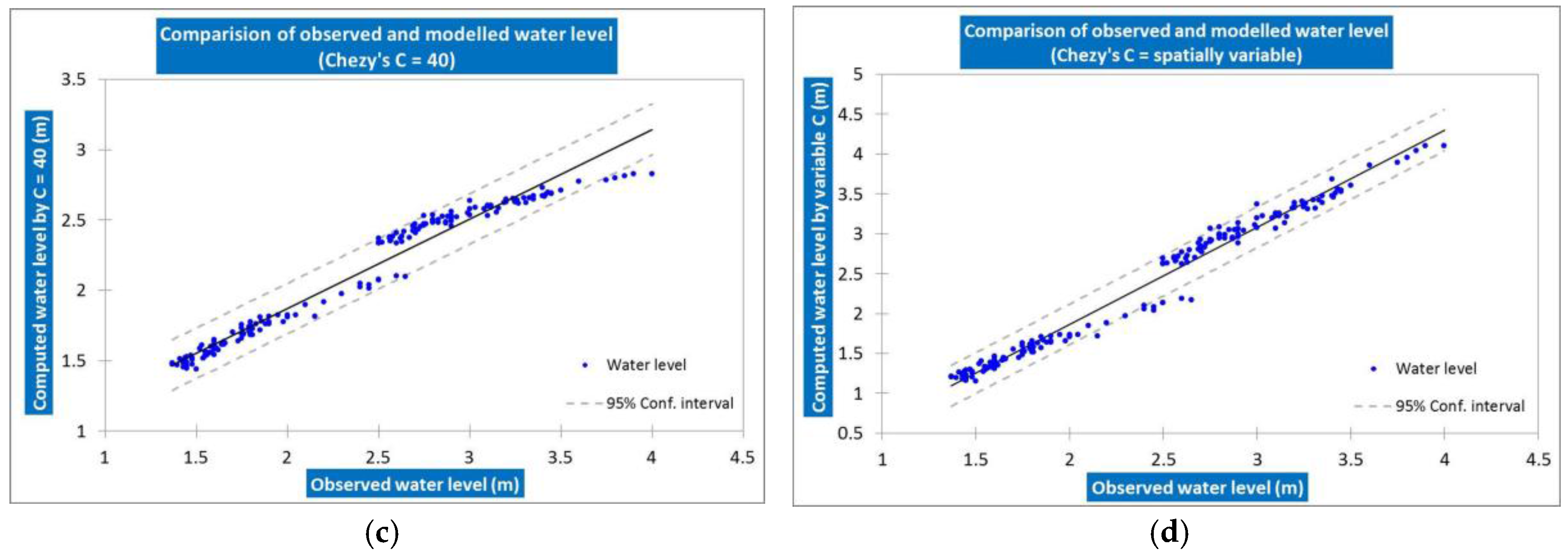
Figure 6.
The variation of pressure flux for the un-gauged stations of Meghna river estuary (a) Mehendiganj LG and Dashmina (b) Bhola, Hakimuddin, Coastal Green Belt and Manpura Ghat.
Figure 6.
The variation of pressure flux for the un-gauged stations of Meghna river estuary (a) Mehendiganj LG and Dashmina (b) Bhola, Hakimuddin, Coastal Green Belt and Manpura Ghat.
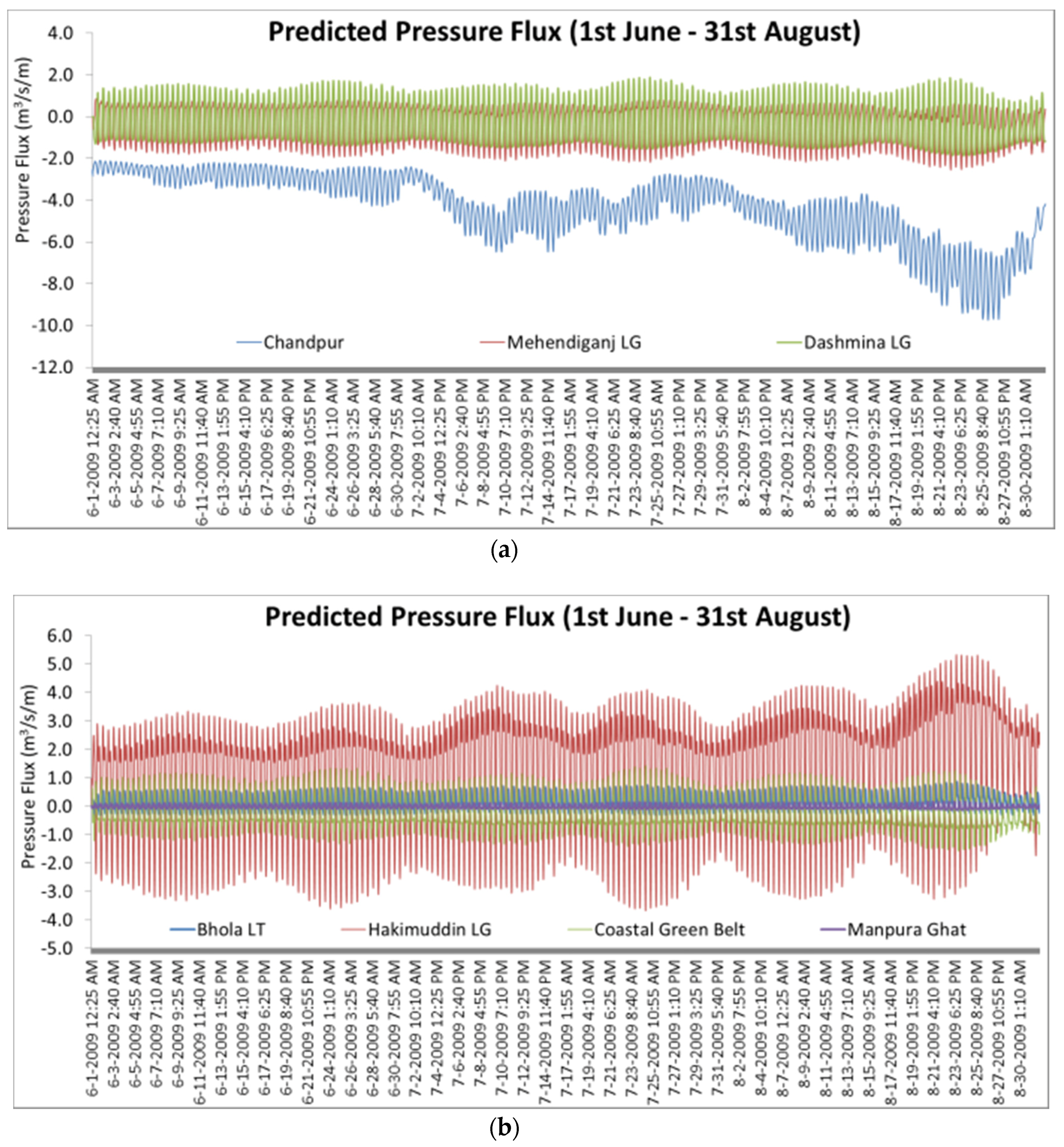
Figure 7.
Discharge fluxes of the Meghna river estuary (a) Chandpur, Mehendiganj LG and Dashmina (b) Bhola LT, Hakimuddin LG, Coastal Green Belt and Manpura Ghat.
Figure 7.
Discharge fluxes of the Meghna river estuary (a) Chandpur, Mehendiganj LG and Dashmina (b) Bhola LT, Hakimuddin LG, Coastal Green Belt and Manpura Ghat.
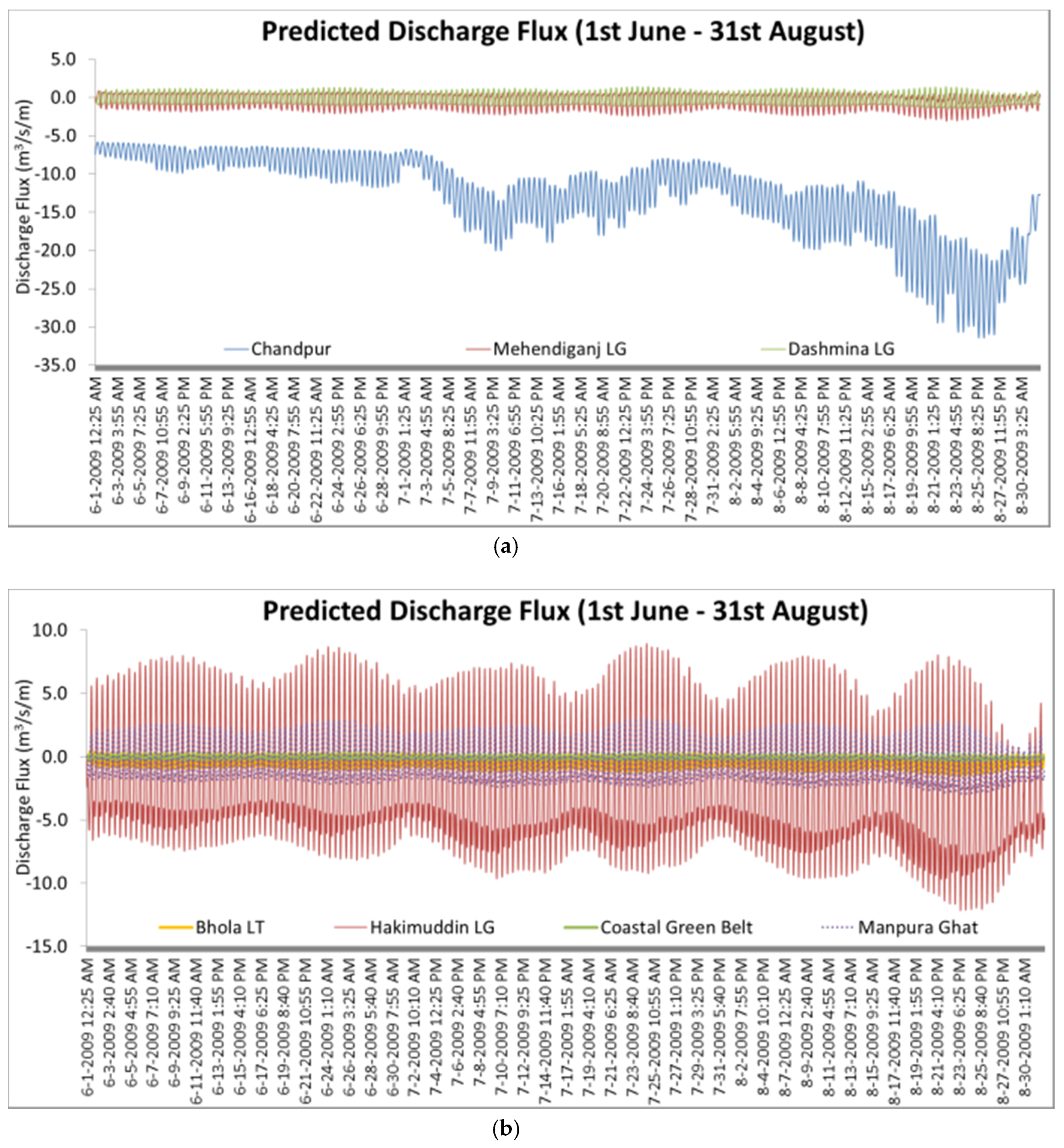
Figure 8.
Spatial variation at spring tide on 22 August 2009 at 2:55 p.m. (a) surface elevation (EL + m); (b) total water depth (m); (c) current speed (m/s); and (d) current direction (degree).
Figure 8.
Spatial variation at spring tide on 22 August 2009 at 2:55 p.m. (a) surface elevation (EL + m); (b) total water depth (m); (c) current speed (m/s); and (d) current direction (degree).
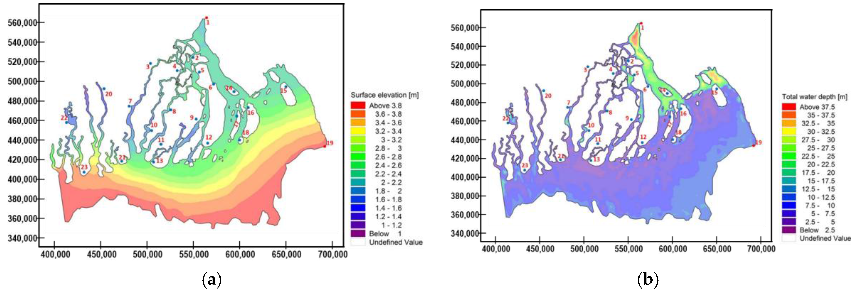
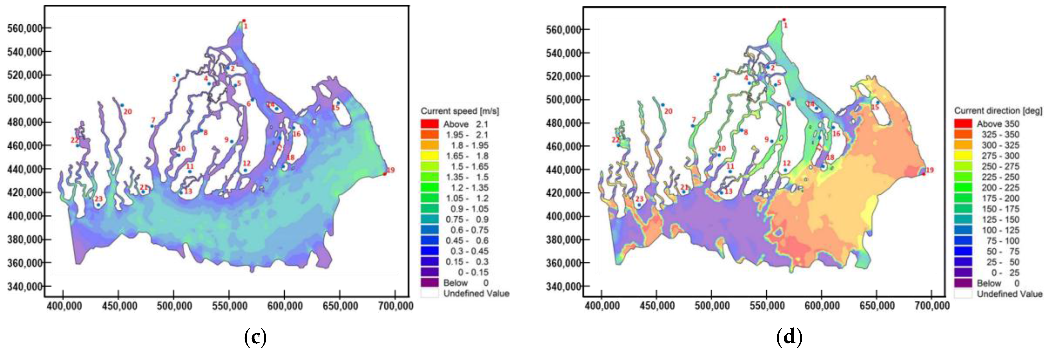
Figure 9.
Spatial variation at neap tide on 23 August 2009 at 10:40 p.m. (a) surface elevation (EL + m); (b) total water depth (m); (c) current speed (m/s); and (d) current direction (degree).
Figure 9.
Spatial variation at neap tide on 23 August 2009 at 10:40 p.m. (a) surface elevation (EL + m); (b) total water depth (m); (c) current speed (m/s); and (d) current direction (degree).
Figure 10.
The predicted water levels for the un-gauged stations of the Meghna river estuary (a) Mehendiganj LG and Dashmina (b) Bhola, Hakimuddin, Coastal Green Belt and Manpura Ghat.
Figure 10.
The predicted water levels for the un-gauged stations of the Meghna river estuary (a) Mehendiganj LG and Dashmina (b) Bhola, Hakimuddin, Coastal Green Belt and Manpura Ghat.

Figure 11.
Seasonal water level changes in gauged and un-gauged stations—Meghna river estuary.
Figure 12.
Water level returning period and frequencies for water level prediction at the upstream Chandpur station.
Figure 12.
Water level returning period and frequencies for water level prediction at the upstream Chandpur station.

Figure 13.
Water level returning period and frequencies for water level prediction at the downstream Chittagong station.
Figure 13.
Water level returning period and frequencies for water level prediction at the downstream Chittagong station.


Table 1.
Goodness of numerical decision for dry season at Chandpur station (two cases).
| Fitting Parameter | Chandpur Station | |
|---|---|---|
| Manning Variable (Ripple Sand) | Chezy Variable (Ripple Sand) | |
| Observation | 62 | 62 |
| R2 | 0.988 | 0.997 |
| MSE (m) | 0.003 | 0.001 |
| RMSE (m) | 0.055 | 0.035 |
| MAPE (%) | 2.216 | 2.014 |
Table 2.
Goodness of numerical decision for rainy season at Chandpur station (four cases).
| Fitting Parameter | Manning Constant (35) | Chezy Constant (40) | Manning Variable (Ripple Sand) | Chezy Variable (Ripple Sand) |
|---|---|---|---|---|
| Observations | 174 | 174 | 174 | 174 |
| R² | 0.954 | 0.967 | 0.968 | 0.983 |
| MSE (m) | 0.017 | 0.007 | 0.012 | 0.013 |
| RMSE (m) | 0.130 | 0.084 | 0.111 | 0.115 |
| MAPE (%) | 4.981 | 3.012 | 3.919 | 3.885 |
Table 3.
Outcomes of un-gauged station water level predictions.
| St. No | Name | East | North | ∆t * (h) | Predicted Water Level (m) | Water Level Return Periods (Year) | |||||
|---|---|---|---|---|---|---|---|---|---|---|---|
| 2 | 5 | 10 | 25 | 50 | 100 | ||||||
| 1 | Chandpur | 564,000 | 569,500 | 5:00 | 4.13 | 3.98 | 4.44 | 5.08 | 6.22 | 6.38 | 6.70 |
| 2 | Mehendiganj LG | 549,000 | 523,600 | 6:30 | 2.97 | 2.87 | 3.20 | 3.66 | 4.48 | 4.59 | 4.82 |
| 3 | Sharupkathi LG | 508,000 | 513,900 | 6:00 | 2.51 | 2.43 | 2.71 | 3.10 | 3.80 | 3.89 | 4.09 |
| 4 | Barisal SG | 539,800 | 513,600 | 6:30 | 3.02 | 2.91 | 3.24 | 3.71 | 4.54 | 4.66 | 4.89 |
| 5 | Bhola LT | 554,800 | 511,600 | 6:45 | 2.96 | 2.83 | 3.15 | 3.61 | 4.42 | 4.53 | 4.76 |
| 6 | Hakimuddin LG | 579,000 | 500,000 | 4:30 | 3.49 | 3.19 | 3.55 | 4.07 | 4.98 | 5.10 | 5.36 |
| 7 | Sarankhola LG | 488,000 | 475,000 | 4:15 | 2.79 | 2.69 | 3.00 | 3.43 | 4.20 | 4.31 | 4.52 |
| 8 | Chittagong | 691,000 | 436,000 | 0:00 | 3.88 | 3.84 | 4.92 | 5.02 | 5.22 | 5.29 | 5.50 |
| 9 | Dashmina LG | 560,000 | 462,000 | 7:00 | 2.64 | 2.62 | 2.66 | 2.72 | 2.83 | 2.87 | 2.98 |
| 10 | Barguna FG | 505,500 | 450,600 | 3:15 | 3.1 | 3.05 | 3.10 | 3.16 | 3.29 | 3.33 | 3.47 |
| 11 | Kalapara FT | 518,500 | 431,600 | 2:45 | 3.24 | 3.22 | 3.27 | 3.34 | 3.47 | 3.52 | 3.66 |
| 12 | Coastal Green Belt | 567,000 | 433,000 | 2:30 | 4 | 3.97 | 4.03 | 4.12 | 4.28 | 4.34 | 4.51 |
| 13 | Kuakata FP | 508,500 | 411,600 | 1:30 | 3.61 | 3.58 | 3.64 | 3.72 | 3.86 | 3.92 | 4.07 |
| 14 | Hatia Island | 602,000 | 491,000 | 3:30 | 3.28 | 3.24 | 3.29 | 3.36 | 3.50 | 3.55 | 3.69 |
| 15 | Sandip Beach | 658,000 | 492,000 | 2:00 | 3.65 | 3.63 | 3.69 | 3.77 | 3.92 | 3.97 | 4.13 |
| 16 | Tojumoddin LG | 658,000 | 492,000 | 3:00 | 3.4 | 3.39 | 3.44 | 3.52 | 3.66 | 3.71 | 3.85 |
| 17 | Manpura Ghat | 597,500 | 466,000 | 3:15 | 3.4 | 3.36 | 3.42 | 3.49 | 3.63 | 3.68 | 3.82 |
| 18 | Nijhum Dip Beach | 600,000 | 434,000 | 1:45 | 3.81 | 3.77 | 3.83 | 3.92 | 4.07 | 4.13 | 4.29 |
| 19 | Patuakhali SG | 526,000 | 472,000 | 4:30 | 2.68 | 2.66 | 2.70 | 2.76 | 2.87 | 2.91 | 3.03 |
| 20 | Mongla Port | 454,000 | 497,000 | 5:00 | 2.74 | 2.71 | 2.75 | 2.81 | 2.92 | 2.96 | 3.08 |
| 21 | Sundarban Pasur | 472,500 | 418,000 | 1:30 | 3.64 | 3.63 | 3.69 | 3.77 | 3.92 | 3.97 | 4.13 |
| 22 | Sundarban Dumuria LG | 427,000 | 462,000 | 4:45 | 2.36 | 2.33 | 2.37 | 2.42 | 2.52 | 2.55 | 2.65 |
| 23 | Sundarban Hiron Point | 441,500 | 402,000 | 1:00 | 3.91 | 3.87 | 3.93 | 4.02 | 4.18 | 4.23 | 4.40 |
* ∆t with sea tide (Chittagong), L = Launch G = Ghat, S = Steamer, F = Ferry, T = Terminal.
© 2018 by the authors. Licensee MDPI, Basel, Switzerland. This article is an open access article distributed under the terms and conditions of the Creative Commons Attribution (CC BY) license (http://creativecommons.org/licenses/by/4.0/).
Share and Cite
MDPI and ACS Style
Syed, Z.H.; Choi, G.; Byeon, S. A Numerical Approach to Predict Water Levels in Ungauged Regions—Case Study of the Meghna River Estuary, Bangladesh. Water 2018, 10, 110. https://doi.org/10.3390/w10020110
AMA Style
Syed ZH, Choi G, Byeon S. A Numerical Approach to Predict Water Levels in Ungauged Regions—Case Study of the Meghna River Estuary, Bangladesh. Water. 2018; 10(2):110. https://doi.org/10.3390/w10020110
Chicago/Turabian StyleSyed, Zakir Hossein, Gyewoon Choi, and Seongjoon Byeon. 2018. "A Numerical Approach to Predict Water Levels in Ungauged Regions—Case Study of the Meghna River Estuary, Bangladesh" Water 10, no. 2: 110. https://doi.org/10.3390/w10020110
Note that from the first issue of 2016, this journal uses article numbers instead of page numbers. See further details here.