Spatial and Temporal Analysis of Rainfall Concentration Using the Gini Index and PCI
by
 ,
,
Claudia Sangüesa
1, 
Roberto Pizarro
1,
Alfredo Ibañez
1,
Juan Pino
1,
Diego Rivera
2 ,
,
Pablo García-Chevesich
3,4,5,* and
Ben Ingram
6
1
Technological Center of Environmental Hydrology, University of Talca, Talca 3462227, Chile
2
Department of Water Resources, University of Concepción, Chillán 3812120, Chile
3
Faculty of Forest Sciences and Nature Conservancy, University of Chile, Santiago 8820808, Chile
4
Department of Hydrology and Atmospheric Sciences & Department of Agricultural and Biosystems Engineering, University of Arizona, Tucson, AZ 85721, USA
5
International Hydrological Programme & International Sediment Initiative, UNESCO, Montevideo 11#00 & 12#00, Uruguay
6
School of Water, Energy and Environment, Cranfield University, College Rd, Cranfield MK43 0AL, UK
*
Author to whom correspondence should be addressed.
Water 2018, 10(2), 112; https://doi.org/10.3390/w10020112
Submission received: 16 November 2017
/
Revised: 22 January 2018
/
Accepted: 22 January 2018
/
Published: 28 January 2018
Abstract
:This study aims to determine if there is variation in precipitation concentrations in Chile. We analyzed daily and monthly records from 89 pluviometric stations in the period 1970–2016 and distributed between 29°12′ S and 39°30′ S. This area was divided into two climatic zones: arid–semiarid and humid–subhumid. For each station, the Gini coefficient or Gini Index (GI), the precipitation concentration index (PCI), and the maximum annual precipitation intensity in a 24-h duration were calculated. These series of annual values were analyzed with the Mann–Kendall test with 5% error. Overall, it was noted that positive trends in the GI are present in both areas, although most were not found to be significant. In the case of PCI, the presence of positive trends is only present in the arid–semiarid zone; in the humid–subhumid zone, negative trends were mostly observed, although none of them were significant. Although no significant changes in all indices are evident, the particular case of the GI in the humid–subhumid zone stands out, where mostly positive trends were found (91.1%), of which 35.6% were significant. This would indicate that precipitation is more likely to be concentrated on a daily scale.
1. Introduction
In recent years, on a global scale, there have been marked climatic variations that have influenced the spatio-temporal behavior of meteorological variables such as precipitation (mean, extreme, variability) [1,2]. Understanding future changes in the frequency, intensity, and duration of extreme events is important when formulating adaptation and mitigation strategies that minimize damage to natural and human systems [3]. Indeed, Zubieta & Saavedra [4] point out that one of the most important aspects of climate change that requires in-depth research is the characterization of precipitation in time and space.
Chile is not immune to climate change and variability, because the country has distinct climate types that vary from north to south. The Pacific anticyclone generally manifests itself in the northern territory of the country which causes a lack of rainfall that leads to arid and semi-arid conditions. As one moves southwards, the influence of cold air masses manifest (commonly referred as ‘polar fronts’ due to their origin), which when interacting with warm air masses, they produce intense rainfall events [5,6]. This is why there is an extremely arid environment in the north of the country, while the south is humid. Therefore, if the country faces a phenomenon of climate change or high climatic variability, precipitation would be highly sensitive to these phenomena, because Chile is located in a climatic transition zone [7,8]. In contrast, rainfall in the central-southern part of the country is related to the dynamics of some events, such as El Niño–Southern Oscillation (ENSO) [9], which generally presents a warm phase in central Chile (30° S–35° S) associated with an increase in winter rainfall. In the southern zone (38° S–41° S), events are usually linked to reduced rainfall, especially in the following summer [10,11,12,13,14,15,16]. Nevertheless, in non-ENSO conditions there are several processes that generate rainfall in winter, such as blocking and orographic effects [17].
Both, the distribution and intensity of precipitation, as well as geomorphology, among other aspects, determine the sensitivity of the territory to meteorological hazards triggered by excessive levels of rainfall. These events can occur in the form of flooding of riverbeds, floods, alluvial floods, avalanches, landslides, and swells on coasts [18]. In this context, Favier et al. [19] noted that precipitation in the semiarid North Chico region of Chile, after a considerable decline before 1930, has remained almost unchanged to date. Likewise, Sarricolea & Romero [20] describe that precipitation trends in the arid zone of the Chilean plateau show a sharp decrease. The same situation is occurring in the humid–subhumid zone of the country, observing negative trends of rainfall [21] and a higher precipitation concentration in winter [12].
Precipitation concentration—i.e., a measure of temporal distribution of precipitation in a location—can be characterized by different models such as the Gini index (GI), the concentration index (CI) [22,23], and the precipitation concentration index (PCI) [24,25]. The first method is used to establish and assess the unequal distribution of precipitation. Martin-Vide [26] developed the concentration index (CI), which represents the theoretical frequency of the data. Similarly, the Gini index can also be used on the complete data series, or only on days with precipitation. Finally, the PCI assesses precipitation concentration based on the variability of monthly precipitation.
Research in Chile indicates that the CI has increased, verifying that rainfall occurs on fewer days of the year, with the arid region showing the highest value [22,27,28]. Pizarro et al. [25] and Valdés-Pineda et al. [15] verify the existence of certain trends, however these trends do not necessarily imply an explicit change in precipitation concentration. The high temporal concentration of precipitation is linked to the rapid rate of physical processes, such as convection in areas with a high degree of exposure to sunlight and warmer seas. In turn, the low rainfall concentration can be interpreted as a consequence of regular patterns (sea currents or highly recurrent storms) [22].
Similarly, a rainfall concentration study was developed in Mediterranean climates of Spain, using the PCI and considering a time period between 1946 and 2005 [29]. The authors concluded an annual increase of PCI values, a conclusion that was explained by an increase of winter precipitations. Using the CI, on the other hand, Li et al. [30] evaluated the concentration of daily rainfall and its trends in 50 meteorological stations in Xinjiang, northwest China. Although a spatial pattern was found in the daily concentration of rainfall, trends were not significant. Finally, a global rainfall concentration analysis was performed by Raha et al. [31], who analyzed 12,513 stations for the 1976–2000 period, using the Gini index (wet days). The index was analyzed through linear regressions, with negative trends (mostly) in South Asia, Central America, and Brazil, while trends were positive in the rest of South America.
In recent years, significant events have occurred in Chile that have caused natural disasters with human life, and economic and infrastructural losses. The disasters that have the greatest impact on the country have been mostly seismic (earthquakes and tsunamis) and climatic (droughts and floods). In the Mediterranean zone (32° S–38° S), floods are related to the presence of cold and warm frontal systems. Of the 227 river flood events recorded in Chile within the 1574–2012 period, 71% of them are associated with intense or persistent rainfall events [32].
As previously mentioned, hydrological variables are sensitive to rainfall variability and/or change, which has recently generated major natural disasters, and commonly linked to changes in rainfall concentration. In this context, Westra et al. [33] analyzed the relationship between maximum daily rainfall and the global near-surface temperature, finding a positive relationship between both variables. Similarly, worldwide studies done by O’gorman [34] and Asadieh & Krakauer [35], found that the maximum daily precipitations are growing faster than the average annual precipitation, implying that rainfall intensity is generally increasing, which is similar to what Sarricolea & Martin-Vide [27] and Sarricolea et al. [28] found in Chile, through a CI analysis. Therefore, the objective of this study was to characterize in time and space the behavior and concentration of daily and monthly rainfall in two climatic zones (arid–semiarid and humid–subhumid) of the country.
2. Materials and Methods
The study area ranges from 29°12′ S to 39°30′ S and considers 89 rainfall stations (Figure 1). Based on the Verbist et al.’s [36] climatic classification map, two zones were identified: the arid–semiarid zone, which ranges from 29°12′ S to 33°55′ S, and the humid–subhumid zone, located between 34°44′ S and 39°30′ S. A transitional area (100 km) located between both climatic zones was excluded from the study.
Both climatic zones have different sub-climates (Figure 1). In the arid–semiarid zone, for example, between latitudes 29°12′ S and 30°00′ S, there is a cold arid climate (Bwk) [37], where rainfall is scarce or non-existent, winters are cold, summers are warm, and vegetation is desert-like. Between latitudes 30°00′ S and 32°00′ S, the climate is semiarid cold (Bsk) and, like the cold arid climate, there is scarce rainfall and warm or temperate summers, but winter temperatures are usually less than 18 °C [38]. The predominant climate of this zone is Mediterranean oceanic type, with mild summers (Csb). This type of climate is characterized by the concentration of rainfall in the winter period and an average temperature exceeding 10 °C for at least four months [37,38]. Finally, the Andean region presents a tundra (ET) climate, where the average temperature of the warmest month ranges from 0 to 10 °C [37,39] and vegetation is practically non-existent.
The humid–subhumid zone (33°55′ S and 39°30′ S), on the other hand, corresponds to a Mediterranean oceanic climate with mild summers. Between latitudes 38°30′ S and 39°30′ S, the climate is oceanic with mild summers (Cfb). This type of climate commonly lacks a dry period; however, in the Mediterranean climate of central Chile, the dry period is evident and lasts between two and four months and the greatest amount of precipitation occurs in winter. The average temperature of the warmest month does not exceed 22 °C [40,41] (Figure 1).
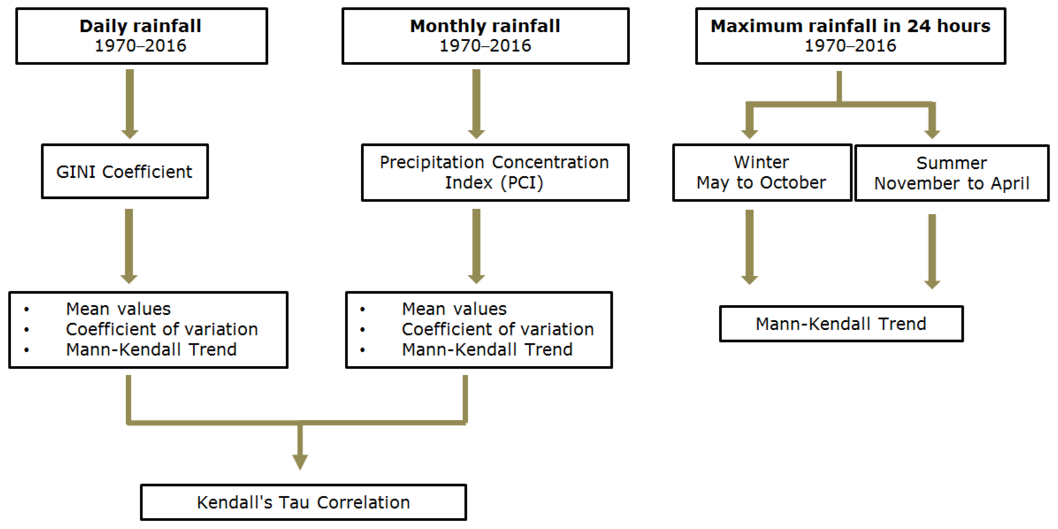
To analyze the concentration of daily precipitation in central Chile, the 1970–2016 period was considered (Figure 2). Rainfall records belong to the National Water Bank, managed by the General Water Directory of Chile (DGA), and to the Chilean Meteorological Directory (DMC). Both organizations (DGA and DMC) develop an exhaustive analysis of the quality of the obtained data, which are only available for scientific purposes, once the quality of the data has been validated.
Only stations having 45 or more years of records were considered. Although there are methods for filling in missing data that produce good results [42], it was preferred not to use them because of possible introduction of sample biases. Additionally, the Alexandersson’s homogeneity test [43] was applied to the annual rainfall records for all stations.
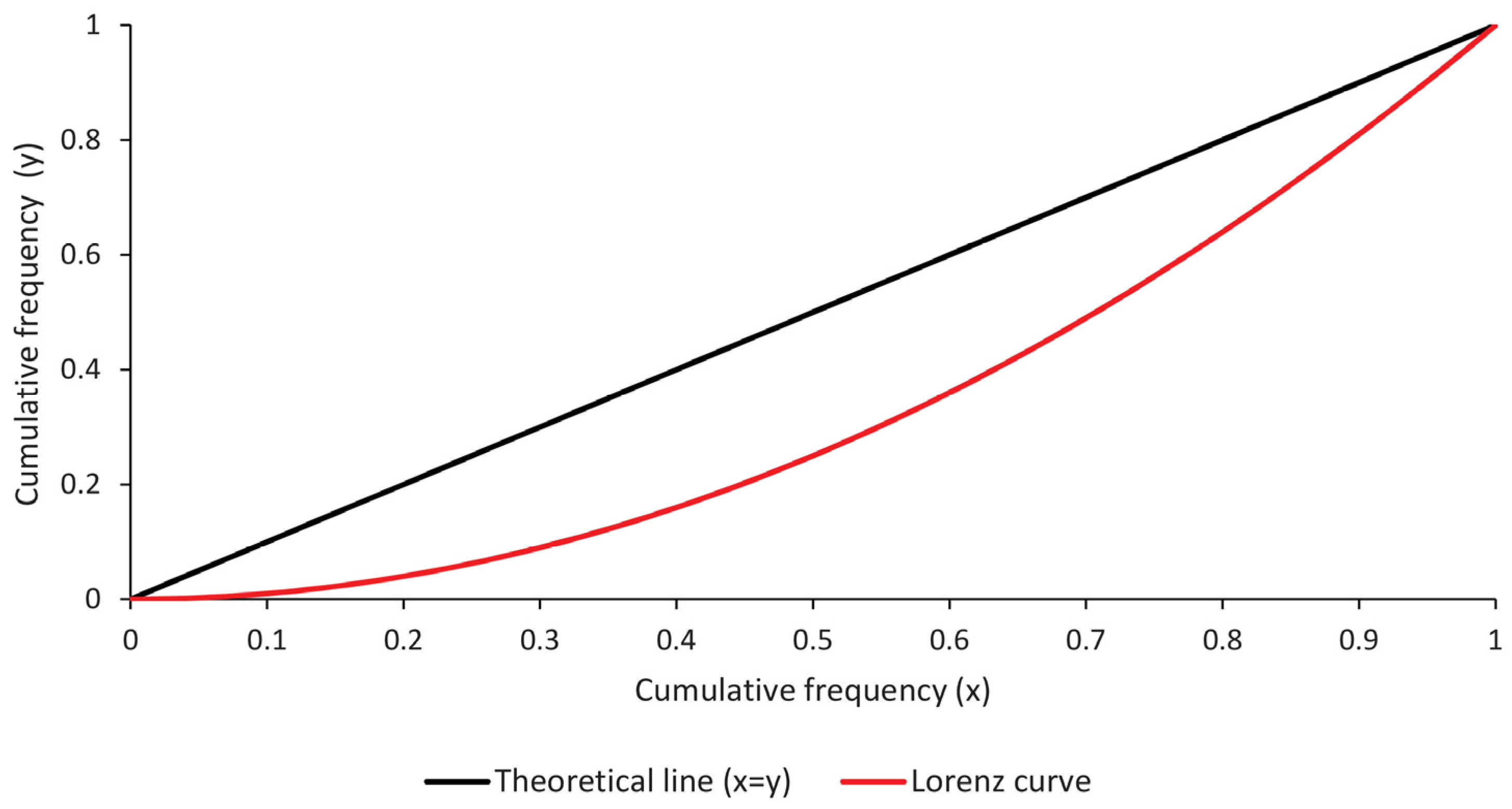
There are several methods for establishing precipitation concentration trends. In the field of hydrology, the rates of climatic aggressiveness have traditionally been used, but recently the Lorenz curve and the Gini index have been adopted from the field of econometrics. The Lorenz curve is a graphical representation of wealth concentration and indicates what percentage of accumulated wealth is in the possession of a given percentage of the population [44]. In ideal situations, the relationship between wealth and population is 1:1. The Gini Index originally estimates income inequality in the population and ranges between 0 and 1. When it is applied to daily rainfall, the value 1 indicates that a single day contributed to the yearly rainfall and the value 0 shows that yearly rainfall was uniformly distributed over the 365 days. Graphically, the Gini index is the ratio between the curve of perfect equity (y = x) and the Lorenz curve (y(x)), divided by the area under the equity curve (Figure 3).
The Gini index was applied in this study to daily rainfall values for each year, considering the 1970–2016 period and following the procedure by Yin et al. [23], who pointed out that the lack of precipitation is also an indicator for rainfall concentration. Thus, the Gini index is represented by the following expression, in which x and y are the cumulative proportions of the variables under study, and y(x) is the Lorenz curve
In addition, we worked with monthly precipitation values using the precipitation concentration index (PCI, Equation (2)), which explains the level of precipitation concentration during a given year [24]. Oliver [24] established that the value of this index fluctuates from 8.33% if rainfall is the same in all months, to 100% if all rainfall is concentrated in a single month. In other words, this index indicates whether rainfall in the rainy season is concentrated over a short or longer period of the year [45]. According to Oliver [24], the ranges for the PCI are the following: less than 10 suggests uniform distribution; between 11 and 20 denotes seasonal distribution; above 20 represents marked seasonal differences, with higher values being an indication of increasing monthly concentration.
where is the precipitation concentration index for year j, expressed as percent; is the precipitation of month i in the year j; and is the annual precipitation in the year j.
Additionally, the mean values for each rain gauge of the Gini index, PCI, and annual precipitation were correlated using the Kendall’s tau coefficient. One of the advantages of this test is that it does not assume normality in the distribution of the data, making it advantageous to be used with hydro-meteorological variables. The values obtained from the test range between 1 and −1, and values above/below ± 0.7 indicate strong correlations between the variables [46]. The Kendall’s tau coefficient, , is calculated as
where C and D are the concordant and discordant pairs values, Tx and Ty are the ties between the variables x and y, and n is the sample size.
Finally, temporal trends for maximum rainfall in 24 h at each of the 89 analyzed stations were evaluated. Maximum rainfall in 24 h was stratified in two periods, winter and summer, considering the period between April and September as winter, and between October and March as summer.
Temporal trends of the Gini index and PCI values were estimated for the entire 1970–2016 period and for each rain gauge. These trends were evaluated using the Mann–Kendall’s non-parametric statistical test, which detects trends in time series and is widely used in the analysis of hydro-meteorological variables [47]. One of its advantages is that it does not require for data to be normally distributed [48]. To calculate it, this test first requires the Kendall’s S statistic and its variance VAR(S). With these values, a standardized Z statistic is obtained when the sample size is greater than or equal to 8 [49], whose sign and value will determine the orientation and significance of the trend, respectively. For the S statistic, we use the expression
where the function sign(xj − xk) has the value 1 if xj − xk > 0; value 0 if xj − xk = 0; and value −1 if xj − xk < 0, and where xj and xk are consecutive values of the variable under study.
Next, the variance VAR(S) is defined as
Finally, with both values, the Z value is calculated depending on the result of S
All statistical analyses were done considering a 5% error.
3. Results
The Alexandersson’s test revealed that, out of the 89 analyzed stations, 94.4% of them were homogeneous; as a consequence, the whole sample was accepted for the analysis. Figure 4 shows the Lorenz curve for the Monte Grande station in the arid–semiarid zone, with a high concentration (the Gini Index value is almost 1) and the Maquehue Temuco station in the humid–subhumid zone, with a lower concentration of precipitation, both for 2016.
As shown in Figure 5, the Gini index is high in the arid–semiarid zone (higher concentration of precipitation) and decreases for stations as one moves towards the humid–subhumid zone (lower concentration of precipitation). When averaging the values of the Gini index in the studied period, it was observed that there was a low dispersion in both zones. However, the arid–semiarid zone normally presents a high concentration of precipitation, while the humid–subhumid zone has a greater variability in such variable, which was reflected by the Gini index.
In terms of the PCI, it is shown that as one moves latitudinally from the arid–semiarid zone, the values of this indicator tend to decrease by up to 30 percentage points in humid–subhumid zone stations. In fact, it was observed that in the arid–semiarid zone the PCI reached a value of 33.6%, whereas in the humid–subhumid zone it was remarkably reduced to 16.4%. This accounts for the great difference that exists between one zone and another, where the values of this indicator fluctuated between 20.7% and 58.6% in the arid–semiarid zone, and between 13.3% and 19.6% in the humid–subhumid zone. For the Gini index, calculated with daily data, it was determined that the index decreases almost two-tenths when moving from north to south, but increasing its coefficient of variation (CV) by three percentage points (Figure 5), with CV values fluctuating between 0.91 and 0.99 in the arid-semi-arid zone, and between 0.79 and 0.91 in the humid–subhumid zone. The Gini index uses daily data, and therefore includes days when there is zero precipitation, which is more frequent in the arid–semiarid zone than in the arid–semiarid zone. Both indices decrease their value as we advance from the arid–semiarid zone (29°12′S to 39°30′ S) to the humid–subhumid (34°44′ S to 39°30′ S) zone, denoting a lower concentration of precipitation at a monthly scale (PCI) and a daily (Gini) scale in the latter zone. Pizarro et al. [25] and Sarricolea & Martin-Vide [27] found similar relationships of higher concentration of rainfall towards the arid–semiarid zone, and decreases toward the south. However, Sarricolea et al. [28] did not find differences in the north-south gradient for the calculated IC values, for 16 stations located in a smaller territory (between 32°50′ S and 34°12′ S), compared to this study. As an example, Figure 6 shows the series of annual values of both indices for two stations in each zone, where their inter-annual variability is observed.
Figure 7 shows the PCI, GI, and precipitation behaviors, as well as the relationship among them. A clear difference is highlighted by the values of precipitation and their relationships with PCI and GI, comparing both climatic zones, corroborating the separation made between them.
When relating the Gini index to average annual precipitation (Figure 7c), it was observed that in the arid–semiarid zone there is a decrease in the value of this coefficient as average annual precipitation increases, in a range of low values. With respect to the humid–subhumid zone, a decrease in the Gini index value is also indicated as precipitation increases, but in a wider range than in the arid–semiarid zone. This is due to the fact that since there is more precipitation, a greater number of days with rainfall occurs (Figure 8), increasing the ‘equity’ of precipitation as the Gini index decreases. As the amounts of precipitation in the arid–semiarid zone are low (generally less than 350 mm per year), the variation of the index in that zone is minimal, at the level of 4-to-5 hundredths (0.91–0.99). In the humid–subhumid zone, on the other hand, the variation of the Gini index is more accentuated (15 hundredths) towards a greater equity in the concentration of precipitation, derived from rainfall amounts that reach up to the annual means of 3200 mm.
With respect to the relationship between PCI and the mean annual precipitation, Figure 7e shows that for the arid–semiarid zone, PCI decreases 33 percent as precipitation increases. The same happens in the humid–subhumid zone, but this decrease is not so pronounced (slightly higher than 10 decimal points). The above suggests that as precipitation increases in the arid–semiarid zone, there is a decrease in the concentration of precipitation. However, in the humid–subhumid zone, the decrease in the PCI as a function of the increase in precipitation is not so noticeable, since in this zone precipitation is notably more abundant and, therefore, the normal concentration is relatively low in relation to the arid–semiarid zone.
Comparing the average annual values of the Gini index, the average annual PCI, and the average annual precipitation using the Kendall’s tau coefficient, a strong correlation was observed between the average Gini value and the PCI for the two studied areas, with 0.91 and 0.86, respectively (Table 1). The above suggests that the pattern of precipitation concentration in the country is described in the same way by both the daily and monthly resolution, since both indices have similar behaviors. As for the relationship of both indices (Gini and PCI) with the average annual precipitation, it was observed that in the arid–semiarid zone the correlation is strong and inversely proportional, with values of −0.83 and −0.74, respectively, while in the humid–subhumid zone the correlations decrease to −0.41 and −0.32, respectively, although it remains inversely proportional.
Regarding the temporal behavior of the Gini index and the precipitation concentration index, for the 1970–2016 period the Mann–Kendall trend analysis shows that the Gini index in the arid–semiarid zone presents mostly positive trends (59.1% of stations), although only one of these was significant (Figure 9 and Figure 10). In the same area, 38.6% of stations showed negative tendencies, although only one of them was significant. A small proportion of significant trends can be observed, which allows us to state that there are no major changes in the precipitation concentration in this macro-zone over time.
When analyzing the humid–subhumid zone, it can be seen that trends are predominantly positive (91.1% of stations); however, significant trends are not most frequent, although they explain an important proportion (35.6% of stations) of the results. Values obtained in the humid zone indicate that annual precipitation is concentrating on fewer days. This concentration of precipitation could be explained by the changes in Chile’s climate regime since the 1970s [50].
On the other hand, the PCI showed that the ratio between positive and negative trends for both areas under study is lower than the Gini index (in the PCI, positive and negative trends are almost 1:1, while for the Gini index the ratio is 3:1). This difference would be a function of the nature of both indices, as the PCI uses monthly precipitation data and Gini index uses daily data, and hence has many zero values, which would be ignored when estimating monthly values. These values create a Lorenz curve with very little accentuation, so the Gini values are closer to 1. This same reason would also explain why there is little fluctuation in the Gini index at the arid–semiarid zone, since in this area the seasons are relatively long, with almost no precipitation. This difference in the data’s time scale was also found by Valdés-Pineda et al. [15], who analyzed seasonal trends (SR) of precipitations between 35° S and 40° S (humid–subhumid zone), finding negative trends in autumn and positive trends in winter.
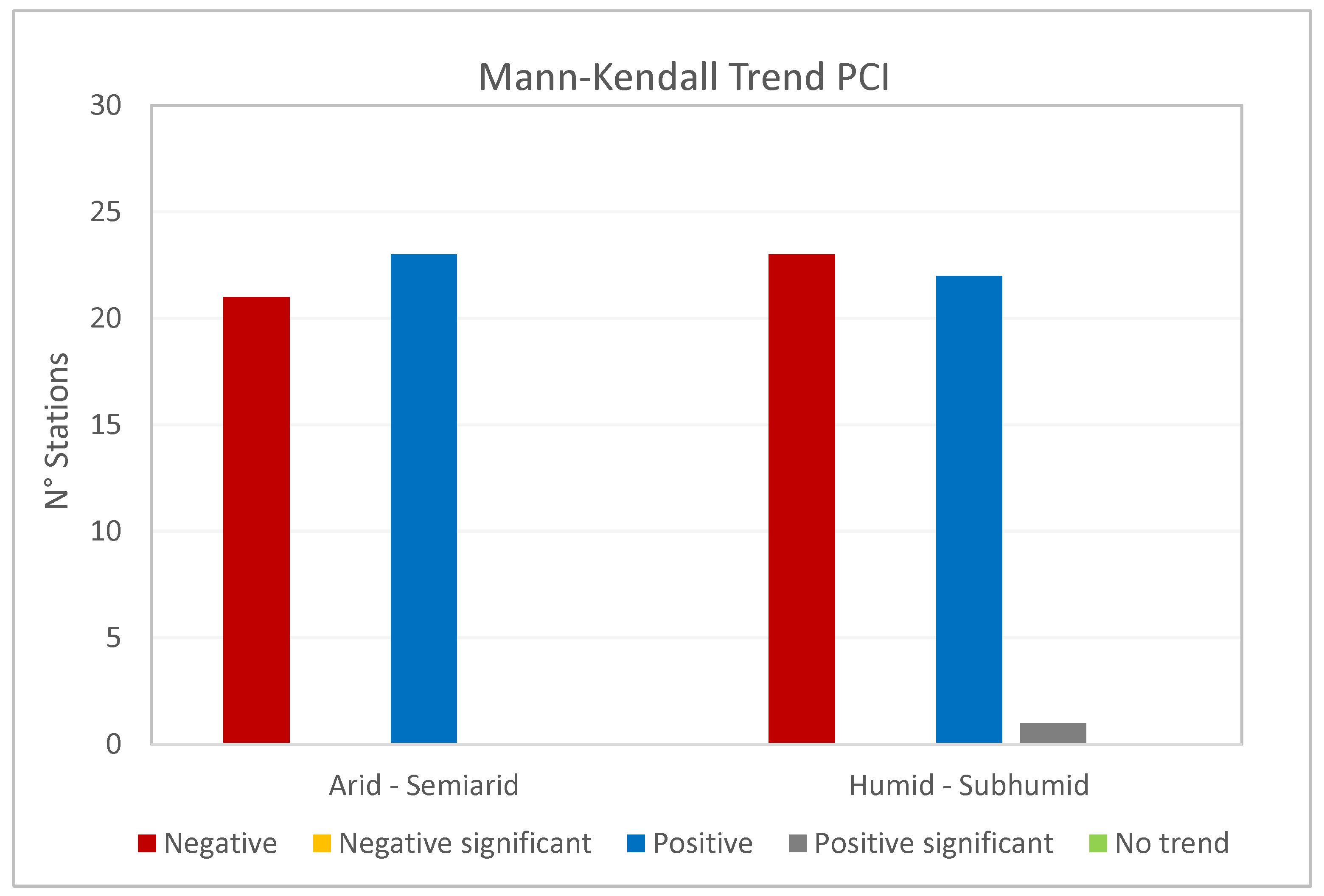
Analyzing the PCI trends (Figure 11), it can be seen that there is no greater difference between the two climatic areas under study. In the arid-semi-arid zone, 21 stations showed negative trends and 23 stations had positive trends, while in the humid–subhumid zone the situation is inverted, with 23 stations having negative trends against 22 with positive trends.
Analyzing trends in maximum precipitation over 24 h, separating them into summer and winter periods (Table 2), it was observed that in the arid–semiarid zone, and for both periods, the negative and positive trends are similar, although those with statistical significance are very small, not exceeding 1.5%.
The humid–subhumid zone shows greater number of negative trends for both periods (at least 30 percent points), and there is a higher statistical significance than in the arid–semiarid zone, especially in the case of negative trends, which rise to 10%.
4. Conclusions
As expected, obtained results indicate that precipitation concentration decreases as one moves from north to south; i.e., precipitation concentration is higher on both, daily and monthly scales in the arid–semiarid zone, compared to the humid–subhumid zone.
The Gini index and the PCI are positively correlated in both climatic zones, suggesting that both areas are relevant despite of their differences in the data’s temporal resolution. The Gini index determined that there is a predominance of positive trends in both areas, with a greater proportion in the humid–subhumid area, an indication that there is an increase in the concentration of rainfall, Although generally speaking there was no significance for the Gini Index, the humid–subhumid zone showed greater prevalence of positive trends, with statistical significances that was not negligible, an indication that rainfall is becoming more concentrated at the daily level in the humid–subhumid zone, not being the case for the arid–semiarid zone.
Both climatic zones show similar positive and negative trends for the PCI, allowing to conclude that annual rainfall concentration has remained relatively stable in both regions. Results obtained for the PCI in both areas under study suggest that, on an annual scale, there is no evidence of increases or decreases in the concentration of annual precipitations over time.
Finally, obtained results in the analysis of maximum precipitation trends over a 24-h period indicate that there were no major changes in maximum precipitation in the arid–semiarid zone. Likewise, there was a decrease of maximum precipitation in 24 h for the same period in the humid–subhumid zone, although with low statistical significance. This makes it possible to conclude that there is no clear evidence of a change in maximum precipitation over the last 47 years in both areas.
Acknowledgments
The authors of this study sincerely thank the Technological Center of Environmental Hydrology (University of Talca), the Faculty of Agricultural Engineering’s Department of Water Resources (University of Concepción), and the Faculty of Forest Sciences and Nature Conservancy (University of Chile). This study was partially funded by project CONICYT/FONDAP-15130015. This research is part of project FONDECYT 1160656.
Author Contributions
Claudia Sangüesa and Alfredo Ibañez processed the data gathered; Claudia Sangüesa and Roberto Pizarro analyzed the results and write the paper; Diego Rivera, Alfredo Ibañez, and Juan Pino made the plots; Diego Rivera, Pablo García-Chevesich, and Benjamin Ingram provided their insight and expertise in the analysis of the results and helped editing the paper; Juan Pino helped to analyze the results and write the paper.
Conflicts of Interest
The authors declare no conflict of interest. The founding sponsors had no role in the design of the study; in the collection, analyses, or interpretation of data; in the writing of the manuscript, and in the decision to publish the results.
References
- Puertas, O.; Carvajal, Y.; Quintero, M. Estudio de tendencias de la precipitación mensual en la cuenca Alta-Media del Río Cauca, Colombia. Dyna 2011, 78, 112–120. [Google Scholar]
- Intergovernmental Panel on Climate Change (IPCC). Contribution of Working Groups I, II and III to the Fifth Assessment Report of the Intergovernmental Panel on Climate Change; Pachauri, R.K., Meyer, L.A., Eds.; Climate Change 2014: Synthesis Report; IPCC: Geneva, Switzerland; p. 151.
- Singh, D.; Tsiang, M.; Rajaratnam, B.; Diffenbaugh, N.S. Precipitation extremes over the continental United States in a transient, high-resolution, ensemble climate model experiment. J. Geophys. Res. Atmos. 2013, 118, 7063–7086. [Google Scholar] [CrossRef]
- Zubieta, R.; Saavedra, M. Distribución espacial del índice de concentración de precipitación diaria en los Andes centrales peruanos: Valle del río Mantaro. Tecnia 2009, 19, 13–22. (In Spanish) [Google Scholar] [CrossRef]
- Pizarro, R.; Valdés, R.; García-Chevesich, P.; Vallejos, O.; Sangüesa, C.; Morales, C.; Balocchi, F.; Abarza, A.; Fuentes, R. Latitudinal analysis of rainfall intensity and mean anual precipitation in Chile. Chil. J. Agric. Res. 2012, 72, 252–261. [Google Scholar] [CrossRef]
- Organización de las Naciones Unidas para la Educación, la Ciencia y la Cultura (UNESCO). Documento País “Análisis de Riesgos de Desastres en Chile 2010”. VI Plan de Acción Dirección General de Ayuda Humanitaria y Protección Civil (DIPECHO) en Sudamérica. Available online: http://dipecholac.net/docs/files/315-documento-pais-chile-2010.pdf (accessed on 14 November 2011). (In Spanish).
- Garreaud, R. Cambio Climático: Bases Físicas e Impactos en Chile. Available online: http://dgf.uchile.cl/rene/PUBS/inia_RGS_final.pdf (accessed on 14 November 2011). (In Spanish).
- Montecinos, A.; Díaz, A.; Aceituno, P. Seasonal diagnostic and predictability of rainfall in subtropical South America based on tropical Pacific SST. J. Clim. 2000, 13, 746–758. [Google Scholar] [CrossRef]
- Gonzáles, A. Ocurrencia de eventos de sequías en la ciudad de Santiago de Chile desde mediados del siglo XIX. Revista de geografía Norte Grande 2016, 64, 21–32. [Google Scholar] [CrossRef]
- Ortlieb, L. Las mayors precipitaciones históricas en Chile central y la cronología de eventos ENOS en los siglos XVI-XIX. Rev. Chil. Hist. Nat. 1994, 67, 463–485. [Google Scholar]
- Escobar, F.; Aceituno, P. Influencia del fenómeno ENSO sobre la precipitación nival en el sector Andino de Chile central durante el invierno. Bulletin de L’institut Français D’études Andines 1998, 27, 753–759. (In Spanish) [Google Scholar]
- González, A.; Muñoz, A. Cambios en la precipitación de la ciudad de Valdivia (Chile) durante los últimos 150 años. Bosque 2013, 34, 191–200. [Google Scholar] [CrossRef]
- Acosta-Jamett, G.; Gutiérrez, J.; Kelt, D.; Meserve, P.; Previtali, M. El Niño Southern Oscillation drives conflict between wild carnivores and livestock farmers in a semiarid area in Chile. J. Arid Environ. 2016, 126, 76–80. [Google Scholar] [CrossRef]
- González-Reyes, Á.; McPhee, J.; Christie, D.; Le Quesne, C.; Szejner, P.; Masiokas, M.; Crespo, S. Spatiotemporal Variations in Hydroclimate across the Mediterranean Andes (30°–37° S) since the Early Twentieth Century. J. Hydrometeorol. 2017, 18, 1929–1942. [Google Scholar] [CrossRef]
- Valdés-Pineda, R.; Valdés, J.; Diaz, H.; Pizarro, R. Analysis of spatio-temporal changes in annual and seasonal precipitation variability in South America-Chile and related ocean–atmosphere circulation patterns. Int. J. Climatol. 2013, 36, 2979–3001. [Google Scholar] [CrossRef]
- Barrett, B.S.; Garreaud, R.D.; Falvey, M. Effect of the Andes Cordillera on Precipitation from a Midlatitude Cold Front. Mon. Weather Rev. 2009, 137, 3092–3109. [Google Scholar] [CrossRef]
- Montecinos, A.; Kurgansky, M.V.; Muñoz, C.; Takahashi, K. Non-ENSO interannual rainfall variability in central Chile during austral winter. Theor. Appl. Climatol. 2011, 106, 557–568. [Google Scholar] [CrossRef]
- Organización de las Naciones Unidas para la Educación, la Ciencia y la Cultura (UNESCO). Documento País “Análisis de Riesgos de Desastres en Chile 2012”. VII Plan de Acción Dirección General de Ayuda Humanitaria y Protección Civil (DIPECHO) en Sudamérica 2011–2012. Available online: http://www.unesco.org/fileadmin/MULTIMEDIA/FIELD/Santiago/pdf/Analisis-de-riesgos-de-desastres-en-Chile.pdf (accessed on 14 November 2011).
- Favier, V.; Falvey, M.; Rabatel, A.; Praderio, E.; López, D. Interpreting discrepancies between discharge and precipitation in high-altitude area of Chile’s Norte Chico region (26–32° S). Water Resour. Res. 2009, 45, W02424. [Google Scholar] [CrossRef]
- Sarricolea, P.; Romero, H. Variabilidad y cambios climáticos observados y esperados en el Altiplano del norte de Chile. Revista de geografía Norte Grande 2015, 62, 169–183. [Google Scholar] [CrossRef]
- Rubio-Álvarez, E.; McPhee, J. Patterns of spatial and temporal variability in streamflow records in south central Chile in the period 1952–2003. Water Resour. Res. 2010, 46, W05514. [Google Scholar] [CrossRef]
- Monjo, R.; Martin-Vide, J. Daily precipitation concentration around the world according to several indices. Int. J. Climatol. 2016, 36, 3828–3838. [Google Scholar] [CrossRef]
- Yin, Y.; Xu, C.-Y.; Chen, H.; Li, L.; Xu, H.; Li, H.; Jain, S. Trend and concentration characteristics of precipitation and related climatic teleconnections from 1982 to 2010 in the Beas River basin, India. Glob. Planet. Chang. 2016, 145, 116–129. [Google Scholar] [CrossRef]
- Oliver, J. Monthly precipitation distribution: A comparative index. Prof. Geogr. 1980, 32, 300–309. [Google Scholar] [CrossRef]
- Pizarro, R.; Cornejo, F.; González, C.; Macaya, K.; Morales, C. Análisis del comportamiento y agresividad de las precipitaciones en la zona central de Chile. Ingeniería hidráulica en México 2008, 23, 91–110. (In Spanish) [Google Scholar]
- Martín-Vide, J. Spatial distribution of a daily precipitation concentration index in peninsular Spain. Int. J. Climatol. 2004, 24, 959–971. [Google Scholar] [CrossRef]
- Sarricolea, P.; Martin-Vide, J. Distribución Espacial de las Precipitaciones en Chile Mediante el Índice de Concentración a Resolución de 1 mm, Entre 1965–2005; Climático, C., Impacto, E., Eds.; Spanish Climatology Association: Salamanca, Spain, 2012; pp. 631–639. (In Spanish) [Google Scholar]
- Sarricolea, P.; Herrera, M.; Araya, C. Análisis de la concentración diaria de las precipitaciones en Chile central y su relación con la componente zonal (subtropicalidad) y meridiana (orográfica). Investig. Geogr. Chile 2013, 45, 37–50. [Google Scholar] [CrossRef]
- De Luis, J.; González-Hidalgo, M.; Brunneti, M.; Longares, A. Precipitation concentration changes in Spain 1946–2005. Nat. Hazards Earth Syst. Sci. 2011, 11, 1259–1265. [Google Scholar] [CrossRef] [Green Version]
- Li, X.; Jiang, F.; Li, L.; Wang, G. Spatial and temporal variability of precipitation concentration index, concentration degree and concentration period in Xinjiang, China. Int. J. Climatol. 2011, 31, 1679–1693. [Google Scholar] [CrossRef]
- Rajah, K.; O’Leary, T.; Turner, A.; Petrakis, G.; Leonard, M.; Westra, S. Changes to the temporal distribution of daily precipitation. Geophys. Res. Lett. 2014, 31, 8887–8894. [Google Scholar] [CrossRef]
- Rojas, O.; Mardones, M.; Arumí, J.L.; Aguayo, M. Una revisión de inundaciones fluviales en Chile, período 1574–2012: Causas, recurrencia y efectos geográficos. Revista de geografía Norte Grande 2014, 57, 177–192. [Google Scholar] [CrossRef]
- Westra, S.; Alexander, L.; Zwiers, F. Global Increasing Trends in Annual Maximum Daily Precipitation. J. Clim. 2013, 26, 3904–3918. [Google Scholar] [CrossRef]
- O’Gorman, P. Precipitation extremes under climate change. Curr. Clim. Chang. Rep. 2015, 1, 49–59. [Google Scholar] [CrossRef] [PubMed]
- Asadieh, B.; Krakauer, N. Impacts of changes in precipitation amount and distribution on water resources studied using a model rainwater harvesting system. J. Am. Water. Resour. Assoc. 2016, 52, 1450–1471. [Google Scholar] [CrossRef]
- Organización de las Naciones Unidas para la Educación, la Ciencia y la Cultura (UNESCO). Atlas of Arid and Semi Arid Zones of Latin America and the Caribbean; Technical Documents of the UNESCO PHI-LAC, N25; UNESCO: Montevideo, Uruguay, 2010; ISBN 978-92-9089-164-2. [Google Scholar]
- Kottek, M.; Grieser, J.; Beck, C.; Rudolf, B.; Rubel, F. World map of the Köppen-Geiger classification updated. Meteorologische Zeitschrift 2006, 15, 259–263. [Google Scholar] [CrossRef]
- Peel, M.C.; Finlayson, B.L.; McMahon, T.A. Updated world map of the Köppen-Geiger climate classification. Hydrol. Earth Syst. Sci. 2007, 11, 1633–1644. [Google Scholar] [CrossRef]
- Spavorek, G.; De Jong, Q.; Dourado, D. Computer assisted Koeppen climate classification: A case study for Brazil. Int. J. Climatol. 2007, 27, 257–266. [Google Scholar] [CrossRef]
- Ministerio de Medio Ambiente y Medio Rural y Marino (MARM). Atlas Climático Ibérico; Agencia Estatal de Meteorología (Spain); Instituto de Meteorología de Portugal: Madrid, Spain, 2011; ISBN 978-7837-079-5.
- Kalvová, J.; Halenka, T.; Bezpalcová, K.; Nemešová, I. Köppen climate types in observed and simulated climates. Stud. Geophys. Geod. 2003, 47, 185–202. [Google Scholar] [CrossRef]
- Pizarro, R.; Ausensi, P.; León, L.; Aravena, D.; Sangüesa, C.; Balocchi, F. Evaluación de métodos hidrológicos para la completación de datos faltantes de precipitación en estaciones de la región del Maule, Chile. Aqua-LAC 2009, 1, 172–184. (In Spanish) [Google Scholar]
- Alexandersson, H. A homogeneity test applied to precipitation data. Int. J. Climatol. 1986, 6, 661–675. [Google Scholar] [CrossRef]
- Organización de las Naciones Unidas para la Alimentación y la agricultura (FAO). Inequality Analysis: The Gini Index; FAO: Roma, Italy, 2005. [Google Scholar]
- Schultz, R.E.; Maharaj, R.; Lynch, S.D.; Howe, B.J.; Melvil-Thomsam, B. African Atlas of Agrohydrology and Climatology. Section 4 Precipitation. 1997. Available online: http://www.iwmi.cgiar.org/pubs/working/wor76_sect2.pdf (accessed on 4 June 2007).
- Helsel, D.; Hirsch, R. Statistical Methods in Water Resources: Book 4, Chapter A3; U.S. Geological Survey: Reston, VA, USA, 1992.
- Ahmad, I.; Tang, D.; Wang, T.; Wang, M.; Wagan, B. Precipitation Trends over Time Using Mann-Kendall and Spearman’s rho Tests in Swat River Basin, Pakistan. Adv. Meteorol. 2015, 2015, 431860. [Google Scholar] [CrossRef]
- Song, X.; Song, S.; Sun, W.; Mu, X.; Wang, S.; Li, J.; Li, Y. Recent changes in extreme precipitation and drought over the Songhua River Basin, China, during 1960–2013. Atmos. Res. 2015, 157, 137–152. [Google Scholar] [CrossRef]
- Yue, S.; Pilon, P.; Cavadias, G. Power of the Mann-Kendall and Spearman’s rho tests for detecting monotonic trends in hydrological series. J. Hydrol. 2002, 259, 254–271. [Google Scholar] [CrossRef]
- Jacques-Coper, M.; Garreaud, R. Characterization of the 1970s climate shift in South America. Int. J. Climatol. 2015, 35, 2164–2179. [Google Scholar] [CrossRef]
Figure 1.
Study area and climate classification of Köppen–Geiger.
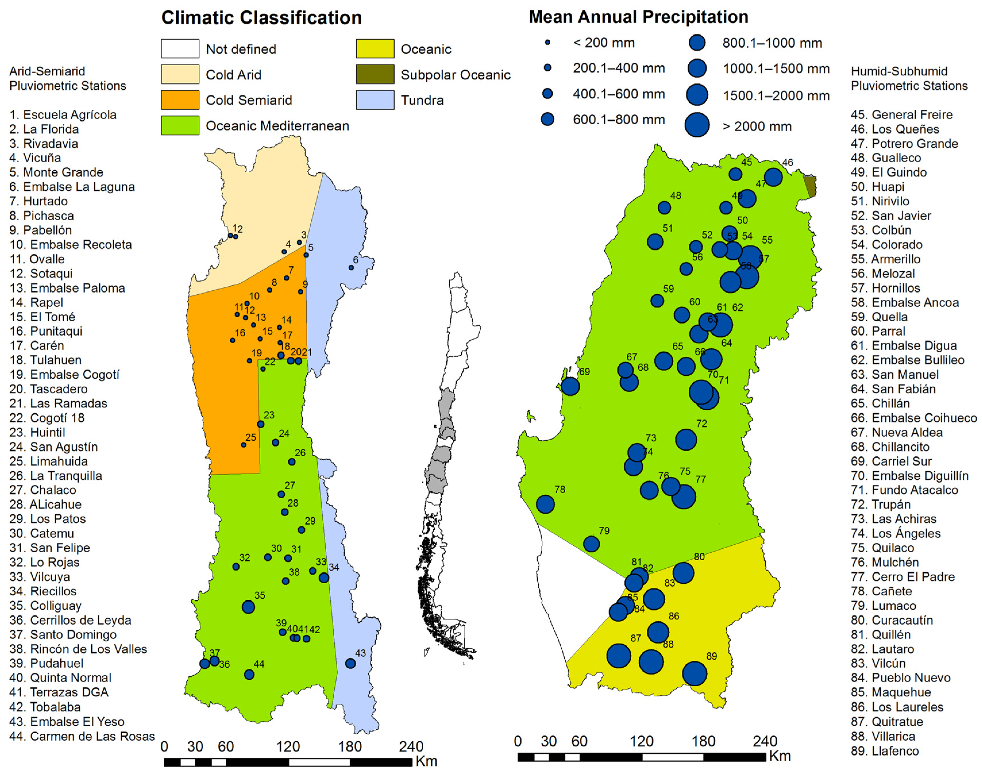
Figure 2.
Outline of the methodology.

Figure 3.
Graphical representation of the Gini index and the Lorenz curve.

Figure 4.
Lorenz curve for two pluviographic stations for the year 2016, in the study area. (a) Monte Grande pluviographic station; (b) Maquehue Temuco Ad pluviographic station.
Figure 4.
Lorenz curve for two pluviographic stations for the year 2016, in the study area. (a) Monte Grande pluviographic station; (b) Maquehue Temuco Ad pluviographic station.

Figure 5.
Results of the average value of the coefficients of Gini and PCI for the studied period (1970–2016) in the arid–semiarid and humid–subhumid zones.
Figure 5.
Results of the average value of the coefficients of Gini and PCI for the studied period (1970–2016) in the arid–semiarid and humid–subhumid zones.
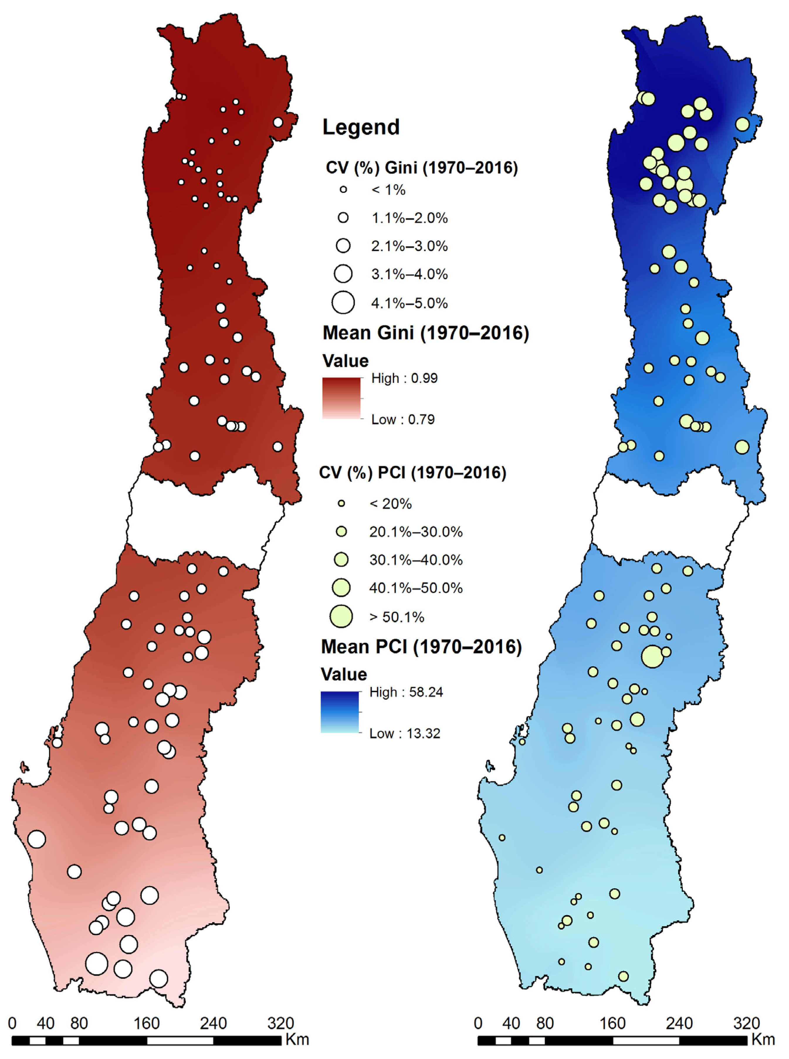
Figure 6.
Examples of annual PCI and Gini values for two stations located in the arid–semiarid zone, and two in the humid–subhumid zone. (a) Valores anuales de PCI para las estaciones Monte Grande y El Yeso Embalse en Arid-Semiarid zone; (b) Valores anuales de PCI para las estaciones Llafenco y Vilcún en Humid-subhumid zone; (c) Valores anuales de Gini Index para las estaciones Monte Grande y El Yeso Embalse en Arid-Semiarid zone; (d) Valores anuales de Gini Index para las estaciones Llafenco y Vilcún en Humid-subhumid zone.
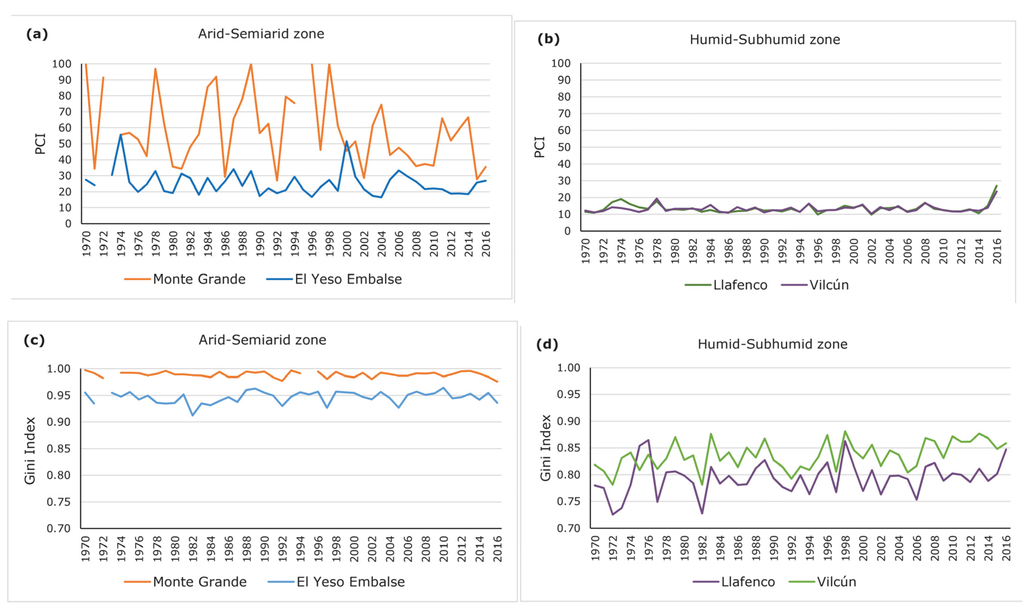
Figure 7.
Relationship between the mean Gini index (GI), PCI coefficient, and the mean annual precipitation (Pp) for each climatic zone in the period 1970–2016. The red boxes and circles indicate arid–semiarid zone and the black boxes and triangles indicate the humid–subhumid zone. The diagonal charts show the mean GI, PCI, and Pp values for each zone, while the rest of the charts illustrate the relationship among these parameters. (a)valores medios de Gini Index para Arid-Semiarid and Humid-Subhumid zones; (b) relación entre el Gini Index y el PCI; (c) relación entre Gini Index y precipitación; (d) valores medios de PCI para Arid-Semiarid and Humid-Subhumid zones; (e) relación entre el PCI y la precipitación; (f) valores medios de precipitación para Arid-Semiarid and Humid-Subhumid zones.
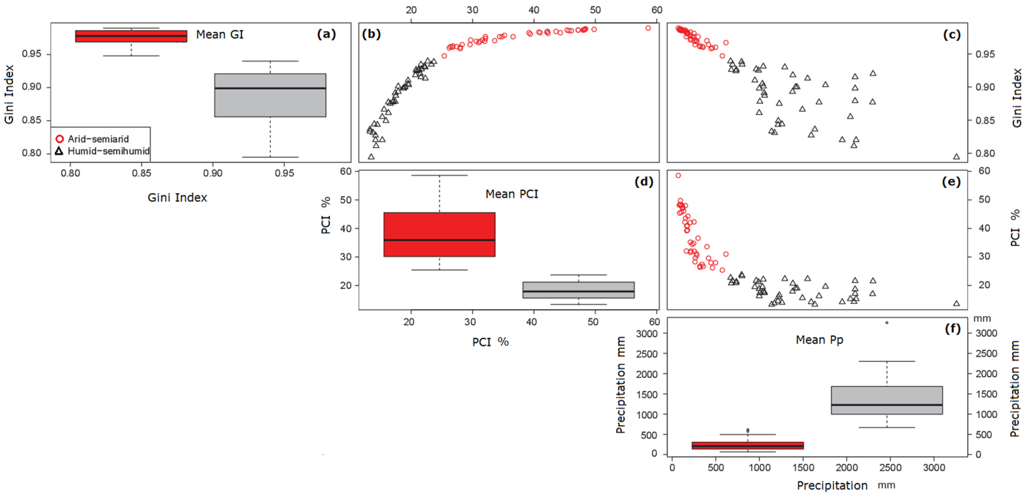
Figure 8.
Average annual number of rain-free days for the period analyzed.
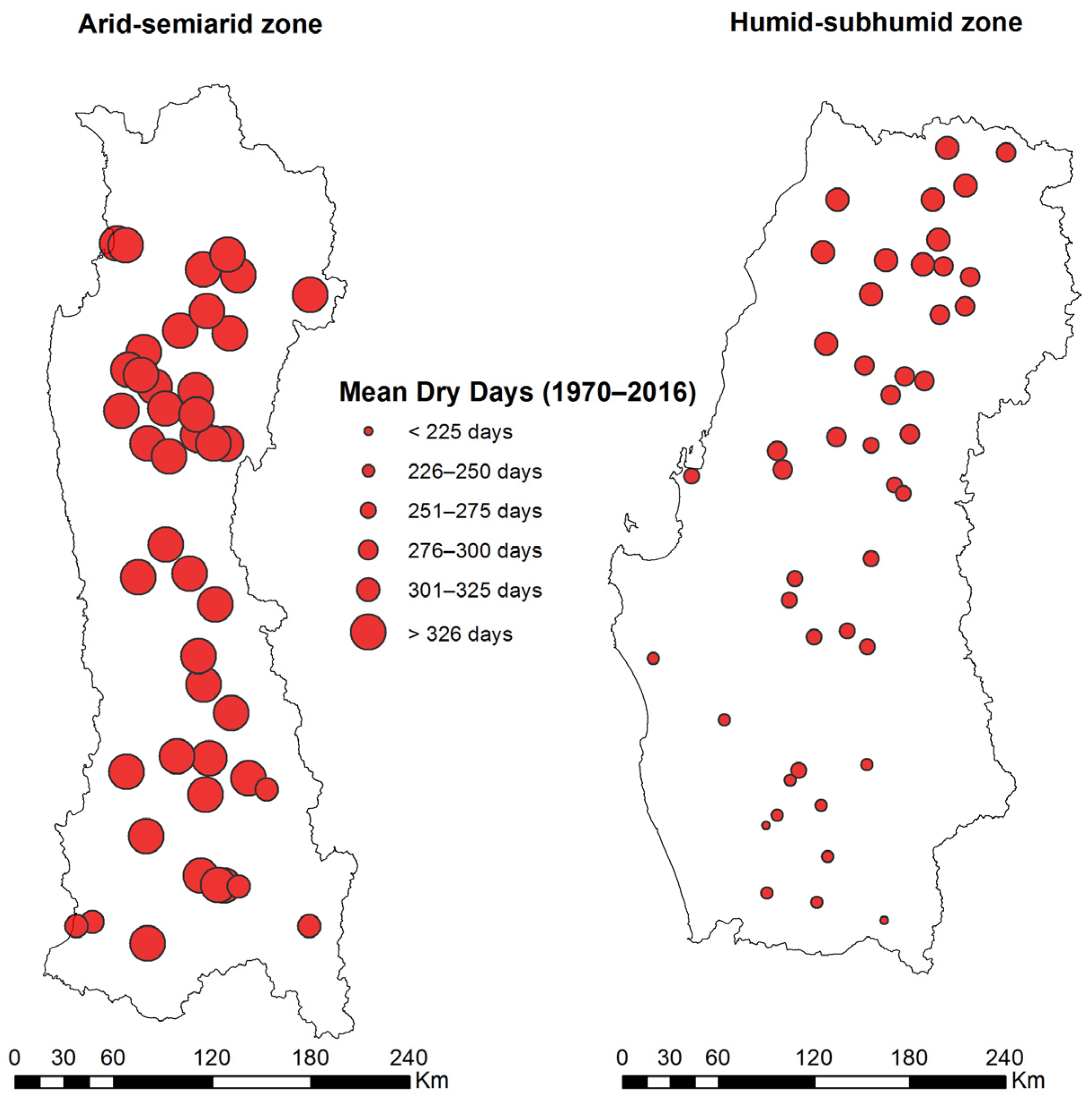
Figure 9.
Trends in the Gini and PCI coefficients based on the Mann–Kendall test.
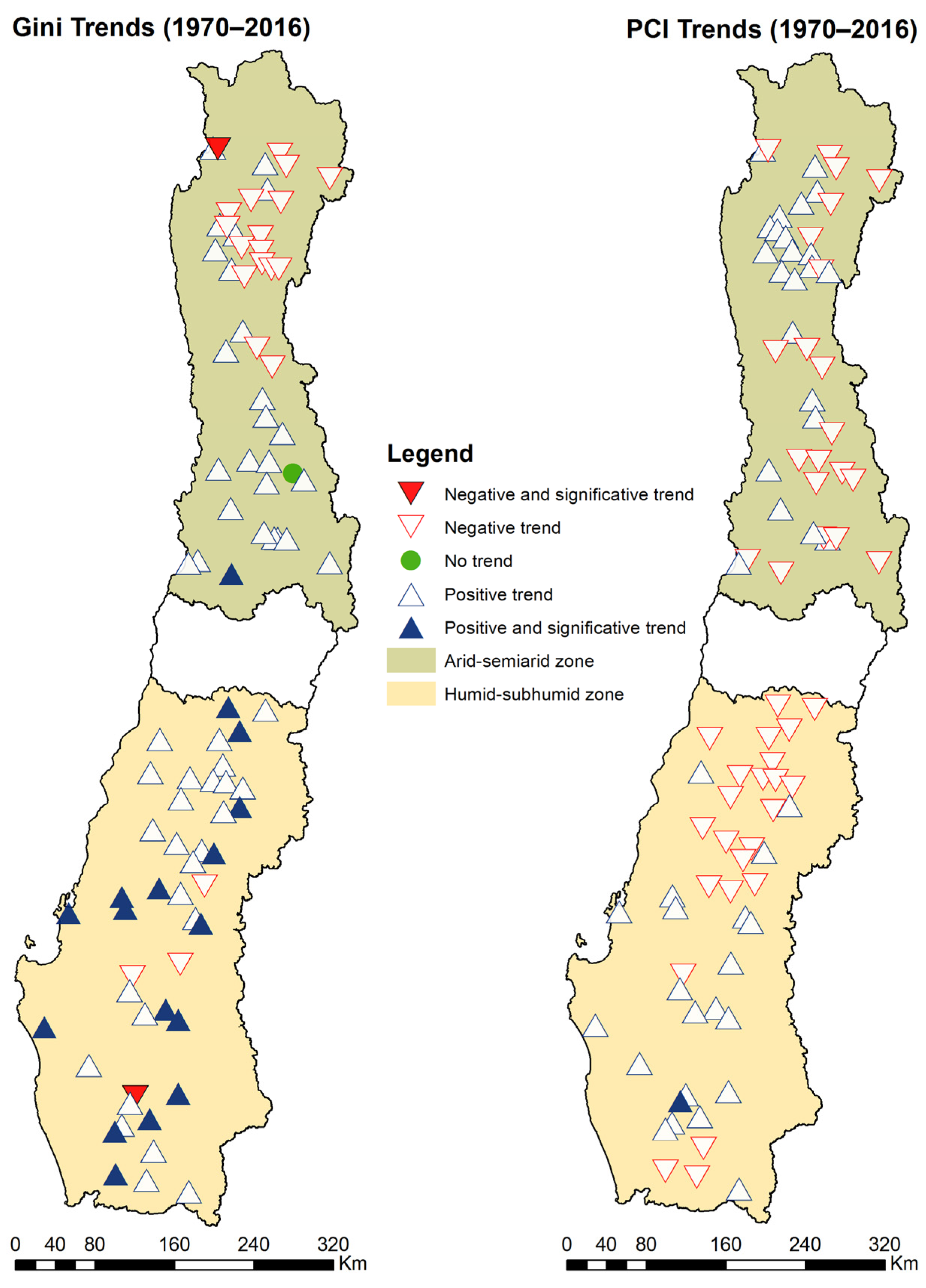
Figure 10.
Mann–Kendall trends found for the Gini coefficient.
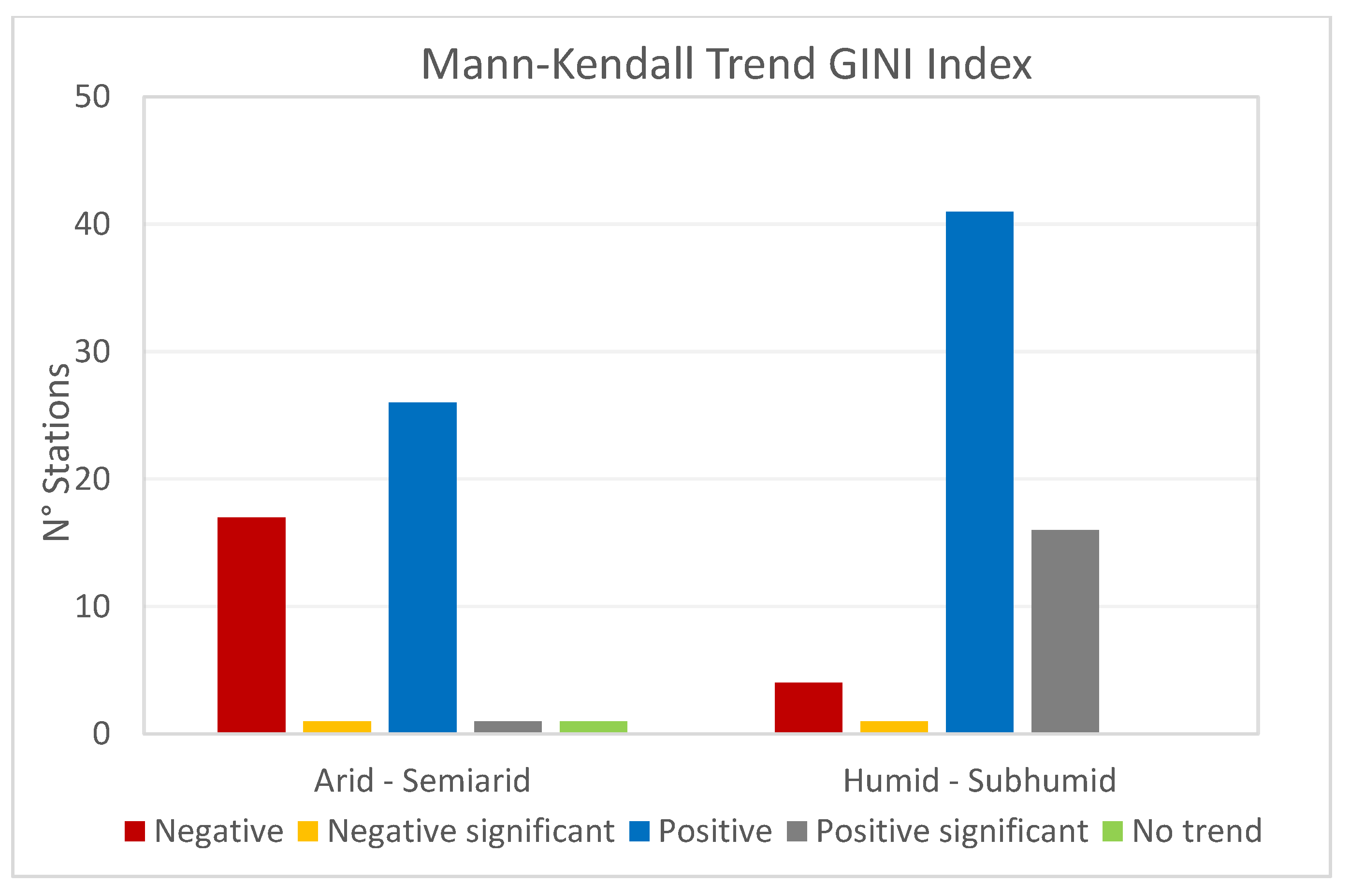
Figure 11.
Trends of the Mann–Kendall test in PCI for both zones.


Table 1.
Correlations (Kendall’s tau coefficient)
| Zone | Index | Gini | PCI | PP |
|---|---|---|---|---|
| Arid–semiarid | Gini | 0.91 * | −0.83 * | |
| PCI | 0.91 * | −0.74 * | ||
| PP | −0.83 * | −0.74 * | ||
| Humid–subhumid | Gini | 0.86 * | −0.41 * | |
| PCI | 0.86 * | −0.32 * | ||
| PP | −0.41 * | −0.32 * |
* p < 0.01.
Table 2.
Trends in 24-h maximum precipitation for each period (summer and winter)
| Zone | Period | Negative | Negative Significant | Positive | Positive Significant | No Trend |
|---|---|---|---|---|---|---|
| Arid–semiarid | summer | 140 (53.0%) | 1 (0.4%) | 114 (43.2%) | 4 (1.5%) | 10 (3.8%) |
| winter | 129 (48.9%) | 4 (1.5%) | 132 (50.0%) | 3 (1.1%) | 3 (1.1%) | |
| Humid–subhumid | summer | 210 (77.8%) | 9 (3.3%) | 57 (21.1%) | 0 (0%) | 3 (1.1%) |
| winter | 175 (64.8%) | 27 (10.0%) | 94 (34.8%) | 10 (3.7%) | 1 (0.4%) |
© 2018 by the authors. Licensee MDPI, Basel, Switzerland. This article is an open access article distributed under the terms and conditions of the Creative Commons Attribution (CC BY) license (http://creativecommons.org/licenses/by/4.0/).
Share and Cite
MDPI and ACS Style
Sangüesa, C.; Pizarro, R.; Ibañez, A.; Pino, J.; Rivera, D.; García-Chevesich, P.; Ingram, B. Spatial and Temporal Analysis of Rainfall Concentration Using the Gini Index and PCI. Water 2018, 10, 112. https://doi.org/10.3390/w10020112
AMA Style
Sangüesa C, Pizarro R, Ibañez A, Pino J, Rivera D, García-Chevesich P, Ingram B. Spatial and Temporal Analysis of Rainfall Concentration Using the Gini Index and PCI. Water. 2018; 10(2):112. https://doi.org/10.3390/w10020112
Chicago/Turabian StyleSangüesa, Claudia, Roberto Pizarro, Alfredo Ibañez, Juan Pino, Diego Rivera, Pablo García-Chevesich, and Ben Ingram. 2018. "Spatial and Temporal Analysis of Rainfall Concentration Using the Gini Index and PCI" Water 10, no. 2: 112. https://doi.org/10.3390/w10020112
Note that from the first issue of 2016, this journal uses article numbers instead of page numbers. See further details here.