Simulating Water Allocation and Cropping Decisions in Yemen’s Abyan Delta Spate Irrigation System

1
Department of Civil, Environmental & Geomatic Engineering, University College London, Gower Street, London WC1E 6BT, UK
2
National Forestry Commission, Periférico Poniente 5360, Col. San Juan de Ocotán, Zapopan, Jalisco 45019, México
3
School of Mechanical, Aerospace and Civil Engineering, The University of Manchester, Manchester M13 9PL, UK
*
Author to whom correspondence should be addressed.
Water 2018, 10(2), 121; https://doi.org/10.3390/w10020121
Submission received: 30 November 2017
/
Revised: 28 December 2017
/
Accepted: 26 January 2018
/
Published: 29 January 2018
(This article belongs to the Special Issue Hydroeconomic Analysis for Sustainable Water Management)
Abstract
:Agriculture employs more Yemenis than any other sector and spate irrigation is the largest source of irrigation water. Spate irrigation however is growing increasingly difficult to sustain in many areas due to water scarcity and unclear sharing of water amongst users. In some areas of Yemen, there are no institutionalised water allocation rules which can lead to water related disputes. Here, we propose a proof-of-concept model to evaluate the impacts of different water allocation patterns to assist in devising allocation rules. The integrated model links simple wadi flow, diversion, and soil moisture-yield simulators to a crop decision model to evaluate impacts of different water allocation rules and their possible implications on local agriculture using preliminary literature data. The crop choice model is an agricultural production model of irrigation command areas where the timing, irrigated area and crop mix is decided each month based on current conditions and expected allocations. The model is applied to Yemen’s Abyan Delta, which has the potential to be the most agriculturally productive region in the country. The water allocation scenarios analysed include upstream priority, downstream priority, equal priority (equal sharing of water shortages), and a user-defined mixed priority that gives precedence to different locations based on the season. Once water is distributed according to one of these allocation patterns, the model determines the profit-maximising plant date and crop selection for 18 irrigated command areas. This aims to estimate the impacts different water allocation strategies could have on livelihoods. Initial results show an equal priority allocation is the most equitable and efficient, with 8% more net benefits than an upstream scenario, 10% more net benefits than a downstream scenario, and 25% more net benefits than a mixed priority.
1. Introduction
Spate irrigation, the diversion of intermittent wadi flows in wet seasons, is practiced in 18 countries across the Middle East, North and East Africa, and West Asia [1]. With more than three million hectares of land under spate irrigation worldwide, many areas have grown dependent on this practice [1]. There is a high level of risk and unpredictability intrinsic to this practice as the exact timing and quantity of floods are unknown.
Middle Eastern countries reliant on spate irrigation often face a high level of risk as they also suffer from low per capita water availability [2]. For example, in much of Yemen’s rural areas, water availability is as low as 150 m3/capita/year [2]. When livelihoods are dependent on scarce supplies of irrigation water, conflicts over water use can arise. This is true of the Abyan Delta, one of Yemen’s largest irrigated areas with the potential to be the most agriculturally productive region in the country [3]. Water disputes have been linked to over 100 deaths in the Abyan Delta over the past decade, and to a number of other violent events throughout the country [4,5]. Despite the Abyan Delta receiving enough water to be the largest and most productive agricultural region in the country, 50% of the rural population still faces poverty [3,6]. The absence of clear water rights [2] combined with local resource inequalities has resulted in an unbalanced water allocation and much contention between influential upstream farmers and less privileged downstream users. According to a recent study, 70–80% of the conflicts which occur in Yemen’s rural areas are rooted in disagreements concerning water use [7].
Water allocation in spate irrigated systems can follow a wide range of approaches. Mehari, van Steenbergen and Schultz discuss a variety of rules for managing unpredictable flood waters within spate irrigated regions [1]. One strategy commonly practiced in lowland spate-irrigated areas in Eritrea, Yemen and Pakistan is to establish demarcation rules. Demarcation rules define boundary lines for the different areas entitled to irrigation. Each of these areas are then assigned a water allocation priority dependent on their year of establishment. This method tends to discourage new fields as they receive the lowest water allocation priority. Within the indigenous systems in Eritrea, flood water is divided using both proportional and rotational distributions. If the flow of a flood event is between 25 and 100 , the water is proportionally distributed to all the areas along that canal. If the flood event is less than 25 m3/s, then a rotational distribution is utilized. Ghebremariam and van Steenbergen discuss the water allocation practices of the Bada region of Eritrea, where landowners with flood water access follow several types of rules [8]. The most frequently used method, called Dinto, distributes water according to sequence rules. Aimed at reducing the inequity in water distribution, farmers are restricted from irrigating a second time until all fields have received an initial volume of irrigation water. When water is scarcest, an irrigation committee determines which fields should receive highest priority by considering soil moisture rather than location.
Various authors have built models of spate irrigation systems to determine how different allocation policies impact yields. The Spate Management Model (SMM) by El-Askari simulates practices within spate-irrigated areas of Yemen, then looks for areas of improvement in the operational or management procedures [9]. In SMM the user can set the water allocation priority of different irrigation command areas. Using predetermined cropping patterns for each command area the model can evaluate yields for each of the different allocation scenarios. Mehari et al. use a Soil Water Accounting Model (SWAM) to track soil moisture balance and yields within a spate irrigation system in Eritrea [10]. The model considers three hydrological scenarios. Each of the scenarios have a varying periodicity of irrigation and categorization of flood events, allowing the authors to assess how the timing and frequency of water allocation within the irrigation system impacts yields for sorghum and maize. Following the introduction of new hydraulic infrastructure, the authors recommended new allocation rules to more equitably and productively allocate water. Ward, Amer and Ziaee consider how the allocation of water impacts food security, although not in a spate irrigation context [11]. Their study identifies which water allocation rules minimise the loss in economic benefits and food security during water shortages. The analysis considered several water allocation rules including various upstream and downstream priorities and historical use patterns. Findings suggest a proportional sharing of water shortages, in which case each canal bears an equal proportion of overall shortages, was the best strategy for limiting threats to farm incomes.
To evaluate the impact of different water allocation rules on the spate irrigation system in Yemen’s Abyan Delta, our study proposes a linked simulation of water allocation, soil moisture and crop growth, and crop choice. The proposed integrated assessment model aims to simulate plausible agricultural decisions in order to evaluate policies, in this case water allocation scenarios.
The remaining sections of this paper discuss water management in the Abyan Delta to include existing infrastructure, agricultural practices, and historical context. This is followed by a description of each component of the integrated assessment model: water flow and allocation, soil-moisture and crop yield, and crop-selection modelling. The model’s application to the Abyan Delta spate irrigation system and its results are then described and discussed. A summary of model limitations and possible extensions is followed by conclusions.
2. Spate Irrigation and the Abyan Delta
The Abyan Delta is located in south Yemen near the Gulf of Aden. The population of Abyan is nearly half a million and is spread over eleven districts [12]. The annual rainfall is 235 mm with 69% of the rain occurring during June, July and August [13,14]. Wadi Bana, the main wadi of the Abyan Delta, had a mean annual inflow of 162 million . between 1951 and 1965 [15]. Two irrigation seasons account for nearly 90% of the annual runoff [15]. The Kharif season, the wettest season which occurs between 1 July and 15 October, receives 66% of annual runoff [15]. Another 24% arrives during the Seif season between 16 March and 31 May, with the remaining inflow volumes arriving during “off-season” months [15]. More up-to-date hydrological information was not available for this study.
The Abyan Delta has 40 thousand hectares of irrigable land [16]. The primary water source for irrigating the delta comes from spate irrigation, with the secondary source being groundwater [16]. These sources of water are not enough to meet the Abyan Delta’s full economic irrigation potential. Water shortages are not shared equitably across the system and this has led to or exacerbated violent local conflicts.
2.1. Agricultural System and Practices
Wadi Bana has five main weirs that function as irrigation diversion points (see Figure 1). The weirs are connected by a canal system, which allows distribution to all irrigated areas [17]. Within the Abyan Delta region, water is traditionally allocated to upstream fields first, with the constraint that they achieve only one “saturation irrigation” per season. Once the demand of upstream users is satisfied, the water is passed to those fields further downstream [18].
The main crops cultivated in the Abyan Delta are mango, watermelon, banana, papaya, lemon, cotton, sesame, groundnut, tomato, sorghum, millet, wheat, and maize [15,16,19]. Sorghum, millet, wheat, and maize are the main subsistence crops. Cash crops such as cotton or sesame are usually grown only after a staple crop has been harvested and a minimum annual income has been achieved [17]. Due to water shortages within the region, most crops are irrigated at only 80% of their water requirement or lower [16,20,21].
2.2. Water Management in the Abyan Delta
The history of the Abyan Delta is shaped by powerful regional tribes with the capacity to exert influence given the relative absence of a strong national government [22]. Throughout the 20th century, the Fadhli sultanate inhabited the southern half of the delta while the Yafa’e sultanate occupied the northern half. With Abyan water flowing north to south, the Yafa’e have historically been the first to divert and utilize wadi flood waters. This left the downstream Fadhli with water shortages during dry years, forcing them to grow fewer crops. As the two sultanates were in a constant conflict over this inequitable water distribution, the colonial administration of Great Britain initiated the Abyan Scheme, a project that modernised the existing irrigation scheme in 1938 as an attempt to resolve regional conflict [23]. Between 1947 and 1967, the Abyan Board managed the scheme which included responsibilities such as distributing irrigation water to different fields and prescribing the acreage to be allotted for different crops [24]. Control of the board was transferred from the British government to Yemen’s Ministry of Agriculture in 1967. After the 1994 civil war, the board lost power and could no longer enforce water distribution agreements. As a consequence, the farmers downstream resorted to groundwater extraction while the Yafa’e farmers upstream continued to irrigate their fields using water from Wadi Bana [4]. With groundwater volumes decreasing the Fadhli are again facing water shortages. This has once more highlighted the seemingly inequitable distribution of flood water within the Abyan Delta. An agreed upon set of water allocation rules could help reduce water conflict and enable more stable socio-economic development [4]. This study builds an integrated assessment framework linking three models aimed at evaluating different water allocation rules.
3. Methods
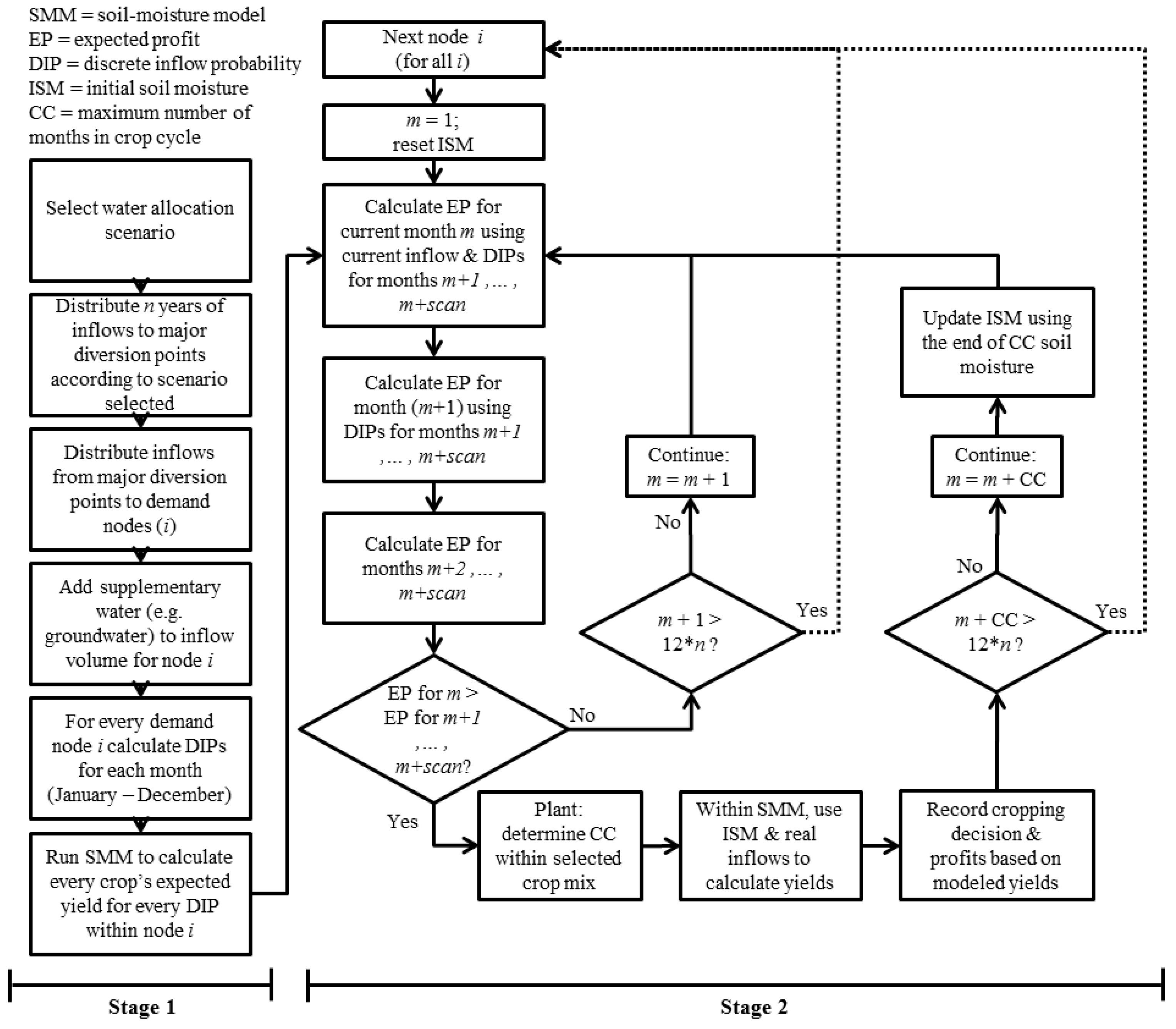
The motivation for an integrated assessment in situations such as the Abyan Delta is to help understand how the physics, agricultural production and resource management policies of the system are interdependent, and how changes could impact livelihoods [25]. The proposed agro-hydrological spate irrigation system integrated simulation model uses three linked sub-models: a water allocation simulator, a soil moisture and crop yield model, and a crop choice model. The first is a conventional optimisation-driven water allocation simulator which allows representing water sharing arrangements in a generic way [26]. The simulator allocates flood inflow volumes to the major diversion points (weirs in our case) based on analyst-defined distribution priorities. Water is then distributed amongst the individual irrigated “command areas” which are fed by canals leaving the major diversions. The soil moisture and crop yield model provides expected crop yields for each command area which follow from expected water allocations. Given the current and future expected allocations, a two-stage stochastic optimisation crop choice model determines the profit-maximising planting date, irrigated area, and the irrigable area each crop should be allotted. This sequence of events is depicted in Figure 2. Two of the three sub-models are optimisation models but they are not used in a prescriptive sense: their purpose is to simulate allocations and plausible farmer actions to evaluate how different allocation policies could impact agricultural production.
3.1. Water Flow and Allocation Modelling
The water distribution network consists of a surface water inflow point (with monthly inflows), major diversion points and irrigation “command areas”. Each month’s inflows are distributed amongst the major diversion points, represented by five weirs for the Abyan Delta case-study. Once monthly inflows are partitioned amongst the major diversions, the water is further distributed amongst those irrigation command areas that are connected to the major diversions. Diversions are modelled using a flexible linear-programme driven distribution model which adheres to the following set of constraint equations. Equation (1) is a generic network mass balance formula. As this model was designed for systems without surface water storage, Equation (2) prevents the supply for any node from exceeding its demand. Equation (3) mandates each allocation be non-negative.
For the above equations, is the wadi inflow at time-step t; . is the amount of water (Mm3) allocated to node i during time-step t; is the water loss between node i and the node closest upstream to node i; and is the annual water demand at node i.
We simulate different water allocation rules using either priority-penalties or overall deficit minimisation (equal priority). The priority allocation system is driven using:
where is the amount of water (M) allocated to node i during time-step t and is a priority weight for node i.
The order of water diversion priority is prescribed by giving each diversion point a priority weight (). This value is assigned by the modelers to reflect the allocation scenario being analysed. The equal priority approach minimises deviations from target allocations for all water demand nodes:
where is the demand (M) for node i and is the supply (M) for node i.
3.2. Soil-Moisture Modelling
Tracking soil moisture allows predicting crop yield values. The soil moisture balance in the proposed model considers the simulated water allocations as well as all simulated cropping decisions. To track soil moisture we use standard methods of the Food and Agriculture Organization (FAO), summarised in Appendix C [27]. To calculate the infiltration of water on bare soil, slight modifications were made to FAO’s AquaCrop methodology (Appendix C). Evapotranspiration of crops was calculated using the Penman–Monteith equation following FAO guidelines [28]. If no crops are selected, the model continues the soil moisture tracking without evapotranspiration. Specific inputs for this calculation are listed in Section 4.1. The water stress coefficients (Ks), crop actual evapotranspiration (ETc), total available water in the root zone (TAW), readily available soil moisture (RAW), soil moisture deficit, and actual yield were all calculated using the equations in Appendix C. Combining these models results in a soil moisture tracking model that estimates yields and profits for any crop mix.
3.3. Crop Selection Model Formulation
The crop choice model considers water allocations and attempts to emulate reasonable cropping decisions that could be made by a farmer under similar hydrological and agronomic circumstances. To accomplish this, the authors use a two-stage stochastic programme to determine the profit maximising plant date and selection of crops, as well as the amount of land each crop should be allotted. The objective function equation (Equation (6)) seeks to maximise net benefits by determining how much of each crop c should be grown in each month m. This calculation is made while adhering to constraints on land availability (Equation (7)), the current month’s available water supply (Equation (8)), and the anticipated water availability for each of the future months within the “scan” period, d (Equation (9)). The “scan” period is a number of future months a farmer will consider when making seasonal cropping decisions. The future water availability is represented in the objective function equation with k discrete inflow probabilities. The profit-maximising cropping decision is determined with an expected value of profit given inflow probabilities. The model considers every potential crop mix and finds the one with the greatest expected net benefits:
where is the probability of hydrologic event j (monthly); is the area allocated to crop c under condition j, within node i (ha); is the yield for crop c under condition j (kg/ha); is the profit of crop c (YR/ha); is the irrigable area in node i (ha); is the water requirement for crop c in month m (M/ha); is the water allocated to node i under condition j; is the monthly volume of groundwater available for node i (M); is the yield response factor; is the actual crop evapotranspiration (mm); is the crop evapotranspiration (mm); is the maximum yield (kg/ha); is the current month; and is the duration of the growing season.
When the crop selection with the highest expected profit has been identified, the expected value is used to determine the optimal amount of area to assign each crop (Equation (11)):
where is the area allocated to crop c within node i (ha); is the probability of hydrologic event j (monthly); and is the area allocated to crop c under condition j, within node i (ha).
3.4. Integrated Model
The model components are linked at run time to form an integrated model, as depicted in Figure 2 and described next.
The integrated model can be considered a subcommand area agent model, which attempts to predict plausible agricultural decisions farmers might make. For each command area (i), the integrated model considers expected profits of future months to choose when to plant. If the current month’s expected profit is largest, that crop mix becomes what is grown and a daily soil moisture balance is launched to estimate yields.
Using the water flow and allocation model (Section 3.1), each irrigated command area is allotted a volume of water per month. Once wadi inflows have been distributed, a monthly volume of supplementary water (e.g., groundwater) may be added to each command area. The model then generates a number of discrete inflow probabilities for each month and command area. Based on these discrete inflow probabilities, the expected yield for each crop is calculated within every command area. The expected yield of all growable crops is generated for each of the discrete inflow probabilities using the soil moisture model on a monoculture basis. This sequence of events is shown in “Stage 1” of the flow diagram above. Additional information on each of the growable crops may be found in Appendix D.
“Stage 2” of the integrated model tracks agricultural decisions over time for all command areas. Within this process, the model first determines the current month’s profit-maximising crop selection and expected profit (Section 3.3). This is calculated using the current inflow and discrete inflow probabilities for each future month within the “scan” period, under the constraint that the crop mix’s water requirements must be less than the current and expected future inflows. The scan period is a window of months during which a farmer compares expected profits and determines whether or not to plant in the current month. After calculating the current month’s expected profit, the model then determines the expected profit for each future month within the scan period. When analysing the expected profit for each of these future months the water availability consists of discrete inflow probabilities only.
If the current month has a higher expected profit than any future month within the scan period, the model infers it is sensible to plant in the current month. If not, the model assumes no planting in the current month and repeats the analysis for the following month. Once the model has chosen a planting time and crop selection the profit is calculated. Profit is different from expected profit as it considers how the selected crop mix will impact soil moisture and consequently the crop yields, as opposed to using expected yields based on the discrete inflow probabilities. Soil moisture is updated daily throughout the time-horizon, taking into consideration water allocations as well as all previous cropping decisions within the simulation. Once profit has been recorded the model reinitiates “Stage 2” of the integrated model, starting from the month when the previous crop selection completed its cycle. Initial conditions for the soil-moisture model are of bare soil with soil moisture at field capacity.
4. Application to the Abyan Delta
The Abyan Delta system architecture consists of five weirs, each with their respective set of command areas—totalling 18 command areas in all (Figure 1). Within Equations (1)–(5), nodes i through n refer to the five weirs. When water has been distributed to the weirs, it is then partitioned amongst the command areas using the same set of equations, with nodes i through n now representing the 18 command areas. For all other equations, the index i always corresponds to the 18 command areas. When running the crop-choice model, there are 33 crops which may be considered for selection. For all equations, these crops correspond to the index c. The “scan” period, d, was set at three months for application to the Abyan Delta. With the “scan” period set at three months, the modellers are able to replicate a farmer considering the best time to plant over a four-month period (m, m + 1, m + 2, m + 3). This allows for an analysis over the entirety of the two irrigation seasons—Kharif season which lasts 3.5 months and the Seif season which is 2.5 months. Lastly, 16 discrete inflow probabilities, j, were considered for this case-study.
4.1. Water Supply and Demand Data
Inputs for the water modelling include historical flow data from 1951 to 1965 (summarised in Figure 3) and annual water demands. The annual water demand for each weir determines the maximum water volume that weir can utilize per year. Again, because this model was designed to examine systems without surface water storage, the annual water demand per weir cannot be exceeded.
Referencing field work conducted by Atkins, the annual water demands for each of the five weirs are as follows: 62.9 for Bateis, 23.5 for Haiga, 26.3 for Diyyu, 23.8 for Makhzan, and 23.2 for Gharaib [15]. These demands were estimated using a 72 cm water-depth requirement for each of the fields receiving irrigation water from their respective weirs. The demand calculations also considered an 80% conveyance efficiency, worst-case soil moisture capacities, and likely infiltration rates for those soils within the Abyan region [15]. The water demand for command areas was assumed to be proportional to the area of irrigable land within each of the command areas.
A discrete empirical probability distribution function was used to determine the monthly inflow probabilities at each of the command areas. The discrete inflow probabilities are generated according to the historical distribution of inflows from 1951 to 1965, and in accordance with the particular water allocation scheme being analysed.
Input data for the soil moisture model are summarized in Table 1. Soil type coefficients were taken from Mehari, van Steenbergen and Schultz [1]. For data on crop prices, production costs and yields, see Appendix D. During application to Yemen’s Abyan Delta, the following seasonal crops were considered: tomato, groundnut, cotton, sesame, maize (grain), maize (sweet), millet, sorghum soybean, eggplant, and sweet melon.
4.2. Four Allocation Scenarios
Four allocation scenarios are modelled in this study: upstream priority, downstream priority, equal priority, and mixed priority. The upstream priority gives priority to those nodes closest to the source of water and the downstream priority to those furthest downstream. The equal priority allocates any deficits equally amongst the five major weirs and ultimately the 18 command areas. The fourth mixed priority allocation rule uses an equal priority during the Seif season, an upstream priority during the Kharif season, and a downstream priority during the off-season months.
These scenarios were chosen because the upstream scenario most closely resembles the current situation, the downstream priority occurs when the Fadhli are in power, the equal priority distributes water shortages equally [29], and the mixed priority is an intermediate step which increases fairness without strongly impacting upstream users. The mixed scenario was suggested by Henry Thompson, an agricultural engineer with local knowledge who opined this priority system may be appropriate and that changing flood water diversion rules seasonally could be feasible [4]. This allocation can be seen as a potential compromise as it deviates little from the current norm (upstream weirs continue to receive priority during the wettest season) but includes some sharing.
4.3. Results
A graphical depiction of the four tested water allocation patterns is shown in Figure 4, where Figure 4a corresponds to the upstream priority, Figure 4b to the downstream priority, Figure 4c to the mixed priority, and Figure 4d to the equal priority.
Table 2 shows the impact of each water allocation strategy on the five diversion weirs with regard to the percentage of water demand satisfied.
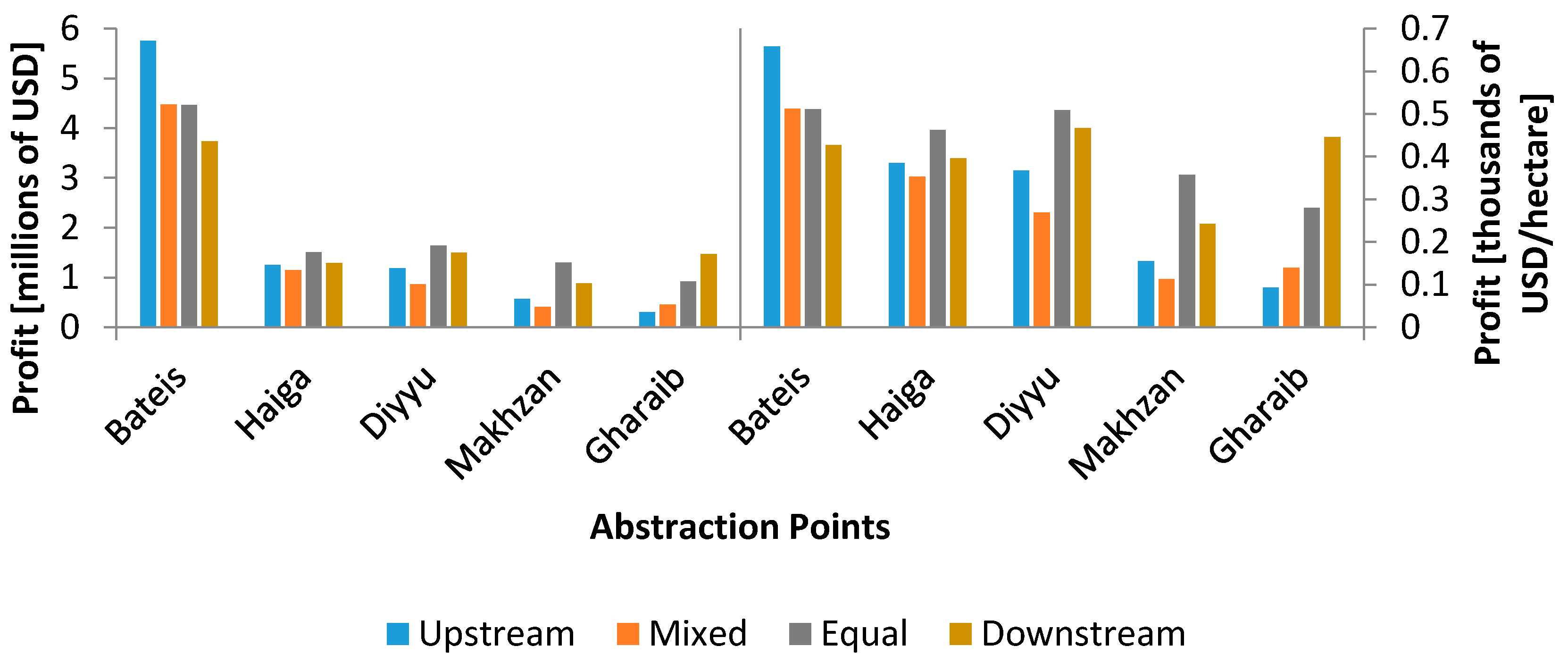
When implementing the upstream, downstream or mixed priorities, there are high levels of disparity in water demand satisfaction. Although each command area is provided supplementary volumes of groundwater throughout the year, an inequitable sharing of surface water still has significant economic and social impacts on the Abyan region. The aggregate average annual profit for all command areas is greatest with the equal priority allocation rule ($9.8 M). With upstream priority, the aggregate annual profit drops 8% to $9.1 M. The aggregate annual profit with a downstream priority is even lower at $8.9 M, nearly 10% below the equal priority’s annual profit. One reason the downstream priority performs worse than the upstream priority is the effects of transmission losses. As the water travel distance increases, so too does the amount of water lost (Appendix A). The worst performing strategy in terms of aggregate annual profit was the mixed priority ($7.4 M). The profit for each diversion weir and water allocation strategy is detailed in Figure 5.
Figure 5 shows each diversion weir’s average annual profit as well as the average profit per hectare. When evaluating a water allocation strategy such as the upstream priority we can see that the profit per hectare varies drastically amongst diversion weirs. Profit per hectare is 310% higher for Bateis than it is for Gharaib when upstream users receive priority; under equal priority, this is reduced to 190%. This suggests that the equal priority is a more equitable strategy, and as discussed earlier, a more profitable strategy for the region as a whole.
A comparison of the agricultural decisions made with the upstream and equal allocation scenarios reveals further impacts that different water allocation strategies may have. The crop mix for each allocation scenario is detailed for every command area in Figure 6.
The most striking differences occur at command areas further downstream. With the upstream priority there is very little crop variety for the eight command areas furthest from the source of water (D1 through G3). The low levels of expected inflow resulted in no more than two crops being selected for any of these command areas. The crop selection consisted of cotton, tomato or sweet melon—all of which have relatively low water requirements. Under the equal priority scenario, the number of crops selected increased for every command area with the exception of Diyyu 1 (D1) and Gharaib 3 (G3), showing higher allocations lead to more crop diversity. In addition to the increase in crop variability there was an increase in the hectares of cropping area under the equal priority, another meaningful impact of water allocation. As the cropping area increases, it is likely that the number of economic beneficiaries within that particular command area also increases leading to a wider distribution of benefits [4].
Figure 7 shows the equal priority scenario has a consistently high percentage of irrigable land used. Under the equal priority scenario an annual average of 46.4% of Abyan’s irrigable land is used. The downstream priority decreases this to 43.3%, and the upstream priority slips further to 41.5%. The best performing strategy with regard to land use was the mixed priority at 47.8%. The difference in performance for the mixed priority scenario between profits and irrigated land may be partially attributed to the periods when water was delivered. For this allocation strategy, few command areas received water for more than three consecutive months since the priority changes seasonally (off season, Seif season, off season, Kharif season, and off season). This impedes the selection of high value crops, which typically require relatively high volumes of water throughout their cycle.
5. Discussion
This application of the proposed model to Yemen’s Abyan Delta helped evaluate different water allocation rules. This project has demonstrated the substantial impacts different water allocation strategies can have on spate irrigated systems. The timing and quantity of floods allocated to command areas directly influences the crop mix selected, profit earned, and irrigable area used. In scenarios where specific users receive allocation priority, the lower priority command areas are frequently restricted in their crop selection to those crops with low water requirements. This pattern was witnessed during implementation of the upstream and downstream allocations, which ultimately resulted in high levels of profit disparity among command areas. Although the mixed priority was more equitable than the upstream or downstream allocations, the aggregate average annual profit for the mixed priority was by far the worst, at 25% less aggregate average annual profit earned than the equal priority allocation. In addition to the highest annual profit, the equal priority resulted in lower levels of profit disparity and higher area usage than both the upstream and downstream allocations. While the equal priority is the most efficient and equitable water allocation strategy, implementation of such a distribution pattern can be hard to enforce in practice because it requires an assessment of available water before volumes are allocated to each diversion point. Users closest to the source of water will see little incentive to transition from an upstream priority strategy to an equal priority, particularly when there is no functioning organization to govern and enforce such a change [4]. A further study focusing on implementation and governance is required to endorse specific allocation policy proposals.
Several limitations of the proposed model exist and could be improved upon. In our model, the water allocation and crop choice models are not dynamically linked and annual demands at each weir were fixed. In reality, demands likely respond to annual conditions and vary dynamically with cropping decisions. Limitations of the crop choice model include that the cycle length for any particular cropping decision is assumed to be the longest crop cycle length within that crop selection. Accordingly, the next planting decision is not considered until all crops have completed their cycle. Once a crop mix is selected, all crops are planted in the same time-step. Groundwater deliveries are currently fixed in the model, which could be improved to represent more strategic and realistic use of groundwater.
Limitations of the Abyan Delta proof-of-concept application should also be noted. The water conveyance model ignores illegal diversions which have significant impacts and assumes all weirs and diversion structures are always operational, which is unlikely. Economic information and some crop coefficients for these crops were difficult to attain for the Abyan region and taken from different sources, potentially leading to inconsistencies. Lack of data on crop coefficients led to various assumptions, for example scaled Kc coefficients were applied during the crop development stage. When calculating the bare soil moisture, the saturation coefficient and wilting point were considered as boundaries. Input water exceeding saturation coefficient is considered as runoff whilst amounts of water under wilting point are considered lost by deep percolation. In calculating deep percolation the soil profile was treated as a single compartment with homogeneous composition and humidity [27]. It was also assumed that the soil moisture continuously decreases at a constant rate throughout the day. A shortage of data also existed for hydrological information, with the Atkins (1984) Abyan Delta dataset recorded from 1951 to 1965 being the most up-to-date we had access to. Surface water diversions are supplied twice a month following Mehari et al. [10]. Ground water irrigation (Appendix B) is assumed to be spread evenly throughout the year and determined for each of the 18 command areas based on Salm et al. [30].
Despite these limitations and simplifications, the proof-of-concept model helped us develop our understanding of the Abyan Delta spate irrigation system and the impact of different water allocation approaches. Future improvements could include water demands that adapt to seasonal conditions and vary endogenously with cropping decisions. Improvements in soil moisture tracking, including infiltration and available soil root zone budgeting, would be beneficial. A better understanding of irrigation practices and crop choices, depths of spates, and the use and distribution of groundwater could help us more accurately model agricultural practices of the Abyan Delta. Information on observed Abyan crop choices, if available, could help us improve and calibrate the model. Because hydrological conditions have likely changed the study would need to be redone with a longer more up-to-date hydrological dataset. A possible extension of this work could be to connect the current model to an optimiser to search for economically efficient allocation regimes.
6. Conclusions
The study revealed different water diversion priority systems in Yemen’s Abyan Delta would likely result in significant differences in total water allocated, agronomical decisions and monetary impacts. The water sharing arrangements tested in our case study included upstream allocation priority, downstream priority, equal sharing of water deficits, and a mixed priority arrangement. The proof-of-concept study showed equal priority allocation is potentially the most equitable and efficient, with 8%, 10%, and 25% more net benefits than the upstream, downstream, and mixed priority scenarios, respectively. This scenario also achieved a relatively large irrigated area which means benefits are more likely to impact a wider range of beneficiaries. The idea of assigning any potential deficits amongst diverters proportionally to what they use is appealing but a separate study on the political economy of such an arrangement and its practical governance implications would need to be undertaken. The study arrived at these results using a generalised integrated assessment tool built to represent the spate irrigation management issues of the Abyan Delta. The integrated model links wadi flow allocation and soil moisture and crop yield simulators to a cropping decision model to evaluate impacts of different water allocation rules and their possible agriculture and economic implications. The crop choice simulation model is an agricultural production two-stage optimisation model of irrigation command areas where the timing, irrigated area and crop mix is decided each month based on current conditions and expected allocations. The improvement and potential use of such a model to inform water management arrangements in Yemen’s Abyan Delta and beyond would be a success if it helped reduce water conflicts.
Acknowledgments
The authors thank Henry Thompson for providing data and guidance in this UCL Environmental Systems MSc group project. Eleni Zafeiratou and Bernadett Baracskai contributed to earlier versions of Section 1 and Section 2, and Hui-Yu Chiang contributed to hydrological modelling and data processing. They are gratefully acknowledged for their valuable inputs. The authors thank Guilherme F. Marques for discussions on stochastic optimisation which influenced the formulation proposed here. The authors are responsible for all errors and omissions.
Author Contributions
Derek J. Marchant completed the water allocation modelling and drafted the paper; Alondra García Peña was responsible for the soil-moisture modelling; Derek J. Marchant and Alondra García Peña designed the crop choice model and integrated each of the models collaboratively; Mihai Tamas created the figures; and Julien Harou conceived and designed the study.
Conflicts of Interest
The authors declare no conflict of interest.
Appendix A. Transmission Loss Equation and Groundwater Values
Transmission loss within the wadi is calculated as follows.
For the equation above, V is the volume of transmission loss within one mile of travel and is the upstream volume in acre-feet. The wadi loss equation was used by Gheith and Sultan in an analysis of wadi runoff and groundwater recharge in Egypt’s Eastern Desert [31].
Appendix B. Groundwater Values
The volumes of groundwater being allotted to each command area per year are shown in Table A1.

Table A1.
Annual groundwater allotments per command area.
| Command Area | Groundwater (M/Year) |
|---|---|
| Bateis 1 | 3 |
| Bateis 2 | 7.5 |
| Bateis 3 | 7 |
| Bateis 4 | 8.5 |
| Bateis 5 | 4 |
| Bateis 6 | 3.5 |
| Haiga 1 | 2.5 |
| Haiga 2 | 2.5 |
| Haiga 3 | 2.75 |
| Haiga 4 | 1.5 |
| Diyyu 1 | 4 |
| Diyyu 2 | 2 |
| Diyyu 3 | 1.5 |
| Makhzan 1 | 2 |
| Makhzan 2 | 2 |
| Gharaib 1 | 1.75 |
| Gharaib 2 | 2 |
| Gharaib 3 | 2 |
Appendix C. Soil Moisture Tracking Model
The model estimates soil moisture by considering water losses due to bare soil evaporation, evapotranspiration of crops and deep percolation.
Appendix C.1. Bare Soil Moisture Balance
Bare soil moisture is modelled assuming it is only affected by infiltration losses. A modification to the model used in AquaCrop was made to calculate infiltration: the soil depth was considered as a single compartment [27]. Considering the corresponding characteristics (wilting point, field capacity, saturation capacity and hydraulic conductivity) outlined by Mehari, van Steenbergen and Schultz, water infiltrates the compartment at a depth where crops cannot access it [1]. Therefore, the boundaries of soil moisture are saturation capacity and wilting point, (instead of saturation and field capacity, as considered in the AquaCrop model), as can be seen in the following equations [32]:
where is the decrease in soil water content at soil depth during time step Δt (/ per day); is the drainage characteristic (dimensionless) varying from 0 (impermeable soil) to 1 (complete drainage) as a function of the hydraulic conductivity; is the actual soil water content at depth (/); is the saturation capacity (/); is the wilting point (/); and is the hydraulic conductivity at saturation (mm/day).
Water that percolates at the profile soil depth is calculated as:
where is the amount of water that percolates (mm); is the decrease in soil water content at soil depth, during time step Δt (/day); is the soil profile (m); and is the time step (day).
Appendix C.2. Crop Evapotranspiration
Water requirements for crop cycle stages are different for each crop and are affected by climatic conditions. FAO methods, as described by Allen, help determine water requirements for different crops by estimating their evapotranspiration [28]. In our soil moisture model, the water stress coefficient was taken into account. monthly values were taken from Atkins and coefficients from Allen [15,28]. Planting dates for selected crops are relevant because they affect coefficients and conditions. The final equation used to calculate crop water requirements is:
where is the evapotranspiration of the crop (mm); is the days of the cycle that correspond to the stage (days); is the crop coefficient of the stage of development (dimensionless); and is the reference crop evapotranspiration of the stage of development (mm/day).
Crop water availability is also influenced by soil characteristics. Equations from Allen (Chapters 7 and 8) were used to calculate the water stress coefficient (), the total available water in the root zone (), and immediate soil moisture availability in the root zone () [28]. represents the proportion to which the crop reduces evapotranspiration due to the lack of available water. Additionally, represents the amount of water that can be stored in the soil. is the amount of water easily available to the crop for the development stage under standard conditions. These parameters are used following Allen to estimate adjusted crop evapotranspiration [28].
Appendix C.3. Soil Moisture Balance with Crops
Soil moisture during time step t will depend on the irrigation, precipitation, evapotranspiration of the crop, runoff, capillarity rise and deep percolation. In this model, the rise in capillarity was not accounted for, as its effects are negligible when considering the high rate of groundwater depletion. The soil moisture balance was calculated as soil moisture deficit () with the following equation:
where is the root zone depletion at the end of day t and ranging from 0 to TAW (mm); is the water content in the root zone at the end of the previous day t − 1 (mm); is the precipitation on day t (mm); is the runoff from the soil surface on day t (mm); is the net irrigation depth on day t that infiltrates the soil (mm); ETc adjt is the crop evapotranspiration on day t (mm); and is the water loss out of the root zone by deep percolation on day t (mm).
FAO methodology considers precipitation to be a greater contributor than irrigation in reaching a soil’s field capacity. Precipitation is added to the monthly allocations of water and further divided into two allocations, one every 15 days (similar to Mehari, van Steenbergen and Schultz) [1]. This amount is constrained by the spate. More specifically, the physical boundary in the fields when considered at a height of 72 cm [15]. is the total requirement for three different crops. corresponds to the value calculated for the bare soil moisture during a specific time step. This deficit is transformed into available soil moisture by subtracting the deficit from field capacity. This calculation is subject to the constraint below.
Equation (A9) is based on the fact that the soil water deficit () cannot be greater than the , the wilting point. When soil moisture reaches the wilting point, the crop is unable to absorb water due to the forces that interact between the soil and the water particles. If is below 0, it represents a surplus. To calculate the initial value of , (), Equation (A10) is used.
For this calculation, the following conditions are considered: represents the average soil moisture for the effective root zone in the previous time step on the bare soil moisture calculation; precipitation is a user input.
Appendix C.4. Input Data for Agricultural and Crop Choice Models
Input data for the agriculture model consist of:
- Soil and its characteristics (type, field capacity, wilting point, saturation capacity, hydraulic conductivity at saturation, and soil depth);
- Crop water requirements (crop, crop coefficient, days of the cycle, root depth, average fraction of total available soil water that can be depleted before moisture stress, yield, and yield respond factor); and
- Physical conditions (monthly water allocation, daily , spate height, and area requirements for each crop).
Appendix D. Crop Parameters
The water requirement estimated for each of the crops is displayed in Table A2. Water requirements are shown for the entirety of each crop cycle, and further broken down to monthly requirements. These values were estimated using FAO methods described by Allen [28].
Table A2.
Annual and monthly water requirements by crop.
| Crop | Water Requirement Per Cycle (mm H2O) | Water Requirement Per Cycle (m3/ha) | Water Requirement (mm/ha) by Month | |||||||||||
|---|---|---|---|---|---|---|---|---|---|---|---|---|---|---|
| Month 1 | Month 2 | Month 3 | Month 4 | Month 5 | Month 6 | Month 7 | Month 8 | Month 9 | Month 10 | Month 11 | Month 12 | |||
| Tomato—January (135d) | 562.8 | 5628.28 | 74.3 | 80.2 | 150.6 | 182.2 | 75.5 | 0.0 | 0.0 | 0.0 | 0.0 | 0.0 | 0.0 | 0.0 |
| Tomato—January (155d) | 709.3 | 7092.88 | 73.8 | 80.2 | 165.7 | 202.9 | 162.0 | 24.7 | 0.0 | 0.0 | 0.0 | 0.0 | 0.0 | 0.0 |
| Sorghum—March | 594.8 | 5948.23 | 60.1 | 113.0 | 207.6 | 166.6 | 47.5 | 0.0 | 0.0 | 0.0 | 0.0 | 0.0 | 0.0 | 0.0 |
| Sorghum—April | 601.4 | 6013.78 | 67.5 | 121.1 | 203.6 | 160.4 | 48.8 | 0.0 | 0.0 | 0.0 | 0.0 | 0.0 | 0.0 | 0.0 |
| Tomato—April (155d) | 743.2 | 7431.65 | 105.7 | 109.4 | 142.2 | 205.3 | 157.1 | 23.5 | 0.0 | 0.0 | 0.0 | 0.0 | 0.0 | 0.0 |
| Tomato—April (145d) | 708.9 | 7088.79 | 105.7 | 108.7 | 177.7 | 194.8 | 122.0 | 0.0 | 0.0 | 0.0 | 0.0 | 0.0 | 0.0 | 0.0 |
| Cotton—April (195d) | 290.9 | 2908.91 | 61.6 | 7.1 | 9.3 | 13.4 | 45.8 | 105.7 | 48.2 | 0.0 | 0.0 | 0.0 | 0.0 | 0.0 |
| Cotton—April (180d) | 258.8 | 2587.54 | 61.6 | 7.1 | 9.3 | 13.4 | 61.8 | 105.7 | 0.0 | 0.0 | 0.0 | 0.0 | 0.0 | 0.0 |
| Sorghum—May | 566.2 | 5661.58 | 72.3 | 118.8 | 196.0 | 155.6 | 23.5 | 0.0 | 0.0 | 0.0 | 0.0 | 0.0 | 0.0 | 0.0 |
| Tomato—May (155d) | 740.9 | 7408.63 | 113.2 | 107.4 | 136.9 | 210.8 | 151.2 | 21.4 | 0.0 | 0.0 | 0.0 | 0.0 | 0.0 | 0.0 |
| Tomato—May (145d) | 708.4 | 7083.90 | 113.2 | 106.6 | 171.1 | 200.1 | 117.4 | 0.0 | 0.0 | 0.0 | 0.0 | 0.0 | 0.0 | 0.0 |
| Groundnut—Dry season (130d) | 587.7 | 5876.91 | 81.0 | 106.4 | 204.9 | 160.1 | 35.2 | 0.0 | 0.0 | 0.0 | 0.0 | 0.0 | 0.0 | 0.0 |
| Groundnut—Dry season (140d) | 577.9 | 5778.54 | 75.5 | 101.0 | 170.8 | 160.1 | 70.4 | 0.0 | 0.0 | 0.0 | 0.0 | 0.0 | 0.0 | 0.0 |
| Groundnut—May (140) | 577.2 | 5772.49 | 75.5 | 101.0 | 136.6 | 193.7 | 70.4 | 0.0 | 0.0 | 0.0 | 0.0 | 0.0 | 0.0 | 0.0 |
| Cotton—May | 278.0 | 2779.76 | 66.0 | 6.9 | 8.9 | 13.7 | 44.0 | 96.3 | 42.0 | 0.0 | 0.0 | 0.0 | 0.0 | 0.0 |
| Soy Bean—May | 677.5 | 6774.94 | 99.1 | 124.2 | 204.9 | 190.6 | 58.7 | 0.0 | 0.0 | 0.0 | 0.0 | 0.0 | 0.0 | 0.0 |
| Egg Plant—May | 644.0 | 6439.65 | 113.2 | 97.2 | 140.3 | 187.6 | 105.7 | 0.0 | 0.0 | 0.0 | 0.0 | 0.0 | 0.0 | 0.0 |
| Millet—June | 389.3 | 3892.55 | 74.0 | 148.5 | 140.3 | 26.4 | 0.0 | 0.0 | 0.0 | 0.0 | 0.0 | 0.0 | 0.0 | 0.0 |
| Sorghum—June | 557.7 | 5576.85 | 71.0 | 114.3 | 201.3 | 149.7 | 21.4 | 0.0 | 0.0 | 0.0 | 0.0 | 0.0 | 0.0 | 0.0 |
| Groundnut—June | 562.2 | 5621.80 | 74.0 | 97.3 | 140.3 | 186.4 | 64.2 | 0.0 | 0.0 | 0.0 | 0.0 | 0.0 | 0.0 | 0.0 |
| Sesame—June | 438.5 | 4384.55 | 77.1 | 130.7 | 201.3 | 29.4 | 0.0 | 0.0 | 0.0 | 0.0 | 0.0 | 0.0 | 0.0 | 0.0 |
| Soy Bean—June | 744.1 | 7440.90 | 97.2 | 153.7 | 210.5 | 202.5 | 80.3 | 0.0 | 0.0 | 0.0 | 0.0 | 0.0 | 0.0 | 0.0 |
| Egg Plant—June | 625.5 | 6255.30 | 111.1 | 93.6 | 144.1 | 180.5 | 96.3 | 0.0 | 0.0 | 0.0 | 0.0 | 0.0 | 0.0 | 0.0 |
| Sweet Melon—August | 490.3 | 4903.41 | 70.9 | 97.6 | 152.5 | 133.1 | 36.3 | 0.0 | 0.0 | 0.0 | 0.0 | 0.0 | 0.0 | 0.0 |
| Cotton—September | 245.3 | 2452.91 | 61.6 | 6.0 | 7.0 | 9.1 | 31.0 | 83.5 | 47.1 | 0.0 | 0.0 | 0.0 | 0.0 | 0.0 |
| Maize (grain)—October | 392.2 | 3921.94 | 64.2 | 98.1 | 145.1 | 73.8 | 11.0 | 0.0 | 0.0 | 0.0 | 0.0 | 0.0 | 0.0 | 0.0 |
| Maize (sweet)—October | 305.3 | 3053.26 | 62.9 | 107.4 | 135.1 | 0.0 | 0.0 | 0.0 | 0.0 | 0.0 | 0.0 | 0.0 | 0.0 | 0.0 |
| Tomato—October | 699.0 | 6990.20 | 96.3 | 81.3 | 92.9 | 142.7 | 160.4 | 125.5 | 0.0 | 0.0 | 0.0 | 0.0 | 0.0 | 0.0 |
| Tomato—November | 731.3 | 7313.24 | 84.1 | 70.1 | 95.2 | 160.4 | 180.7 | 140.9 | 0.0 | 0.0 | 0.0 | 0.0 | 0.0 | 0.0 |
| Soy Bean—December | 295.6 | 2956.29 | 65.0 | 142.5 | 88.2 | 0.0 | 0.0 | 0.0 | 0.0 | 0.0 | 0.0 | 0.0 | 0.0 | 0.0 |
| Sweet Melon—December | 527.8 | 5278.48 | 36.3 | 58.9 | 99.2 | 149.1 | 146.8 | 37.7 | 0.0 | 0.0 | 0.0 | 0.0 | 0.0 | 0.0 |
| Maize (grain)—December (140d) | 475.9 | 4759.03 | 42.3 | 74.3 | 153.1 | 150.4 | 55.8 | 0.0 | 0.0 | 0.0 | 0.0 | 0.0 | 0.0 | 0.0 |
| Maize (sweet)—December (90d) | 297.8 | 2978.38 | 47.4 | 95.0 | 155.5 | 0.0 | 0.0 | 0.0 | 0.0 | 0.0 | 0.0 | 0.0 | 0.0 | 0.0 |
Daily evapotranspiration segmented by month is displayed in Table A3 for each crop. These values were estimated as described in Appendix C.
Table A3.
Crop daily evapotranspiration by month.
| Crop | Eto Daily (mm) by Month | |||||||||||
|---|---|---|---|---|---|---|---|---|---|---|---|---|
| Month 1 | Month 2 | Month 3 | Month 4 | Month 5 | Month 6 | Month 7 | Month 8 | Month 9 | Month 10 | Month 11 | Month 12 | |
| Tomato—January (135d) | 4.13 | 4.64 | 5.23 | 5.87 | 6.29 | 6.17 | 5.94 | 6.10 | 5.87 | 5.35 | 4.67 | 4.03 |
| Tomato—January (155d) | 4.13 | 4.64 | 5.23 | 5.87 | 6.29 | 6.17 | 5.94 | 6.10 | 5.87 | 5.35 | 4.67 | 4.03 |
| Sorghum—March | 5.23 | 5.87 | 6.29 | 6.17 | 5.94 | 6.10 | 5.87 | 5.35 | 4.67 | 4.03 | 4.13 | 4.64 |
| Sorghum—April | 5.87 | 6.29 | 6.17 | 5.94 | 6.10 | 5.87 | 5.35 | 4.67 | 4.03 | 4.13 | 4.64 | 5.23 |
| Tomato—April (155d) | 5.87 | 6.29 | 6.17 | 5.94 | 6.10 | 5.87 | 5.35 | 4.67 | 4.03 | 4.13 | 4.64 | 5.23 |
| Tomato—April (145d) | 5.87 | 6.29 | 6.17 | 5.94 | 6.10 | 5.87 | 5.35 | 4.67 | 4.03 | 4.13 | 4.64 | 5.23 |
| Cotton—April (195d) | 5.87 | 6.29 | 6.17 | 5.94 | 6.10 | 5.87 | 5.35 | 4.67 | 4.03 | 4.13 | 4.64 | 5.23 |
| Cotton—April (180d) | 5.87 | 6.29 | 6.17 | 5.94 | 6.10 | 5.87 | 5.35 | 4.67 | 4.03 | 4.13 | 4.64 | 5.23 |
| Sorghum—May | 6.29 | 6.17 | 5.94 | 6.10 | 5.87 | 5.35 | 4.67 | 4.03 | 4.13 | 4.64 | 5.23 | 5.87 |
| Tomato—May (155d) | 6.29 | 6.17 | 5.94 | 6.10 | 5.87 | 5.35 | 4.67 | 4.03 | 4.13 | 4.64 | 5.23 | 5.87 |
| Tomato—May (145d) | 6.29 | 6.17 | 5.94 | 6.10 | 5.87 | 5.35 | 4.67 | 4.03 | 4.13 | 4.64 | 5.23 | 5.87 |
| Groundnut—Dry season (130d) | 6.29 | 6.17 | 5.94 | 6.10 | 5.87 | 5.35 | 4.67 | 4.03 | 4.13 | 4.64 | 5.23 | 5.87 |
| Groundnut—Dry season (140d) | 6.29 | 6.17 | 5.94 | 6.10 | 5.87 | 5.35 | 4.67 | 4.03 | 4.13 | 4.64 | 5.23 | 5.87 |
| Groundnut—May (140) | 6.29 | 6.17 | 5.94 | 6.10 | 5.87 | 5.35 | 4.67 | 4.03 | 4.13 | 4.64 | 5.23 | 5.87 |
| Cotton—May | 6.29 | 6.17 | 5.94 | 6.10 | 5.87 | 5.35 | 4.67 | 4.03 | 4.13 | 4.64 | 5.23 | 5.87 |
| Soy Bean—May | 6.29 | 6.17 | 5.94 | 6.10 | 5.87 | 5.35 | 4.67 | 4.03 | 4.13 | 4.64 | 5.23 | 5.87 |
| Egg Plant—May | 6.29 | 6.17 | 5.94 | 6.10 | 5.87 | 5.35 | 4.67 | 4.03 | 4.13 | 4.64 | 5.23 | 5.87 |
| Millet—June | 6.17 | 5.94 | 6.10 | 5.87 | 5.35 | 4.67 | 4.03 | 4.13 | 4.64 | 5.23 | 5.87 | 6.29 |
| Sorghum—June | 6.17 | 5.94 | 6.10 | 5.87 | 5.35 | 4.67 | 4.03 | 4.13 | 4.64 | 5.23 | 5.87 | 6.29 |
| Groundnut—June | 6.17 | 5.94 | 6.10 | 5.87 | 5.35 | 4.67 | 4.03 | 4.13 | 4.64 | 5.23 | 5.87 | 6.29 |
| Sesame—June | 6.17 | 5.94 | 6.10 | 5.87 | 5.35 | 4.67 | 4.03 | 4.13 | 4.64 | 5.23 | 5.87 | 6.29 |
| Soy Bean—June | 6.17 | 5.94 | 6.10 | 5.87 | 5.35 | 4.67 | 4.03 | 4.13 | 4.64 | 5.23 | 5.87 | 6.29 |
| Egg Plant—June | 6.17 | 5.94 | 6.10 | 5.87 | 5.35 | 4.67 | 4.03 | 4.13 | 4.64 | 5.23 | 5.87 | 6.29 |
| Sweet Melon—August | 6.10 | 5.87 | 5.35 | 4.67 | 4.03 | 4.13 | 4.64 | 5.23 | 5.87 | 6.29 | 6.17 | 5.94 |
| Cotton—September | 5.87 | 5.35 | 4.67 | 4.03 | 4.13 | 4.64 | 5.23 | 5.87 | 6.29 | 6.17 | 5.94 | 6.10 |
| Maize (grain)—October | 5.35 | 4.67 | 4.03 | 4.13 | 4.64 | 5.23 | 5.87 | 6.29 | 6.17 | 5.94 | 6.10 | 5.87 |
| Maize (sweet)—October | 5.35 | 4.67 | 4.03 | 4.13 | 4.64 | 5.23 | 5.87 | 6.29 | 6.17 | 5.94 | 6.10 | 5.87 |
| Tomato—October | 5.35 | 4.67 | 4.03 | 4.13 | 4.64 | 5.23 | 5.87 | 6.29 | 6.17 | 5.94 | 6.10 | 5.87 |
| Tomato—November | 4.67 | 4.03 | 4.13 | 4.64 | 5.23 | 5.87 | 6.29 | 6.17 | 5.94 | 6.10 | 5.87 | 5.35 |
| Soy Bean—December | 4.03 | 4.13 | 4.64 | 5.23 | 5.87 | 6.29 | 6.17 | 5.94 | 6.10 | 5.87 | 5.35 | 4.67 |
| Sweet Melon—December | 4.03 | 4.13 | 4.64 | 5.23 | 5.87 | 6.29 | 6.17 | 5.94 | 6.10 | 5.87 | 5.35 | 4.67 |
| Maize (grain)—December (140d) | 4.03 | 4.13 | 4.64 | 5.23 | 5.87 | 6.29 | 6.17 | 5.94 | 6.10 | 5.87 | 5.35 | 4.67 |
| Maize (sweet)—December (90d) | 4.03 | 4.13 | 4.64 | 5.23 | 5.87 | 6.29 | 6.17 | 5.94 | 6.10 | 5.87 | 5.35 | 4.67 |
Specifics on the length of each crop cycle, the plant month and considerations for determining the expected profit are presented in Table A4 [15,16,19].
Table A4.
Crop parameters for determining expected profit.
| Crop | Days in Cycle | Plant Date | Yield (kg/ha) | Expected Revenue (YR/kg) | Market Price (YR/ha) | Cost of Production (YR/ha) |
|---|---|---|---|---|---|---|
| Tomato—January (135d) | 135 | January | 20,283 | 25 | 676,100 | 166,711 |
| Tomato—January (155d) | 155 | January | 20,283 | 25 | 676,100 | 166,711 |
| Sorghum—March | 130 | March | 1762 | 41 | 137,520 | 64,505 |
| Sorghum—April | 130 | April | 1762 | 41 | 137,520 | 64,505 |
| Tomato—April (155d) | 155 | April | 20,283 | 25 | 676,100 | 166,711 |
| Tomato—April (145d) | 145 | April | 20,283 | 25 | 676,100 | 166,711 |
| Cotton—April (195d) | 195 | April | 1366 | 23 | 153,684 | 121,690 |
| Cotton—April (180d) | 180 | April | 1366 | 23 | 153,684 | 121,690 |
| Sorghum—May | 125 | May | 1762 | 41 | 137,520 | 64,505 |
| Tomato—May (155d) | 155 | May | 20,283 | 25 | 676,100 | 166,711 |
| Tomato—May (145d) | 145 | May | 20,283 | 25 | 676,100 | 166,711 |
| Groundnut—Dry season (130d) | 130 | May | 1897 | 128 | 379,400 | 137,000 |
| Groundnut—Dry season (140d) | 140 | May | 1897 | 128 | 379,400 | 137,000 |
| Groundnut—May (140) | 140 | May | 1897 | 128 | 379,400 | 137,000 |
| Cotton—May | 195 | May | 1366 | 23 | 153,684 | 121,690 |
| Soy Bean—May | 140 | May | 2000 | 1 | 2688 | 65,000 |
| Egg Plant—May | 140 | May | 60,000 | 3 | 167,568 | 80,000 |
| Millet—June | 105 | June | 500 | 64 | 153,684 | 121,690 |
| Sorghum—June | 125 | June | 1,762 | 41 | 137,520 | 64,505 |
| Groundnut—June | 140 | June | 1,897 | 128 | 379,400 | 137,000 |
| Sesame—June | 110 | June | 536 | 280 | 219,273 | 69,200 |
| Soy Bean—June | 150 | June | 2000 | 1 | 2688 | 65,000 |
| Egg Plant—June | 140 | June | 60,000 | 3 | 167,568 | 80,000 |
| Sweet Melon—August | 135 | August | 15,476 | 19 | 429,157 | 141,000 |
| Cotton—September | 195 | September | 1366 | 23 | 153,684 | 121,690 |
| Maize (grain)—October | 125 | October | 1200 | 61 | 137,520 | 64,505 |
| Maize (sweet)—October | 90 | October | 1200 | 61 | 137,520 | 64,505 |
| Tomato—October | 180 | October | 20,283 | 25 | 676,100 | 166,711 |
| Tomato—November | 180 | November | 20,283 | 25 | 676,100 | 166,711 |
| Soy Bean—December | 85 | December | 2000 | 1 | 2688 | 65,000 |
| Sweet Melon—December | 160 | December | 15,476 | 19 | 429,157 | 141,000 |
| Maize (grain)—December (140d) | 140 | December | 1200 | 61 | 137,520 | 64,505 |
| Maize (sweet)—December (90d) | 90 | December | 1200 | 61 | 137,520 | 64,505 |
References
- Mehari, A.; Steenbergen, F.; Schultz, B. Water Rights and Rules, and Management in Spate Irrigation Systems in Eritrea, Yemen and Pakistan; International Water Management Institute (IWMI): Colombo, Sri Lanka, 2007. [Google Scholar]
- Almas, A.; Scholz, M. Agriculture and water resources crisis in Yemen: Need for sustainable agriculture. J. Sustain. Agric. 2006, 28, 55–75. [Google Scholar] [CrossRef]
- Noaman, A.; Haidera, M.; Othman, S.; Kebsi, K.; Babaqi, A. Adapting to Water Scarcity for Yemen’s Vulnerable Communities, Case Study: Aden City; The Netherlands Climate Assistance Programme: Leusden, The Netherlands, 2007. [Google Scholar]
- Thompson, H.; (University College London, London, United Kingdom). Personal Communication, 2012.
- Muggah, R.; Hales, G.; LeBrun, E.; Potter, A.; Jones, R. Under Pressure: Social Violence over Land and Water in Yemen; Yemen Armed Violence Assessment: Geneva, Switzerland, 2010. [Google Scholar]
- The International Fund for Agricultural Development (IFAD). Republic of Yemen Economic Opportunities Programme; The International Fund for Agricultural Development: Rome, Italy, 2010. [Google Scholar]
- Haidera, M.; Noaman, A.; Alhakimi, S.; Kebsi, A.A.; Noaman, A.; Fencl, A.; Dougherty, B.; Swartz, C. Water scarcity and climate change adaptation for Yemen’s vulnerable communities, Local Environment. Int. J. Justice Sustain. 2011, 16, 473–488. [Google Scholar]
- Ghebremariam, B.H.; van Steenbergen, F. Agricultural Water Management in Ephemeral Rivers: Community Management in Spate Irrigation in Eritrea. Afr. Water J. 2007, 1, 48–65. [Google Scholar]
- El-Askari, K. Investigating the Potential for Efficient Water Management in Spate Irrigation Schemes Using the Spate Management model. J. Appl. Irrig. Sci. 2005, 40, 177–192. [Google Scholar]
- Mehari, A.; Schultz, B.; Depeweg, H.; Laat, P.D. Modelling Soil moisture and assessing its impacts on water sharing and crop yield for the Wadi Laba spate irrigation system, Eritrea. Irrig. Drain. 2008, 57, 42–56. [Google Scholar] [CrossRef]
- Ward, F.A.; Amer, S.A.; Ziaee, F. Water allocation rules in Afghanistan for improved food security. Food Secur. 2013, 5, 35–53. [Google Scholar] [CrossRef]
- Thompson, H. LadyBird Book Abyan. Unpublished work. 2012. [Google Scholar]
- Pelgrum, H.; Bastiaanssen, W.; Voogt, M.; Berghege, M. Satellite Imagery for Cropping Pattern and Irrigated Area Monitoring Final Report; WaterWatch: Sana’a, Yemen, 2009; p. 90. [Google Scholar]
- Voogt, M.; Soppe, R.; Noordman, E. Satellite Imagery for Cropping Pattern and Irrigated Area Monitoring Interim Report; WaterWatch: Sana’a, Yemen, 2007; p. 27. [Google Scholar]
- Atkins. Feasibility Study for Wadi Bana and Abyan Delta. Development Project. In Annexe A. Hydrology and Water Resources; Ministry of Agriculture and Agrarian Reform PDR of Yemen; WS Atkins & Partners, Binnie & Partners: London, UK, 1984. [Google Scholar]
- United States Agency for International Development. Yemen Irrigated Benchmark, Middle East Water and Livelihoods Initiative; United States Agency for International Development and International Center for Agricultural Research in Dry Areas: Beirut, Lebanon, 2011.
- Van Steenbergen, F.; Lawrence, P.; Haile, A.M.; Salman, M.; Faurès, J.-M. Guidelines on Spate Irrigation, Irrigation and Drainage Paper; Food and Agriculture Organization of the United Nations (FAO): Rome, Italy, 2010. [Google Scholar]
- MacDonald, A. Aspects of spate irrigation in PDR Yemen, Spate irrigation. In Proceedings of the Subregional Expert Consultation on Wadi Development for Agriculture in the Natural Yemen, Aden, PDR Yemen, 6–10 December 1987; pp. 80–90. [Google Scholar]
- Girgirah, A.A.; Maktari, M.S.; Sattar, H.A.; Mohammed, M.F.; Abbas, H.H.; Shoubihi, H.M. Wadi Development for Agriculture in PDR Yemen. In Proceedings of the Subregional Expert Consultation on Wadi Development for Agriculture in the Natural Yemen, Aden, PDR Yemen, 6–10 December 1987. [Google Scholar]
- Pelgrum, H.; Bastiaansseen, W.; Voogt, M.; Berghege, M. Satellite Imagery for Cropping and Irrigated Area Monitoring; Ministry of Agriculture and Irrigation of Republic of Yemen and World Bank: Sana’a, Yemen, 2009. [Google Scholar]
- United States Agency for International Development. Middle East Water and Livelihoods Initiative, Yemen; United States Agency for International Development and International Center for Agricultural Research in Dry Areas: Beirut, Lebanon, 2011.
- Varisco, D.M. Dancing on the Heads of Snakes in Yemen; Springer Science + Business Media: Berlin, Germany, 2011. [Google Scholar]
- Colonial Office. Report on the Abyan Scheme; Colonial Office: London, UK, 1951. [Google Scholar]
- Ba’amir, M. Agricultural Development in the People’s Democratic Republic of Yemen: Organization and Administration of the Abyan Delta Project. Graduate Thesis, Development Administration, American University of Beirut, Beirut, Lebanon, 1973. [Google Scholar]
- Ekasingh, B.; Letcher, R.A. Successes and failures to embed socioeconomic dimensions in integrated natural resource management modeling: Lessons from Thailand. Math. Comput. Simul. 2008, 78, 137–145. [Google Scholar] [CrossRef]
- Draper, A.J.; Munevar, A.; Arora, S.K.; Reyes, E.; Parker, N.L.; Chung, F.I.; Peterson, L.E. CalSim: Generalized Model for Reservoir System Analysis. J. Water Resour. Plan. Manag. 2004, 130, 480–489. [Google Scholar] [CrossRef]
- Raes, D.; Steduto, P.; Hsiao, T.; Fereres, E. Calculation procedures. AquaCrop, in Land and Water Division Reference Manual; Food and Agriculture Organization: Rome, Italy, 2012; pp. 34–39. [Google Scholar]
- Allen, R.G. Crop Evapotranspiration—Guidelines for Computing Crop Water Requirements. In FAO Irrigation and Drainage Paper 56; FAO, Ed.; FAO: Rome, Italy, 1998. [Google Scholar]
- Wardlaw, R. Computer optimisation for better water allocation. Agric. Water Manag. 1999, 40, 65–70. [Google Scholar] [CrossRef]
- Salm, S.; Bastiaanssen, W.; Voogt, M.; Kassies, R.; Al-Shaybani, H.P.; Al-Hemiary, A.-M. Satellite Imagery for Follow-Up Study Final Report; WaterWatch: Wageningen, Netherlands, 2012; p. 97. [Google Scholar]
- Gheith, H.; Sultan, M. Construction of a Hydrological Model for Estimating Wadi Runoff and Groundwater Recharge in the Easter Desert, Egypt. J. Hydrol. 2002, 263, 36–55. [Google Scholar] [CrossRef]
- United States Department of Agriculture. Irrigation, National Engineering Book; United States Department of Agriculture: Washington, DC, USA, 1991.
Figure 1.
Major irrigation weirs (5), irrigated command areas (18), and population centres of Yemen’s Abyan Delta.
Figure 1.
Major irrigation weirs (5), irrigated command areas (18), and population centres of Yemen’s Abyan Delta.
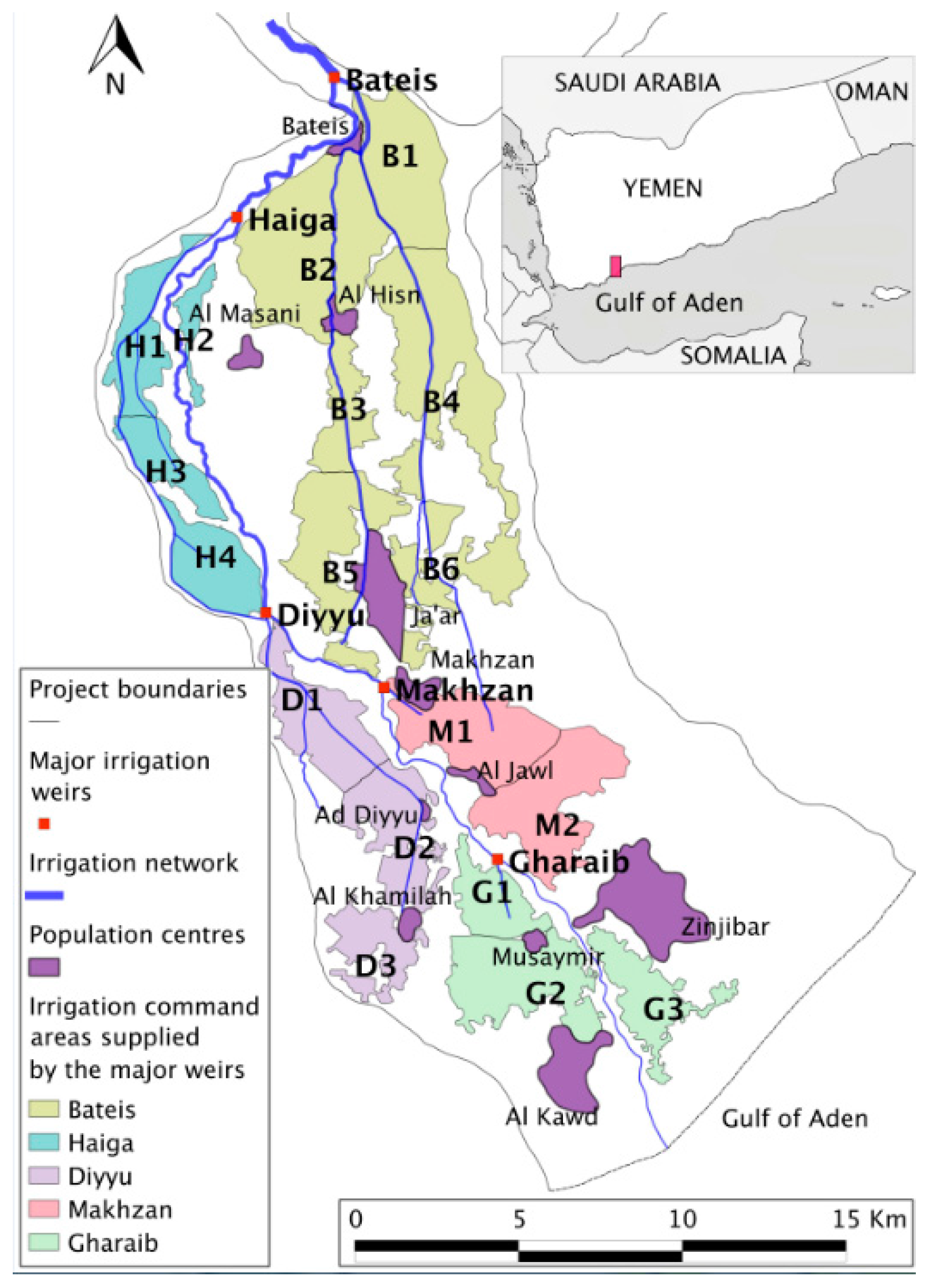
Figure 2.
Integrated model applied to all “i” irrigation command areas. Stage 1 prepares the model inputs for each command area; stage 2 simulates agronomical decisions and processes over time for each command area. The integrated simulation is run over a multi-year planning horizon (e.g., historical inflows) and a n-month “scan” period (Section 4) over which the famer makes seasonal cropping decisions.

Figure 3.
Average inflow values based on a 15-year historical period [15].
Figure 3.
Average inflow values based on a 15-year historical period [15].
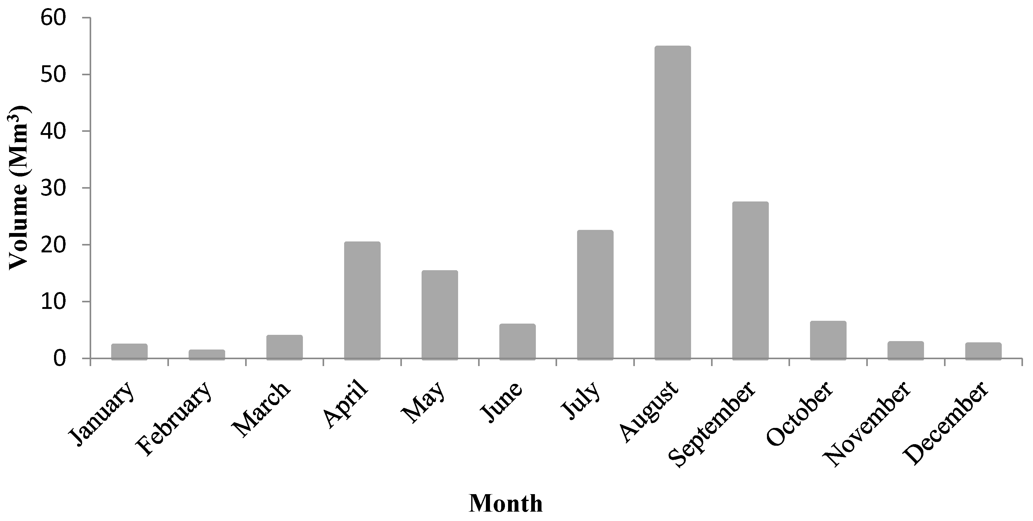
Figure 4.
Average annual water allocation in million cubic metres for the four allocation scenarios: (a) upstream; (b) downstream; (c) mixed; and (d) equal priorities.
Figure 4.
Average annual water allocation in million cubic metres for the four allocation scenarios: (a) upstream; (b) downstream; (c) mixed; and (d) equal priorities.
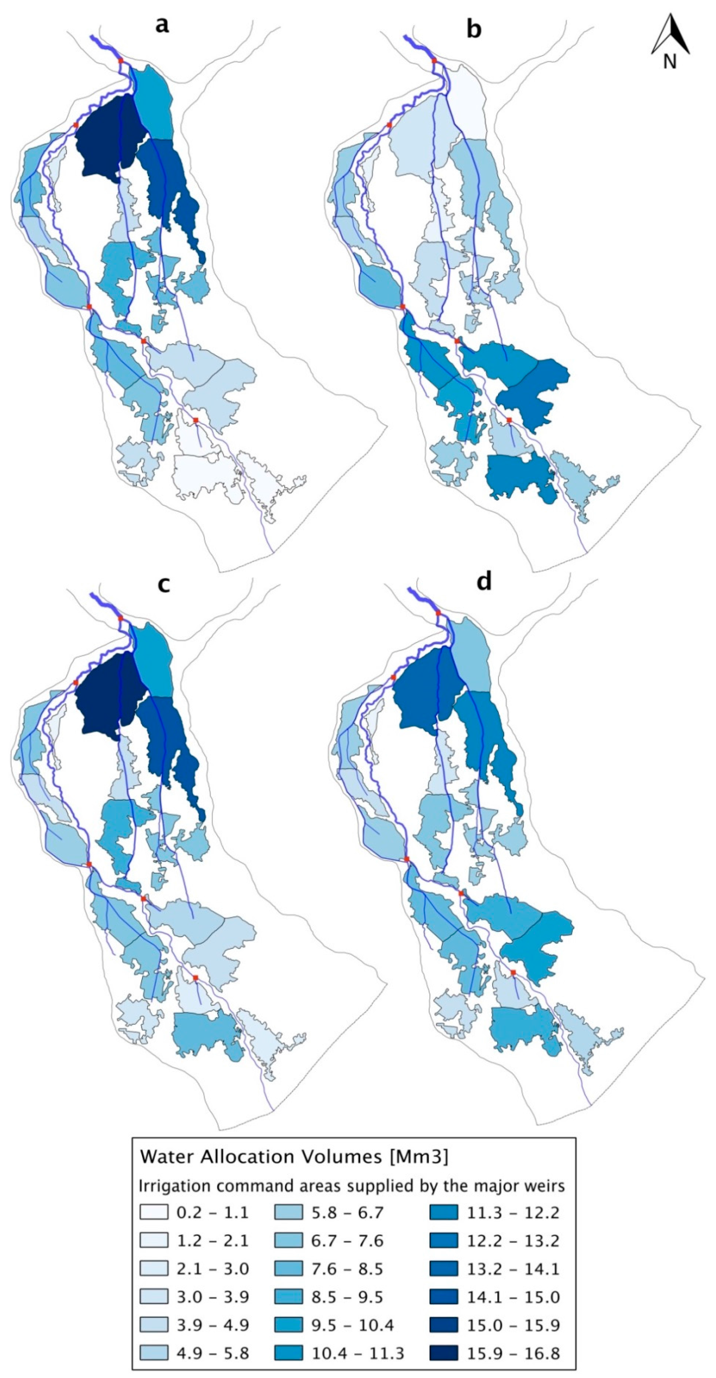
Figure 5.
Expected annual profit for areas served by each weir per water allocation scenario.

Figure 6.
Comparison of crop diversity and cropping area for each command area using the upstream and equal allocation scenarios.
Figure 6.
Comparison of crop diversity and cropping area for each command area using the upstream and equal allocation scenarios.
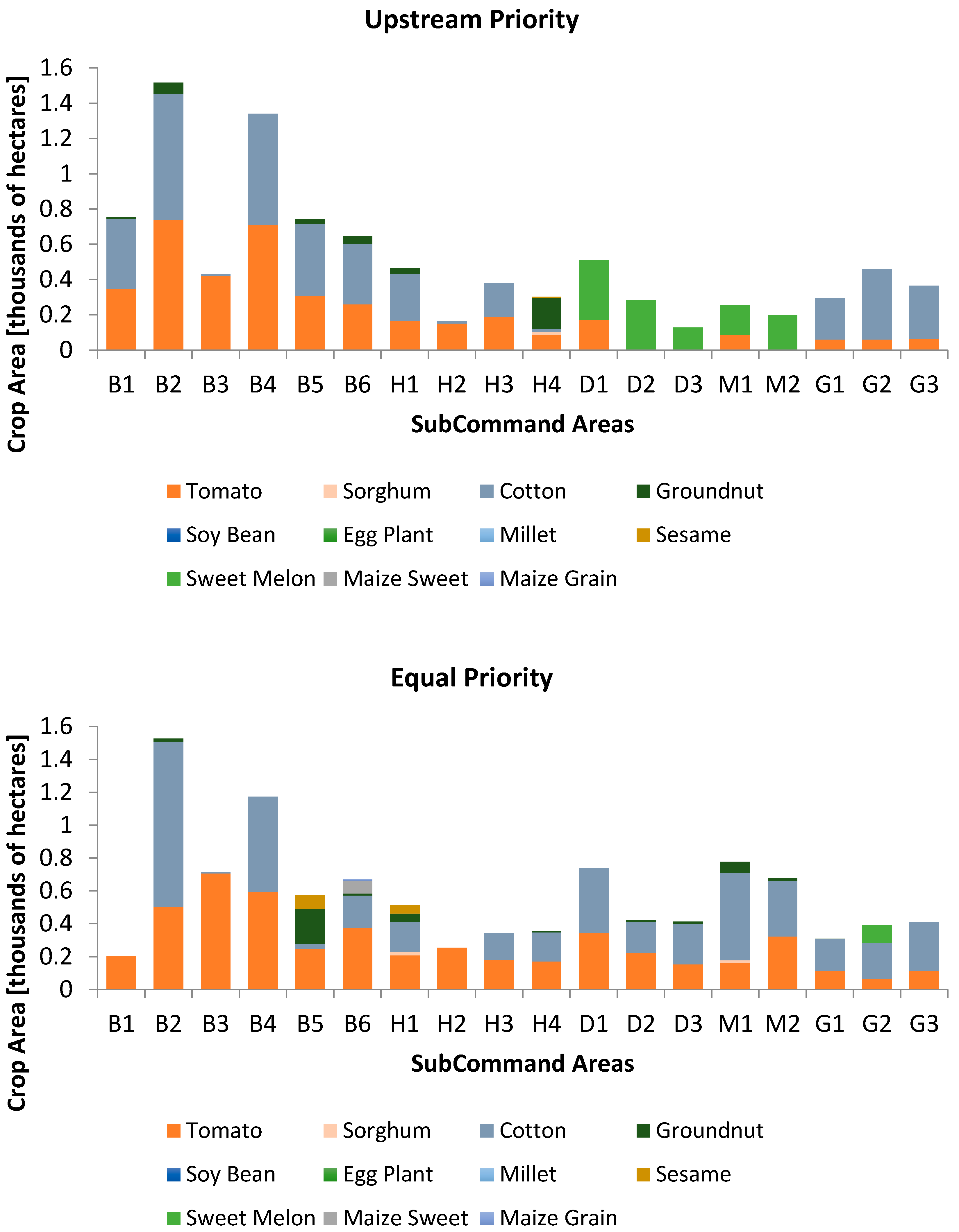
Figure 7.
Cropping area used under the different water allocation scenarios.
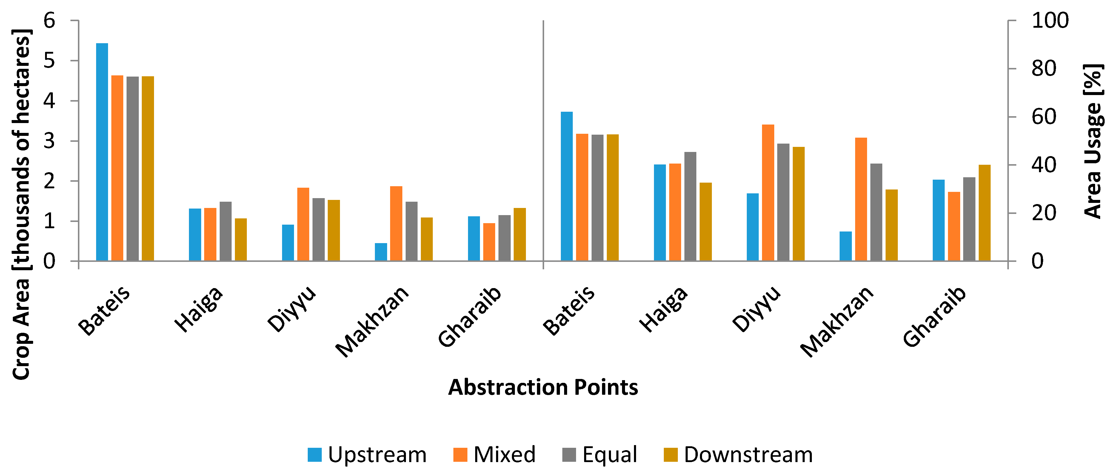
Table 1.
Input data for soil moisture model.
| Soil Characteristics | Crop Water Requirements | Physical Conditions | Actual Yields |
|---|---|---|---|
| Hydraulic conductivity at saturation Type Field capacity Wilting point Saturation capacity Soil depth | Average fraction of total available soil water that can deplete before moisture stress Crop coefficient Length of the cycle Root depth Yield Yield response factor | Daily crop evapotranspiration Spate height Water inflow | Calculated yields for specific hydrological event and location Expected profit for each crop |
Table 2.
Average percentage of water demand satisfied over the 15-year simulation.
| Allocation Priority | Water Demand Satisfied per Weir | ||||
|---|---|---|---|---|---|
| Bateis | Haiga | Diyyu | Makhzan | Gharaib | |
| Upstream | 100% | 74% | 50% | 35% | 8% |
| Mixed | 99% | 84% | 69% | 41% | 63% |
| Equal | 79% | 79% | 79% | 79% | 79% |
| Downstream | 34% | 89% | 100% | 100% | 100% |
© 2018 by the authors. Licensee MDPI, Basel, Switzerland. This article is an open access article distributed under the terms and conditions of the Creative Commons Attribution (CC BY) license (http://creativecommons.org/licenses/by/4.0/).
Share and Cite
MDPI and ACS Style
Marchant, D.J.-U.; García Peña, A.; Tamas, M.; Harou, J.J. Simulating Water Allocation and Cropping Decisions in Yemen’s Abyan Delta Spate Irrigation System. Water 2018, 10, 121. https://doi.org/10.3390/w10020121
AMA Style
Marchant DJ-U, García Peña A, Tamas M, Harou JJ. Simulating Water Allocation and Cropping Decisions in Yemen’s Abyan Delta Spate Irrigation System. Water. 2018; 10(2):121. https://doi.org/10.3390/w10020121
Chicago/Turabian StyleMarchant, Derek Jin-Uk, Alondra García Peña, Mihai Tamas, and Julien J. Harou. 2018. "Simulating Water Allocation and Cropping Decisions in Yemen’s Abyan Delta Spate Irrigation System" Water 10, no. 2: 121. https://doi.org/10.3390/w10020121
Note that from the first issue of 2016, this journal uses article numbers instead of page numbers. See further details here.