Consumption of Free Chlorine in an Aqueduct Scheme with Low Protection: Case Study of the New Aqueduct Simbrivio-Castelli (NASC), Italy

 ,
, 
 ,
,  , and
, and 
Abstract
:1. Introduction
2. Issues Related to the Use of Chlorine in Water Supply Networks
- (a)
- the consumption of residual disinfectant in the network;
- (b)
- the formation of toxic substances from the reaction of the oxidants used in the disinfection;
- (c)
- the establishment of microbial growth processes in the network.
2.1. Consumption of Free Chlorine in the Network
2.2. Final Products of Chlorine Reactions
2.3. Microbial Growth
3. Data Analysis Section—Modeling of the Chlorine Consumption with Semi-Empirical Methods
4. Materials and Methods
4.1. Characterization of the Distribution Network for Water Supply
- the water from the different sources is mixed in a longitudinal tank, called a “hydraulic gallery”; in this basin, which is the source of supply pipelines, sodium hypochlorite is added as a disinfection agent;
- the main duct branches into numerous secondary pipelines.
- flows from the different sources;
- days of interruption of the supply service;
- repair of hydraulic losses occurred on pipes;
- interruptions in the disinfection procedure.
4.2. Collection of Data on Water Quality
- (a)
- aqueduct water supply (springs and wells);
- (b)
- water procured to the aqueduct network;
- (c)
- disinfected water supplied to the supply network;
- (d)
- water transported by the supply network to the consumers.
4.3. Method of Processing Data
5. Results
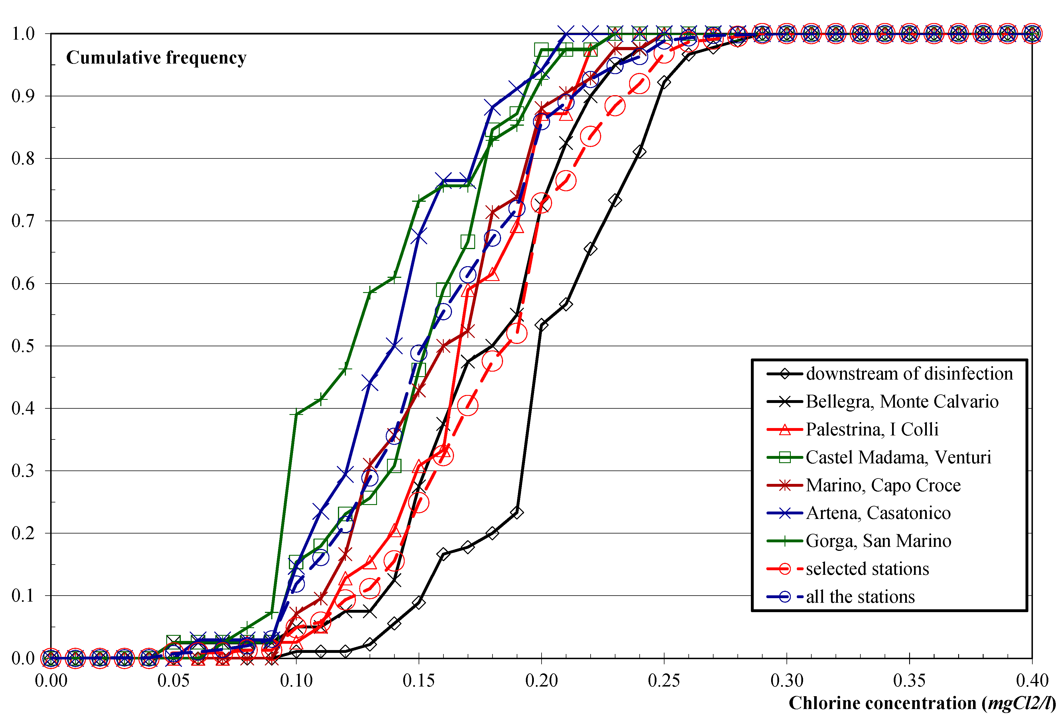
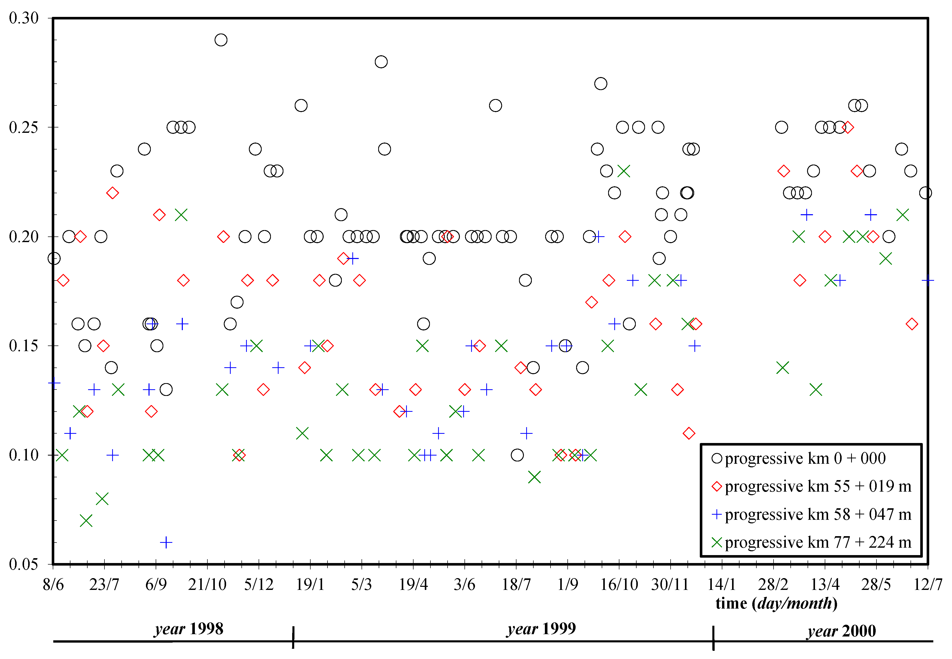
5.1. Processing of Free Chlorine Data
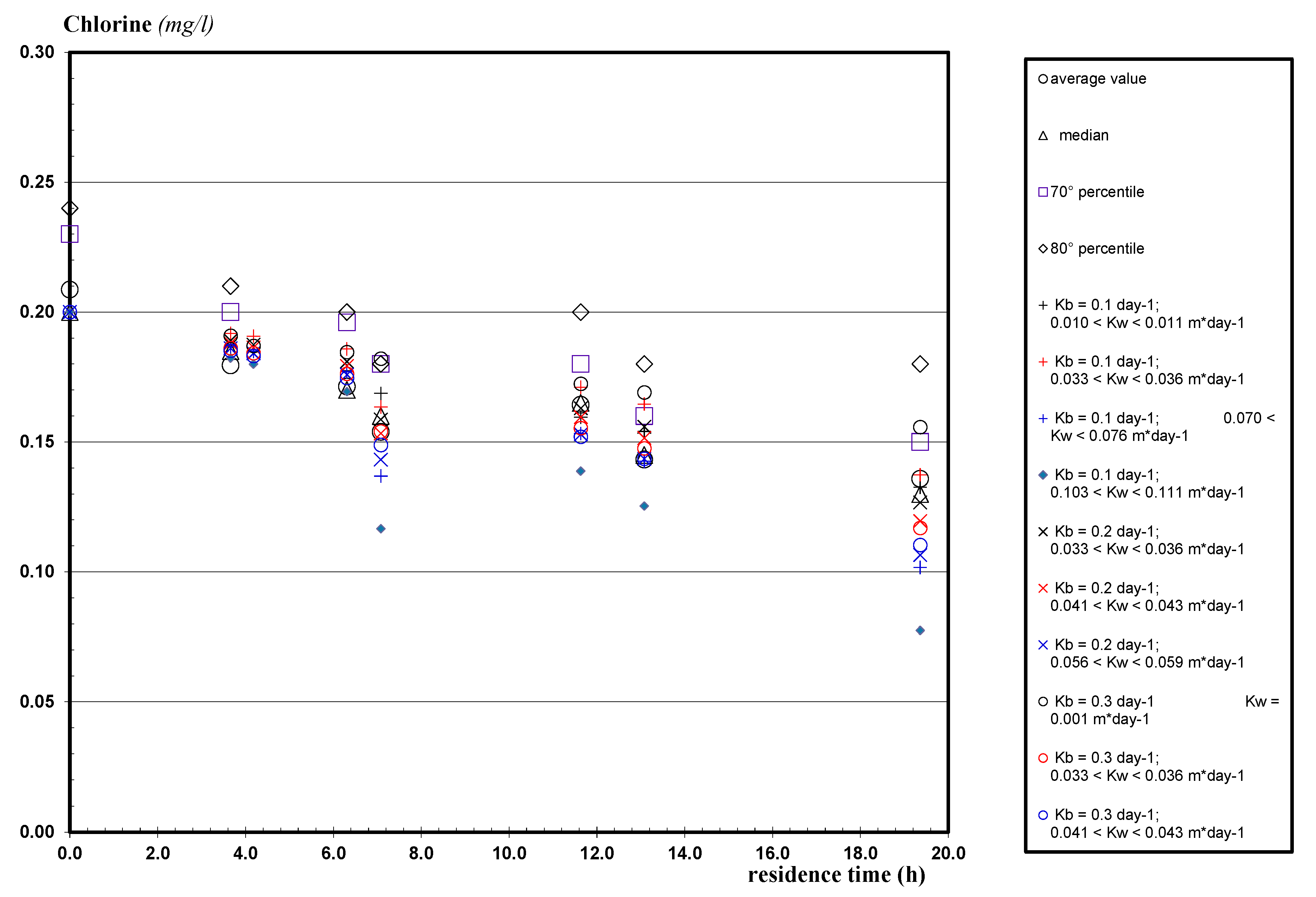
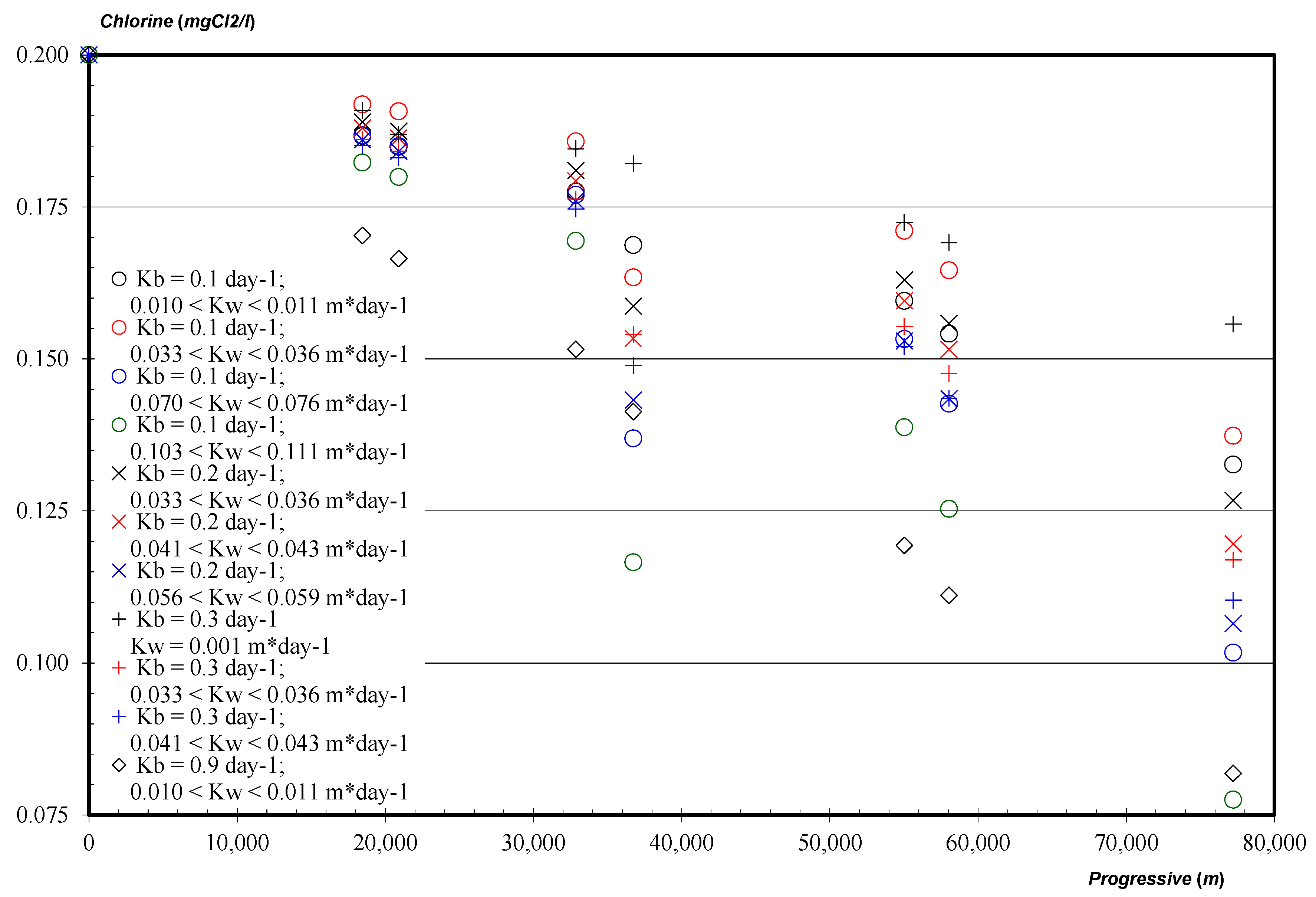
5.2. Simulations with EPANET Model
5.3. Discussion
6. Concluding Remarks
- In more than 70% of the observed data the concentration values were below 0.2 mgCl2/L.
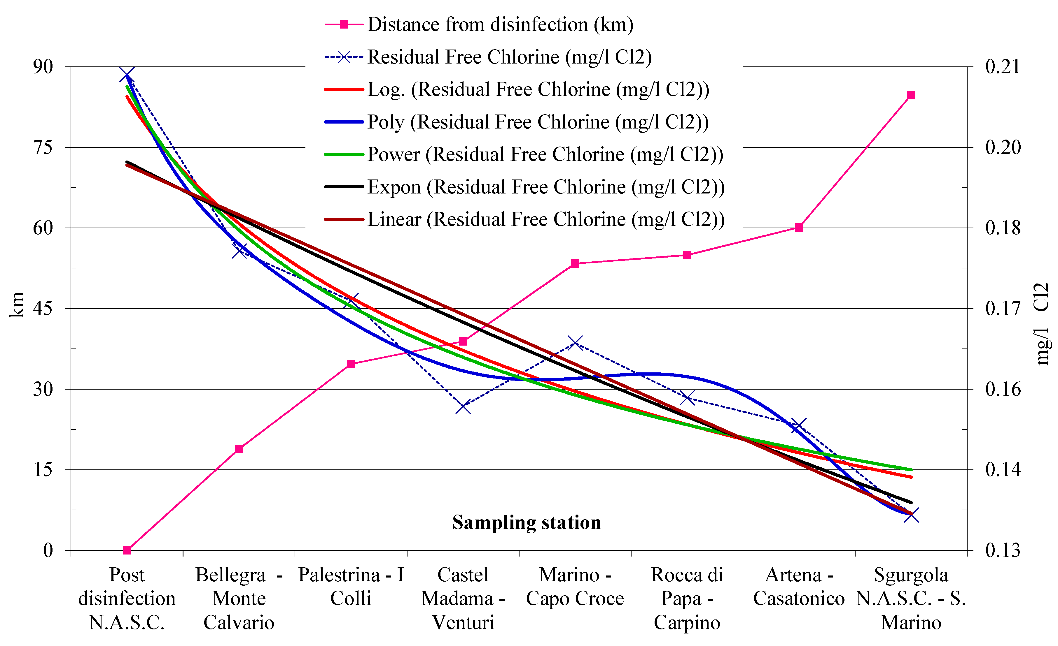
- The reduction of free chlorine is evident in the pipes closest to the origin of the aqueduct and in the pipes with smaller diameters characterized by more extended running times.
- The applied calculation model EPANET showed a good ability to represent the processes of quality degradation in the pipes working in hydraulic stationary conditions.
- kb values varied between 0.1 and 0.3 day−1 and kw varied between 0.01 and 0.07 m day−1.
- The experience should be repeated in other similar contexts, with future studies also trying to use some additional key parameters, in order to test the generalizability of this study’s findings to other similar situations.
Acknowledgments
Conflicts of Interest
References
- Storey, M.V.; van der Gaag, B.; Burns, B.P. Advances in on-line drinking water quality monitoring and early warning systems. Water Res. 2011, 45, 741–747. [Google Scholar] [CrossRef] [PubMed]
- Katsoyiannis, I.A.; Gkotsis, P.; Castellana, M.; Cartechini, F.; Zouboulis, A.I. Production of demineralized water for use in thermal power stations by advanced treatment of secondary wastewater effluent. J. Environ. Manag. 2017, 190, 132–139. [Google Scholar] [CrossRef] [PubMed]
- Hua, R.; Zhang, Y. Assessment of water quality improvements using the hydrodynamic simulation approach in regulated cascade reservoirs: A Case Study of drinking water sources of Shenzhen, China. Water 2017, 9, 825. [Google Scholar] [CrossRef]
- Yang, Y.J.; Haught, R.C.; Goodrich, J.A. Real-time contaminant detection and classification in a drinking water pipe using conventional water quality sensors: Techniques and experimental results. J. Environ. Manag. 2009, 90, 2494–2506. [Google Scholar] [CrossRef] [PubMed]
- Maslia, M.L.; Aral, M.M.; Ruckart, P.Z.; Bove, F.J. Reconstructing historical VOC concentrations in drinking water for epidemiological studies at a U.S. military base: Summary of results. Water 2017, 8, 452. [Google Scholar]
- Hall, J.; Zaffiro, A.; Marx, R.; Kefauver, P.; Krishnan, E.; Haught, R.; Herrmann, J. On-line water quality parameters as indicators of distribution system contamination. Am. Water Works Assoc. 2007, 99, 66–77. [Google Scholar]
- Sadiq, R.; Rodrssiguez, M.J. Disinfection byproducts (DBPs) in drinking water and predictive models for their occurrence: A review. Sci. Total Environ. 2004, 321, 21–46. [Google Scholar] [CrossRef] [PubMed]
- Łangowski, R.; Brdys, M.A. An Interval Estimator for Chlorine Monitoring in Drinking Water Distribution Systems under Uncertain System Dynamics, Inputs and Chlorine Concentration Measurement Errors. Int. J. Appl. Math. Comput. Sci. 2017, 27, 309–322. [Google Scholar] [CrossRef]
- Szabo, J.; Hall, J. On-line Water Quality Monitoring for Drinking Water Contamination. Compr. Water Qual. Purif. 2013, 2, 266–282. [Google Scholar]
- Munavalli, G.R.; Mohan Kumar, M.S. Water quality parameter estimation in a distribution system under dynamic state. Water Res. 2005, 39, 4287–4298. [Google Scholar] [CrossRef] [PubMed]
- Torretta, V. Environmental and economic aspects of water kiosks: Case study of a medium-sized Italian town. Waste Manag. 2013, 33, 1057–1063. [Google Scholar] [CrossRef] [PubMed] [Green Version]
- Tchobanoglous, G.; Schroeder, E.D. Water Quality; Addison-Wesley Publishing Company: Boston, MA, USA, 1992; p. 768. [Google Scholar]
- Hua, F.; West, J.R.; Barker, R.A.; Forster, C.F. Modelling of chlorine decay in municipal water supplies. Water Res. 1999, 33, 2735–2746. [Google Scholar] [CrossRef]
- Powell, J.C.; Hallam, N.B.; West, G.R.; Forster, C.F.; Simms, J. Factors which control bulk chlorine decay rates. Water Res. 2000, 34, 117–126. [Google Scholar] [CrossRef]
- Berry, D.; Xi, C.; Raskin, L. Microbial ecology of drinking water distribution systems. Curr. Opin. Biotechnol. 2006, 17, 297–302. [Google Scholar] [CrossRef] [PubMed]
- Frateur, I.; Deslouis, C.; Kiene, L.; Levy, Y.; Tribollet, B. Free chlorine consumption induced by cast iron corrosion in drinking water distribution systems. Water Res. 1999, 33, 1781–1790. [Google Scholar] [CrossRef]
- Wang, H.; Masters, S.; Edwards, M.A.; Falkinham, J.O.; Pruden, A. Effect of disinfectant, water age, and pipe materials on bacterial and eukaryotic community structure in drinking water biofilm. Environ. Sci. Technol. 2014, 48, 1426–1435. [Google Scholar] [CrossRef] [PubMed]
- Noma, Y.; Yamane, S.; Kida, A. Adsorbable organic halides (AOX), AOX formation potential, and PCDDs/DFs in landfill leachate and their removal in water treatment processes. J. Mater. Cycles Waste Manag. 2001, 3, 126–134. [Google Scholar]
- Katsoyiannis, I.A.; Hug, S.J.; Ammann, A.; Zikoudi, A.; Hatziliontos, C. Arsenic speciation and uranium concentrations in drinking water supply wells in Northern Greece: Correlations with redox indicative parameters and implications for groundwater treatment. Sci. Total Environ. 2007, 383, 128–140. [Google Scholar] [CrossRef] [PubMed]
- Katsoyiannis, I.A.; Zouboulis, A.I. Use of iron- and manganese-oxidizing bacteria for the combined removal of iron, manganese and arsenic from contaminated groundwater. Water Qual. Res. J. Can. 2006, 41, 117–129. [Google Scholar]
- Proctor, C.R.; Hammes, F. Drinking water microbiology-from measurement to management. Curr. Opin. Biotechnol. 2015, 33, 87–94. [Google Scholar] [CrossRef] [PubMed]
- Lu, W.; Kiene, L.; Levi, Y. Chlorine demand of biofilms in water distribution systems. Water Res. 1999, 33, 827–835. [Google Scholar] [CrossRef]
- Douterelo, I.; Boxall, J.B.; Deines, P.; Sekar, R.; Fish, K.E.; Biggs, C.A. Methodological approaches for studying the microbial ecology of drinking water distribution systems. Water Res. 2014, 65, 134–156. [Google Scholar] [CrossRef] [PubMed]
- Niquette, P.; Servais, P.; Savoir, R. Impacts of pipe material on densities of fixed bacterial biomass in a drinking water distribution system. Water Res. 2000, 34, 1952–1956. [Google Scholar] [CrossRef]
- Volterra, L. Presenza e sopravvivenza di varie forme biologiche in acqua di rete (Presence and survival of various biological forms in the water network). Ambient. Risorse Salut. 1994, 3, 23–30. [Google Scholar]
- Servais, I.; Anzil, A.; Ventresque, C. Simple Method for Determination of Biodegradable Dissolved Organic Carbon in Water. Appl. Environ. Microbiol. 1989, 55, 2732–2734. [Google Scholar] [PubMed]
- Servais, P.; Billen, G.; Laurent, P.; Levi, Y.; Randon, G. Studies of BDOC and bacterial dynamics in the drinking water distribution system of the Northern Parisian suburbs. J. Water Sci. 1992, 5, 69–89. [Google Scholar] [CrossRef]
- Kaplan, L.A.; Reasoner, D.J.; Rice, E.W. A survey of BOM in U.S. drinking waters. Am. Water Works Assoc. 1994, 86, 121–132. [Google Scholar]
- Elshobargy, W.E.; Abu-Qdais, H.; Elsheamy, M.K. Simulation of THM species in water distribution systems. Water Res. 2000, 34, 3431–3439. [Google Scholar]
- Foxon, T.J.; McIlkenny, G.; Gilmour, D.; Oltean-Dumbrava, C.; Souter, N.; Ashley, R.; Butler, D.; Moir, J. Sustainability criteria for decision support in the UK water industry. J. Environ. Plan. Manag. 2002, 45, 285–301. [Google Scholar] [CrossRef]
- Kalbar, P.P.; Karmakar, S.; Asolekar, S.R. Selection of an appropriate wastewater treatment technology: A scenario-based multiple-attribute decision-making approach. J. Environ. Manag. 2012, 113, 158–169. [Google Scholar] [CrossRef] [PubMed]
- Torretta, V. The sustainable use of water resources: A technical support for planning. A case study. Sustainability 2014, 6, 8128–8148. [Google Scholar] [CrossRef] [Green Version]
- Trulli, E.; Torretta, V.; Rada, E.C.; Istrate, I.A.; Papa, E.A. Modelling for use of water in agriculture. Agric. Eng. 2014, 44, 121–128. [Google Scholar]
- Aydin, N.Y.; Zeckzer, D.; Hagen, H.; Schmitt, T. A decision support system for the technical sustainability assessment of water distribution systems. Environ. Model. Softw. 2015, 67, 31–42. [Google Scholar] [CrossRef]
- Rossman, L.A. Epanet 2, User’s Manual; EPA/600/R-00/057, September 2000; Water Supply and Water Resources Division, National Risk Management Researh Laboratory, Office of Research and Development, U.S. Environtal Protection Agency: Cincinnati, OH, USA, 2000. [Google Scholar]
- Rossman, L.A.; Boulos, P.F. Numerical methods for modeling water quality in distribution systems: A comparison. J. Water Res. Plan. Manag. 1996, 122, 137–146. [Google Scholar] [CrossRef]
- Ohara, Z.; Ostfelda, A.; Lahava, O.; Birnhacka, L. Modelling heavy metal contamination events in water distribution systems. Procedia Eng. 2015, 119, 328–336. [Google Scholar] [CrossRef]
- Kiene, L.; Lu, W.; Levi, Y. Relative importance of the phenomena responsible for chlorine decay in drinking water distribution systems. Water Sci. Technol. 1998, 38, 219–227. [Google Scholar]
- Zhu, Z.; Wu, C.; Zhong, D.; Yuan, Y.; Shan, L.; Zhang, J. Effects of pipe materials on chlorine-resistant biofilm formation under long-term high chlorine level. Appl. Biochem. Biotechnol. 2014, 173, 1564–1578. [Google Scholar] [CrossRef] [PubMed]
- Notter, R.H.; Sleicher, C.A. The eddy diffusivity in the turbulent boundary layer near a wall. Chem. Eng. Sci. 1971, 26, 161–171. [Google Scholar] [CrossRef]
- UNICHIM. Metodologie di Analisi Delle Acque (Water Analysis Methodology) 2014. Available online: http://www.unichim.it/index.php?n=Pubblicazioni.MetodiAcque (accessed on 3 November 2017).
- Douterelo, I.; Sharpe, R.L.; Boxall, J.B. Influence of hydraulic regimes on bacterial community structure and composition in an experimental drinking water distribution system. Water Res. 2013, 47, 503–516. [Google Scholar] [CrossRef] [PubMed]
- Olyaie, E.; Banejad, H.; Chau, K.-W.; Melesse, A.M. A comparison of various artificial intelligence approaches performance for estimating suspended sediment load of river systems: A case study in United States. Environ. Monit. Assess. 2015, 187, 189. [Google Scholar] [CrossRef] [PubMed]
- Wang, W.C.; Xu, D.M.; Chau, K.-W.; Lei, G.J. Assessment of river water quality based on theory of variable fuzzy sets and fuzzy binary comparison method. Water Res. Manag. 2014, 28, 4183–4200. [Google Scholar] [CrossRef]


| Sampling Stations | Median | 70% | 80% | 90% | Min. | Max. | Average | Total Number of Samples | Yearly Number of Samples |
|---|---|---|---|---|---|---|---|---|---|
| Trevi, Hydraulic gallery, downstream of disinfection km 0 + 000 m | 0.2 | 0.23 | 0.24 | 0.25 | 0.1 | 0.29 | 0.21 | 90 | 41.5 |
| Bellegra, Monte Calvario km 18.450 | 0.19 | 0.2 | 0.21 | 0.22 | 0.05 | 0.25 | 0.18 | 40 | 18.5 |
| Palestrina, I Colli km 32.805 | 0.17 | 0.2 | 0.2 | 0.22 | 0.08 | 0.23 | 0.17 | 39 | 18 |
| Castel Madama, Venturi km 32.750 | 0.16 | 0.18 | 0.18 | 0.2 | 0.05 | 0.23 | 0.15 | 39 | 18 |
| Marino, Capo Croce km 55.019 | 0.17 | 0.18 | 0.2 | 0.21 | 0.1 | 0.25 | 0.16 | 42 | 19.4 |
| Artena, Casotonico km 58.047 | 0.15 | 0.16 | 0.18 | 0.19 | 0.06 | 0.21 | 0.14 | 34 | 15.9 |
| Gorga, San Marino km 77.224 | 0.13 | 0.15 | 0.18 | 0.2 | 0.07 | 0.23 | 0.14 | 41 | 18.9 |
| Sampling Station | Chainage | Hydraulic Residence Time | Dimensionless Residence Time, t | Mean Velocity |
|---|---|---|---|---|
| m | day | day day−1 | m s−1 | |
| Trevi, downstream to disinfection | 0 | 0.000 | 0.000 | = |
| Bellegra, Monte Calvario | 18.450 | 0.153 | 0.189 | 1.400 |
| Monte Castellone | 20.900 | 0.174 | 0.216 | 1.389 |
| Palestrina, I Colli | 32.855 | 0.263 | 0.326 | 1.446 |
| Castel Madama | 36.750 | 0.295 | 0.366 | 1.442 |
| Marino, Capo Croce | 55.019 | 0.485 | 0.601 | 1.314 |
| Artena, Casatonico | 58.047 | 0.545 | 0.676 | 1.233 |
| Gorga, San Marino | 77.224 | 0.807 | 1.000 | 1.108 |
© 2018 by the authors. Licensee MDPI, Basel, Switzerland. This article is an open access article distributed under the terms and conditions of the Creative Commons Attribution (CC BY) license (http://creativecommons.org/licenses/by/4.0/).
Share and Cite
Torretta, V.; Tolkou, A.K.; Katsoyiannis, I.A.; Katsoyiannis, A.; Trulli, E.; Magaril, E.; Rada, E.C. Consumption of Free Chlorine in an Aqueduct Scheme with Low Protection: Case Study of the New Aqueduct Simbrivio-Castelli (NASC), Italy. Water 2018, 10, 127. https://doi.org/10.3390/w10020127
Torretta V, Tolkou AK, Katsoyiannis IA, Katsoyiannis A, Trulli E, Magaril E, Rada EC. Consumption of Free Chlorine in an Aqueduct Scheme with Low Protection: Case Study of the New Aqueduct Simbrivio-Castelli (NASC), Italy. Water. 2018; 10(2):127. https://doi.org/10.3390/w10020127
Chicago/Turabian StyleTorretta, Vincenzo, Athanasia K. Tolkou, Ioannis A. Katsoyiannis, Athanasios Katsoyiannis, Ettore Trulli, Elena Magaril, and Elena Cristina Rada. 2018. "Consumption of Free Chlorine in an Aqueduct Scheme with Low Protection: Case Study of the New Aqueduct Simbrivio-Castelli (NASC), Italy" Water 10, no. 2: 127. https://doi.org/10.3390/w10020127