Impact of a Programme for Water Affordability on Residential Consumption: Implementation of the “Programa Mínimo Vital de Agua Potable” in Bogotá, Colombia

Abstract

Affordability of services is a determinant for people’s level of access to water. In this study, we analyse the effect of a programme aimed at improving the affordability of water services on users’ water consumption. The programme was implemented in 2012 by the local government of the city of Bogotá, Colombia, intending to provide an essential “lifeline” volume of water to poor households free of charge. Our assessment was carried out with secondary data and used difference-in-difference estimators in a panel data analysis of a two-period sample: 2011 and 2014. The unit of analysis was defined based on the city’s administrative divisions and the socio-economic stratification of residences. Over the period analysed, beneficiaries’ household consumption increased, reaching per capita consumption levels closer to those of the upper strata of users. Results suggest that the programme contributes to increased consumption and equity among users.

1. Introduction

Water consumption can vary significantly from one region to another. Variables that determine use profiles for water are of different types (environmental, economic, political, and social) and can depend on the scale of space and time.

Residential water consumption constitutes the main demand for water at the municipal level in urban areas. In recent decades, water consumption of this type has become particularly relevant considering problems related to scarcity, use conflicts and variability, which are a consequence of dynamics occurring within cities and interactions between cities and their surrounding regions.

Residential demand for water has been studied with different objectives, such as for forecasting, estimation of price elasticity, analysis of factors determining consumption and user behaviour, among others [1,2,3,4,5]. Estimating residential demand for water is considered a requirement to plan for any policy on water. However, doing so can be problematic for a number of reasons: a lack of reliable data, such as prices paid for services and users’ socioeconomic characteristics, and suboptimal use information in the condition of panel data [6].

Among different types of analyses aimed at determining residential demand for water, the variables commonly considered relevant are mainly associated with price, income, the population’s demographic characteristics, characteristics of housing and households, and climate factors [1,3,4,7]. However, the variables included in such models depend on the purpose of the analysis, the method used and availability of information.

Usually, the models used to assess water demand include relevant variables that, to a significant degree, manage to explain heterogeneous behaviours in urban settings at the scale of time and space [7]. Such models are important to evaluate public reaction to different changes such as, for example, those in public policies or programmes.

Price and income are typically the most studied factors [7]. Attempts to understand consumers’ reactions to changes in prices have led to studies on behaviour in reaction to different tariff structures. In particular, estimating the magnitude with which demand changes according to variations in price, income and other relevant factors can be a central guideline for future policies [4,6,8].

Several studies mention the importance of income and price elasticity of services in relation to water demand [9]. In connection with this, Nataraj and Hanemann [10] argued that residential demand for water was sensitive to a marginal increase in price, while other studies have found little or no reaction in actual consumption when studied with respect to price and income [1]. For example, Renwick and Archibald [11] observed that price elasticity was greater in low-income households compared to high-income ones, and Hoffman et al. [12] observed the same behaviour where the resident was owner compared to rented households. Thus, water demand and water management are associated with significant economic and social components [5] that must be taken into consideration.

Some studies have revealed that low-income families show little sensitivity to price due to their consumption being associated mainly with basic necessities, while high-income groups do not react to the intentions of the tariff structure since the price does not manage to weigh on their consumption habits [11]. However, in an analysis of price elasticity for different income groups in the urban area of Cape Town, Jansen and Shulz [4] found that demand within high-income groups was relatively more sensitive to price when compared with low-income groups.

Charging for water supply services can achieve different purposes, but the main aim is to collect revenues needed to maintain the financial sustainability of those services. However, the tariff must also incorporate the fact that the resource in question is essential for human development and, thus, must be available to the public at an affordable price. Recognising water as a human right means that reasonable prices are required for water that is meant for domestic uses. Thus, one of the main motivations for low tariffs has been to facilitate access to drinking water services for people in conditions of poverty [13,14].

The effectiveness of tariffs and restrictive policies varies among different types of users [15] and depends on how they are structured and implemented [16].

The different tariff structures in existence, in spite of their attempts to improve access conditions for the least advantaged, quite often continue to restrict access to water in sufficient quantities for such families. This happens because the particular characteristics of those families or households are not actually taken into consideration. In such cases, demand for water can be associated with a number of factors, such as the number of individuals, number of children, persons with specific illnesses, frequent use of toilets (in case of diarrhoea or menstruation), emergencies or cultural practices, among others.

The challenge for governments when charging for services that provide individuals with access to essential goods is, in the case of water, finding the balance between the minimum volume required and a reasonable tariff that favours conservation of the resource and minimal conditions of dignity [14]. One model that has been adopted is to incorporate subsidy strategies into fees collected from the entire user base in order to ensure access to a minimum volume of water, free of charge, for families in vulnerable conditions (determined according to their economic situation).

Some authorities have opted to supply a certain volume of water that is considered essential for basic or essential needs free of charge. Such cases have been observed in South Africa, where 6 m³/month is provided per household, and in Chile, where 15 m³/month is provided per family in proven situations of vulnerability.

Smith and Green [17] concluded that a policy ensuring a free quantity of water meant to meet basic needs was, in fact, insufficient for the majority of low-income households in Msunduzi (South Africa), since the amounts needed by those households was greater than the specified quantity. Indeed, tariff policies do not always manage to attain their objectives. For this reason, it is important to study each policy’s effects—particularly reactions of the beneficiary population—in order to assess and improve their effectiveness.

This type of analysis is still scarce due to the difficulties involved in obtaining data on the socioeconomic characteristics of the public. For this reason, studies that analyse demand for water without incorporating such data are common [5].

In the case under analysis herein, since 2012, the residences classified in the two lowest socioeconomic strata in Bogotá, Colombia, have the right to 6m³ per month free of charge, provided by the local government as an essential minimum amount of water. This study presents an evaluation of the programme’s effect on beneficiaries’ water consumption.

This article is divided into five sections including the present introduction. Section 2 briefly describes the programme and the tendencies related to household consumption in the case study. Section 3 outlines the secondary data upon which the analyses were based as well as the comparative analyses of the established groups and models to assess the programme’s impact. Section 4 presents the results, interpretation and discussion of the associated implications. Section 5 summarises the final considerations of this study.

2. Case Study: Minimum Essential Potable Water Programme Implemented in Bogotá

Bogota is the capital of Colombia. Its population is estimated at 7.7 million inhabitants, approximately 16% of the country’s population. The Bogota Water and Sewerage Company (Empresa de Acueducto y Alcantarillado de Bogotá ESP), a public company belonging to the municipality, is the main authority responsible for providing these services. The company provides water to approximately 1.7 million users with service coverage of 99%.

In Colombia, residences are classified in six socioeconomic strata according to the characteristics of the housing and the conditions of its surroundings. 1 is the lowest stratum and 6 is the highest. All residences are classified with the purpose of applying Colombia’s established public service tariff regime, which is based on cross subsidies. The highest strata (5 and 6) are obliged to make solidarity payments to those in the lowest strata (1, 2 and 3). The three lowest strata receive these contributions as subsidies to their fixed tariff and to their first 20 m³ consumed per month, which was defined as the basic volume (until 2016). Stratum 4 represents the middle stratum and pays the tariff without disbursing additional contributions or receiving any subsidies.

Despite the existence of that subsidised tariff, since 2012, Bogota City Hall has provided a free minimum volume of water, considered an essential level, to families in unfavourable economic conditions. The programme was denominated “Essential Minimum Potable Water” (Mínimo Vital de Agua Potable—MVAP) and is part of the city’s measures to ensure the human right to water [18].

The volume established within the programme as “essential” was 6 m³/month/household for residential water supply and is based on the estimated requirement of a household with four individuals [19]. Decree n° 64 of 2012 established that a policy would be developed to make the MVAP programme a right of those in strata 1, 2 and 3 that the municipal administration would have to fulfil gradually and progressively. However, the programme was only applied to households with water supply service classified under socioeconomic strata 1 and 2, the lowest of the six strata used to classify the population.

The last update of water demand forecasting in Bogota contains an analysis of residential consumption behaviour between the years 2008 and 2013. In that period, it was observed that the rate of consumption slightly diminished within strata 4, 5 and 6. Consumption levels for stratum 3 were apparently stable in the latest years. Meanwhile, consumption in strata 1 and 2 presented stable rates, with the exception of 2013, in which consumption increased [20]. 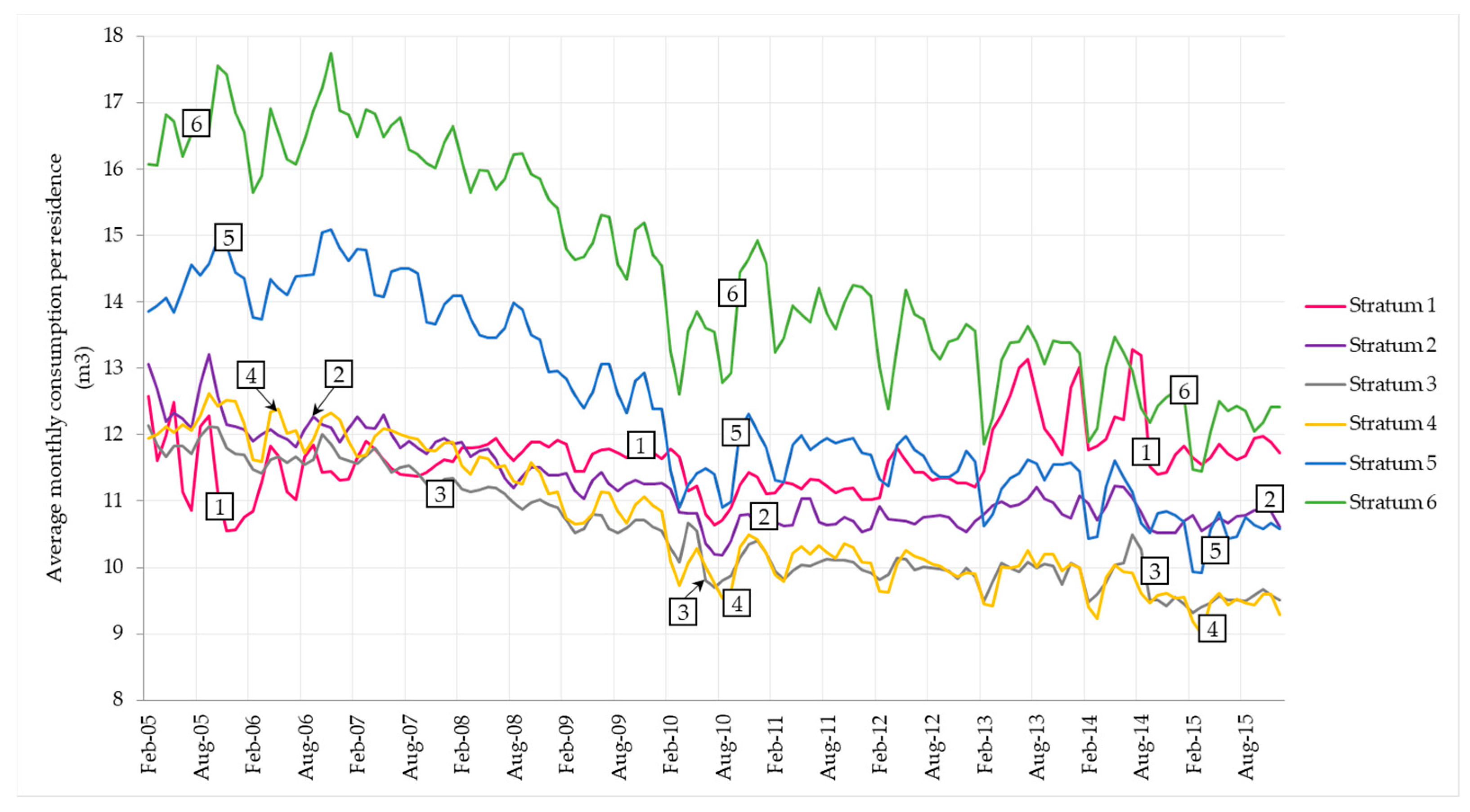Figure 1 represents average monthly consumption per household based on aggregated data per stratum and number of households, as per the service provider’s (Empresa de Servicios Públicos, ESP) reports to the Public Domestic Service Superintendence (SuperIntendencia de Servicios Públicos Domiciliarios, SSPD).

According to the study of water demand forecasting, one hypothesis that could explain the increase in consumption for the lowest socioeconomic strata in the year 2013 is that the MVAP programme was implemented in the first semester of 2012, between February and March [20]. On the other hand, in the same study, other possible explanations are mentioned: users from higher socioeconomic levels may have wanted to migrate to lower tariff brackets, and a subdivision of families may have occurred, starting in 2010, caused by an increase in construction and in household income.

3. Methods

3.1. Data Collection

In accordance with the objectives of this research, we referred to the dataset used to record bi-monthly billing information (consumption and rates, among others), exclusively for residential users, between 2009 and 2015. That information was provided by the water and sewerage company. Additionally, in an attempt to assess users’ socioeconomic profiles, we incorporated data from the Multipurpose Survey, applied in 2011 and 2014 on a random sample of Bogota’s population.

This data was obtained from the archive of the National Administrative Department of Statistics (Departamento Administrativo Nacional de Estadística, DANE) and was complemented with location data (neighbourhood level) provided by the District Planning Department of Bogota (Secretaría Distrital de Planeación, SDP). The Multipurpose Survey aims to collect socioeconomic information on the public for evaluation purposes and to follow up on action implemented by local governments.

Disaggregated information at the household level was available in each dataset. However, since some of that information was confidential, the responsible authorities omitted all data that could have been used to identify any individuals. For example, this includes information that could have been used to identify the household (address), which made any disaggregated analysis impossible at the household level.

Thus, common variables from both databases were used, consisting mainly in location and socioeconomic stratum. The common unit to identify location in both datasets was the neighbourhood. The residential stratification system within neighbourhoods was considered to check for the socioeconomic heterogeneity of households throughout neighbourhoods. Thus, in light of this, a neighbourhood-stratum category was created which was considered the unit of analysis in this study.

Availability of socioeconomic data before and after the application of the benefit was a determining factor to define the period over which the assessment would be carried out (the years 2011 and 2014). Another reason for selecting 2014 as the period subsequent to implementation was that it seemed to ensure sufficient time to guarantee users’ adaptation to the new condition. Thus, only units with information for both of those periods were considered. It is believed that data concerning users’ consumption after a period of two years since the programme’s implementation would reflect any changes that users would have adopted in their consumption habits. In that sense, the data analysis method adopted appears adequate to assess the programme’s effects on consumption.

Regarding the billing dataset, only households with consumption of an exclusively residential character and both water supply and sewage collection services were taken into account. Thus, households presenting inconsistencies with respect to stratum and services used over time were excluded. Billing data regarding consumption, prices paid, and discounts related to the programme benefit were used to calculate monthly averages for the period of one year. By considering the monthly average per year, changes in consumption related to seasonal factors were disregarded.

The data was from periods close to the point in time when the Multipurpose Survey was applied. In 2011, the Multipurpose Survey was applied between February and April 2011, and the period considered to estimate the monthly average consumption/amount spent per year, which depends on the household billing cycle, was between August 2010 and September 2011. In 2014, the Multipurpose Survey was applied between September and December of 2014, and the period considered to estimate the monthly average per year was between February 2014 and March 2015.

A single dataset was created by aggregating information per unit and subsequently combining common units from both datasets. The data taken into consideration allowed us to characterise the different units according to consumption, tariff paid for services and the population groups’ socioeconomic information.

3.2. Multiple Comparison Analysis

Two-way analysis of variance (ANOVA) with interaction was the test used to identify differences in consumption and prices paid between the different strata and periods, and the interaction between these two factors [21]. The assumptions of normality and homogeneity of variance of the residuals, which are used in two-way ANOVA, were tested through the Kolmogorov-Smirnov and Levene statistical tests, respectively.

For multiple comparison between the groups, the Tukey HSD test was used considering the Tukey-Kramer method for groups with different sample sizes [22]. The Tukey HSD test was selected given its robustness, its adequate control of total statistical significance, and its ability to compare groups with different sample sizes [23,24]. The Tukey HSD test with adjusted alpha was applied exclusively to comparisons of particular interest. Concretely, it was applied between the two periods for each stratum and, in each period, between all strata, in an attempt to check for a type I error present in pairwise comparison analyses owing to an inflated alpha. The tests were executed through the HSD.Tukey() function with adjusted alpha in R software’s Agricolae package [22].

Since the assumptions of the ANOVA were not completely satisfied, additional tests were applied to compare their outcome with that which was reached through the Tukey HSD test, attempting to confirm if this would generate problems in the result of the analysis. In this sense, the nonparametric Kruskal Wallis test was applied to the comparison between strata by period, as well as the Conover-Iman multiple comparison test with Bonferroni correction [25].

With respect to the comparisons between periods of strata, the ANOVA results were compared with those of the t-Student and Wilcoxon test with Bonferroni correction [25]. For all tests, a significance level of 10% was used. Because of the similar outcomes reached, the section on results and discussion (Section 4) only present the Tukey HSD test results.

Comparisons were performed for three scenarios: (i) considering all units, analysing the differences between the six strata and two periods; (ii) considering all units, analysing the differences between strata 1, 2 and 3 and the two periods; and (iii) considering only units of strata 1, 2 and 3 and the two periods. In the two latter cases, we attempted to identify the differences between strata with close socioeconomic characteristics.

3.3. Econometric Analysis

An econometric analysis of panel data was performed to assess the effects of the programme on users in the units under analysis, considering the same units before and after implementation of the programme. The difference-in-differences model was adopted, a quasi-experimental technique that measures the effect of an exogenous event on a particular period of time. This approximation depends on the presence of a treatment group (which is affected by the action) and a control group (which remains unchanged). Each group must include data at least from two periods or moments in time: one before the treatment (pre-treatment) and another after it (post-intervention), which allows systematic differences to be identified between the two groups. The model is defined by the following equation:

$${\mathit{Cons}}_{\mathit{it}}{=\beta }_0{+\beta }_1\times {\mathit{year}2014}_t{+\beta }_2\times {\mathit{MVAP}}_i{+\beta }_3\times \mathit{year}2014\times {\mathit{MVAP}}_{\mathit{it}}{+x}_{\mathit{it}}{\delta +\epsilon }_{\mathit{it}},$$

(1)

The independent variable ${\mathit{Cons}}_{\mathit{it}}$ represents the average monthly consumption per household in the unit i in year t. The variable ${\mathit{year}2014}_t$ was defined as a binary variable to represent the moment following the programme’s implementation. ${\mathit{MVAP}}_i$ was defined as a binary variable to indicate the treatment group, units with households that obtained the programme benefit (those classified in strata 1 and 2). $x_{\mathit{it}}$ represents a vector of the characteristics that change over time in the different aggregated units. ${\epsilon }_{\mathit{it}}$ is random error, which represents unobserved characteristics.

The difference-in-differences estimator, ${\beta }_3$ establishes the change in average consumption for those units of households that obtained the benefit. The Ordinary Least Squares (OLS) method was used to estimate the model’s parameters. A level of significance of 5% was used to analyse the results and the assumptions of the adjusted models were validated to determine the reliability of the results.

The traditional difference-in-differences estimator is based on strong assumptions, one of which is that the result of the averages for the samples of the treatment and control groups must follow a parallel pattern in the absence of an exogenous event [26].

Because of the common presence of heteroscedasticity in linear regression for panel and cross-sectional data, the presence of heteroscedasticity was estimated by the Breusch-Pagan test. The robust-standard errors were calculated in evidence of heteroscedasticity.

Stratum 3 was selected as the control group. The rationale behind this decision was that its socioeconomic level is closer to those of the programme beneficiaries (strata 1 and 2) and, thus, they would possess similar characteristics in comparison with the remaining strata. Moreover, in this stratum, consumption behaviour presented a parallel tendency in comparison to the two lowest strata during the years before the programme was implemented, as demonstrated in Figure 1 (see the period between 2009 and 2012). With respect to the tariff structure, they are also beneficiaries of a cross subsidy.

To select variables representing vector $x_{\mathit{it}}$, questions and answers from the socioeconomic surveys were chosen that corresponded with the variables reported in the literature on assessing residential demand for water in urban areas. In some cases, they were transformed into new variables per household since they correspond to disaggregated data per person or family within the household. Based on those variables, cluster analyses were performed to confirm correlation between the variables. Principal Component Analysis (PCA) was also carried out to maintain variables that would best represent correlated variables or substitute for a new variable calculated based on the former [27]. Furthermore, the significance of correlations between consumption and the variables was verified through Spearman’s rank correlation coefficient [21].

Finally, the Best Subset Regression method was used to avoid including irrelevant variables or to omit relevant variables in the difference-in-differences model. In this way, it was possible to determine a set of variables that best explained the behaviour of consumption in the linear regression. The method was executed using the regsubsets() function in R software’s Leaps package, which uses a branch-and-bound algorithm to perform an exhaustive search for the best groups of independent variables that predict the dependent variable in a linear regression [28]. Adjusted R-squared was used as the criteria to choose the models for best adjustment.

4. Results and Discussion

Table 1. Sample composition.

Strata	Units		Households
			Service Provider Utility		Multipurpose Survey
			2011/2014		2011		2014
	n	%	n	%	n	%	n	%
1	57	11.0	47,972	7.3	883	7.0	966	6.5
2	174	33.5	213,833	32.6	4585	36.5	4910	32.9
3	194	37.4	235,167	35.9	5096	40.6	6049	40.5
4	65	12.5	119,705	18.3	1542	12.3	2189	14.7
5	15	2.9	14,218	2.2	166	1.3	245	1.6
6	14	2.7	24,093	3.7	279	2.2	567	3.8
Total	519		654,988		12,551		14,926

represents the sample composition of 519 neighbourhood-stratum units. Those units were created by aggregating and combining data from billing and socioeconomic surveys datasets. The units are composed of a selection of households that represent approximately 42% of the total number of households. The socioeconomic characteristics attributed to each unit were composed of about 80% and 74% of the multipurpose surveys that were applied to random samples in 2011 and 2014, respectively.

4.1. Analysis of Water Consumption

Table 2. Statistical description of mean consumption (m³/household/month) per unit.

Period	Strata	Total	1	2	3	4	5	6
2011	Mean (Std Dv)	10.25 (1.91)	10.59 (1.68)	10.65 (2.07)	9.89 (1.67)	9.49 (1.92)	10.81 (1.92)	11.95 (1.55)
	Min	3.91	6.18	6.19	3.91	5.07	7.14	9.50
	Max	16.05	13.65	15.13	13.29	14.07	13.53	16.05
2014	Mean (Std Dv)	10.12 (1.98)	11.20 (1.73)	10.89 (2.10)	9.47 (1.58)	8.87 (1.66)	10.08 (1.82)	10.95 (1.44)
	Min	4.34	7.10	6.43	4.34	5.20	6.67	8.62
	Max	15.16	14.54	15.16	12.78	12.53	13.06	14.92
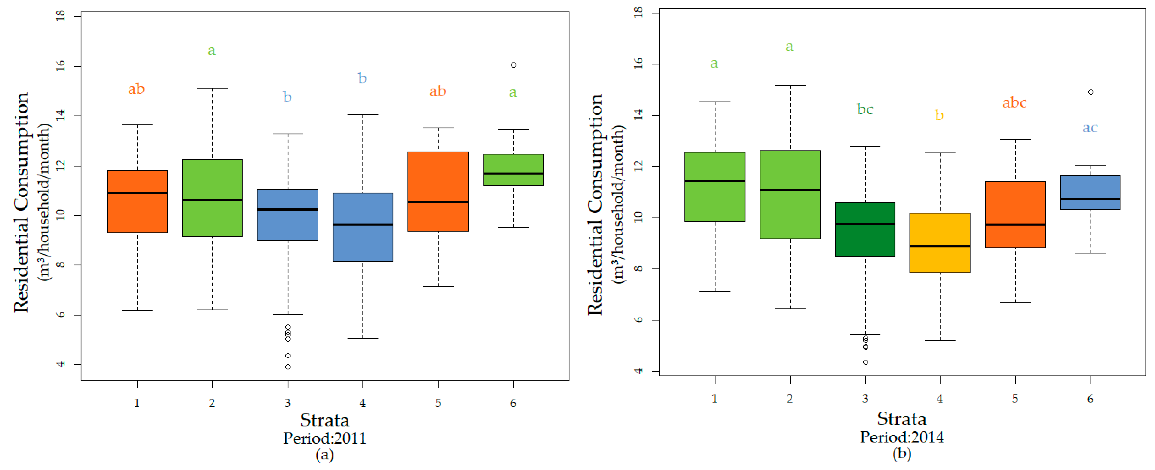
2011–2014		−0.135	0.611	0.240	−0.422	−0.617	−0.737	−1.000

presents descriptive statistics and differences between consumption means by unit per stratum, for both of the analysed periods. A tendency of reduced consumption per household can be observed in the latter years and, among all 519 units analysed, consumption in 2014 was slightly less than in 2011. However, when analysed by stratum, different tendencies emerge. For example, consumption increased for the beneficiary strata (1 and 2) and decreased for the remaining strata. Strata 3 and 4 present the smallest average levels of consumption per household, both in 2011 and 2014. Stratum 6 presents the greatest consumption level in 2011, but is surpassed by stratum 1 in 2014. The greatest difference (in absolute terms) in average levels of consumption between the two time periods under analysis was for stratum 6, while the least difference came from stratum 2. It is important to highlight that the findings for the sample of 519 units are coherent with the patterns presented in Figure 1 for all users of water services and the findings of the last study of water demand forecasting, which indicates that the sample adequately represents consumption behaviour within the scope of the study.

Upon comparing the different groups’ means of consumption, obtained through two-way ANOVA with interaction, considering the six strata, the hypothesis of equal averages among the different strata (p < 0.001) and between stratum:period interactions (p = 0.009) was rejected, indicating rather significant differences instead. The means between periods did not present significant differences (p = 0.2317). The same result, with regard to the significance level, was found when considering the dataset with only the first three strata. The significant stratum:period interaction suggests the importance of its effect on consumption and that such comparisons must be further explored, see Appendix A for further details. The results of the multiple comparison test for consumption are presented in

Table A1. Two-way ANOVA with interaction. Variable: Consumption per household.

Data Set	Factor	Df	Sum Sq	Mean Sq	F Value	Pr(>F)
Strata 1–6	Stratum	5	452.5	90.493	272.115	<2.2 × 10−16 ***
	Period	1	4.8	4.762	14.319	0.231739
	Stratum:Period	5	51.6	10.319	31.029	0.008707 **
	Residual	1026	3412.0	3.326
Strata 1–3	Stratum	2	264.72	132.362	392.619	<2 × 10−16 ***
	Period	1	0.03	0.031	0.0092	0.92363
	Stratum:Period	2	32.87	16.435	48.752	0.00785 **
	Residual	844	2845.34	3.371

Signif. codes: 0 ‘***’ 0.001 ‘**’ 0.01 ‘*’ 0.05 ‘.’ 0.1.

.

Figure 2 presents the result of the pairwise comparison analysis among strata, performed with the Tukey test, and shows mean consumption ± standard deviance of consumption for each stratum in the given year.

In Figure 2 different significances are presented with different letters (p < 0.1) between strata per year as follows: a = a, ab = a, ab = b, a < > b. For instance, considering all units (six strata), upon comparing mean consumption per household of units by stratum, in 2014, for the beneficiary strata, significant differences were noticed between strata 1 and 3 (p < 0.001), a < > bc, and 1 and 4 (p < 0.001), a < > b. These differences were not observed in the year 2011, ab = b. This can be explained by the magnitude in change between the years for these strata, in addition to the opposing tendencies regarding their consumption, while consumption increased in stratum 1, it decreased in strata 3 and 4, (see Table 2).

Other significant differences were found between strata 2 and 3 (p = 0.017, 2011, and p < 0.001, 2014), and 2 and 4 (p = 0.003, 2011, and p < 0.001, 2014) in both periods. Considering the dataset with only the three first strata, the same results were obtained except that the difference between strata 1 and 3 was significant in 2011 (p = 0.097) and 2014 (p < 0.001). The p-values of the pairwise comparison test of consumption are presented in

Table A2. Tukey’s Test. Variable: Consumption per household.

Interaction Stratum:Period	Difference of Means	p-Value 1
		i	ii	iii
2:2011-1:2011	0.06	14.999	3.000	2.924
3:2011-1:2011	−0.70	1.740	0.348	0.097
4:2011-1:2011	−1.10	0.179
5:2011-1:2011	0.23	14.972
6:2011-1:2011	1.37	1.812
3:2011-2:2011	−0.76	0.017	0.003	0.001
4:2011-2:2011	−1.16	0.003
5:2011-2:2011	0.17	14.991
6:2011-2:2011	1.31	1.544
4:2011-3:2011	−0.40	9.528
5:2011-3:2011	0.92	6.140
6:2011-3:2011	2.06	0.011
5:2011-4:2011	1.33	1.703
6:2011-4:2011	2.47	0.002
6:2011-5:2011	1.14	8.162
2:2014-1:2014	−0.31	13.127	2.625	1.528
3:2014-1:2014	−1.73	0.000	0.000	0.000
4:2014-1:2014	−2.33	0.000
5:2014-1:2014	−1.12	4.191
6:2014-1:2014	−0.24	14.966
3:2014-2:2014	−1.42	0.000	0.000	0.000
4:2014-2:2014	−2.02	0.000
5:2014-2:2014	−0.81	8.483
6:2014-2:2014	0.07	15.000
4:2014-3:2014	−0.60	2.964
5:2014-3:2014	0.61	12.225
6:2014-3:2014	1.48	0.587
5:2014-4:2014	1.21	2.855
6:2014-4:2014	2.08	0.024
6:2014-5:2014	0.88	11.832
1:2014-1:2011	0.611	1.110	0.222	0.228
2:2014-2:2011	0.240	3.290	0.658	0.668
3:2014-3:2011	−0.422	0.345	0.069	0.072
4:2014-4:2011	−0.617	0.810
5:2014-5:2011	−0.737	4.031
6:2014-6:2011	−1.000	2.205

Notes: ¹ Significant differences are in bold, n*p < 0.1, n = number of interest’s interactions considered in the bonferroni correction. Scenarios datasets: (i) Dataset strata 1–6 (n = 15, among strata by period, and n = 6, between both periods by stratum), (ii) Dataset strata 1–6, considering only interactions of strata 1–3, (n = 3, among strata by period, and n = 3, between both periods by stratum) (iii) Dataset strata 1–3, (n = 3, among strata by period, and n = 3, between both periods by stratum).

.

In the same test, when analysing differences between periods for each stratum, no significant differences were found for consumption, with the exception of stratum 3 (p = 0.069 and p = 0.072) in both cases where the higher strata were not considered in the analysis, (see Table A2).

Further elaborating on consumption behaviour per household,

Table 3. Average per capita consumption (L/inhabitant/day) and members per household per unit.

Period	Variable	Total	1	2	3	4	5	6
2011 1	Per capita consumption	104.0 (32.8)	85.4 (19.5)	95.7 (24.5)	99.5 (21.3)	126.0 (29.3)	150.5 (33.8)	193.3 (68.9)
	Members per household	3.48 (0.91)	4.25 (0.88)	3.83 (0.76)	3.41 (0.74)	2.60 (0.65)	2.50 (0.62)	2.24 (0.68)
2014 1	Per capita consumption	112.4 (29.0)	106.1 (27.3)	107.4 (27.1)	108.1 (24.2)	120.3 (16.7)	147.0 (33.4)	185.1 (31.2)
	Members per household	3.12 (0.73)	3.63 (0.61)	3.47 (0.59)	3.01 (0.62)	2.50 (0.57)	2.41 (0.78)	2.00 (0.24)
2011–2014 2	Per capita consumption	8.4	20.8	11.7	8.6	−5.7	−3.5	−8.3
	Members per household	−0.36	−0.62	−0.36	−0.41	−0.10	−0.09	−0.24

Notes: ¹ Mean and Standard Deviation in parentheses. ² Differences of means between 2011 and 2014.

presents average consumption per capita and the average number of members per household for each of the different units. A slight decrease was noted for consumption per household in 2011 and 2014, while a slight increase was apparent for per capita consumption. Per capita consumption patterns were not different in comparison to per household consumption in the different strata, except for stratum 3, for which an opposite tendency was observed with an increase in per capita consumption (see Table 2 and Table 3).

In this way, it is evident that analyses of consumption tendencies should consider the number of members per household. For both periods analysed, the number of members decreased as the stratum classification increased. The number of members per stratum were significantly different in strata 1, 2 and 3 between both periods studied (p < 0.001), while in the remaining strata those differences were not significant. Moreover, considering the dataset with only the three first strata, significant differences were found among the strata in both periods, except between strata 1 and 2 in 2014, as indicated by the p-values in

Table A3. Two-way ANOVA with interaction. Variables: Members per household.

Data Set	Factor	Df	Sum Sq	Mean Sq	F Value	Pr(>F)
Strata 1–6	Stratum	5	225.93	45.186	983.719	<2.2 × 10−16 ***
	Period	1	33.94	33.936	738.797	<2.2 × 10−16 ***
	Stratum:Period	5	5.09	1.017	22.143	0.05082 .
	Residual	1026	471.28	0.459
Strata 1–3	Stratum	2	62.81	31.405	657.581	<2 × 10−16 ***
	Period	1	36.71	36.708	768.627	<2 × 10−16 ***
	Stratum:Period	2	1.53	0.767	16.063	0.2012
	Residual	844	403.08	0.478

Signif. codes: 0 ‘***’ 0.001 ‘**’ 0.01 ‘*’ 0.05 ‘.’ 0.1.

and

Table A4. Tukey’s Test. Variables: Per capita consumption and Members per household.

Interaction Stratum:Period	Per Capita Consumption				Members Per Household
	Difference of Means	p-Value 1			Difference of Means	p-Value 1
		i	ii	iii		i	ii	iii
2:2011-1:2011	−0.31	1.337	0.267	0.044	0.43	0.008	0.002	0.001
3:2011-1:2011	−0.42	0.056	0.011	0.001	0.84	0.000	0.000	0.000
4:2011-1:2011	−1.22	0.000			1.66	0.000
5:2011-1:2011	−1.95	0.000			1.75	0.000
6:2011-1:2011	−3.24	0.000			2.01	0.000
3:2011-2:2011	−0.11	10.796	2.159	0.882	0.42	0.000	0.000	0.000
4:2011-2:2011	−0.91	0.000			1.23	0.000
5:2011-2:2011	−1.64	0.000			1.33	0.000
6:2011-2:2011	−2.93	0.000			1.59	0.000
4:2011-3:2011	−0.80	0.000			0.81	0.000
5:2011-3:2011	−1.53	0.000			0.91	0.000
6:2011-3:2011	−2.82	0.000			1.17	0.000
5:2011-4:2011	−0.73	0.173			0.10	14.937
6:2011-4:2011	−2.02	0.000			0.36	7.073
6:2011-5:2011	−1.29	0.002			0.26	13.628
2:2014-1:2014	−0.04	14.994	2.999	2.825	0.16	9.341	1.868	0.827
3:2014-1:2014	−0.06	14.939	2.988	2.560	0.63	0.000	0.000	0.000
4:2014-1:2014	−0.42	0.435			1.13	0.000
5:2014-1:2014	−1.22	0.000			1.22	0.000
6:2014-1:2014	−2.37	0.000			1.63	0.000
3:2014-2:2014	−0.02	14.997	2.999	2.863	0.46	0.000	0.000	0.000
4:2014-2:2014	−0.39	0.108			0.97	0.000
5:2014-2:2014	−1.19	0.000			1.06	0.000
6:2014-2:2014	−2.33	0.000			1.47	0.000
4:2014-3:2014	−0.37	0.180			0.50	0.000
5:2014-3:2014	−1.17	0.000			0.59	0.218
6:2014-3:2014	−2.31	0.000			1.01	0.000
5:2014-4:2014	−0.80	0.060			0.09	14.963
6:2014-4:2014	−1.94	0.000			0.50	1.785
6:2014-5:2014	−1.14	0.015			0.41	8.522
1:2014-1:2011	−0.62	0.000	0.000	0.001	0.62	0.000	0.000	0.001
2:2014-2:2011	−0.35	0.000	0.000	0.000	0.36	0.000	0.000	0.000
3:2014-3:2011	−0.26	0.014	0.003	0.002	0.41	0.000	0.000	0.000
4:2014-4:2011	0.17	3.053			0.10	6.192
5:2014-5:2011	0.11	10.616			0.09	10.863
6:2014-6:2011	0.25	5.877			0.24	5.147

Notes: ¹ Significant differences are in bold, n*p < 0.1, n = number of interest’s interactions considered in the bonferroni correction. Scenarios datasets: (i) Dataset strata 1–6 (n = 15, among strata by period, and n = 6, between both periods by stratum), (ii) Dataset strata 1–6, considering only interactions of strata 1–3, (n = 3, among strata by period, and n = 3, between both periods by stratum) (iii) Dataset strata 1–3, (n = 3, among strata by period, and n = 3, between both periods by stratum).

.

In comparison to the values observed in 2011, the values for per capita consumption in 2014 were closer among the lower strata, reaching values of 100 L/inhabitant/day (see Table 3). Per capita consumption per stratum was significantly different in strata 1, 2 and 3, between both periods studied (p < 0.001), while in the remaining strata those differences were not significant. Analysing the dataset with only the three first strata, significant differences were identified between per capita consumption in strata 1 and 2 (p = 0.044), and 1 and 3 (p < 0.001) in the year 2011, which were not statistically significant in the year 2014, (see Table A4 and

Table A5. Two-way ANOVA with interaction. Variables: Per capita consumption.

Data Set	Factor	Df	Sum Sq	Mean Sq	F Value	Pr(>F)
Strata 1–6	Stratum	5	272.41	54.482	922.315	<2.2 × 10−16 ***
	Period	1	16.41	16.414	277.872	1.651 × 10−7 ***
	Stratum:Period	5	13.32	2.663	45.087	0.0004528 ***
	Residual	1026	606.07	0.591
Strata 1–3	Stratum	2	5.14	25.712	48.760	0.007844 **
	Period	1	25.33	253.332	480.416	8.288 × 10−12 ***
	Stratum:Period	2	2.92	14.622	27.729	0.063052 .
	Residual	844	445.06	0.5273

Signif. codes: 0 ‘***’ 0.001 ‘**’ 0.01 ‘*’ 0.05 ‘.’ 0.1.

). The proximity of average per capita consumption between strata 1 and 2, and 1 and 3, in 2014, makes it possible to infer that greater equity was achieved with respect to access to a basic quantity of water.

Consumption levels were greater than the estimated value of 50 L/inhabitant/day, which is defined as the essential minimum volume by the government programme, and less than the values observed for higher strata. Per capita consumption in higher strata did diminish, but was still greater than 120 L/inhabitant/day and, thus, more than the levels of lower strata.

Howard and Bartram [29] provided estimates for different levels of service according to the type of access to water supply, the quantity of water consumed, the needs of individuals that were satisfied, and the level of health-related risk. Those authors considered that optimal access to water, meaning that which meets all domestic and hygiene-related needs and lowers health risks, would be that which provides an average quantity of at least 100 L/inhabitant/day, in specific conditions with continuous access from several sources located within a household. Given this, lower strata households can be considered to have reasonable consumption levels on the condition that their access is achieved through household connections with consistent water availability.

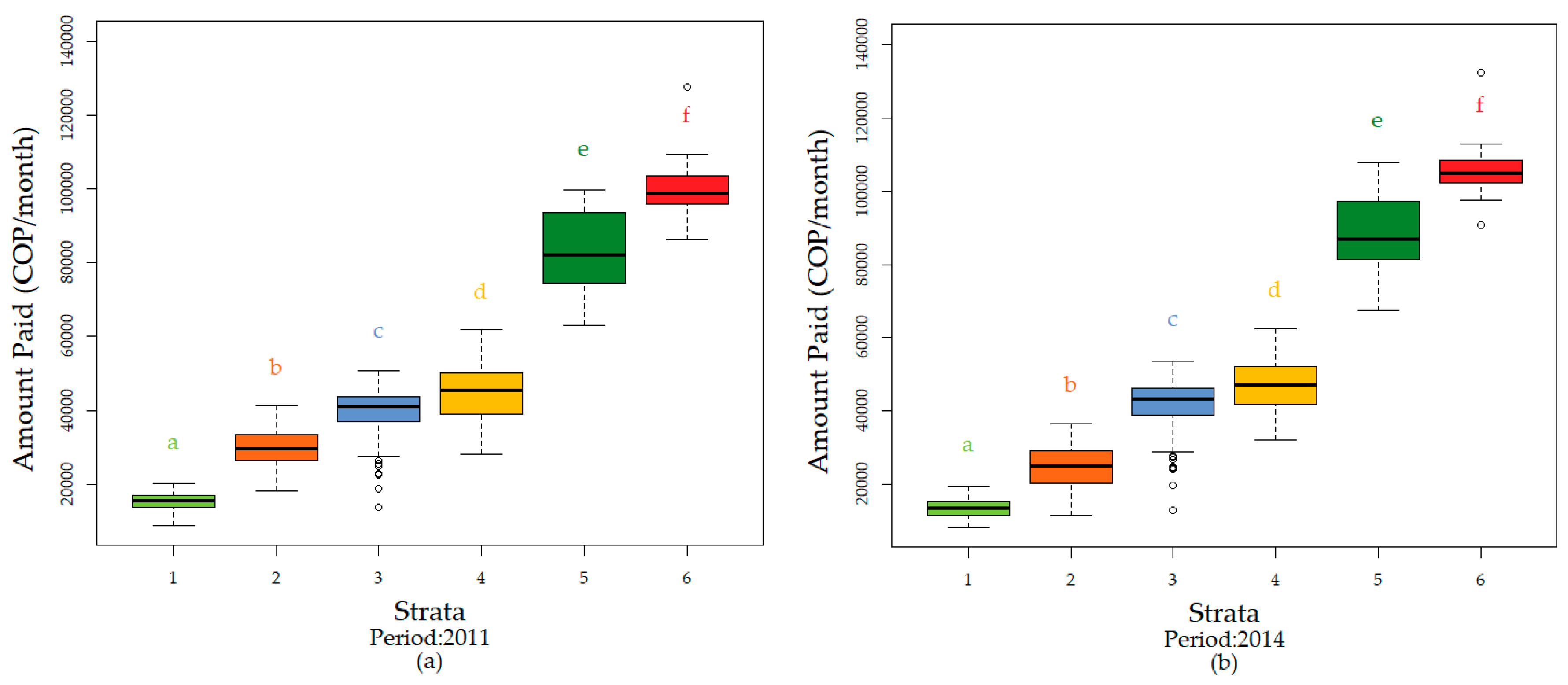
4.2. Analysis of Charges for Water and Sewerage Services

Table 4. Descriptive statistics of average monthly rates paid ($COP/month) per household in units.

Period	Strata	Total	1	2	3	4	5	6
2011	Mean (Std Dv)	37,211 (16,896)	15,234 (2299)	29,662 (4771)	39,832 (5765)	44,500 (7347)	83,669 (11,179)	100,580 (9630)
	Min	8708	8708	18,177	13,745	28,287	62,959	86,268
	Max	127,593	20,186	41,275	50,729	61,762	99,696	127,593
2014	Mean (Std Dv)	36,858 (19,393)	13,589 (2476)	24,785 (5356)	42,081 (6218)	47,084 (6979)	88,938 (11,490)	106,004 (9368)
	Min	8253	8253	11,475	13,158	32,270	67,627	90,654
	Max	132,300	19,535	36,577	53,743	62,530	107,872	132,300
Difference between means		−353	−1645	−4877	2249	2585	5270	5424

Notes: Values represented in Colombian Pesos (COP). Average exchange rate for the period studied in 2011: US$1 = COL$1831: in 2014: US$1 = COL$2104. Minimum wage 2011: COP 535,600; Minimum wage 2014: COP$616,000.

contains descriptive statistics of the amounts paid per household for water and sewerage services. The base fee as well as the charges for actual consumption were considered according to the tariff established for each stratum. The amounts paid in 2014 by strata 1 and 2 include the discount for their benefit from the MVAP programme. The increase in amounts paid can be considered a consequence of price readjustments by the Consumer Price Index (Índice de Precios al Consumidor, IPC) over time, considering that calculation methodology and tariff structure did not change in this period.

The same comparative analysis performed on consumption was also carried out on values paid by households. Through the two-way ANOVA with interaction test, significance differences were found among strata (p < 0.001) and among stratum:period interactions (p < 0.001). The means between periods did not present significant differences (p = 0.337). Considering the dataset with only the first three strata, the differences were significant between the periods (p < 0.001), among strata (p < 0.001) and, also, among stratum:period interactions (p = 0.001). The results of the multiple comparison test for the amount paid are presented in

Table A6. Two-way ANOVA with interaction. Variable: Amount Paid for water and sewerage services considering the programme discount.

Data Set	Factor	Df	Sum Sq	Mean Sq	F Value	Pr(>F)
Dataset Strata 1–6	Stratum	5	3.04 × 1015	6.07 × 1014	1733.346	<2.2 × 10−16 ***
	Period	1	3.23 × 1011	3.23 × 1011	0.9225	0.3371
	Stratum:Period	5	3.24 × 1013	6.47 × 1012	184.792	<2 × 10−16 ***
	Residual	1026	3.59 × 1014	3.50 × 1011
Dataset Strata 1–3	Stratum	2	7.43 × 1014	3.71 × 1014	1338.822	<2.2 × 10−16 ***
	Period	1	3.01 × 1012	3.01 × 1012	10.862	0.001023 **
	Stratum:Period	2	2.34 × 1013	1.17 × 1013	42.090	<2.2 × 10−16 ***
	Residual	844	2.34 × 1014	2.77 × 1011

Signif. codes: 0 ‘***’ 0.001 ‘**’ 0.01 ‘*’ 0.05 ‘.’ 0.1.

.

Significant differences were found in the pairwise comparison between strata (p < 0.001, for all comparisons) for both 2011 and 2014, see

Table A7. Tukey’s Test. Variables: Amount Paid without the programme discount and considering the programme discount for water and sewerage services.

Interaction Stratum:Period	Amount Paid (without MVAP)				Amount Paid (with MVAP)
	Difference of Means	p-Value 1			Difference of Means	p-Value 1
		i	ii	iii		i	ii	iii
2:2011-1:2011	14,428	0.000	0.000	0.000	14,428	0.000	0.000	0.000
3:2011-1:2011	24,598	0.000	0.000	0.000	24,598	0.000	0.000	0.000
4:2011-1:2011	29,266	0.000			29,266	0.000
5:2011-1:2011	68,435	0.000			68,435	0.000
6:2011-1:2011	85,346	0.000			85,346	0.000
3:2011-2:2011	10,170	0.000	0.000	0.000	10,170	0.000	0.000	0.000
4:2011-2:2011	14,838	0.000			14,838	0.000
5:2011-2:2011	54,007	0.000			54,007	0.000
6:2011-2:2011	70,918	0.000			70,918	0.000
4:2011-3:2011	4668	0.000			4668	0.000
5:2011-3:2011	43,837	0.000			43,837	0.000
6:2011-3:2011	60,748	0.000			60,748	0.000
5:2011-4:2011	39,169	0.000			39,169	0.000
6:2011-4:2011	56,080	0.000			56,080	0.000
6:2011-5:2011	16,911	0.000			16,911	0.000
2:2014-1:2014	15,633	0.000	0.000	0.000	11,196	0.000	0.000	0.000
3:2014-1:2014	24,014	0.000	0.000	0.000	28,492	0.000	0.000	0.000
4:2014-1:2014	29,003	0.000			33,496	0.000
5:2014-1:2014	70,857	0.000			75,350	0.000
6:2014-1:2014	87,923	0.000			92,416	0.000
3:2014-2:2014	8381	0.000	0.000	0.000	17,296	0.000	0.000	0.000
4:2014-2:2014	13,370	0.000			22,300	0.000
5:2014-2:2014	55,224	0.000			64,154	0.000
6:2014-2:2014	72,290	0.000			81,220	0.000
4:2014-3:2014	4989	0.000			4989	0.000
5:2014-3:2014	46,843	0.000			46,843	0.000
6:2014-3:2014	63,909	0.000			63,909	0.000
5:2014-4:2014	41,854	0.000			41,854	0.000
6:2014-4:2014	58,920	0.000			58,920	0.000
6:2014-5:2014	17,066	0.000			17,066	0.000
1:2014-1:2011	2848	0.156	0.031	0.012	−1645	2.072	0.414	0.287
2:2014-2:2011	4053	0.000	0.000	0.000	−4877	0.000	0.000	0.000
3:2014-3:2011	2263	0.003	0.001	0.000	2263	0.003	0.001	0.000
4:2014-4:2011	2585	0.197			2585	0.194
5:2014-5:2011	5270	0.227			5270	0.224
6:2014-6:2011	5424	0.234			5424	0.233

Notes: ¹ Significant differences are in bold, n*p < 0.1, n = number of interest’s interactions considered in the bonferroni correction. Scenarios datasets: (i) Dataset strata 1–6 (n = 15, among strata by period, and n = 6, between both periods by stratum), (ii) Dataset strata 1–6, considering only interactions of strata 1–3, (n = 3, among strata by period, and n = 3, between both periods by stratum) (iii) Dataset strata 1–3, (n = 3, among strata by period, and n = 3, between both periods by stratum).

. This result coincides with the fact that the tariff model for public services in Colombia is based on cross subsidies. Thus, contributions and subsidies are equal to a proportion of the established tariff’s value and are different according to the stratum and the rate paid. The proportion of subsidies and contributions established by the service provider for each stratum remained the same in the period between 2011 and 2014. In Figure 3, the result of comparisons (obtained via the multiple comparison Tukey test) between pairs per stratum are presented, showing the average ± the standard deviation of the values paid by each stratum per year.

Table 4 highlights the difference in values paid by each stratum in both periods. A reduction in the values paid by strata 1 and 2 can be observed, while values increased for all other strata. For the six strata and three strata dataset, there was a significant difference (p < 0.001) in mean values paid in the two periods for each stratum, except for stratum 1 (see p-values in Table A7). In part, this is probably explained by the benefit received by households in this stratum, which compensated for the increase in the tariff over the years studied. This same behaviour could be expected for stratum 2, since it also receives the benefit. However, there was a significantly lesser difference in average values paid between 2011 and 2014 for this stratum. This is explained by the fact that the programme ensures the same quantity of water free of charge to residences in both strata (6 m³) and, in accordance with the tariff structure, the value that strata 1 pays per m³ receives a 70% subsidy, compared to a subsidy of only 40% for strata 2. Thus, since stratum 2 pays a higher value per m³, the discount for 6 m³ of water is greater than what is received by households from stratum 1. For that reason, the difference in amount paid by stratum 2 (COP$4877) over the years that were studied was greater than the difference in amount paid by stratum 1 (COP$1645). In addition, results for the same comparison analysis for the amount paid in the scenario without the implementation of the programme are shown in Table A7 and

Table A8. Two-way ANOVA with interaction. Variable: Amount Paid for water and sewerage services without the programme discount.

Data Set	Factor	Df	Sum Sq	Mean Sq	F Value	Pr(>F)
Strata 1–6	Stratum	5	2.66 × 1015	5.32 × 1014	1513.600	<2 × 10−16 ***
	Period	1	2.56 × 1013	2.56 × 1013	72.842	<2 × 10−16 ***
	Stratum:Period	5	2.30 × 1012	4.60 × 1011	1.310	0.2573
	Residual	1026	3.60 × 1014	3.51 × 1011
Strata 1–3	Stratum	2	5.50 × 1014	2.75 × 1014	9859.621	<2 × 10−16 ***
	Period	1	2.01 × 1013	2.01× 1013	720.767	<2 × 10−16 ***
	Stratum:Period	2	1.49 × 1012	7.43 × 1011	26.657	0.07013 .
	Residual	844	2.35 × 1014	2.79 × 1011

Signif. codes: 0 ‘***’ 0.001 ‘**’ 0.01 ‘*’ 0.05 ‘.’ 0.1.

. In that case, the difference between the years for stratum 1 would be significant and the amounts paid for strata 1 and 2 would have increased as in the remaining strata.

Furthermore, average consumption levels for stratum 2 changed to a lesser extent in comparison to those of stratum 1. However, this comparison omits some variables that could have influenced those changes. For other strata, on the contrary, the values paid increased significantly. It may be highlighted that the tariff was not changed beyond the readjustments established by the IPC during the period that was studied.

The comparison of the selected units in both periods revealed a tendency in the latter years among households in the city of Bogota. The highest strata tended to consume lesser volumes, closer to the level of those consumed by the lower strata. This may be explained, in part, by the differences observed between the amounts paid by the averages of the highest and lowest strata in 2014, and by the reduced number of members per household.

Judging by the differences of the average amounts paid and consumption levels among the three lowest strata, it can be inferred that the changes in water consumption were due to the influence of the existing tariff structure and the possible effect of the MVAP being implemented since 2012. Yet, a more in-depth analysis is needed that incorporates demographic, social and economic variables in order to clarify the actual effect of the programme on beneficiaries’ consumption habits.

4.3. Estimation of the MVAP Programme’s Impact on Consumption

In an attempt to depict a consumption model to analyse the impact of the programme, certain information was selected from the Multipurpose Survey that could have some relationship with consumption habits. The variables taken into consideration encompassed the following categories: inhabitant characteristics, household characteristics, rational use practices and alternative water sources, and socioeconomic characteristics (see Appendix B for further details).

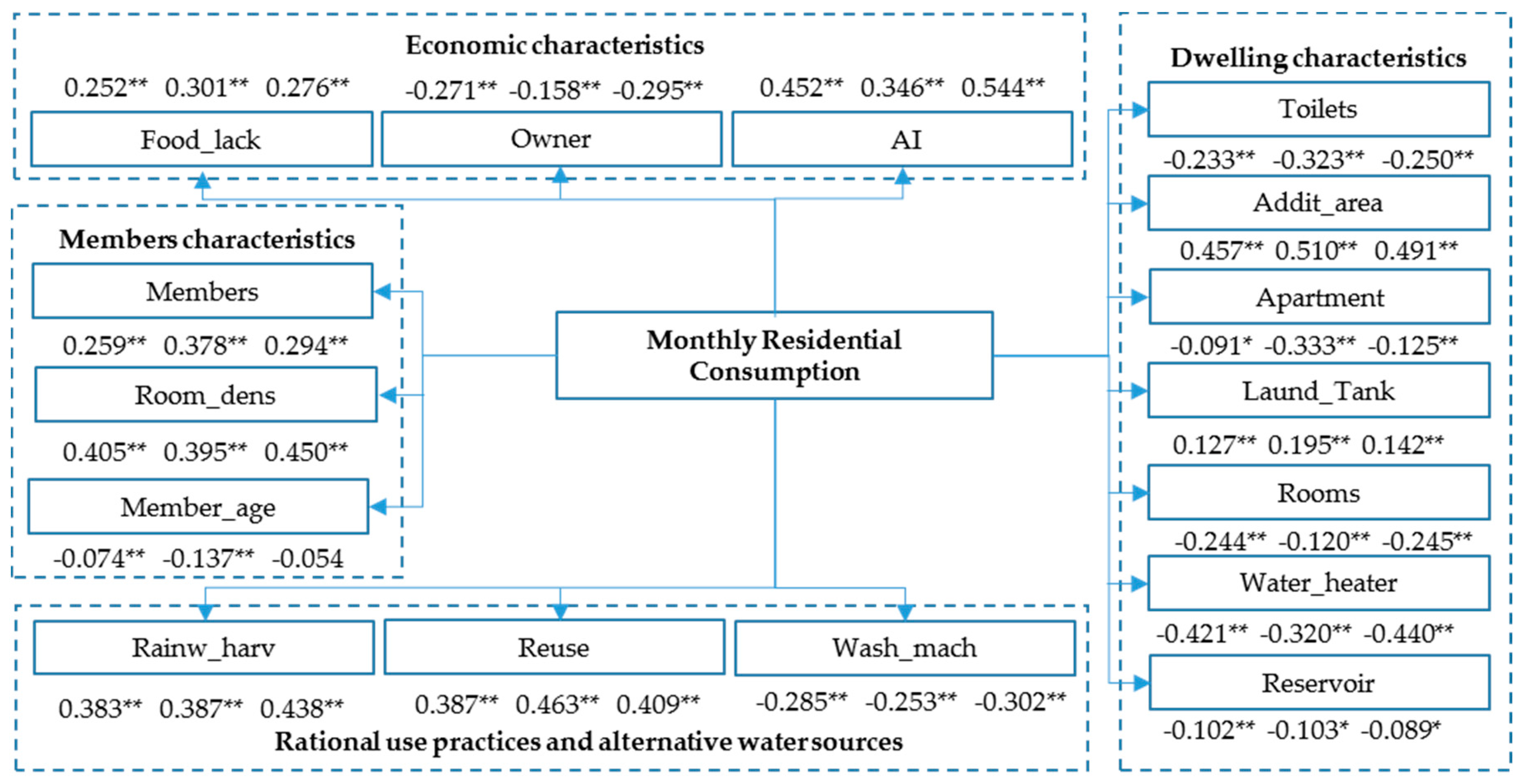
Figure 4 presents the Spearman coefficients $\left(\rho \right)$ of variables with greatest correlation to consumption, which were selected and created from three different datasets (scenarios), in accordance with the methodology: (a) strata 1, 2 and 3; (b) strata 1 and 3, and; (c) strata 2 and 3.

Based on the variables with greatest correlation to consumption, the Best Subset Regression model was used to select the variables. This method was implemented in several difference-in-difference models that were analysed in the present study.

The difference-in-difference models varied according to certain specifications: (i) control and treatment group; (ii) disaggregation of the strata, and; (iii) the variables included to identify changes in time.

Table 5. Specifications of the linear regression models.

Model	Treatment	Control	Control Variables
A	MVAP: Households with programme benefit (Classified in stratum 1 or 2).	E3: Stratum 3	Members, Owner, AI, Apartment, Addit_area, Laund_tank, Reuse
B	E1: Stratum 1 E2: Stratum 2		Members, AI, Apartment, Addit_area, Laund_tank, Reuse
C	E1: Stratum 1		Members, dom_dens, Owner, AI, Addit_area, Laund_tank, Reuse
D	E2: Stratum 2		Members, AI, Apartment, Addit_area, Laund_tank, Reuse

details each of the models. Appendix C presents the average and standard deviance of the variables selected to be a part of the models.

Table 6. Results of the difference-in-difference regression model.

Independent Variables	A	B	C	D	A.1	B.1	C.1	D.1
Year 2014_MVAP	0.589 **				0.592 **
	(0.191)				(0.192)
Year 2014_E1		0.789 *	0.610 *			0.676 *	0.632 *
		(0.307)	(0.310)			(0.300)	(0.307)
Year 2014_E2		0.606 **		0.554 **		0.546 **		0.545 **
		(0.208)		(0.206)		(0.207)		(0.206)
Year 2014	0.033	0.052	0.008	0.046	0.033	0.033	0.007	0.048
	(0.125)	(0.128)	(0.120)	(0.128)	(0.125)	(0.127)	(0.120)	(0.127)
MVAP	0.411 **				0.401 *
	(0.140)				(0.157)
E1		1.155 ***	1.178 ***			1.316 ***	1.241 ***
		(0.212)	(0.242)			(0.241)	(0.246)
E2		0.257 .		0.237		0.339 *		0.275 .
		(0.151)		(0.150)		(0.162)		(0.166)
Members	0.325 ***	0.315 ***	0.449 ***	0.311 ***	0.319 ***	0.388 ***	0.460 ***	0.344 ***
	(0.079)	(0.073)	(0.120)	(0.081)	(0.097)	(0.091)	(0.118)	(0.103)
Room_dens			−1.188 ***		0.039	−0.498 .	−1.158 ***	−0.198
			(0.358)		(0.278)	(0.283)	(0.349)	(0.329)
Owner	−0.013 ***		−0.013 **	−0.011 **	−0.013 ***	−0.013 ***	−0.011 **	−0.012 **
	(0.003)		(0.004)	(0.004)	(0.004)	(0.003)	(0.004)	(0.004)
AI	0.523 ***	0.735 ***	0.485 ***	0.612 ***	0.521 ***	0.680 ***	0.504 ***	0.630 ***
	(0.063)	(0.059)	(0.079)	(0.068)	(0.067)	(0.074)	(0.082)	(0.078)
Apartment	0.011 ***	0.016 ***		0.012 ***	0.011 ***	0.013 ***	0.004	0.012 ***
	(0.002)	(0.002)		(0.002)	(0.002)	(0.002)	(0.003)	(0.002)
Addit_area	1.651 ***	1.719 ***	1.021 ***	1.719 ***	1.655 ***	1.629 ***	1.132 ***	1.709 ***
	(0.183)	(0.182)	(0.208)	(0.186)	(0.183)	(0.179)	(0.223)	(0.186)
Laund_tank	0.028 ***	0.026 ***	0.030 ***	0.030 ***	0.028 ***	0.027 ***	0.030 ***	0.029 ***
	(0.006)	(0.005)	(0.006)	(0.006)	(0.006)	(0.005)	(0.006)	(0.006)
Reuse	0.016 ***	0.014 ***	0.016 ***	0.015 ***	0.016 ***	0.016 ***	0.016 ***	0.015 ***
	(0.004)	(0.004)	(0.004)	(0.004)	(0.004)	(0.004)	(0.004)	(0.004)
Constant	2.440 ***	1.276 *	4.271 ***	1.966 **	2.412 ***	2.310 ***	3.774 ***	2.095 **
	(0.600)	(0.559)	(0.588)	(0.635)	(0.619)	(0.604)	(0.685)	(0.654)
Ajusted R2	0.462	0.4734	0.4988	0.5002	0.4613	0.483	0.4999	0.4998
n	850	850	502	736	850	850	502	736
Residual Error	1.411	1.396	1.225	1.370	1.412	1.383	1.224	1.370
Residual Variance	1.991	1.949	1.501	1.877	1.994	1.913	1.498	1.877
Degrees of Liberty—Residuals	839	837	491	725	838	836	490	724
Number of variables	11	13	11	11	12	14	12	12

Notes: Robust-standard errors in parentheses, (.) p < 0.1, * p < 0.05, ** p < 0.01, *** p < 0.001.

contains the results of the difference-in-difference estimator for the different models’ specifications. In all models, stratum 3 was considered the control group given its similar behaviour to strata 1 and 2, both regarding consumption and socioeconomic characteristics. In this case, the difference-in-difference estimator is represented by the coefficient of variables for interaction between stratum and year, and depicts change in average consumption per household having obtained the benefit for units analysed.

The control variables that were considered over time for all models were: average number of additional areas per home, Addit_area; percentage of households with a laundry tank, Laund_tank; percentage of households with water reuse practices, Reuse; average rate of ability to pay in households ignoring the benefit, AI; and average number of household members, Members. Those variables had a significant effect on average consumption per household and are commonly used socioeconomic variables in models designed to assess demand for water.

An adequate adjustment level was obtained for the models that were developed in comparison with the results of other water consumption assessment models that incorporate socioeconomic variables [5]. When the treatment group corresponded with all of the programme’s beneficiaries, the adjusted model (A) managed to explain 46% of variance in the data. This number reached 50% when using adjusted models considering each stratum as treatment, separately, (C) and (D). Thus, given the different selected control variables for each model, according to the treatment group considered, the variables Room_dens, Owner and Apartment were not selected for all models. However, in an attempt to clarify their relevance and compare the several models for different treatment groups, all common control variables were included (models A.1, B.1, C.1 and D.1). It was found that the changes in variable coefficients and in the multiple determination coefficient, adjusted R-squared, were slight in comparison to the corresponding model that did not consider all variables.

Since the adjusted R-squared were similar among the adjusted models, models (C) and (D) were selected as those that best represented the cases under analysis, since the effect of the programme was considered separately for each stratum with the corresponding group of variables that adjusted the model best.

The results of the models suggest that the programme had a positive and significant effect on average consumption per household in the units that were studied. Estimated through model (C), which considers stratum 1 as treatment, the effect of the programme was 0.61 m³/month. For model (D), which considered stratum 2 as treatment, this figure was 0.554 m³/month. These results depend on the covariables remaining fixed. Thus, the programme’s impact on water consumption was slightly more in stratum 1 despite the discount being proportionately greater for stratum 2. It can thus be inferred that a direct relationship does not exist between the amount of the discount and consumption. In sum, a greater discount did not lead to greater consumption, contrary to what may have been expected. Therefore, it may be considered that the observed increases in consumption, corresponding with the effect of the programme, were related to basic levels of consumption per capita being attained rather than consumption increasing unreasonably. Indeed, in 2014, the three lowest strata presented similar average per capita consumption levels, as mentioned previously. Therefore, users did not necessarily react to lower tariffs for their services by wasting more water.

Jansen and Schulz [4] performed a study on the city of Cape Town (South Africa) to assess the factors that influenced water consumption. These authors observed that only 29% of households receiving water free of charge for consumption less than 6 m³/month, actually consumed the maximum allowed quantity.

Moreover, the coefficient values of the remaining variables evidence that the programme was not the main determinant for the consumption. The main difference between the specified models was the stratum variable’s effect and its significance, as may have been expected. Since strata 2 and 3 are closer than strata 1 and 3, the behaviour of the former was more similar. In the case of model (D), the stratum variable was not significant for the same reason: since the strata are close, the remaining variables explained the changes in consumption levels.

The constant was significant in both models and, similarly for the strata, the magnitude was greater in model (C) for the same reasons explained previously with respect to the stratum variable.

Other variables that presented a greater effect on consumption in comparison to the programme’s effect were, in the case of model (C): Room_dens and Addit_area; and in the case of model (D): Addit_area and AI. Additional variables with a lesser effect (nevertheless close to those of the programme) were, for model (C): AI and Members; and for model (D): Members. The year variable was not significant and the coefficient value was much less than that of previous variables, demonstrating its lacking influence on consumption in the periods studied. Among the remaining variables, Laund_tank, Reuse and Apartment, while significant, their effect on consumption was slightly less.

The programme did affect water consumption in the beneficiary strata despite the belief that low-income families are not overly sensitive to price given that their consumption is mainly for basic needs. Based on that observation, it can be inferred that the basic needs for water of the programme’s beneficiaries were not being met by the volumes that they consumed in 2011.

5. Conclusions

The analysis developed in the present study made it possible to identify a tendency of diminished consumption on the part of higher strata and increased consumption by lower strata over the specified period of time.

Research in the literature on assessments of water demand, predominantly, use economic instruments. Published works that adopt models integrating economic and social variables are rare due to the difficulties in obtaining data at the appropriate scales [30]. In the present analysis, despite the limitations, it was possible to assess the programme’s effect on average consumption of programme beneficiaries through secondary aggregate data by neighbourhood and stratum.

Judging from the results, it can be inferred that the programme had the effect of increased average consumption levels in beneficiary households in the units studied. An assessment of this type of social programme allows the actual effects of the said programmes to be clarified, when they incorporate other variables that simultaneously influence the behaviour of the variable under analysis, in this case water consumption.

Despite the existence of a socially differentiated tariff structure, which establishes subsidies and contributions according to socioeconomic conditions, per capita consumption in 2011 showed differences between strata that subsequently disappeared in 2014. Specifically, this was observed between the first three strata, evidencing improved conditions in terms of equity between those strata. Thus, it can be affirmed that the programme’s effect on consumption did not stimulate what could be considered excessive consumption.

The results obtained from the present analysis did not consider disaggregated data per household. For that reason, it was not possible to identify individual cases that could reflect extreme or atypical conditions in particular households. Moreover, studies encompassing a period of time after those analysed in the present research would be able to confirm the validity of the findings of the present study over time.