Return Level Estimation of Extreme Rainfall over the Iberian Peninsula: Comparison of Methods
by
Francisco Javier Acero
1,2,*, 
Sylvie Parey
3,
José Agustín García
1,2 and
Didier Dacunha-Castelle
4 1
Dpto. Física, Universidad de Extremadura, Avda. de Elvas s/n, 06006 Badajoz, Spain
2
Instituto Universitario de Investigación del Agua, Cambio Climático y Sostenibilidad (IACYS), Universidad de Extremadura, Avda. de Elvas s/n, 06006 Badajoz, Spain
3
Électricité de France/Recherche et Développement EDF/R&D, 6 Quai Watier, 78401 Chatou CEDEX, France
4
Laboratoire de Mathématiques, Université Paris 11, 91405 Orsay, France
*
Author to whom correspondence should be addressed.
Water 2018, 10(2), 179; https://doi.org/10.3390/w10020179
Submission received: 30 November 2017
/
Revised: 29 January 2018
/
Accepted: 2 February 2018
/
Published: 9 February 2018
(This article belongs to the Special Issue Selected Papers from the 1st International Electronic Conference on the Hydrological Cycle (ChyCle-2017))
Abstract
:Different ways to estimate future return levels (RLs) for extreme rainfall, based on extreme value theory (EVT), are described and applied to the Iberian Peninsula (IP). The study was done for an ensemble of high quality rainfall time series observed in the IP during the period 1961–2010. Two approaches, peaks-over-threshold (POT) and block maxima (BM) with the generalized extreme value (GEV) distribution, were compared in order to identify which is the more appropriate for the estimation of RLs. For the first approach, which identifies trends in the parameters of the asymptotic distributions of extremes, both all-days and rainy-days-only datasets were considered because a major fraction of values of daily rainfall over the IP is zero. For the second approach, rainy-days-only data were considered showing how the mean, variance and number of rainy days evolve. The 20-year RLs expected for 2020 were estimated using these methods for three seasons: autumn, spring and winter. The GEV is less reliable than the POT because fixed blocks lead to the selection of non-extreme values. Future RLs obtained with the POT are greater than those estimated with the GEV, mainly because some gauges show significant positive trends for the number of rainy days. Autumn, rather than winter, is currently the season with the heaviest rainfall for some regions.
1. Introduction
The precipitation regime in the Iberian Peninsula (IP) is highly variable due to its complex topography, for which reason no wide areas are left without coverage. The spatial variability of the IP rainfall is such that certain regions receive more than 3000 mm/year, while others, for example in the southeast, receive on average less than 200 mm/year, the lowest values in Europe. The atmospheric circulation patterns over the IP change depending on the season [1]. Although precipitation is generated by different physical processes during the different times of the year [2], the intensification of rainfall during the rainy seasons is due to frontal systems coming from the Atlantic Ocean [3,4], which cause persistent rainfall. For the eastern IP, rainfall is produced by easterly flows leading to heavy convective precipitation over the Mediterranean area, especially when there is colder air at high levels. Furthermore, over extensive regions of the IP, a few rainy days concentrate much of the annual precipitation [5]. This variability leads to a study of extreme rainfall over the IP being particularly interesting.
Previous extreme rainfall studies covering particular regions in Spain, the whole of Spain or the whole IP have considered a variety of indices, all taken from the Expert Team on Climate Change Detection and Indices (ETCCDI) set of indices recommended for use by the World Meteorological Organization [6]. For the region of Andalusia, among others [7], the most noteworthy results were found in winter, with a predominance of decreasing trends for intensity indices in central and western (CW) Andalusia, but positive trends in the south-eastern (SE) area. Another study of the whole IP [8] analyzed annual and seasonal trends of extreme precipitation indices using observations for Portugal and Spain and the ERA-driven simulation.
Some studies of extreme rainfall trends for the IP have used the statistical extreme value theory (EVT) and some the block maxima (BM) [9] or the peaks-over-threshold (POT) approaches [10,11]. These methods each have advantages and disadvantages, and it is important to compare the results they give. Recently, a new method has been developed for the calculation of non-stationary return levels (RLs) for extreme rainfall in a southwestern region of the IP [12]. The aim of this present study was not to propose a method to estimate the Rls, but to compare two ways of dealing with possible trends in rainfall so as to estimate near-future extremes. This objective is tackled for a set of complete daily rainfall time series from 76 gauges over the period 1961–2010 for the whole IP.
2. Data
The study area was the Iberian Peninsula. Most of the time series were taken from an extensive database of daily rainfall time series provided by the Spanish National Meteorology Agency (In Spanish: Agencia Estatal de METerología, AEMET). The quality requirements were to choose time series with no missing data and to cover the orographic diversity of the IP.
The final choice was a set of 76 daily rainfall time series (Table 1) corresponding to gauges as regularly spaced as possible over the IP. Their locations are shown in Figure 1. The study period was 1961–2010. Most of the time series were selected from the daily rainfall time series of AEMET according to the quality requirements described above. Four of the series were provided and quality controlled by the European Climate Assessment and Dataset service (ECA, available online at http://eca.knmi.nl), and one series was from Portugal (Gafanha da Nazaré) provided by the National System of Water Resources Information (SNIRH, available online at http://snirh.apambiente.pt/, managed by the Portuguese Institute for Water) database.
It is often important to determine whether a set of data is homogeneous before any statistical technique is applied to it. Inhomogeneities in long-term climatological time series could be due to various factors, such as changes in instruments, observation methods, station relocation, etc. Data homogeneity was evaluated using the R-based program RHTestV3, developed at the Climate Research Branch of the Meteorological Service of Canada, and available from the ETCCDI, Expert Team on Climate Change Detection and Indices website (http://etccdi.pacificclimate.org/). This program is capable of identifying multiple step changes at documented or undocumented change-points. It is based on a two-phase regression model with a linear trend for the entire base series [13,14]. This analysis, together with the metadata of the stations showed that none of the 76 time series had change-points significant at 5%, with all of them being homogeneous in the cited period of study.
For this study of extreme precipitation over the IP, in view of the highly seasonal nature of rainfall, each season was studied separately. The definition of the seasons used was that common in climatological studies: winter was December, January and February; spring was March, April and May; and autumn was September, October and November. Summer was not considered because of the low number of rainy events during that season in most parts of the IP. For the BM approach, each season was considered for the selection of its maximum value. For the POT approach, the threshold used in defining extreme rainfall for each season separately was the 98th percentile of all the daily rainfall values for the whole period and the 95th percentile of the rainy-days-only values.
3. Methods
The 20-year RLs for the precipitation in the IP were studied using two different EVT approaches—the BM and the POT—considering both all-days (rainy and non-rainy) and rainy-days-only datasets. The BM approach is frequently applied to the study of extreme events of meteorological variables in the framework of EVT. Its focus is on modeling the BM of the variables with the generalized extreme value (GEV) distribution. The GEV theory is a kind of “law of large numbers”. It states that the maximum of n independent and identically distributed variables with probability distribution function of type F tends to follow a GEV distribution when n tends to infinity (i.e., in practice, for large enough n).
In a similar way, the POT approach is based on the asymptotic convergence of the exceedances of a high threshold u to a general Pareto distribution (GPD) when u tends to infinity. This holds true again for independent and identically distributed variables.
Making an optimal choice for the threshold u is a difficult problem. A very high value of u leads to few exceedances and consequently high variance estimators. On the contrary, a very low value of u is likely to violate the asymptotic basis of the model, leading to biases [15].
An independent and identical distribution is assumed by the theory, but is generally not verified for meteorological variables. Weak dependence can be dealt with: annual maxima can generally be considered as independent, and values above the threshold can be made independent, for example by applying a run declustering procedure [16]. An identical distribution is not true because of seasonality, interannual variability and possible trends. To handle seasonality, estimations are made for each season rather than for the whole year. Interannual variability and trends are more difficult to tackle. The estimation of RLs in a non-stationary context has been the subject of a growing number of papers in recent years. While some authors consider that taking non-stationarity into account implies too large uncertainties to be justified [17,18], others suggest methods for doing so together with new definitions for an RL in such a context [19,20,21,22,23,24].
The objective of the present work was not to derive an RL for some design purpose, but to compare two ways of dealing with possible trends in rainfall when estimating near-future extremes. The focus was therefore not on the definition of a non-stationary RL, but on the type of trends to be considered and the consequences of the choice for both the BM and the POT approaches. Thus, two different approaches were used to compute future RLs:
- (1)
- The first consists of identifying trends in the parameters of the asymptotic distributions of extremes: location and scale parameters of the GEV for the BM and threshold and scale parameters of the GPD for the POT. The trend identification is based on likelihood ratio tests at a 5% significance level between models with linear or constant parameters [15], and the confidence intervals (CI) are computed by bootstrapping in order to take the uncertainty in the trends into account (see the Appendix in [12] for details).
- (2)
- A residual process that has been explained extensively elsewhere [12] is used in order to calculate the 20-year RLs for 2020. The idea is to use trends in the main characteristics of the whole distribution rather than those in the extreme values only. If the non-stationarity of extremes in a statistical framework is explained by means and variances, the daily mean and standard deviation in 2020 are estimated by linear extrapolation of the linear trends that have been estimated from observations so as to be able to compute the RLs for 2020.
Although linear trends are poorly suited to represent future evolutions in rainfall correctly, they were chosen here as a simple way to compare two different approaches under similar conditions. The second approach is appropriate for the use of climate simulation results to compute future means and standard deviations and is preferable if the aim is to estimate future RLs as design values for an installation or project.
4. Results
This section presents the main results of the 20-year RL (Z20) estimations. The present day was estimated using both all-days (Section 4.1) and rainy-days-only (Section 4.2) data, and the near future was estimated for 2020 (Section 4.3).
4.1. Present 20-Year RLs Estimated from All-Days Rainfall Data
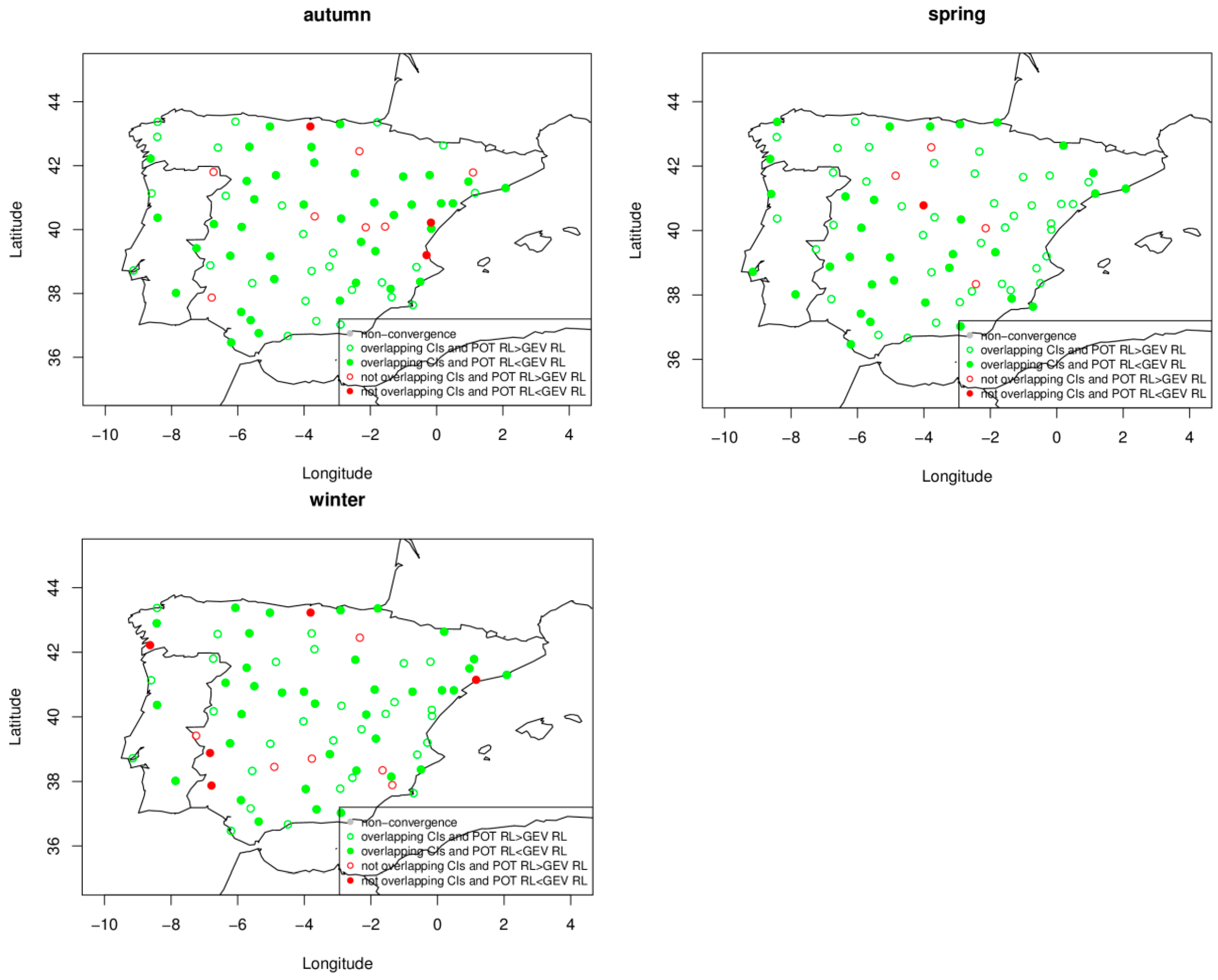
Considering all days (rainy and non-rainy), the 20-year RLs for the two approaches were estimated for the present day by using the daily rainfall time series. Figure 2 shows the results for the three seasons considered. For autumn and spring, all the 20-year RLs estimated using the POT approach lay inside the CI of the 20-year RLs using GEV. In winter, only one gauge (vlm) showed no overlapping CIs, the RL estimated with the POT (55.09 [47.96; 62.22]) being greater than that corresponding to the BM (50.16 [45.51; 54.81]). The difference between the two values is small, but since the CI with BM is narrower than with POT, the RL estimated with the POT does not fall inside the GEV CI.
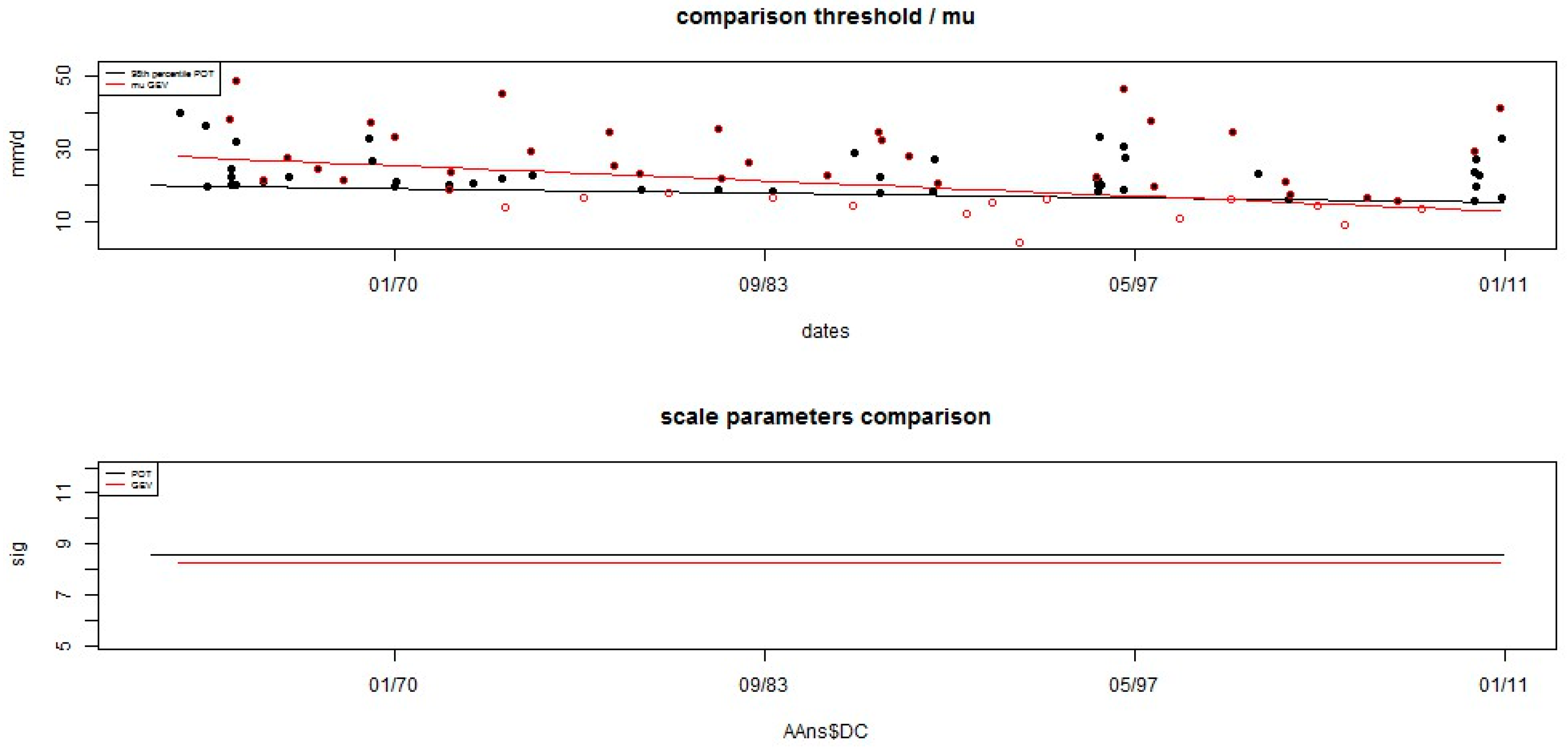
In order to further analyze this exception, Figure 3 shows the GEV/POT comparison for this gauge (vlm) in winter. Looking at the top figure, one observes that the frequency of threshold exceedances has decreased over the last decade, and the last values are lower than the rest. Considering the red points for GEV in greater detail, one sees that, as one maximum is chosen for each season, high and low values are mixed, some of them being lower than the POT threshold. The shape parameter is different: ξ = 0 for POT and ξ = −0.2845 for GEV. In this latter case, the distribution is strongly bounded, which is surprising for precipitation. Since sigma measures the variability, the scale parameter is greater in GEV because the maximum is more variable than in POT when choosing such low values as the maximum (a season with less than 10 mm of rainfall is not really a maximum). The estimates were made as if the time series were stationary, which is probably not the case and may further explain the differences.
4.2. Present 20-Year RLs Estimated from Rainy Days
Considering rainy-days-only and studying when Z20-POT is inside the CI of Z20-GEV, we show in Figure 4 the results for the three seasons considered. For both autumn and winter, all the gauges except one in each case (pcr and cal, respectively) have Z20-POT inside the Z20-GEV CI, and for spring, there are three exceptions (cal, gra, ssp). In all cases, Z20-POT is greater than Z20-GEV. The CI obtained using GEV is narrower than that corresponding to POT.
The gauges with non-overlapping CIs and different values for the RL present the same behavior. Figure 5 illustrates the GEV/POT comparison for the gauge “pcr” in autumn. There are many maxima in the second half of the study period with the BM approach, with low rainfall leading to smaller RL values.
4.3. Future 20-Year RLs
In this section, we shall present the main results of calculating the 20-year RLs for 2020. It is remarkable that, in a stationary context, according to the likelihood ratio test at a 95% confidence level, the value of the shape parameter is zero for most of the stations for all three seasons considered.
4.3.1. Using Trends in the Parameters
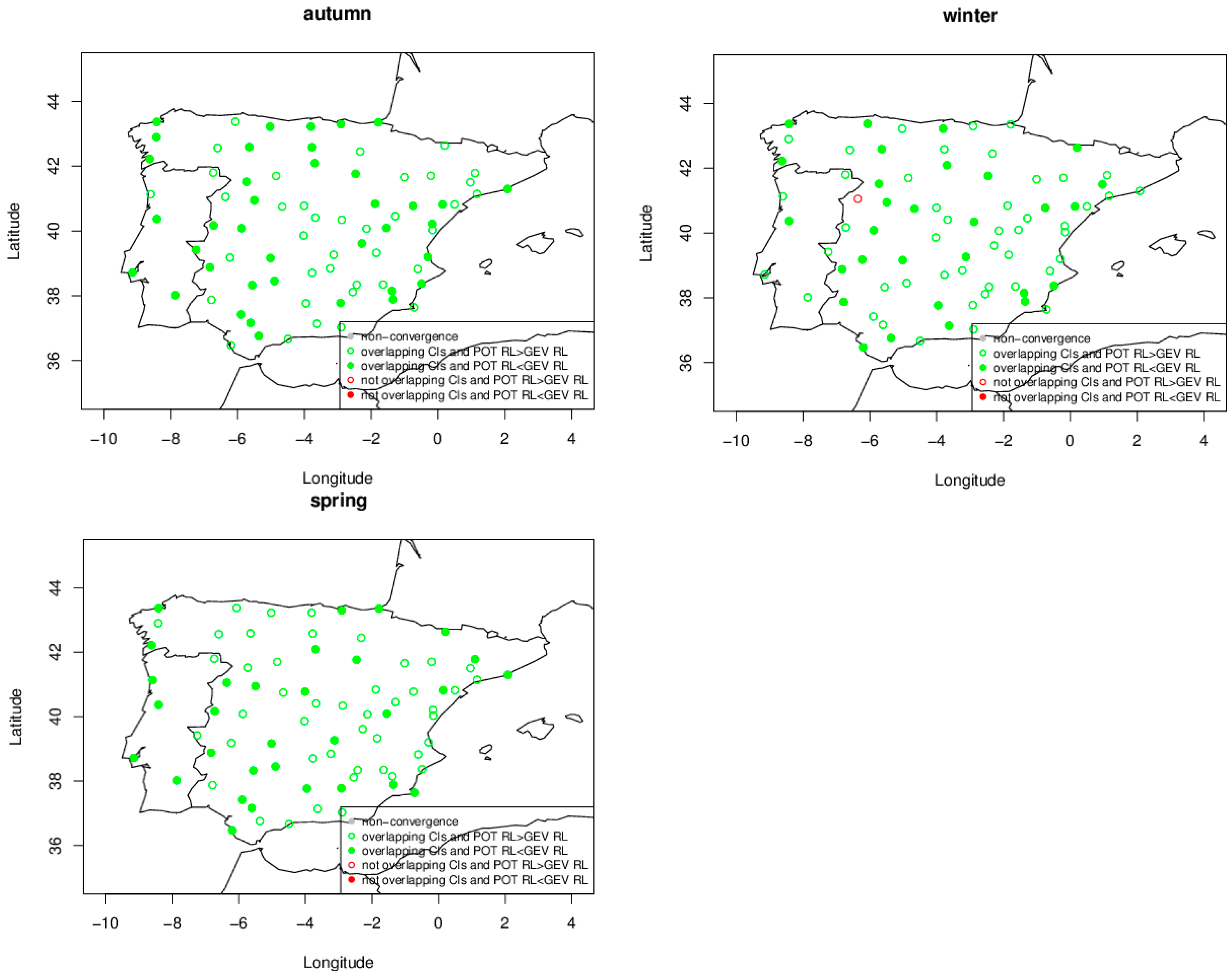
We first studied the future 20-year RLs obtained through extrapolating the trends in the parameters (scale and location for GEV and scale and threshold for POT), checking whether the RLs obtained with POT lay within the CI of the RLs obtained with GEV. Figure 6 shows the results. As can be seen, there are several gauges with non-overlapping CIs: 10 for autumn, 11 for winter and 5 for spring. For these gauges, Table 2, Table 3 and Table 4 list the degree of each parameter for GEV and POT, with zero meaning no trend and one a linear trend. Most of these gauges show discrepancies between the degree obtained for the parameters using the two methods; when there is a linear trend in the scale or location parameters using GEV, there is no trend in the scale parameter using POT, and vice versa. This leads to different values of the 20-year RL for 2020 as estimated by extrapolating the parameters.
Our consideration of a varying threshold for POT was roughly equivalent to considering a linear trend in the location parameter (μ) for GEV. Thus, those situations in which μ shows a linear trend, and σ for GEV and GPD shows no trend should be similar. The gauges that disagree (such as “agr”) may be a result of the sampling, because lower values are considered using the BM approach. By way of example, Figure 7 shows the behavior with the two approaches for the gauge “agr” in autumn.
Figure 8 shows the comparison of the two approaches for the gauge “dto” in winter. Again, the decrease in the location parameter is greater than that in the threshold due to the lower maximum values, especially in the second half of the time series. This leads to a lower value of Z20 for 2020 when using GEV than when using POT. The same is the case for the gauge “cal”.
4.3.2. Using the Stationarity Test
The next step is to estimate the 20-year RLs for 2020 obtained by extrapolating the linear trends in the daily mean and standard deviation of the amount of rain for rainy days and in the number of rainy days [12]. The hypothesis that the non-parametric temporal evolution is essentially linked to the evolutions of the mean and the variance (the methodological approach mentioned in [12]) had previously been used to test the stationarity of the extremes of standardized residuals of the time series. Table 5 shows the percentage of gauges that verified this stationarity at a 90% confidence level. The stationarity test was reasonably well satisfied by both methods: for the BM approach, 87% of the gauges satisfied the test in autumn and spring and a lower proportion, 78%, in winter; for the POT approach, greater proportions of gauges satisfied the test: 95% in autumn and spring and 92% in winter.
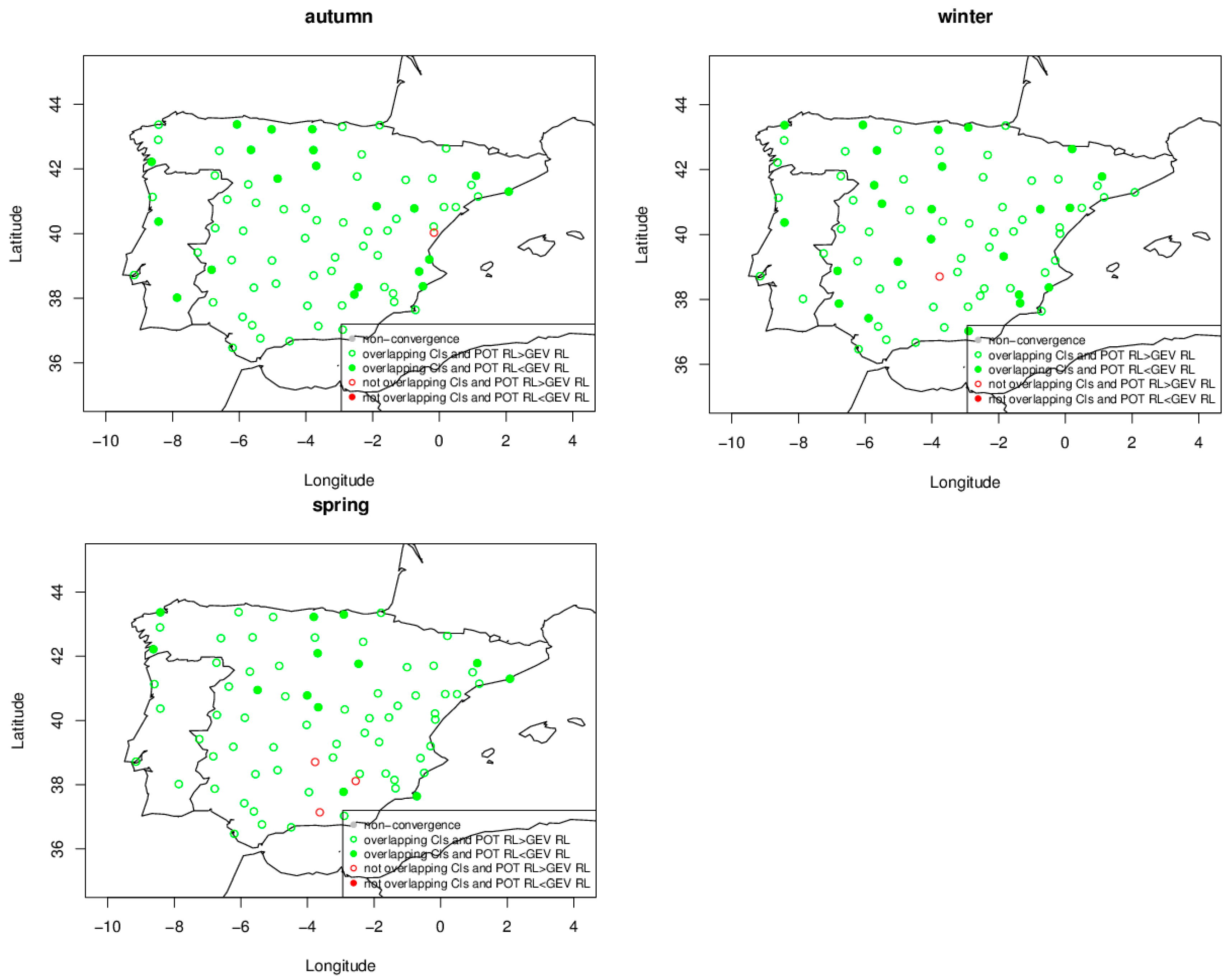
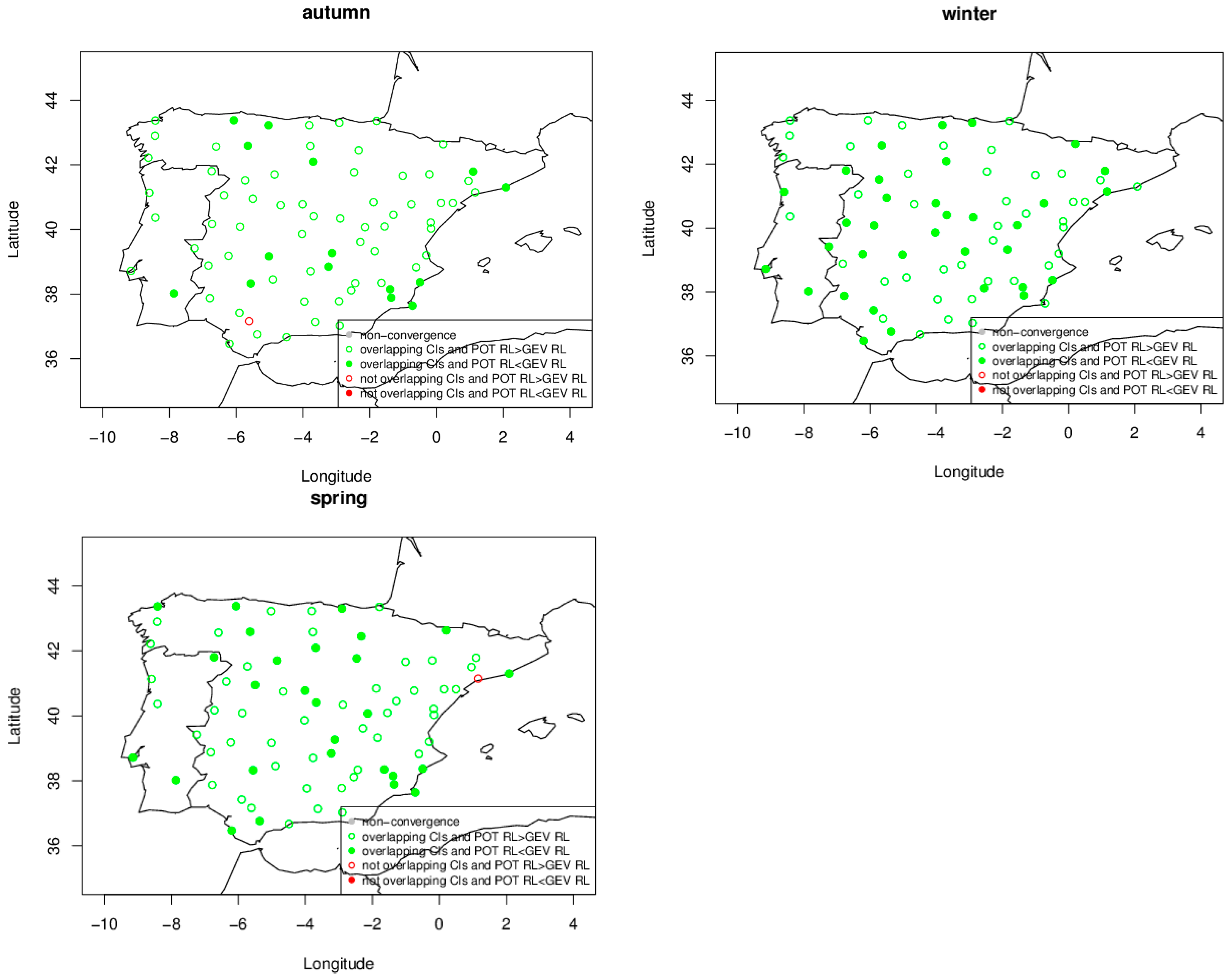
Having checked that the stationarity test is fairly well satisfied by both methods, we then estimated the 20-year RLs for 2020. Figure 9 shows the spatial distribution of the stations with an RL obtained with POT that was within the CI of the RL obtained with GEV. The comparison showed similar results for the two methods, giving overlapping CIs for all the gauges in winter, and all except one in both autumn and spring.
It should be noted that we did not extrapolate the trends in parameters, but the trends in mean and variance. These trends are the same for the means in both approaches, but not for the variances, as shall be explained below. The differences in the Z20 results may thus come from the variance trends and/or from the selected high values of Y(t): the annual maxima or excesses of the 95th percentile, which may lead to different extremes for Y(t). We took into account the proportion of rainy days with the POT, but not with GEV, so that the computation of the extremes of X(t) is different from that of Y(t).
To go into greater depth of the exceptions (red circles in Figure 9), let us now analyze these two gauges explicitly. The gauge that is the exception in autumn is “mfr” with Z20-POT=81.04 (64.41;86.03) outside the CI of Z20-BM=73.39 (63.96;80.43).
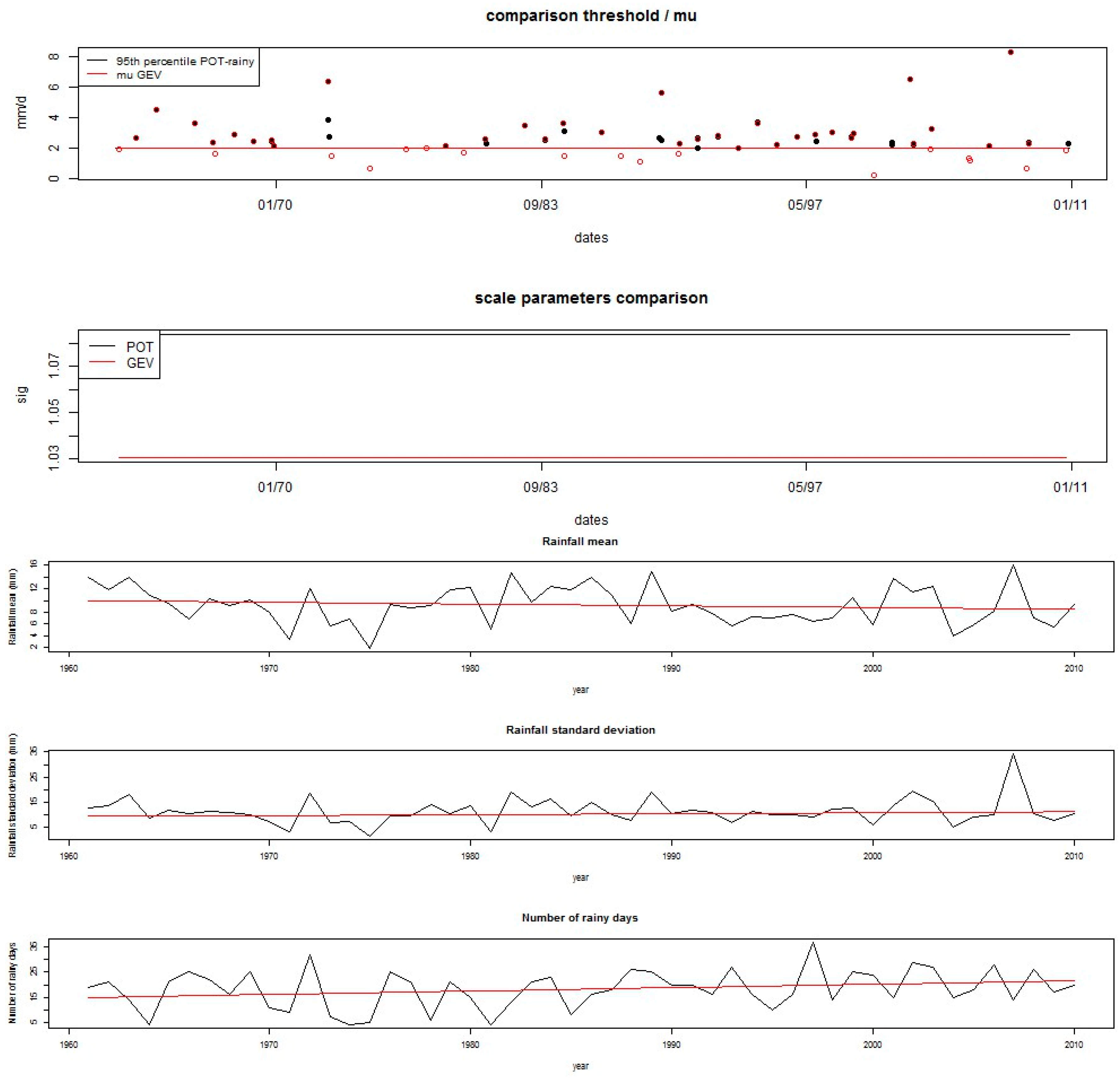
This gauge shows a negative (positive) trend for variance using the BM (POT), leading to different results for Z20 when extrapolating these trends. There is also a positive trend in the number of rainy days. However, the variance with the two methods is different because all-days were used for the BM, but rainy-days-only for the POT. This is another drawback of the BM approach: mixing rainy and non-rainy days mixes two different processes, so that the variance mixes them, as well. Figure 10 shows the comparison between the two approaches using this gauge “mfr” in autumn in the two top panels and the evolution of the mean, standard deviation and number of rainy days in the three bottom panels (seasonal values in black, linear trends in red). This highlights the importance of considering rainy-days-only because, when all days are considered, a positive trend in variance of the rain of rainy days and in the number of rainy days can result in a negative trend in variance.
The gauge that is the exception in spring is “reu” with Z20-POT=51.58 (36.46; 59.10) outside the CI of Z20-GEV=44.80 (33.64; 51.11). It shows a positive trend for variance with both methods, with a more positive trend in the number of rainy days producing a higher Z20 when using the POT technique.
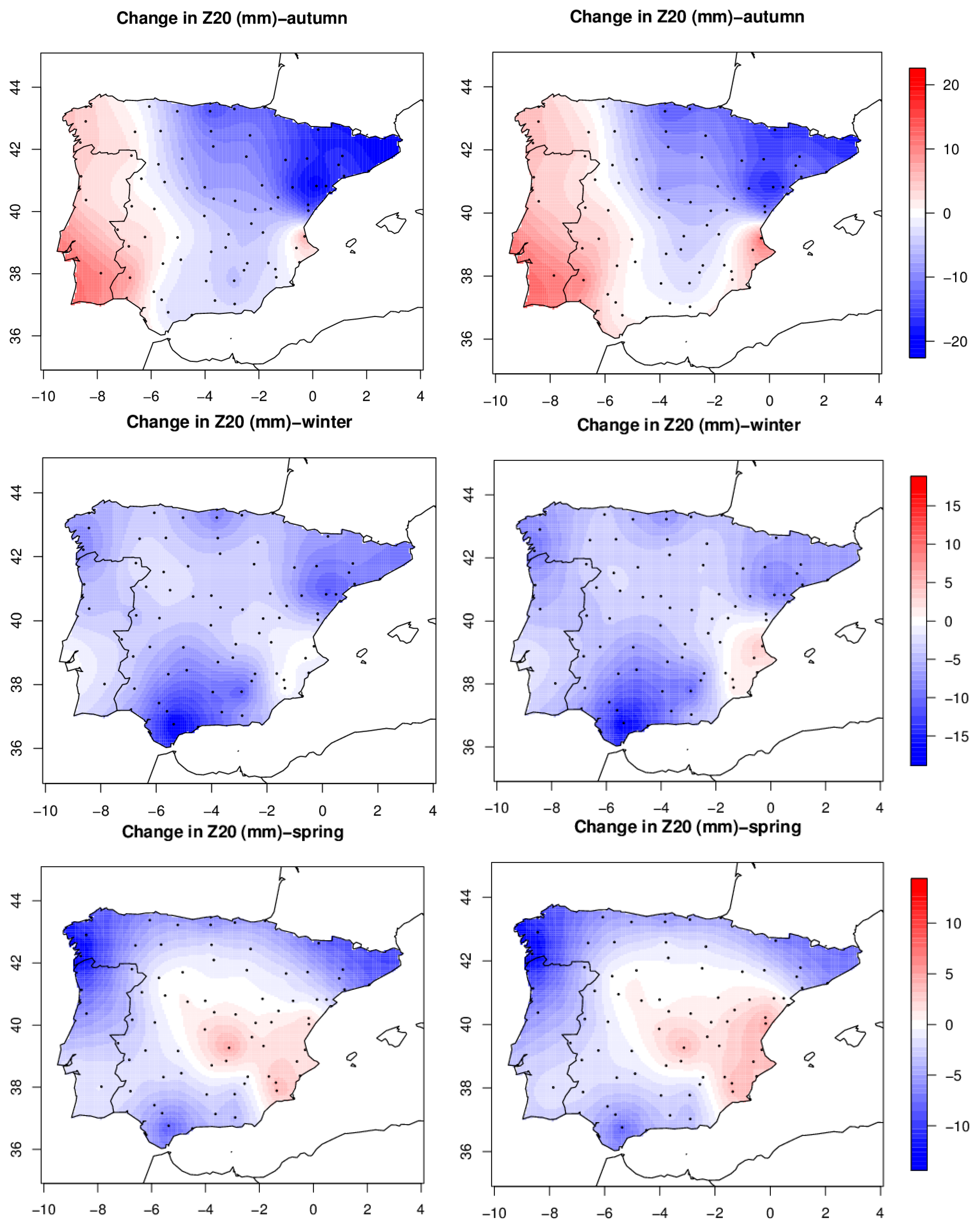
4.4. Changes in Future 20-Year RLs
Although extrapolating recent trends may not be the best approach to computing future RLs, the comparison here was aimed at analyzing the differences induced by changes similar to those already experienced. For both techniques, BM and POT, the spatial distribution of the differences between the 20-year RLs obtained for 2020 using the latter method (stationarity test) and those corresponding to the present day are shown in Figure 11. The changes for the BM are on the left, and those for the POT on the right, with blue (red) meaning decreasing (increasing) values of the 20-year RLs for 2020. The scale used is the same for both approaches. For the three seasons considered, the two approaches usually give similar results, although there are some remarks that need to be made. In autumn, there is an increase in the western IP and a decrease in the east, although there is also an increase in the southeast. The increase in the northeast with the BM (left) is greater than with the POT. In winter, most of the IP presents a decrease in the 20-year RLs for 2020, with only a small area in the southeast having increasing RLs, this being more notable with the POT approach.
5. Discussion
The estimation of the 20-year RLs for the present day with both the BM and the POT approaches led to similar results regardless of whether rainy-days-only or all-days (rainy and non-rainy) datasets were used. There were only a few gauges showing non-overlapping CIs (one for autumn and winter and three for winter), with the RL obtained from the POT approach being greater than that corresponding to the BM. It is important to note that, because of the large number of zeros, the asymptotic assumption in the case of the BM is weakened, i.e., the maximum in the rainfall time series is not the maximum of 90 values (which is of course already quite far from infinity), but of far fewer.
The study of the 20-year RLs for a near-future time obtained through the extrapolation of the trends in the parameters of the extreme value distribution led to similar results for a great part of the gauges using both the BM and the POT approaches, although there were some exceptions. These were mainly related to the decrease of extreme rainfall at the end of the study period. The decrease in location was greater than that in the threshold due to the lower maxima during the last part of the time series. Even if one considers the maxima obtained with the BM approach that are lower than the mobile threshold (red circles in the upper panel of Figure 7), most of them occur at the end of the observation period and also correspond to years that have no maximum precipitation value with the POT approach (black dots in the same figure). This leads to a lower 20-year RL value in 2020 using GEV than using POT when extrapolating the parameters of the extreme value distribution.
The results of the study of the changes between the present day and future 20-year RLs by using the stationarity test were, in general, similar for the BM and POT. They pointed to an important consequence: autumn, instead of winter, would be the season with most extreme rainfall in the western IP due to the sharp increase in the RLs in the future. This is coherent with previous results [9,10] indicating a significant positive trend for extreme rainfall over the western half of the IP and with the findings of a regional study [12] of an area in the southwestern IP, which showed the same behavior. An increase in the frequency of extreme precipitation in autumn for the same area of the IP has been described as being due to increased northwesterly flows [25]. However, most of these changes are not significant because, for most of the gauges, the CIs overlap. This is important because the estimation of RLs is highly uncertain, especially in the context of climate change. In the comparison of the two approaches used to compute the RLs, the stationarity test led to more robust results than using trends in the parameters of the extreme value distribution. The disadvantages of the latter were its reduced sample size, sensitivity to the threshold selection and the fact that there were negative trends in extreme rainfall events at the end of the study period when using the BM. These problems are related to the conclusions drawn in a previous work [12].
The present work has estimated future RLs by extrapolating the observed trends. This does not allow the different signals involved—climate change and inter-annual variability—to be separated. In order to better understand the impact of climate change on extreme rainfall over the IP, complementary analyses with the aid of climate simulations might be necessary. The generally linear trends identified from observed time series and then extrapolated into the future involve both climate change and inter-annual variability signals present in the period of observation. In this sense, there has been a study of how to discriminate the sources of variation in changes of several precipitation characteristics, including heavy precipitation, for the end of the Twenty-First Century over the Rhine Basin [26]. One of the conclusions was that, except for the summer season, natural variability explains a considerable proportion of the variance of the changes in precipitation and is the dominant factor in the winter season. It is noteworthy that extreme rainfall changes for the Iberian Peninsula are different from those in other regions. For instance, some studies have found evidence of increasing trends in intensity for various European regions, with the Czech Republic being an example [27].
6. Conclusions
We have described an EVT study to estimate non-stationary RLs of extreme rainfall for the present day and the near future over the IP. We used a complete dataset of 76 gauges for the period 1961–2010. Two EVT approaches, BM and POT, were applied to estimate the 20-year RLs for the present day and those expected for 2020.
Two methods were used to compute future rainfall RLs with the POT approach. In the first, trends in the extremes were identified considering all-days rainfall data, taking into account a time-varying threshold based on a linear quantile regression and, when appropriate, a trend in the GPD scale parameter. In the second, the RLs were calculated considering rainy-days-only data, examining the impact of evolutions of the mean and variance and of the number of rainy days. In this second case, a novel adaptation of a stationarity test that had been designed and used for temperature time series was applied to rainfall, finding that it was indeed satisfied for most of the gauges for all three seasons considered. As in [12], this second procedure was found to have fewer disadvantages than the first and could therefore be applied in using the evolution of mean and variance projected by climate models for the estimation of future RLs.
The estimation of the present-day 20-year RLs considering all-days (rainy and non-rainy) and rainy-days-only datasets led to similar results for the two approaches, with only a few gauges giving different RLs with BM and POT, as was described in detail in the previous section. When using the BM, the asymptotic assumption is weakened because, in some areas of the IP, the rainfall time series include very many days with zero rainfall, and the BM is sometimes not a real maximum.
This study has estimated the 20-year RLs expect for 2020, with the main objective having been to compare two EVT methods, BM and POT. There were some exceptions to the generally equivalent behavior, which confirmed that POT is a better method for estimating RLs, with BM being less reliable because fixed blocks lead to the selection of non-extreme values. Furthermore, the study of the changes in the near-future RLs over the IP showed that, for some regions, autumn, not winter, is the season with the heaviest rainfall over recent decades due to the increase in the RLs for the western IP.
Acknowledgments
Thanks are due to the Spanish Weather Agency (Agencia Estatal de Meteorología: www.aemet.es) for providing the daily rainfall time series used in this study. This work was partially supported by the Junta de Extremadura—Consejería de Economía e Infraestructuras (FEDER Funds (IB16063)) and Junta de Extremadura (FEDER Funds (GR15137)).
Author Contributions
F.J. Acero. and J.A. García. designed the database. S. Parey and D.D.-Castelle developed the methods. F.J. Acero analyzed the data in accordance with those methods.
Conflicts of Interest
The authors declare no conflict of interest.
References
- Serrano, A.; García, J.A.; Mateos, V.L.; Cancillo, M.L.; Garrido, J. Monthly modes of variation of precipitation over the Iberian Peninsula. J. Clim. 1999, 12, 2894–2919. [Google Scholar] [CrossRef]
- Llasat, M.C.; Puigcerver, M. Total rainfall and convective rainfall in Catalonia, Spain. Int. J. Climatol. 1997, 17, 1683–1695. [Google Scholar] [CrossRef]
- Trigo, R.M.; DaCamara, D.C. Circulation weather types and their impact on the precipitation regime in Portugal. Int. J. Climatol. 2000, 20, 1559–1581. [Google Scholar] [CrossRef]
- Santos, J.A.; Corte-Real, J.; Leite, S.M. Weather regimes and their connection to the winter rainfall in Portugal. Int. J. Climatol. 2005, 25, 33–50. [Google Scholar] [CrossRef]
- Martín-Vide, J. Spatial distribution of a daily precipitation concentration index in Peninsular Spain. Int. J. Climatol. 2004, 24, 959–971. [Google Scholar] [CrossRef]
- Zhang, X.F.; Alexander, L.; Hegerl, G.C.; Jones, P.; Tank, A.K.; Peterson, T.C.; Trewin, B.; Zwiers, F.W. Indices for monitoring changes in extremes based on daily temperature and precipitation data. WIREs Clim. Chang. 2011, 2, 851–870. [Google Scholar] [CrossRef]
- Hidalgo-Muñoz, J.M.; Argüeso, D.; Gámiz-Fortis, S.R.; Esteban-Parra, M.J.; Castro-Díez, Y. Trends of extreme precipitation and associated synoptic patterns over the southern Iberian Peninsula. J. Hydrol. 2011, 409, 497–511. [Google Scholar] [CrossRef]
- Bartolomeu, S.; Carvalho, M.J.; Marta-Almeida, M.; Melo-Gonçalves, P.; Rocha, A. Recent trends of extreme precipitation indices in the Iberian Peninsula using observations and WRF model results. Phys. Chem. Earth 2016, 94, 10–21. [Google Scholar] [CrossRef]
- García, J.A.; Gallego, M.C.; Serrano, A.; Vaquero, J.M. Trends in block-seasonal extreme rainfall over the Iberian Peninsula in the second half of the twentieth century. J. Clim. 2007, 20, 113–120. [Google Scholar] [CrossRef]
- Acero, F.J.; García, J.A.; Gallego, M.C. Peaks-over-threshold study of trends in extreme rainfall over the Iberian Peninsula. J. Clim. 2011, 24, 1089–1105. [Google Scholar] [CrossRef]
- Beguería, S.; Angulo-Martínez, M.; Vicente-Serrano, S.M.; López-Moreno, J.I.; El-Kenawy, A. Assessing trends in extreme precipitation events intensity and magnitude using non-stationary peaks-over-threshold analysis: A case study in northeast Spain from 1930 to 2006. Int. J. Climatol. 2011, 31, 2102–2114. [Google Scholar] [CrossRef] [Green Version]
- Acero, F.J.; Parey, S.; Hoang, T.T.H.; Dacunha-Castelle, D.; García, J.A.; Gallego, M.C. Non-Stationary future return levels for extreme rainfall over Extremadura (southwestern Iberian Peninsula). Hydrol. Sci. J. 2017, 62, 1394–1411. [Google Scholar] [CrossRef]
- Wang, X.L. Detection of undocumented changepoints: A revision of the two-phase regression model. J. Clim. 2003, 16, 3383–3385. [Google Scholar] [CrossRef]
- Wang, X.L.; Weng, Q.H.; Wu, Y. Penalized maximal t test for detecting undocumented mean change in climate data series. J. Appl. Meteorol. Climatol. 2007, 46, 916–931. [Google Scholar] [CrossRef]
- Coles, S. An Introduction to Statistical Modelling of Extreme Values; Springer: London, UK, 2001. [Google Scholar]
- Leadbetter, M.R.; Weissman, I.; Haan, L.D.; Rootzen, H. On clustering of high values in statistically stationary series. Proc. Int. Meet. Stat. Climatol. 1989, 16, 217–222. [Google Scholar]
- Montanari, A.; Koutsoyiannis, D. Modeling and mitigating natural hazards: Stationarity is immortal! Water Resour. Res. 2014, 50, 9748–9756. [Google Scholar] [CrossRef]
- Serinaldi, F.; Kilsby, C.G. Stationarity is undead: Uncertainty dominates the distribution of extremes. Adv. Water Resour. 2015, 77, 17–36. [Google Scholar] [CrossRef]
- Olsen, R.; Lambert, J.H.; Haimes, Y.Y. Risk of extreme events under nonstationary conditions. Risk Anal. 1998, 18, 497–510. [Google Scholar] [CrossRef]
- Parey, S.; Malek, F.; Laurent, C.; Dacunha-Castelle, D. Trends and climate evolution: Statistical approach for very high temperatures in France. Clim. Chang. 2007, 81, 331–352. [Google Scholar] [CrossRef]
- Salas, J.D.; Obeysekera, J. Revisiting the concepts of return period and risk for nonstationary hydrologic extreme events. J. Hydrol. Eng. 2014, 19, 554–568. [Google Scholar] [CrossRef]
- Rootzén, H.; Katz, R.W. Design life level: Quantifying risk in a changing climate. Water Resour. Res. 2013, 49, 5964–5972. [Google Scholar] [CrossRef]
- Liang, Z.; Hu, Y.; Huang, H.; Wang, J.; Li, B. Study on the estimation of design value under non-stationary environment. South North Water Transf. Water Sci. Technol. 2016, 14, 50–53. [Google Scholar]
- Yan, L.; Xiong, L.; Guo, S.; Xu, C.Y.; Xia, J.; Duc, T. Comparison of four nonstationary hydrologic design methods for changing environment. J. Hydrol. 2017, 551, 132–150. [Google Scholar] [CrossRef]
- Fernández-Montes, S.; Seubert, S.; Rodrigo, F.S.; Rasilla Álvarez, D.F.; Hertig, E.; Esteban, P.; Philipp, A. Circulation types and extreme precipitation days in the Iberian Peninsula in the transition seasons: Spatial links and temporal changes. Atmos. Res. 2014, 138, 41–58. [Google Scholar] [CrossRef]
- Hanel, M.; Buishand, T.A. Assessment of the sources of variation in changes of precipitation characteristics over the Rhine Basin using a linear mixed-effects model. J. Clim. 2016, 28, 6903–6919. [Google Scholar] [CrossRef]
- Svoboda, V.; Hanel, M.; Máca, P.; Kyselý, J. Projected changes of rainfall event characteristics for the Czech Republic. J. Hydrol. Hydromech. 2016, 64, 415–425. [Google Scholar] [CrossRef]
Figure 1.
Spatial distribution of the gauges used. The definition of the codes is given in Table 1.
Figure 1.
Spatial distribution of the gauges used. The definition of the codes is given in Table 1.
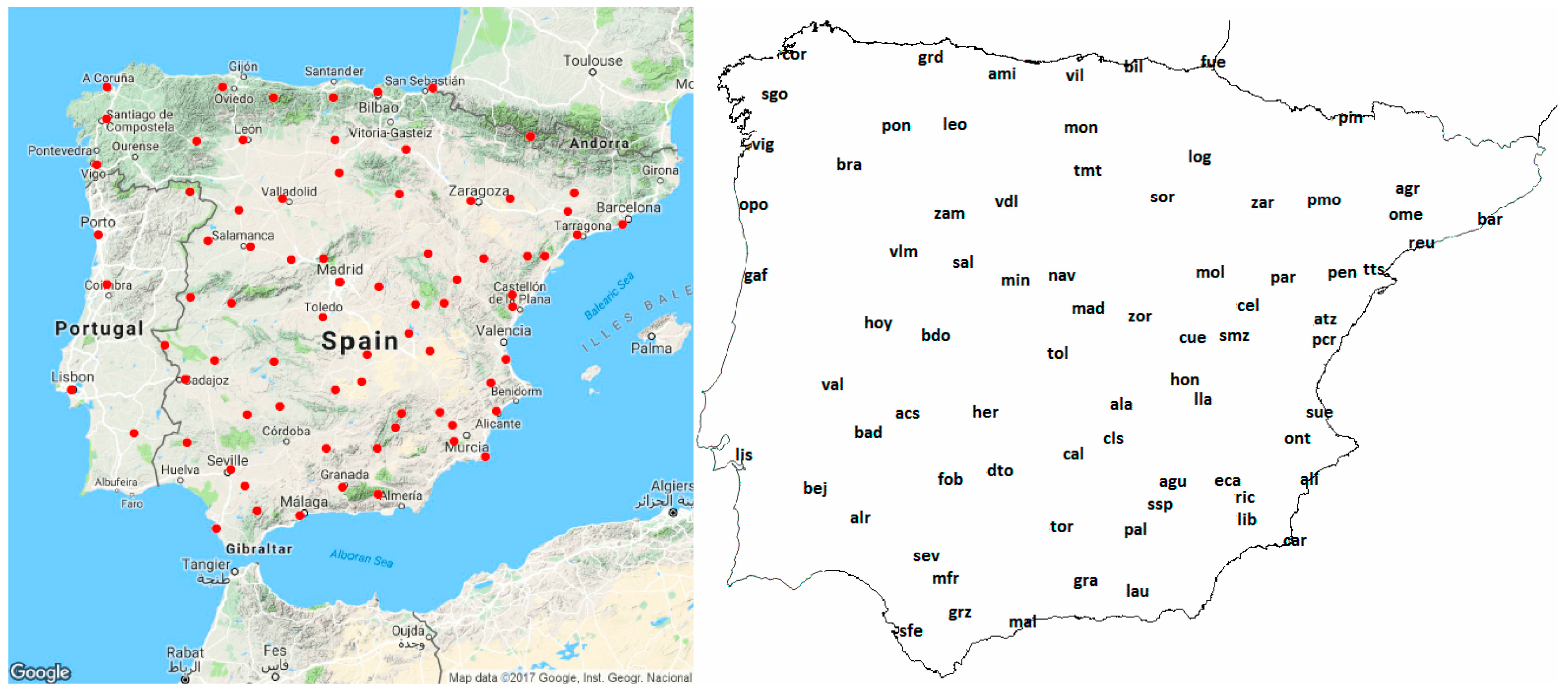
Figure 2.
Spatial distribution of 20-year return levels (RLs) estimated from the all-days data obtained for the peaks-over-threshold (POT) according to whether they do or do not lie within the CI of the 20-year RLs obtained for the block maxima (BM).
Figure 2.
Spatial distribution of 20-year return levels (RLs) estimated from the all-days data obtained for the peaks-over-threshold (POT) according to whether they do or do not lie within the CI of the 20-year RLs obtained for the block maxima (BM).

Figure 3.
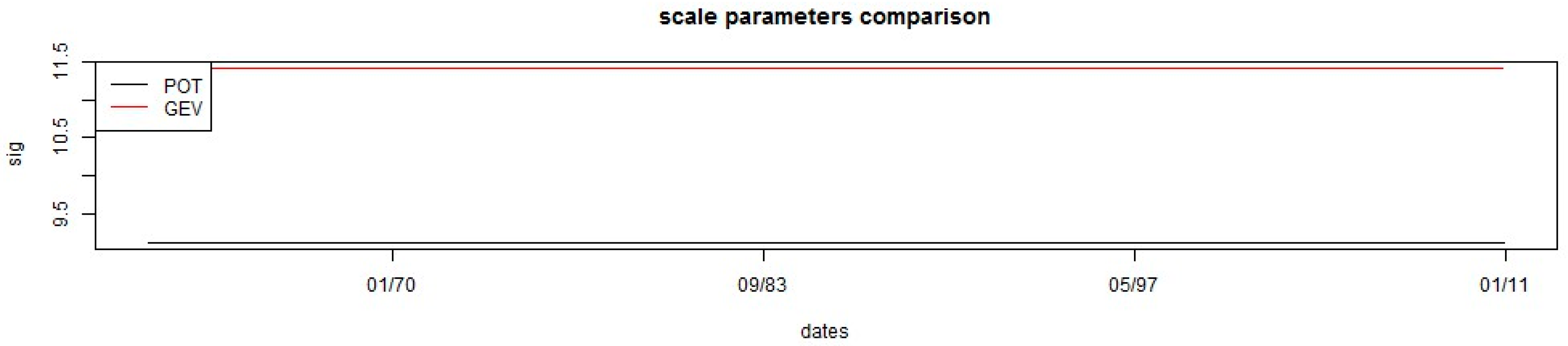
Comparison of GEV/POT for the gauge “vlm” in winter. The top panel shows the comparison between the threshold from the POT and the location parameter from the BM. The symbols show the independent exceedances for the POT (black) and the seasonal maxima for the BM (red). The bottom panel compares the scale parameter between the two methods.
Figure 3.
Comparison of GEV/POT for the gauge “vlm” in winter. The top panel shows the comparison between the threshold from the POT and the location parameter from the BM. The symbols show the independent exceedances for the POT (black) and the seasonal maxima for the BM (red). The bottom panel compares the scale parameter between the two methods.
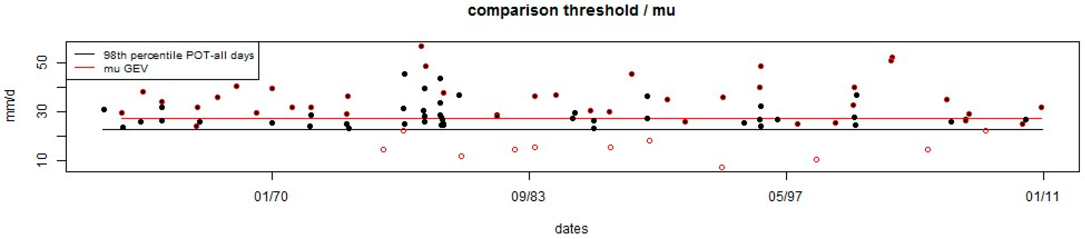

Figure 4.
Similar to Figure 2, but showing the 20-year RLs estimated for the rainy-days-only data.
Figure 4.
Similar to Figure 2, but showing the 20-year RLs estimated for the rainy-days-only data.

Figure 5.
Similar to Figure 3, but showing the comparison GEV/POT for the gauge “pcr” in autumn.
Figure 5.
Similar to Figure 3, but showing the comparison GEV/POT for the gauge “pcr” in autumn.
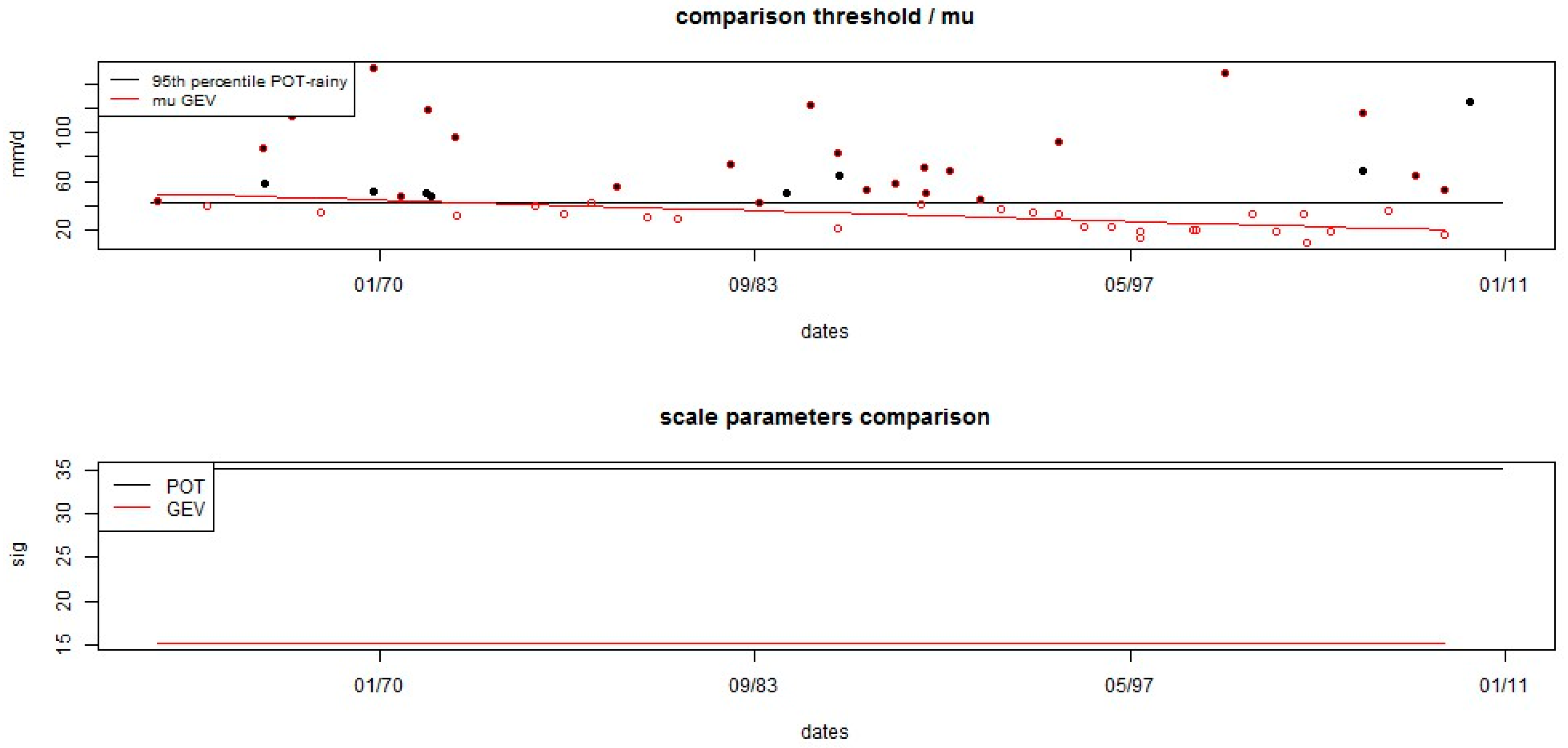
Figure 6.
Spatial distribution of the 20-year RLs for 2020 obtained through extrapolating the location and scale parameters using GEV that lie or do not lie within the CI of the 20-year RLs obtained through extrapolating the scale parameter using the general Pareto distribution (GPD).
Figure 6.
Spatial distribution of the 20-year RLs for 2020 obtained through extrapolating the location and scale parameters using GEV that lie or do not lie within the CI of the 20-year RLs obtained through extrapolating the scale parameter using the general Pareto distribution (GPD).

Figure 7.
Comparison of GEV/POT for the gauge “agr” in autumn.
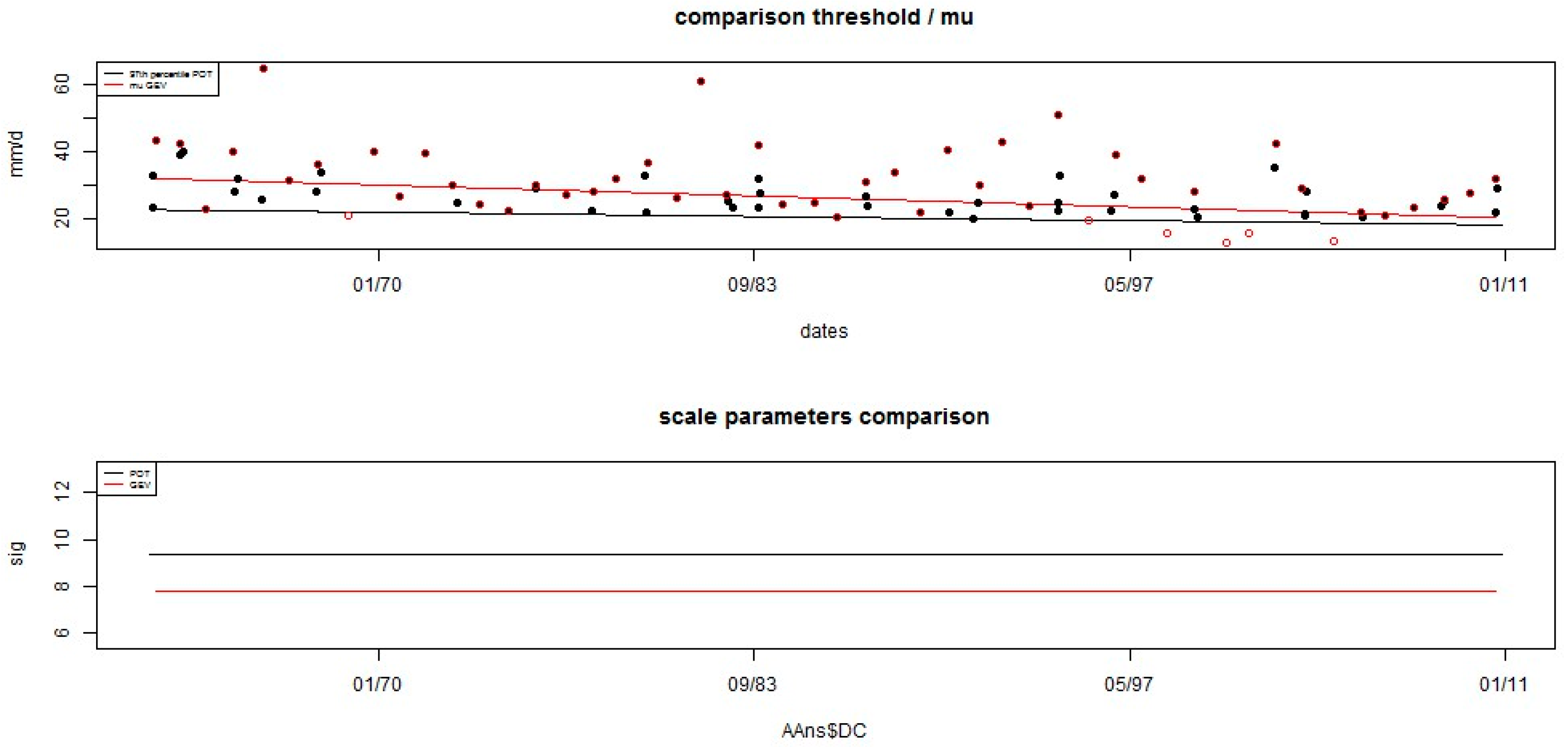
Figure 8.
Comparison of GEV/POT for the gauge “dto” in winter.

Figure 9.
Spatial distribution of the 20-year RLs for 2020 obtained through the stationarity test for the POT that lie or do not lie within the CI of the 20-year RLs for 2020 obtained for the BM.
Figure 9.
Spatial distribution of the 20-year RLs for 2020 obtained through the stationarity test for the POT that lie or do not lie within the CI of the 20-year RLs for 2020 obtained for the BM.

Figure 10.
Comparison of GEV/POT for gauge “mfr” in autumn, but considering Y (two top panels) and the evolution of the mean, standard deviation and number of rainy days (seasonal values in black, linear trends in red) in the three bottom panels.
Figure 10.
Comparison of GEV/POT for gauge “mfr” in autumn, but considering Y (two top panels) and the evolution of the mean, standard deviation and number of rainy days (seasonal values in black, linear trends in red) in the three bottom panels.

Figure 11.
Spatial distribution of the differences between the present and the future for the 20-year RLs (mm) for each season considered, using BM (left) and POT (right).
Figure 11.
Spatial distribution of the differences between the present and the future for the 20-year RLs (mm) for each season considered, using BM (left) and POT (right).

Table 1.
Codes used on the map: names, geographic coordinates, and altitudes of the observatories.
| Code | Name | Latitude (°-′-″) | Longitude (°-′-″) | Altitude (m) |
|---|---|---|---|---|
| acs | Alcuescar | 39-10-50N | 6-13-43W | 488 |
| agr | Agramunt | 41-47-16N | 1-05-54E | 349 |
| agu | Arguellite | 38-20-10N | 2-25-58W | 980 |
| ala | Alameda de Cervera | 39-16-00N | 3-07-38W | 646 |
| ali | Alicante | 38-22-00N | 0-29-40W | 82 |
| alr | Almonaster la Real | 37-52-18N | 6-47-13W | 610 |
| ami | Amieva (Retaño) | 43-13-28N | 5-01-51W | 730 |
| atz | Atzeneta del Maestrat | 40-13-00N | 0-10-17W | 400 |
| bad | Badajoz (Talavera la Real) | 38-53-00N | 6-49-45W | 185 |
| bar | Barcelona | 41-17-49N | 2-04-39E | 6 |
| bdo | Barrado | 40-05-00N | 5-52-57W | 796 |
| bej | Beja | 38-01-00N | 7-52-00W | 246 |
| bil | Bilbao | 43-18-00N | 2-54-36W | 39 |
| bra | Braganza | 41-48-00N | 6-44-00W | 690 |
| cal | Calzada de Calatrava | 38-42-15N | 3-46-17W | 645 |
| car | Cartagena | 37-38-15N | 0-43-02W | 1 |
| cel | Cella | 40-27-20N | 1-17-27W | 1023 |
| cls | San Carlos del Valle | 38-50-40N | 3-14-02W | 753 |
| cor | A Coruña | 43-22-02N | 8-25-10W | 58 |
| cue | Cuenca | 40-04-00N | 2-08-24W | 956 |
| dto | Dos Torres | 38-27-00N | 4-53-57W | 600 |
| eca | Embalse de Camarillas | 38-20-40N | 1-38-56W | 397 |
| fob | Fuenteobejuna | 38-19-30N | 5-33-47W | 571 |
| fue | Fuenterrabía | 43-21-24N | 1-47-25W | 8 |
| gaf | Gafanha da Nazare | 40-37-05N | 8-42-21W | 8 |
| gra | Granada | 37-08-13N | 3-37-53W | 687 |
| grd | Grado | 43-22-39N | 6-04-10W | 60 |
| grz | Grazalema | 36-45-30N | 5-22-07W | 823 |
| her | Herrera del Duque | 39-09-57N | 5-01-09W | 465 |
| hon | Honrubia | 39-36-45N | 2-16-48W | 820 |
| hoy | Hoyos | 40-10-15N | 6-43-17W | 510 |
| lau | Laujar Monterrey | 37-01-35N | 2-53-57W | 1280 |
| leo | León | 42-35-24N | 5-39-00W | 916 |
| lib | Librilla | 37-53-11N | 1-21-22W | 168 |
| lis | Lisboa | 38-43-00N | 9-09-00W | 77 |
| lla | Villagarcia del Llano | 39-19-30N | 1-50-57W | 740 |
| log | Logroño | 42-27-06N | 2-19-51W | 352 |
| mad | Madrid (Retiro) | 40-24-40N | 3-40-41W | 667 |
| mal | Málaga | 36-40-00N | 4-29-17W | 7 |
| mfr | Morón de la Frontera | 37-09-49N | 5-36-43W | 87 |
| min | Mingorria | 40-45-05N | 4-40-02W | 1032 |
| mol | Molina de Aragón | 40-50-40N | 1-53-07W | 1063 |
| mon | Montorio | 42-35-00N | 3-46-42W | 944 |
| nav | Navacerrada | 40-46-50N | 4-00-37W | 1890 |
| ome | Els Omellons | 41-30-06N | 0-57-36E | 386 |
| ont | Ontinyent | 38-49-40N | 0-36-27W | 350 |
| opo | Oporto | 41-08-00N | 8-36-00W | 93 |
| pal | Pozo Alcón (El Hornico) | 37-46-30N | 2-55-07W | 1020 |
| par | Palomar de Arroyos | 40-46-44N | 0-45-04W | 1206 |
| pen | Embalse de Pena | 40-49-17N | 0-08-08E | 620 |
| pcr | Pantano Maria Cristina | 40-01-40N | 0-09-47W | 130 |
| pin | Presa de Pineta | 42-38-08N | 0-12-03E | 1150 |
| pmo | Paracuello de Monegros | 41-42-17N | 0-12-41W | 356 |
| pon | Ponferrada | 42-33-50N | 6-36-00W | 534 |
| reu | Reus | 41-08-45N | 1-09-36E | 73 |
| ric | Ricote (La Calera) | 38-08-46N | 1-22-58W | 480 |
| sal | Salamanca (Matacán) | 40-56-50N | 5-29-41W | 790 |
| sev | Sevilla | 37-25-26N | 5-54-13W | 26 |
| ssp | Santiago de la Espada | 38-06-44N | 2-33-10W | 1340 |
| sfe | San Fernando | 36-28-00N | 6-12-00W | 97 |
| sgo | Santiago de Compostela | 42-54-00N | 8-26-00W | 364 |
| smz | Salinas del Manzano | 40-05-30N | 1-33-17W | 1155 |
| sor | Soria | 41-46-00N | 2-28-00W | 1082 |
| sue | Sueca | 39-12-00N | 0-18-17W | 7 |
| tmt | Torrecilla del Monte | 42-05-40N | 3-41-37W | 949 |
| tol | Toledo (Lorenzana) | 39-51-34N | 4-01-32W | 540 |
| tor | Torredonjimeno | 37-45-54N | 3-57-25W | 591 |
| tts | Tortosa | 40-49-14N | 0-29-29E | 48 |
| val | Valencia de Alcántara | 39-24-58N | 7-14-52W | 460 |
| vdl | Valladolid | 41-38-40N | 4-46-27W | 846 |
| vig | Vigo | 42-13-25N | 8-37-55W | 255 |
| vil | Villacarriedo | 43-13-37N | 3-48-38W | 212 |
| vlm | Villarmuerto | 41-03-20N | 6-21-47W | 767 |
| zam | Zamora | 41-29-56N | 5-45-20W | 656 |
| zar | Zaragoza | 41-39-43N | 1-00-29W | 247 |
| zor | Salto de Zorita | 40-20-35N | 2-52-57W | 642 |
Table 2.
Degree of the parameters for GEV (location and scale) and POT (scale) for autumn. Zero means no trend and 1 linear trend.
Table 2.
Degree of the parameters for GEV (location and scale) and POT (scale) for autumn. Zero means no trend and 1 linear trend.
| Code | agr | alr | bra | cue | log | mad | sgo | atz | sue | vil |
|---|---|---|---|---|---|---|---|---|---|---|
| Location-GEV | 1 | 0 | 0 | 0 | 0 | 0 | 0 | 0 | 0 | 1 |
| Scale-GEV | 0 | 0 | 0 | 1 | 0 | 1 | 0 | 0 | 1 | 0 |
| Scale-POT | 0 | 1 | 0 | 0 | 0 | 0 | 1 | 1 | 0 | 1 |
| Red. open (not overlapping and POT RL > GEV RL) | Red. filled (not overlapping and POT RL < GEV RL) | |||||||||
Table 3.
Degree of the parameters for GEV (location and scale) and POT (scale) for winter. Zero means no trend and 1 linear trend.
Table 3.
Degree of the parameters for GEV (location and scale) and POT (scale) for winter. Zero means no trend and 1 linear trend.
| Code | cal | dto | eca | lib | log | val | alr | bad | reu | vig | vil |
|---|---|---|---|---|---|---|---|---|---|---|---|
| Location-GEV | 1 | 1 | 0 | 1 | 0 | 0 | 0 | 0 | 0 | 0 | 0 |
| Scale-GEV | 0 | 0 | 0 | 0 | 0 | 0 | 1 | 0 | 0 | 0 | 0 |
| Scale-POT | 0 | 0 | 0 | 1 | 0 | 1 | 0 | 0 | 1 | 1 | 0 |
| Red. open (not overlapping and POT RL > GEV RL) | Red. filled (not overlapping and POT RL < GEV RL) | ||||||||||
Table 4.
Degree of the parameters for GEV (location and scale) and POT (scale) for spring. Zero means no trend and 1 linear trend.
Table 4.
Degree of the parameters for GEV (location and scale) and POT (scale) for spring. Zero means no trend and 1 linear trend.
| Code | agu | cue | mon | vdl | nav |
|---|---|---|---|---|---|
| Location-GEV | 0 | 0 | 0 | 0 | 0 |
| Scale-GEV | 1 | 1 | 0 | 0 | 0 |
| Scale-POT | 0 | 0 | 1 | 1 | 1 |
| Red. open (not overlapping and POT RL > GEV RL) | Red. filled (not overlapping and POT RL < GEV RL) | ||||
Table 5.
Percentage of the stations that completely satisfied the stationarity of the extremes of the residuals for the three seasons considered, using the two methods.
Table 5.
Percentage of the stations that completely satisfied the stationarity of the extremes of the residuals for the three seasons considered, using the two methods.
| GEV | POT | |
|---|---|---|
| Autumn | 87% | 95% |
| Winter | 78% | 92% |
| Spring | 87% | 95% |
© 2018 by the authors. Licensee MDPI, Basel, Switzerland. This article is an open access article distributed under the terms and conditions of the Creative Commons Attribution (CC BY) license (http://creativecommons.org/licenses/by/4.0/).
Share and Cite
MDPI and ACS Style
Acero, F.J.; Parey, S.; García, J.A.; Dacunha-Castelle, D. Return Level Estimation of Extreme Rainfall over the Iberian Peninsula: Comparison of Methods. Water 2018, 10, 179. https://doi.org/10.3390/w10020179
AMA Style
Acero FJ, Parey S, García JA, Dacunha-Castelle D. Return Level Estimation of Extreme Rainfall over the Iberian Peninsula: Comparison of Methods. Water. 2018; 10(2):179. https://doi.org/10.3390/w10020179
Chicago/Turabian StyleAcero, Francisco Javier, Sylvie Parey, José Agustín García, and Didier Dacunha-Castelle. 2018. "Return Level Estimation of Extreme Rainfall over the Iberian Peninsula: Comparison of Methods" Water 10, no. 2: 179. https://doi.org/10.3390/w10020179
Note that from the first issue of 2016, this journal uses article numbers instead of page numbers. See further details here.