Climate Change Demands Adaptive Management of Urban Lakes: Model-Based Assessment of Management Scenarios for Lake Tegel (Berlin, Germany)

 ,
,
Abstract
: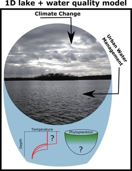
1. Introduction
2. Materials and Methods
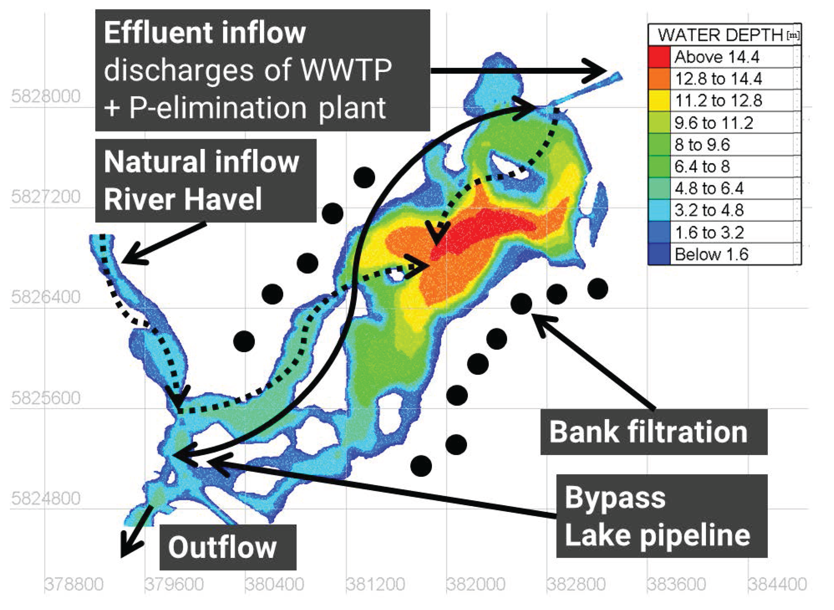
2.1. Study Site
2.2. Model Description and Input Data
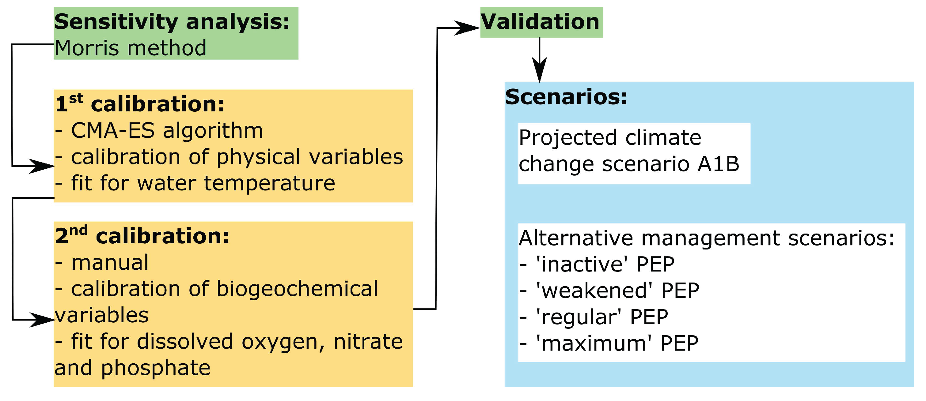
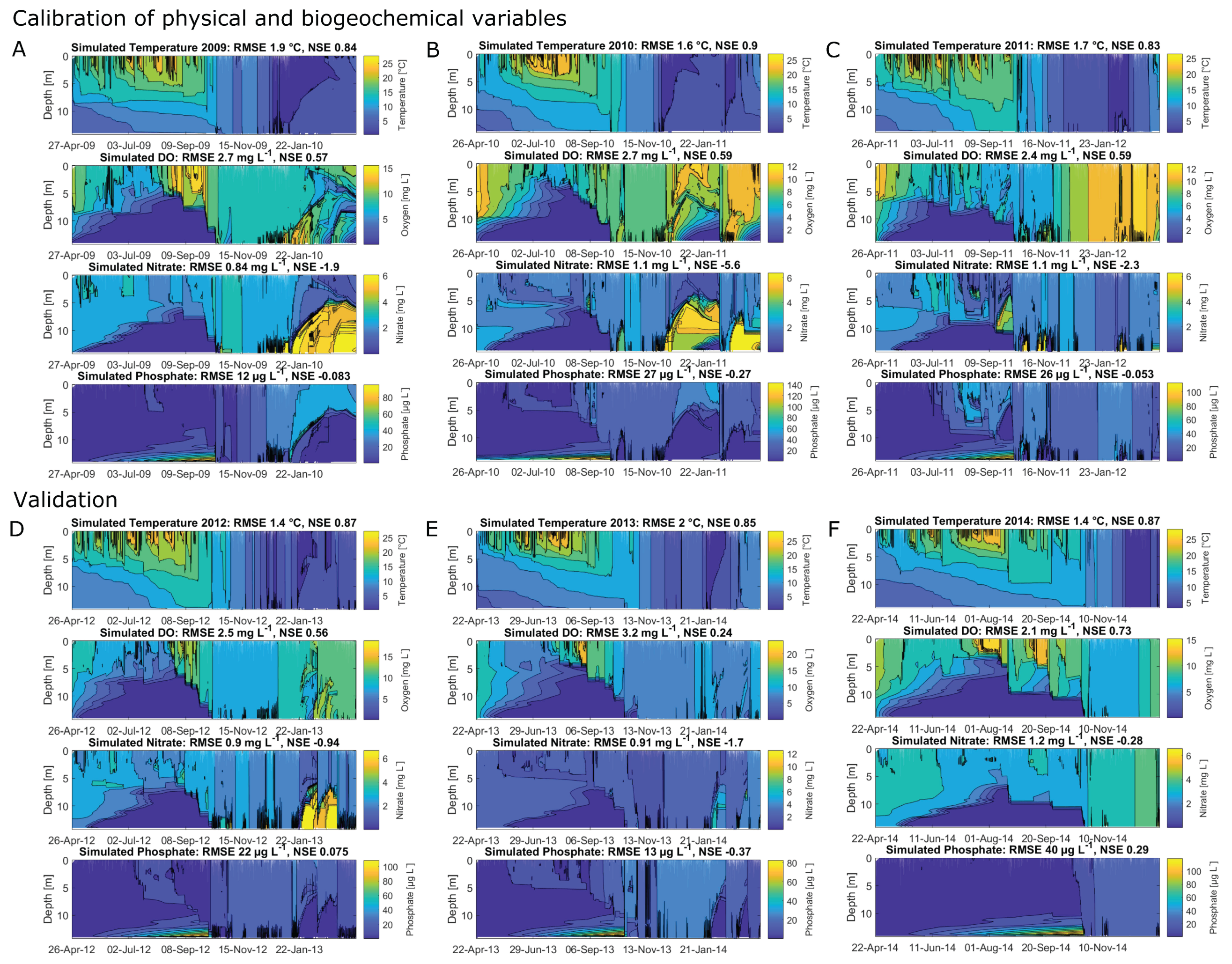
2.3. Calibration and Validation
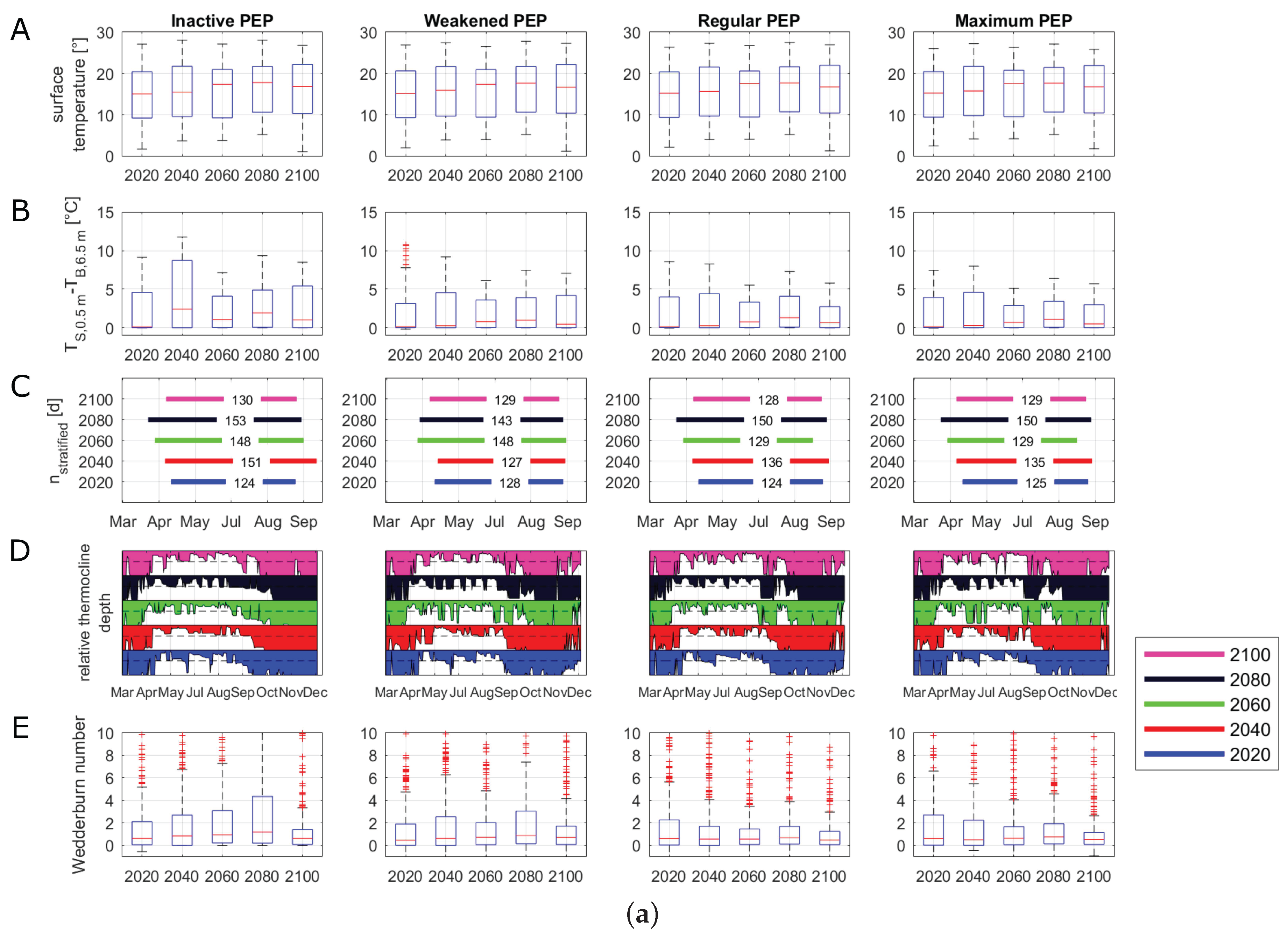
2.4. Scenarios
- Inactive: discharge is set to a constant value of 0 , and the elimination plant becomes deactivated: Q = 0 ± .
- Weakened: for each year, we used the mean daily discharges from the period 1996–2001, when the lake pipeline, supporting the elimination plant, was deactivated: Q = 1.47 ± .
- Regular: for each year, we used the mean daily discharges from our field data for 2008–2014: Q = 2.53 ± .
- Maximum: for each year, we set the daily discharge to a constant value of : Q = 3.5 ± .
- The surface water temperatures ().
- The duration of stratification between onset and breakdown; we determined the onset and breakdown of stratification as the day on which the temperature difference was over or under 1 and the mean temperature difference of the next 14 days was also over or under 1 .
- The thermocline depths (using the LakeAnalyzer software); the thermocline depths were normalized between 0 and 1.
- The dimensionless Wedderburn number [65], where h is the depth of the mixed layer (), is the water friction velocity due to wind stress (), is the previously explained reduced gravitational acceleration, and L is the fetch length (); W is an indicator for the breakdown of lake stratification [66] (using the LakeAnalyzer software).
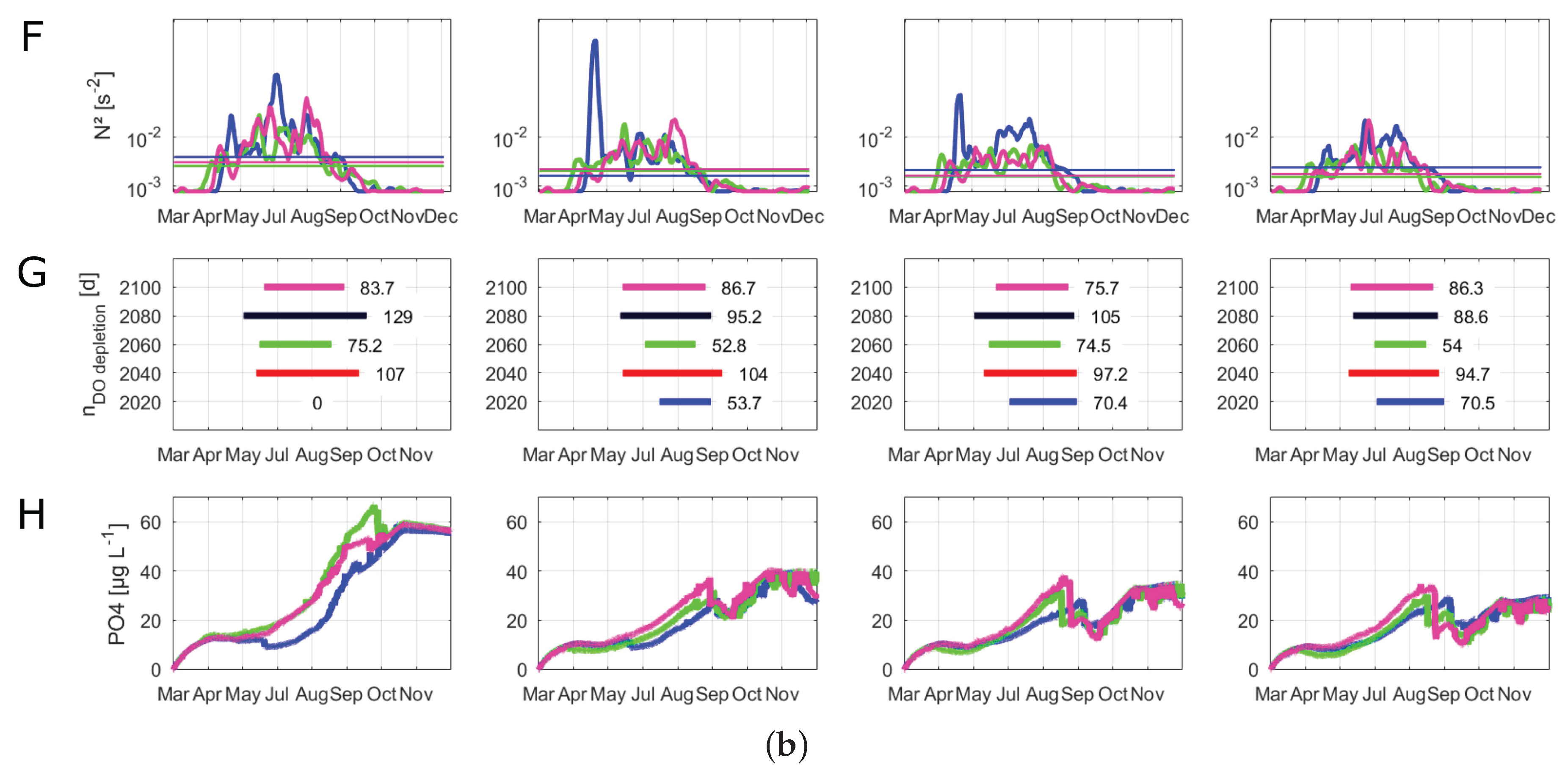
- The buoyancy frequency () as an indicator for phytoplankton habitat conditions (using the LakeAnalyzer software).
- The duration of critical bottom oxygen concentrations under 2 mg L; we determined the start and end date of oxygen depletion as the day on which the mean oxygen concentration at depths from 10 to 15 was over or under 2 mg L and the mean oxygen concentration of the next 14 days was also over or under 2 mg L.
3. Results
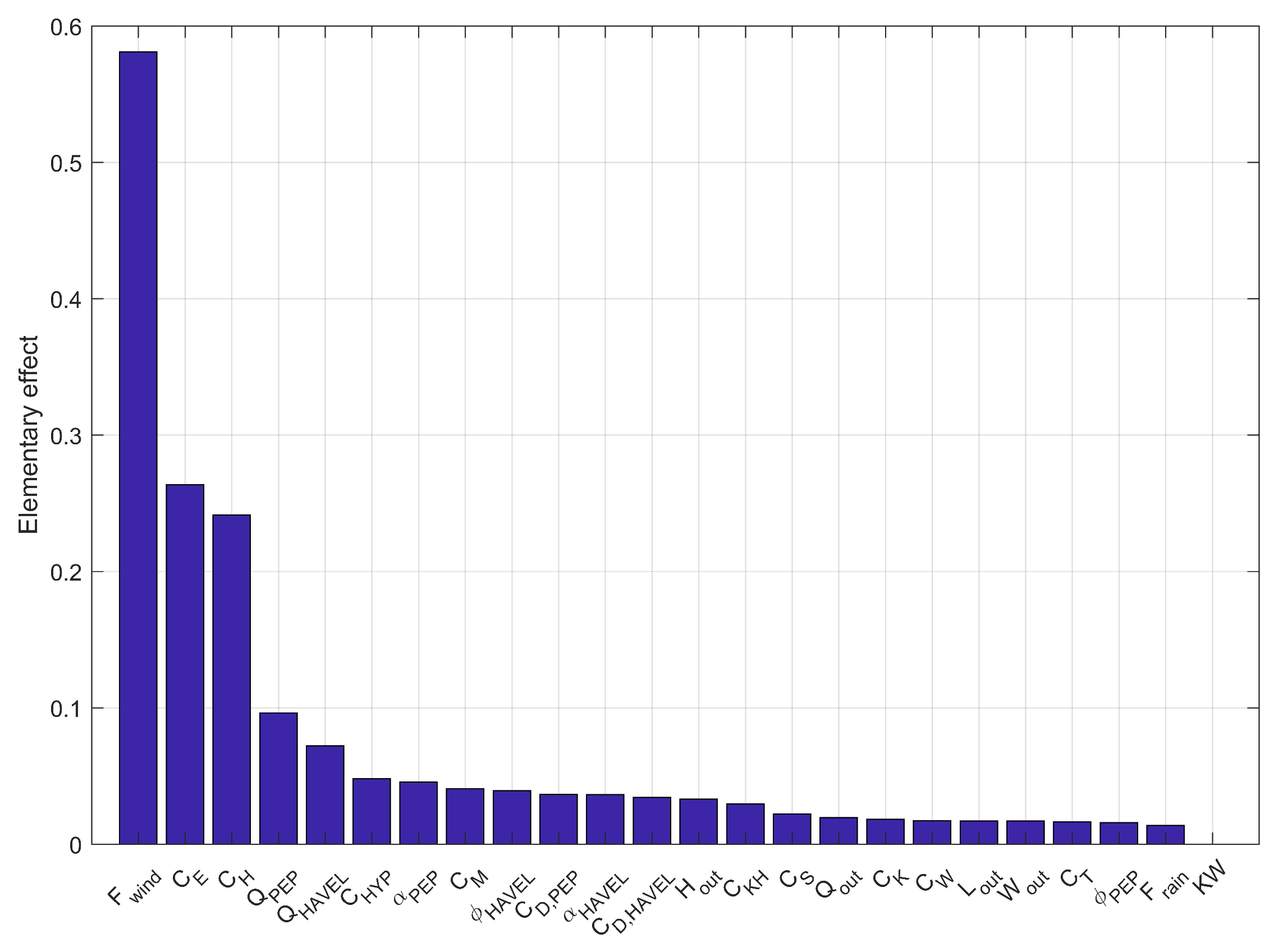
3.1. Sensitivity Analysis, Calibration and Validation
3.2. Climate Change and Alternative Management Scenarios
4. Discussion
4.1. Model Application
4.2. Assessment of Scenarios
4.3. Implications for the Lake Water Management
5. Conclusions
Acknowledgments
Author Contributions
Conflicts of Interest
Abbreviations
| AED2 | Aquatic Ecodynamics Model Library |
| CMA-ES | Covariance Matrix Adaption Evolution Strategy |
| DOC | Dissolved organic carbon |
| EE | Elementary effect |
| GLM | General Lake Model |
| NRMSE | Normalized root-mean-square error |
| NSE | Nash–Sutcliffe coefficient of efficiency |
| PEP | Phosphorus elimination plant |
| POC | Particulate organic carbon |
| RMSE | Root-mean-square error |
| WETTREG | Wetterlagen-basierte Regionalisierungsmethode (regionalization method) |
| WWTP | Wastewater treatment plant |
Appendix A


| Year | Surface | Bottom | ||||||
|---|---|---|---|---|---|---|---|---|
| T | N | P | T | N | P | |||
| 2008 | 0.17 | 2.1 | 0.17 | 6.6 | 0.51 | 0.48 | 0.54 | 10 |
| 2009 | 0.41 | 2.7 | 0.19 | 2.6 | 0.89 | 0.94 | 0.45 | 8.6 |
| 2010 | 0.74 | 2.1 | 0.09 | 5.3 | 0.24 | 0.72 | 0.4 | 21 |
| 2011 | 0.73 | 1.9 | 0.22 | 6.1 | 0.4 | 0.72 | 0.41 | 17 |
| 2012 | 0.31 | 2.6 | 0.12 | 2.3 | 0.32 | 0.53 | 0.40 | 11 |
| 2013 | 0.53 | 3.1 | 0.18 | 3.1 | 0.2 | 1.0 | 0.52 | 5.7 |
| 2014 | 0.36 | 2.7 | 0.51 | 2.0 | 0.2 | 0.51 | 0.36 | 29 |
References
- Sala, O.E.; Chapin, F.S.; Armesto, J.J.; Berlow, E.; Bloomfield, J.; Dirzo, R.; Huber-Sanwald, E.; Huenneke, L.F.; Jackson, R.B.; Kinzig, A.; et al. Global Biodiversity Scenarios for the Year 2100. Science 2000, 287, 1770–1774. [Google Scholar] [CrossRef] [PubMed]
- Walther, G.R.; Post, E.; Convey, P.; Menzel, A.; Parmesan, C.; Beebee, T.J.C.; Fromentin, J.M.; Hoegh-Guldberg, O.; Bairlein, F. Ecological responses to recent climate change. Nature 2002, 416, 389–395. [Google Scholar] [CrossRef] [PubMed]
- Whitehead, P.G.; Wilby, R.L.; Battarbee, R.W.; Kernan, M.; Wade, A.J. A review of the potential impacts of climate change on surface water quality. Hydrol. Sci. J. 2009, 54, 101–123. [Google Scholar] [CrossRef]
- Adrian, R.; O’Reilly, C.M.; Zagarese, H.; Baines, S.B.; Hessen, D.O.; Keller, W.; Livingstone, D.M.; Sommaruga, R.; Straile, D.; Van Donk, E.; et al. Lakes as sentinels of climate change. Limnol. Oceanogr. 2009, 54, 2283–2297. [Google Scholar] [CrossRef] [PubMed] [Green Version]
- Jiménez Cisneros, B.; Oki, T.; Arnell, N.; Benito, G.; Cogley, J.; Döll, P.; Jiang, T.; Mwakalila, S. Climate Change 2014: Impacts, Adaptation, and Vulnerability. Part A: Global and Sectoral Aspects. Contribution of Working Group II to the Fifth Assessment Report of the Intergovernmental Panel on Climate Change; Cambridge University Press: Cambridge, UK, 2014; Chapter Freshwater Resources; pp. 229–269. [Google Scholar]
- Landkildehus, F.; Søndergaard, M.; Beklioglu, M.; Adrian, R.; Angeler, D.G.; Hejzlar, J.; Papastergiadou, E.; Zingel, P.; Çakiroǧlu, A.I.; Scharfenberger, U.; et al. Climate change effects on shallow lakes: Design and preliminary results of a cross-European climate gradient mesocosm experiment. Est. J. Ecol. 2014, 63, 71. [Google Scholar] [CrossRef]
- Grimm, N.B.; Faeth, S.H.; Golubiewski, N.E.; Redman, C.L.; Wu, J.; Bai, X.; Briggs, J.M. Global Change and the Ecology of Cities. Science 2008, 319, 756–760. [Google Scholar] [CrossRef] [PubMed]
- Abdel-Fattah, S.; Krantzberg, G. Commentary: Climate change adaptive management in the Great Lakes. J. Great Lakes Res. 2014, 40, 578–580. [Google Scholar] [CrossRef]
- Graham, N.E.; Georgakakos, K.P. Toward Understanding the Value of Climate Information for Multiobjective Reservoir Management under Present and Future Climate and Demand Scenarios. J. Appl. Meteor. Climatol. 2009, 49, 557–573. [Google Scholar] [CrossRef]
- Yasarer, L.M.W.; Sturm, B.S.M. Potential impacts of climate change on reservoir services and management approaches. Lake Reserv. Manag. 2016, 32, 13–26. [Google Scholar] [CrossRef]
- Jeppesen, E.; Meerhoff, M.; Davidson, T.A.; Trolle, D.; Søndergaard, M.; Lauridsen, T.L.; Beklioglu, M.; Brucet, S.; Volta, P.; González-Bergonzoni, I.; et al. Climate change impacts on lakes: An integrated ecological perspective based on a multi-faceted approach, with special focus on shallow lakes. J. Limnol. 2014, 73. [Google Scholar] [CrossRef] [Green Version]
- O’Reilly, C.M.; Sharma, S.; Gray, D.K.; Hampton, S.E.; Read, J.S.; Rowley, R.J.; Schneider, P.; Lenters, J.D.; McIntyre, P.B.; Kraemer, B.M.; et al. Rapid and highly variable warming of lake surface waters around the globe. Geophys. Res. Lett. 2015, 42, 2015GL066235. [Google Scholar] [CrossRef]
- Havens, K.E.; Paerl, H.W. Climate Change at a Crossroad for Control of Harmful Algal Blooms. Environ. Sci. Technol. 2015, 49, 12605–12606. [Google Scholar] [CrossRef] [PubMed]
- Paerl, H.W. Mitigating Harmful Cyanobacterial Blooms in a Human- and Climatically-Impacted World. Life 2014, 4, 988–1012. [Google Scholar] [CrossRef] [PubMed]
- Trolle, D.; Elliott, J.A.; Mooij, W.M.; Janse, J.H.; Bolding, K.; Hamilton, D.P.; Jeppesen, E. Advancing projections of phytoplankton responses to climate change through ensemble modelling. Environ. Model. Softw. 2014, 61, 371–379. [Google Scholar] [CrossRef]
- Kirillin, G. Modeling the impact of global warming on water temperature and seasonal mixing regimes in small temperate lakes. Boreal Environ. Res. 2010, 15, 279–293. [Google Scholar]
- Sahoo, G.B.; Forrest, A.L.; Schladow, S.G.; Reuter, J.E.; Coats, R.; Dettinger, M. Climate change impacts on lake thermal dynamics and ecosystem vulnerabilities. Limnol. Oceanogr. 2016, 61, 496–507. [Google Scholar] [CrossRef]
- Magee, M.R.; Wu, C.H. Response of water temperatures and stratification to changing climate in three lakes with different morphometry. Hydrol. Earth Syst. Sci. 2017, 21, 6253–6274. [Google Scholar] [CrossRef]
- Zhang, W.; Xu, Q.; Wang, X.; Hu, X.; Wang, C.; Pang, Y.; Hu, Y.; Zhao, Y.; Zhao, X. Spatiotemporal Distribution of Eutrophication in Lake Tai as Affected by Wind. Water 2017, 9, 200. [Google Scholar] [CrossRef]
- Rose, K.C.; Winslow, L.A.; Read, J.S.; Hansen, G.J.A. Climate-induced warming of lakes can be either amplified or suppressed by trends in water clarity. Limnol. Oceanogr. 2016, 1, 44–53. [Google Scholar] [CrossRef]
- Snortheim, C.A.; Hanson, P.C.; McMahon, K.D.; Read, J.S.; Carey, C.C.; Dugan, H.A. Meteorological drivers of hypolimnetic anoxia in a eutrophic, north temperate lake. Ecol. Model. 2017, 343, 39–53. [Google Scholar] [CrossRef]
- Read, J.S.; Winslow, L.A.; Hansen, G.J.; Van Den Hoek, J.; Hanson, P.C.; Bruce, L.C.; Markfort, C.D. Simulating 2368 temperate lakes reveals weak coherence in stratification phenology. Ecol. Model. 2014, 291, 142–150. [Google Scholar] [CrossRef]
- Gessner, M.; Hinkelmann, R.; Nützmann, G.; Jekel, M.; Singer, G.; Lewandowski, J.; Nehls, T.; Barjenbruch, M. Urban water interfaces. J. Hydrol. 2014, 514, 226–232. [Google Scholar] [CrossRef]
- Jekel, M.; Ruhl, A.; Meinel, F.; Zietzschmann, F.; Lima, S.; Baur, N.; Wenzel, M.; Gnirß, R.; Sperlich, A.; Dünnbier, U.; et al. Anthropogenic organic micro-pollutants and pathogens in the urban water cycle: Assessment, barriers and risk communication (ASKURIS). Environ. Sci. Eur. 2013, 25, 20. [Google Scholar] [CrossRef] [Green Version]
- Jeppesen, E.; Søndergaard, M.; Liu, Z. Lake Restoration and Management in a Climate Change Perspective: An Introduction. Water 2017, 9, 122. [Google Scholar] [CrossRef]
- Kaushal, S.S.; McDowell, W.H.; Wollheim, W.M.; Johnson, T.A.N.; Mayer, P.M.; Belt, K.T.; Pennino, M.J. Urban Evolution: The Role of Water. Water 2015, 7, 4063–4087. [Google Scholar] [CrossRef]
- Sahoo, G.B.; Schladow, S.G. Impacts of climate change on lakes and reservoirs dynamics and restoration policies. Sustain. Sci. 2008, 3, 189–199. [Google Scholar] [CrossRef]
- Garrote, L. Managing Water Resources to Adapt to Climate Change: Facing Uncertainty and Scarcity in a Changing Context. Water Resour. Manag. 2017, 31, 2951–2963. [Google Scholar] [CrossRef]
- Simonovic, S.P. Bringing Future Climatic Change into Water Resources Management Practice Today. Water Resour. Manag. 2017, 31, 2933–2950. [Google Scholar] [CrossRef]
- Goonetilleke, A.; Vithanage, M. Water Resources Management: Innovation and Challenges in a Changing World. Water 2017, 9, 281. [Google Scholar] [CrossRef]
- Wang, G.; Mang, S.; Cai, H.; Liu, S.; Zhang, Z.; Wang, L.; Innes, J.L. Integrated watershed management: evolution, development and emerging trends. J. For. Res. 2016, 27, 967–994. [Google Scholar] [CrossRef]
- Ludovisi, A.; Gaino, E.; Bellezza, M.; Casadei, S. Impact of climate change on the hydrology of shallow Lake Trasimeno (Umbria, Italy): History, forecasting and management. Aquat. Ecosyst. Health Manag. 2013, 16, 190–197. [Google Scholar] [CrossRef]
- Tzabiras, J.; Vasiliades, L.; Sidiropoulos, P.; Loukas, A.; Mylopoulos, N. Evaluation of Water Resources Management Strategies to Overturn Climate Change Impacts on Lake Karla Watershed. Water Resour. Manag. 2016, 30, 5819–5844. [Google Scholar] [CrossRef]
- Zhang, C.; Lai, S.; Gao, X.; Xu, L. Potential impacts of climate change on water quality in a shallow reservoir in China. Environ. Sci. Pollut. Res. 2015, 22, 14971–14982. [Google Scholar] [CrossRef] [PubMed]
- Germer, S.; Kaiser, K.; Bens, O.; Hüttl, R.F. Water Balance Changes and Responses of Ecosystems and Society in the Berlin-Brandenburg Region—A Review. DIE ERDE J. Geogr. Soc. Berlin 2011, 142, 65–95. [Google Scholar]
- Andrew, J.T.; Sauquet, E. Climate Change Impacts and Water Management Adaptation in Two Mediterranean-Climate Watersheds: Learning from the Durance and Sacramento Rivers. Water 2017, 9, 126. [Google Scholar] [CrossRef]
- Fant, C.; Srinivasan, R.; Boehlert, B.; Rennels, L.; Chapra, S.C.; Strzepek, K.M.; Corona, J.; Allen, A.; Martinich, J. Climate Change Impacts on US Water Quality Using Two Models: HAWQS and US Basins. Water 2017, 9, 118. [Google Scholar] [CrossRef]
- Schauser, I.; Chorus, I. Assessment of internal and external lake restoration measures for two Berlin lakes. Lake Reserv. Manag. 2007, 23, 366–376. [Google Scholar] [CrossRef]
- Hilt, S.; Van de Weyer, K.; Köhler, A.; Chorus, I. Submerged Macrophyte Responses to Reduced Phosphorus Concentrations in Two Peri-Urban Lakes. Restor. Ecol. 2010, 18, 452–461. [Google Scholar] [CrossRef]
- Heinzmann, B.; Chorus, I. Restoration concept for Lake Tegel, a major drinking and bathing water resource in a densely populated area. Environ. Sci. Technol. 1994, 28, 1410–1416. [Google Scholar] [CrossRef] [PubMed]
- Kleeberg, A.; Köhler, A.; Hupfer, M. How effectively does a single or continuous iron supply affect the phosphorus budget of aerated lakes? J. Soils Sediments 2012, 12, 1593–1603. [Google Scholar] [CrossRef]
- Ladwig, R.; Heinrich, L.; Singer, G.; Hupfer, M. Sediment core data reconstruct the management history and usage of a heavily modified urban lake in Berlin, Germany. Environ. Sci. Pollut. Res. 2017, 24, 25166–25178. [Google Scholar] [CrossRef] [PubMed]
- Schauser, I.; Chorus, I. Water and phosphorus mass balance of Lake Tegel and Schlachtensee—A modelling approach. Water Res. 2009, 43, 1788–1800. [Google Scholar] [CrossRef] [PubMed]
- Lindenschmidt, K.E.; Hamblin, P.F. Hypolimnetic aeration in Lake Tegel, Berlin. Water Res. 1997, 31, 1619–1628. [Google Scholar] [CrossRef]
- Schimmelpfennig, S.; Kirillin, G.; Engelhardt, C.; Nützmann, G. Effects of wind-driven circulation on river intrusion in Lake Tegel: Modeling study with projection on transport of pollutants. Environ. Fluid Mech. 2012, 12, 321–339. [Google Scholar] [CrossRef]
- Schimmelpfennig, S.; Kirillin, G.; Engelhardt, C.; Nützmann, G.; Dünnbier, U. Seeking a compromise between pharmaceutical pollution and phosphorus load: Management strategies for Lake Tegel, Berlin. Water Res. 2012, 46, 4153–4163. [Google Scholar] [CrossRef] [PubMed]
- Read, J.S.; Hamilton, D.P.; Jones, I.D.; Muraoka, K.; Winslow, L.A.; Kroiss, R.; Wu, C.H.; Gaiser, E. Derivation of lake mixing and stratification indices from high-resolution lake buoy data. Environ. Model. Softw. 2011, 26, 1325–1336. [Google Scholar] [CrossRef]
- Patterson, J.C.; Hamblin, P.F.; Imberger, J. Classification and dynamic simulation of the vertical density structure of lakes1. Limnol. Oceanogr. 1984, 29, 845–861. [Google Scholar] [CrossRef]
- Gill, A. Atmosphere-Ocean Dynamics; Academic Press: Cambridge, MA, USA, 1982. [Google Scholar]
- Robertson, D.M.; Imberger, J. Lake Number, a Quantitative Indicator of Mixing Used to Estimate Changes in Dissolved Oxygen. Int. Rev. Hydrobiol. 1994, 79, 159–176. [Google Scholar] [CrossRef]
- Imerito, A. Dynamic Reservoir Simulation Model DYRESM: v4.0 ScienceManual; Centre for Water Research, The University of Western Australia: Perth, Australia, 2015. [Google Scholar]
- Hipsey, M.R.; Bruce, L.C.; Hamilton, D.P. General Lake Model—Model Overview and User Information v. 2.0; AED Report #26; The University of Western Australia: Perth, Australia, 2014. [Google Scholar]
- Hipsey, M.R.; Bruce, L.C.; Hamilton, D.P. Aquatic Ecodynamics (AED) Model Library Science Manual, DRAFT v4; The University of Western Australia: Perth, Australia, 2013. [Google Scholar]
- Chorus, I.; Schauser, I. Oligotrophication of Lake Tegel and Schlachtensee, Berlin—Analysis of System Components, Causalities and Response Thresholds Compared to Responses of Other Waterbodies; Federal Environment Agency: Dessau-Roßlau, Germany, 2011. [Google Scholar]
- Tikhomirov, V.V. Hydrogeochemistry Fundamentals and Advances Volume 1: Groundwater Composition and Chemistry; John Wiley & Sons: Hoboken, NJ, USA, 2016. [Google Scholar]
- Morris, M.D. Factorial Sampling Plans for Preliminary Computational Experiments. Technometrics 1991, 33, 161–174. [Google Scholar] [CrossRef]
- Sohier, H.; Farges, J.L.; Piet-Lahanier, H. Improvement of the Representativity of the Morris Method for Air-Launch-to-Orbit Separation. IFAC Proc. Vol. 2014, 47, 7954–7959. [Google Scholar] [CrossRef]
- Hansen, N. The CMA Evolution Strategy: A Comparing Review. In Towards a New Evolutionary Computation; Number 192 in Studies in Fuzziness and Soft Computing; Lozano, J.A., Larrañaga, P., Inza, I., Bengoetxea, E., Eds.; Springer: Berlin/Heidelberg, Germany, 2006; pp. 75–102. [Google Scholar] [CrossRef]
- Kreienkamp, F.; Spekat, A.; Enke, W. Weiterentwicklung von WETTREG Bezüglich Neuartiger Wetterlagen; Technical Report; Climate & Environment Consulting Potsdam GmbH: Potsdam, Germany, 2010. [Google Scholar]
- Enke, W.; Spegat, A. Downscaling climate model outputs into local and regional weather elements by classification and regression. Clim. Res. 1997, 8, 195–207. [Google Scholar] [CrossRef]
- Spekat, A.; Enke, W.; Kreienkamp, F. Neuentwicklung von regional hoch aufgelösten Wetterlagen für Deutschland und Bereitstellung regionaler Klimaszenarios auf der Basis von globalen Klimasimulationen mit dem Regionalisierungsmodell WETTREG auf der Basis von globalen Klimasimulationen mit ECHAM5/MPI-OM T63L31 2010 bis 2100 für die SRES-Szenarios B1, A1B und A2; WETTREG: Forschungsprojekt im Auftrag des Umweltbundesamtes, Climate & Environment Consulting Potsdam GmbH: Potsdam, Germany, 2007. [Google Scholar]
- SRES, I.; Nakičenovič, N.; Swart, R. Special Report on Emissions Scenarios: A Special Report of Working Group III of the Intergovernmental Panel on Climate Change; Cambridge University Press: Cambridge, UK, 2010. [Google Scholar]
- Engelhardt, C.; Kirillin, G. Criteria for the onset and breakup of summer lake stratification based on routine temperature measurements. Fundam. Appl. Limnol./Arch. Hydrobiol. 2014, 184, 183–194. [Google Scholar] [CrossRef]
- Wilhelm, S.; Adrian, R. Impact of summer warming on the thermal characteristics of a polymictic lake and consequences for oxygen, nutrients and phytoplankton. Freshw. Biol. 2008, 53, 226–237. [Google Scholar] [CrossRef]
- Thompson, R.; Imberger, J. Response of a Numerical of a Stratified Lake to Wind Stress. In Proceedings of the International Symposium on Stratified Flows, Trondheim, Norway, 24–27 June 1980. [Google Scholar]
- Kirillin, G.; Shatwell, T. Generalized scaling of seasonal thermal stratification in lakes. Earth-Sci. Rev. 2016, 161, 179–190. [Google Scholar] [CrossRef]
- Reynolds, C. Vegetation Processes in the Pelagic: A Model for Ecosystem Theory; Excellence in Ecology, Vol. 9; Ecology Institute: Oldendorf/Luhe, Germany, 1997. [Google Scholar]
- Salmon, S.U.; Hipsey, M.R.; Wake, G.W.; Ivey, G.N.; Oldham, C.E. Quantifying Lake Water Quality Evolution: Coupled Geochemistry, Hydrodynamics, and Aquatic Ecology in an Acidic Pit Lake. Environ. Sci. Technol. 2017, 51, 9864–9875. [Google Scholar] [CrossRef] [PubMed]
- Jeppesen, E.; Kronvang, B.; Meerhoff, M.; Søndergaard, M.; Hansen, K.M.; Andersen, H.E.; Lauridsen, T.L.; Liboriussen, L.; Beklioglu, M.; Özen, A.; et al. Climate Change Effects on Runoff, Catchment Phosphorus Loading and Lake Ecological State, and Potential Adaptations. J. Environ. Qual. 2009, 38, 1930–1941. [Google Scholar] [CrossRef] [PubMed]
- Rolighed, J.; Jeppesen, E.; Søndergaard, M.; Bjerring, R.; Janse, J.H.; Mooij, W.M.; Trolle, D. Climate Change Will Make Recovery from Eutrophication More Difficult in Shallow Danish Lake Søbygaard. Water 2016, 8, 459. [Google Scholar] [CrossRef]
- Furusato, E.; Asaeda, T. The relation between the type of antenna pigments of dominant cyanobacteria and the ambient stratification condition in reservoirs. Rep. Res. Edu. Ctr. Inlandwat. Environ. 2004, 2, 97–103. [Google Scholar]
- Journey, C.A.; Beaulieu, K.M.; Bradley, P.M. Environmental Factors that Influence Cyanobacteria and Geosmin Occurrence in Reservoirs. In Current Perspectives in Contaminant Hydrology and Water Resourcres Sustainability; InTech: London, UK, 2013. [Google Scholar]
- Reusswig, F.; Becker, C.; Lass, W.; Haag, L.; Hirschfeld, J.; Knorr, A.; Lüdeke, M.K.; Neuhaus, A.; Pankoke, C.; Rupp, J.; et al. Anpassung an die Folgen des Klimawandels in Berlin (AFOK). Klimaschutz Teilkonzept. Hauptbericht. Gutachten im Auftrag der Senatsverwaltung für Stadtentwicklung und Umwelt; Technical Report; Sonderreferat Klimaschutz und Energie (SRKE), Senatsverwaltung für Stadtentwicklung und Umwelt: Potsdam/Berlin, Germany, 2016. [Google Scholar]
- Imberger, J.; Marti, C.L.; Dallimore, C.; Hamilton, D.; Escriba, J.; Valerio, G. Real-time, adaptive, self-learning management of lakes. In Proceedings of the 37th IAHR World Congress, Kuala Lumpur, Malaysia, 13–18 August 2017; pp. 73–86. [Google Scholar]
- Visser, P.M.; Ibelings, B.W.; Bormans, M.; Huisman, J. Artificial mixing to control cyanobacterial blooms: A review. Aquat. Ecol. 2016, 50, 423–441. [Google Scholar] [CrossRef]
- Bormans, M.; Marsalek, B.; Jancula, D. Controlling internal phosphorus loading in lakes by physical methods to reduce cyanobacterial blooms: A review. Aquat. Ecol. 2016, 50, 407–422. [Google Scholar] [CrossRef]
- Schimmelpfennig, S.; Kirillin, G.; Engelhardt, C.; Dünnbier, U.; Nützmann, G. Fate of pharmaceutical micro-pollutants in Lake Tegel (Berlin, Germany): The impact of lake-specific mechanisms. Environ. Earth Sci. 2016, 75, 893. [Google Scholar] [CrossRef]
- Matzinger, A.; Schmid, M.; Veljanoska-Sarafiloska, E.; Patceva, S.; Guseska, D.; Wagner, B.; Müller, B.; Sturm, M.; Wüest, A. Eutrophication of ancient Lake Ohrid: Global warming amplifies detrimental effects of increased nutrient inputs. Limnol. Oceanogr. 2007, 52, 338–353. [Google Scholar] [CrossRef]


| Boundary Condition | Variable | Source | Preprocessing |
|---|---|---|---|
| Morphology | Area () | SB | |
| Depth () | |||
| Meteorology | Air temperature () | WT | |
| Relative humidity (%) | WT | ||
| Wind speed () (height of 10 ) | WT | ||
| Precipitation () | WT | ||
| Cloud cover (-) | WT | ||
| Shortwave radiation () | CP | Hourly shortwave radiation was transformed to mean daily values | |
| Inflow | Discharge () | TO, PEP | |
| Water temperature () | OH, PEP | ||
| Salinity () | OH, PEP | Salinity was derived from measured electrical conductivity using factor 0.65 [55] | |
| Dissolved oxygen conc. () | OH, N | ||
| Phosphate conc. () | OH, PEP | ||
| Nitrate conc. () | OH, PEP | ||
| Ammonium conc. () | OH, PEP | ||
| Dissolved organic carbon conc. () | OH, PEP | ||
| Particulate organic carbon conc. () | OH, PEP | ||
| Silica conc. () | Assumed to be constant | ||
| Outflow | Discharge () | BWB | Constant mean discharge was used |
| First calibration | Water temperature () | SB | Deepest site of Lake Tegel |
| Second calibration | Dissolved oxygen conc. () | SB | Deepest site of Lake Tegel |
| Nitrate conc. () | SB | Deepest site of Lake Tegel | |
| Phosphate conc. () | SB | Deepest site of Lake Tegel |
| Variable | Description | Initial Value | Model Value |
|---|---|---|---|
| Calibrated by Covariance Matrix Adaption Evolution Strategy | |||
| () | Streambed slope, phosphorus elimination plant (PEP) | 1.0 | 1.1 |
| () | Streambed slope, Havel | 1.0 | 0.52 |
| () | Stream half angle, PEP | 65 | 73 |
| () | Stream half angle, Havel | 65 | 30 |
| () | Drag coefficient, PEP | 0.016 | 0.018 |
| () | Drag coefficient, Havel | 0.016 | 0.026 |
| (-) | Inflow factor, PEP | 1 | 2 |
| (-) | Inflow factor, Havel | 0.5 | 0.6 |
| (-) | Penalty for East/South wind conditions | 1.0 | 0.74 |
| (-) | Penalty for non-East/South wind conditions | 1.0 | 0.96 |
| (-) | Outflow factor bank filtration | 1.0 | 0.5 |
| () | Outflow elevation bank filtration | 29 | 29 |
| (-) | Convective overturn | 0.125 | 0.2 |
| (-) | Wind stirring | 0.23 | 0.34 |
| (-) | Shear production | 0.20 | 0.25 |
| (-) | Unsteady turbulence | 0.51 | 0.38 |
| (-) | Kelvin–Helmholtz billowing | 0.30 | 0.23 |
| (-) | Hypolimnetic turbulence | 0.50 | 0.17 |
| (-) | Wind factor | 1.0 | 1.5 |
| (-) | Rain factor | 1.0 | 1.4 |
| (-) | Shortwave radiation factor | 1.0 | 1.2 |
| (-) | Latent heat transfer | 0.0013 | 0.00266 |
| (-) | Sensible heat transfer | 0.0013 | 0.001 |
| (-) | Transfer of momentum | 0.0013 | 0.00107 |
| Manually calibrated | |||
| () | Max sediment flux, dissolved oxygen | -15 | -20 |
| () | Max sediment flux, nitrate | -0.5 | -0.1 |
| () | Max sediment flux, ammonium | 3.0 | 17 |
| () | Max sediment flux, phosphate | 0.2 | 0.04 |
| (-) | Temperature multiplier for oxygen sediment flux | 1.08 | 1.03 |
| (-) | Temperature multiplier for dissolved organic carbon (DOC) mineralization | 1.08 | 1.08 |
| () | Max rate of DOC mineralization | 0.001 | 0.002 |
| () | Half saturation constant for oxygen dependence of sediment oxygen flux | 150 | 50 |
| () | Half saturation constant for oxygen dependence of sediment DOC flux | 31.25 | 32 |
| Phytoplankton | |||
| () | Sedimentation rate | ||
| () | Growth rate at 20 | 3 | 2.75 |
| () | Standard temperature | 20 | 20 |
| () | Optimum temperature | 25 | 25 |
| () | Maximum temperature | 32 | 32 |
| (-) | Temperature multiplier for growth | 1.06 | 1.06 |
| (-) | Temperature multiplier for respiration | 1.12 | 1.12 |
| () | Half saturation concentration for nitrogen | 3.5 | 3.5 |
| () | Half saturation concentration for phosphorus | 0.15 | 0.15 |
© 2018 by the authors. Licensee MDPI, Basel, Switzerland. This article is an open access article distributed under the terms and conditions of the Creative Commons Attribution (CC BY) license (http://creativecommons.org/licenses/by/4.0/).
Share and Cite
Ladwig, R.; Furusato, E.; Kirillin, G.; Hinkelmann, R.; Hupfer, M. Climate Change Demands Adaptive Management of Urban Lakes: Model-Based Assessment of Management Scenarios for Lake Tegel (Berlin, Germany). Water 2018, 10, 186. https://doi.org/10.3390/w10020186
Ladwig R, Furusato E, Kirillin G, Hinkelmann R, Hupfer M. Climate Change Demands Adaptive Management of Urban Lakes: Model-Based Assessment of Management Scenarios for Lake Tegel (Berlin, Germany). Water. 2018; 10(2):186. https://doi.org/10.3390/w10020186
Chicago/Turabian StyleLadwig, Robert, Eiichi Furusato, Georgiy Kirillin, Reinhard Hinkelmann, and Michael Hupfer. 2018. "Climate Change Demands Adaptive Management of Urban Lakes: Model-Based Assessment of Management Scenarios for Lake Tegel (Berlin, Germany)" Water 10, no. 2: 186. https://doi.org/10.3390/w10020186