Validation of Satellite Estimates (Tropical Rainfall Measuring Mission, TRMM) for Rainfall Variability over the Pacific Slope and Coast of Ecuador

 , , ,
, , , 

Abstract
:1. Introduction
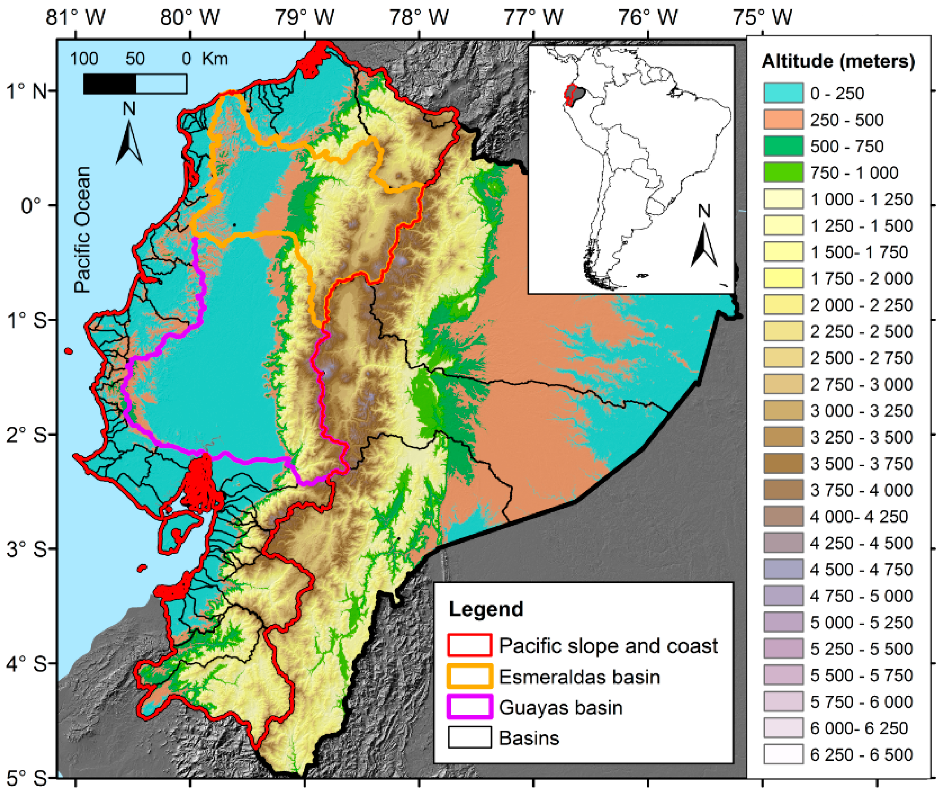
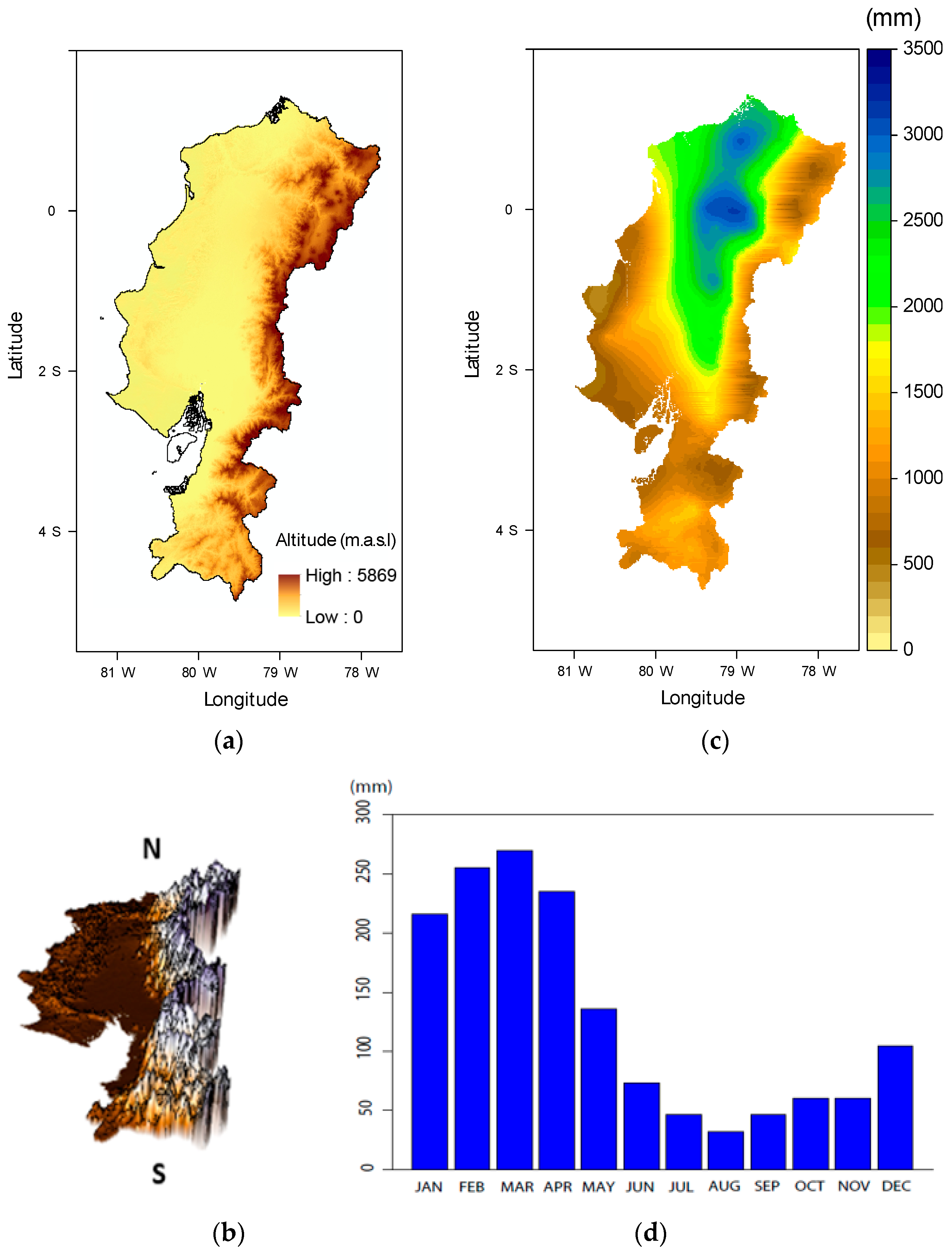
2. Study Area
3. Data
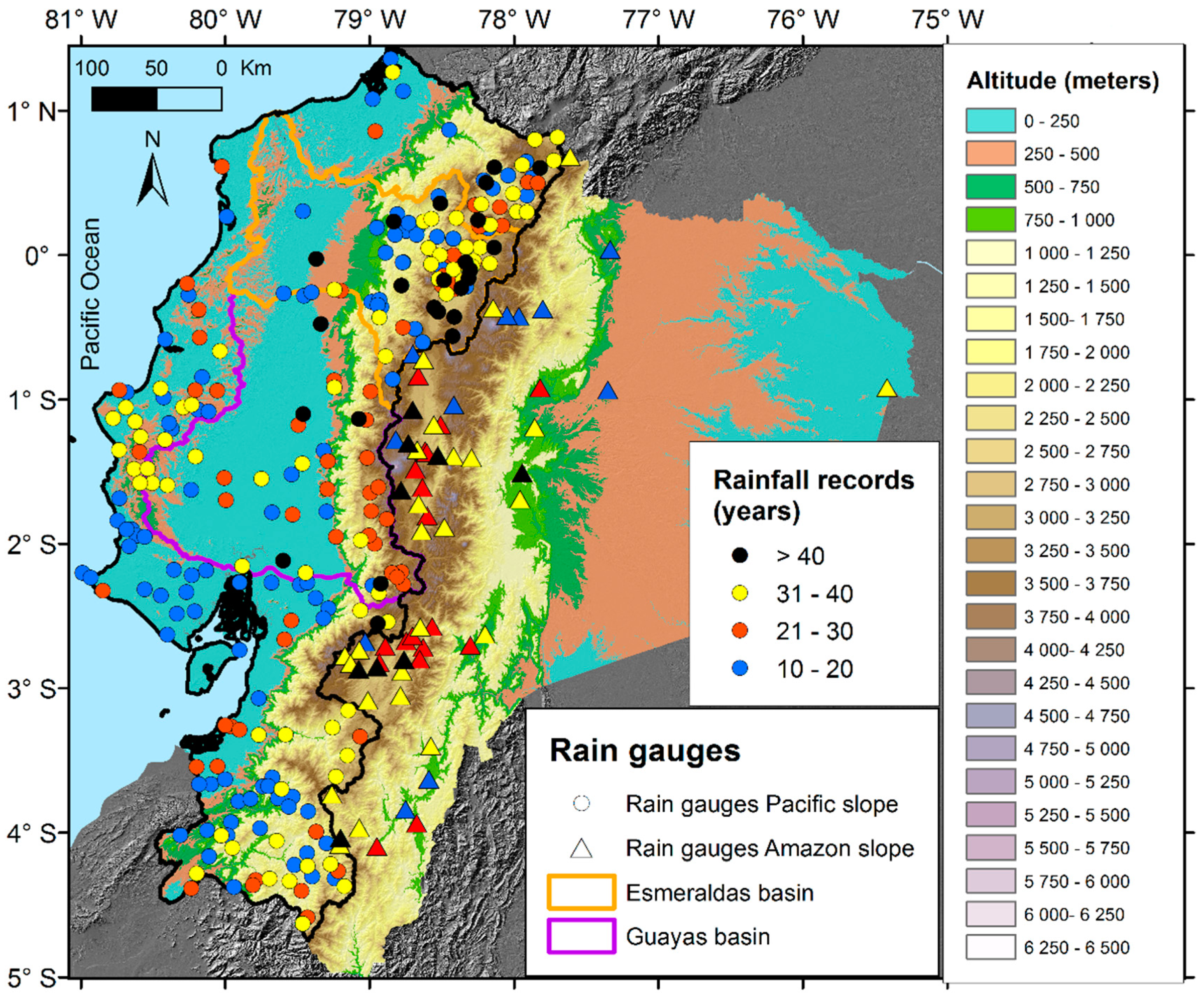
3.1. In Situ Rainfall Data
3.1.1. Data Homogenization and Validation
3.1.2. Rainfall Data Interpolation
3.2. Rainfall Products
4. Methods
4.1. Evaluation of the Rainfall Products
4.2. Evaluation of the Tropical Rainfall Measuring Mission (TRMM) Rainfall Product
5. Results
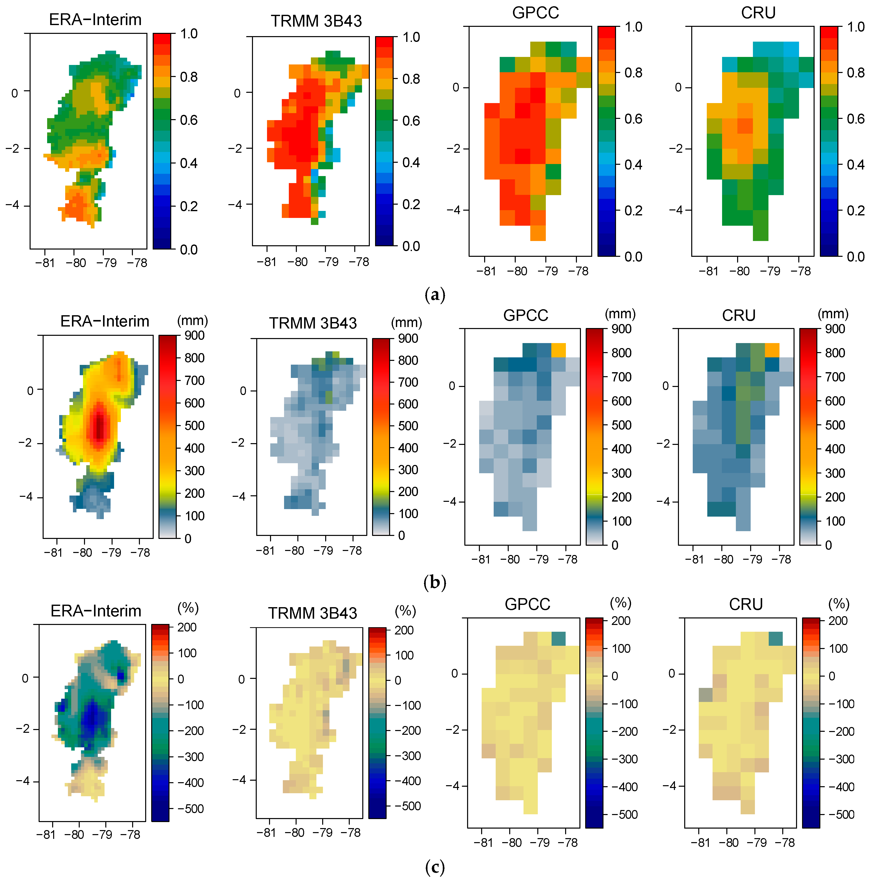
5.1. Rainfall Products Comparison
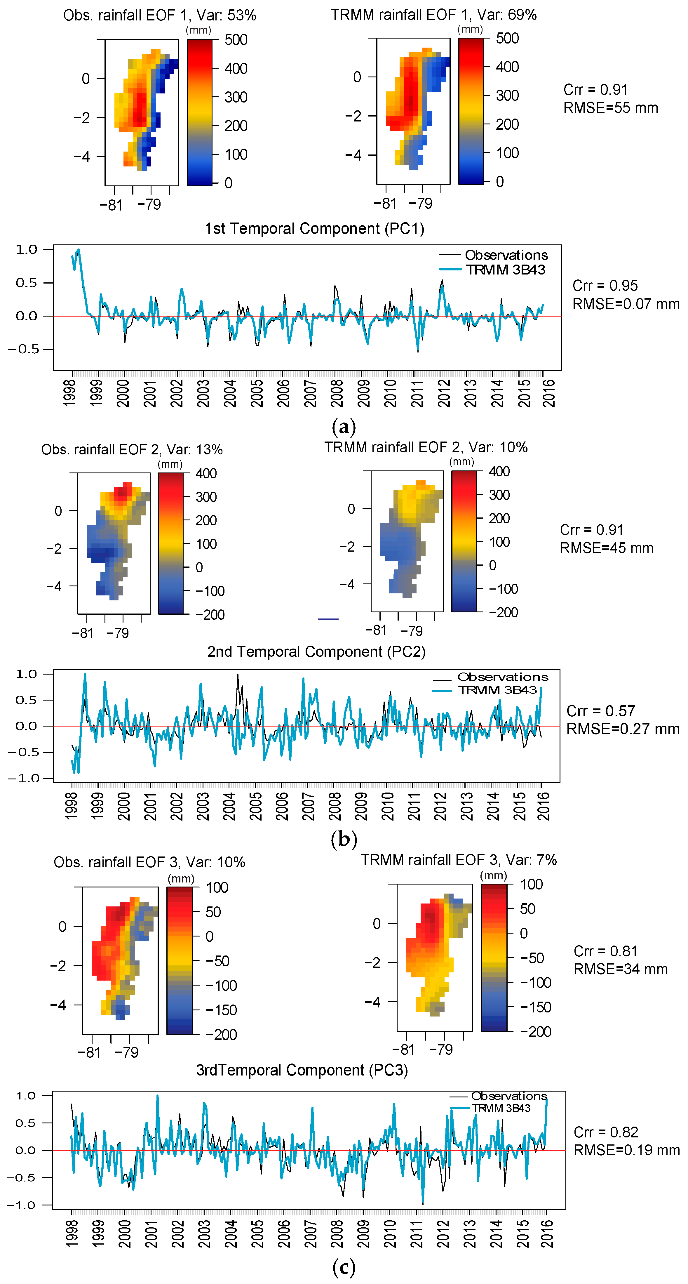
5.2. Identification of Spatio-Temporal Rainfall Variability with TRMM
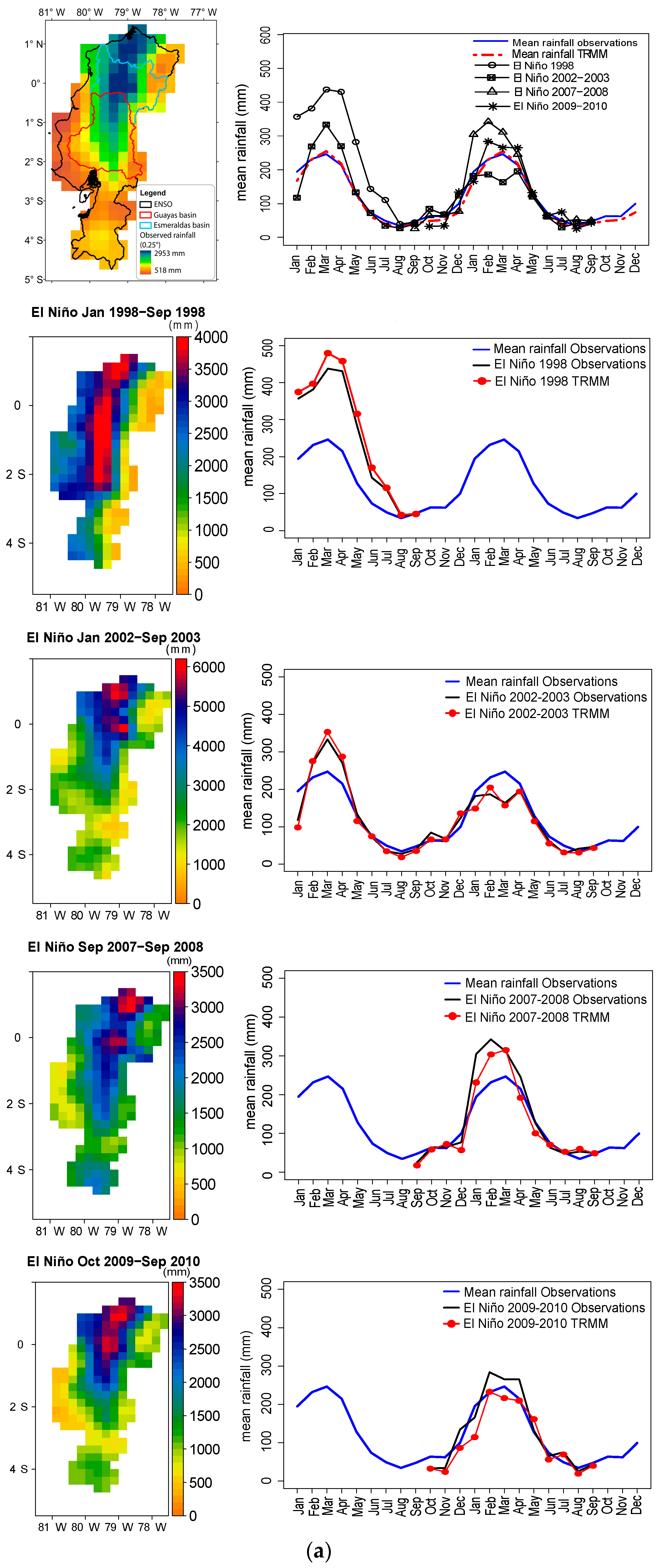
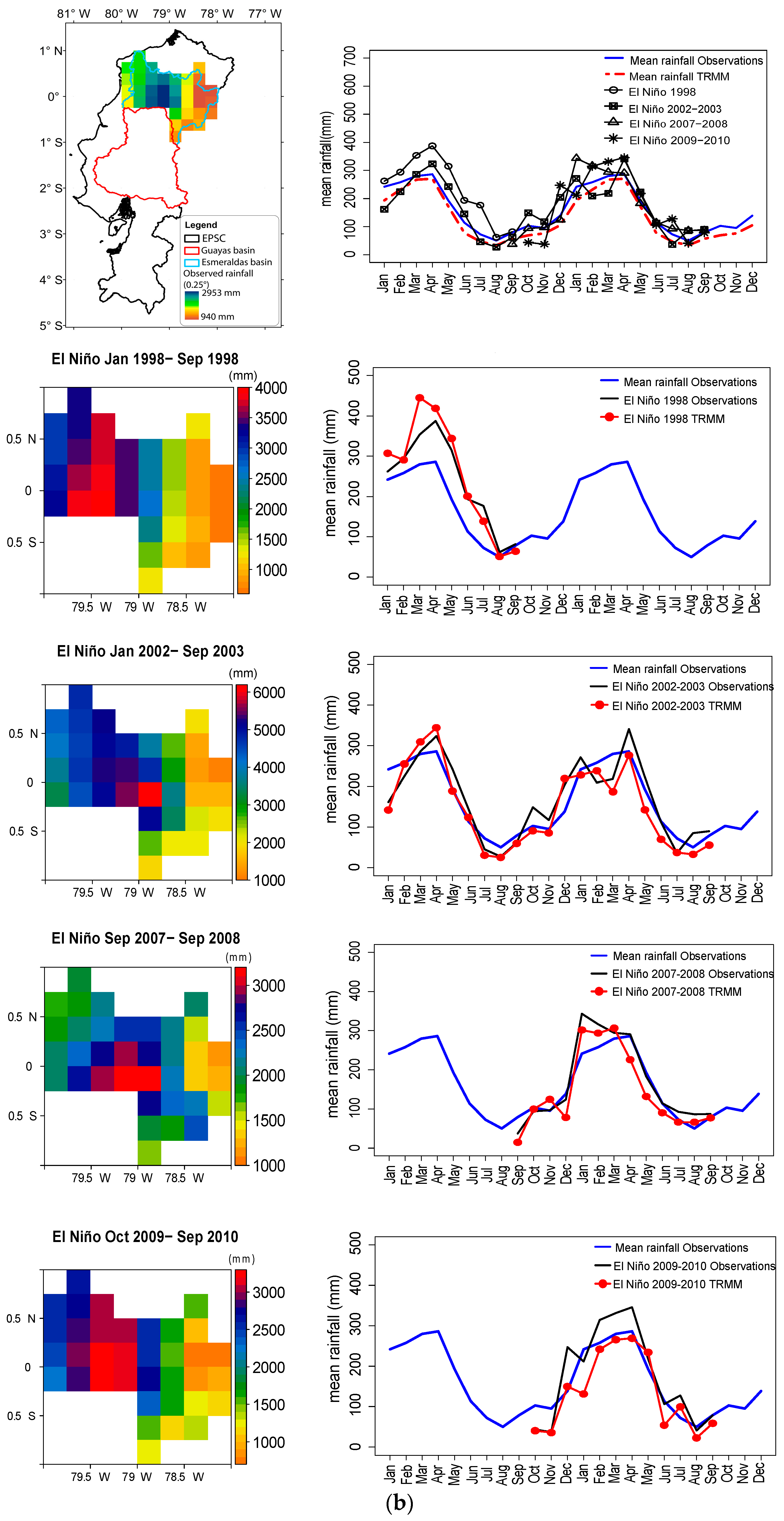
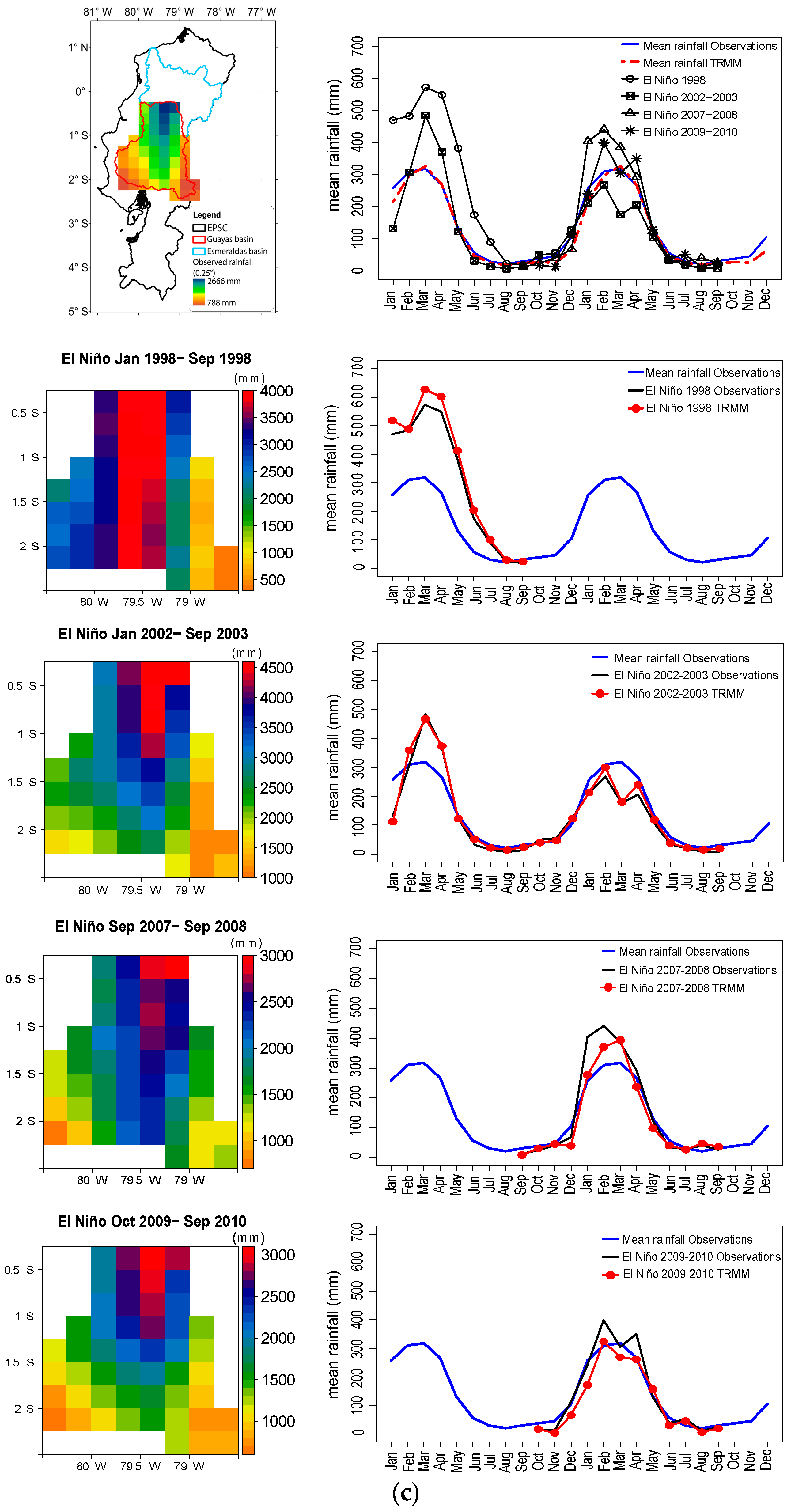
5.3. Identification of Spatio-Temporal Rainfall Variability during El Niño-Southern Oscillation (ENSO) Events with TRMM
5.3.1. Pacific Slope and Coast
5.3.2. Esmeraldas Basin
5.3.3. Guayas Basin
6. Discussion
7. Conclusions
Acknowledgments
Author Contributions
Conflicts of Interest
References
- Zhou, J.; Lau, K.M. Principal modes of interannual and decadal variability of summer rainfall over South America. Int. J. Climatol. 2001, 21, 1623–1644. [Google Scholar] [CrossRef]
- Haylock, M.R.; Peterson, T.C.; Alves, L.M.; Ambrizzi, T.; Anunciação, Y.M.T.; Baez, J.; Grimm, A.M.; Karoly, D.; Marengo, J.A.; Marino, M.B.; et al. Trends in Total and Extreme South American Rainfall in 1960–2000 and Links with. J. Clim. 2006, 19, 1490–1513. [Google Scholar] [CrossRef]
- Garreaud, R.D. The Andes climate and weather. Adv. Geosci. 2009, 7, 1–9. [Google Scholar] [CrossRef]
- Garreaud, R.D.; Vuille, M.; Compagnucci, R.; Marengo, J. Present-day South American climate. Palaeogeogr. Palaeoclimatol. Palaeoecol. 2009, 281, 180–195. [Google Scholar] [CrossRef]
- Vuille, M.; Bradley, R.S.; Keimig, F. Climate Variability in the Andes of Ecuador and Its Relation to Tropical Pacific and Atlantic Sea Surface Temperature Anomalies. J. Clim. 2000, 13, 2520–2535. [Google Scholar] [CrossRef]
- Mernild, S.H.; Liston, G.E.; Hiemstra, C.; Beckerman, A.P.; Yde, J.C.; Mcphee, J. The Andes Cordillera. Part IV: Spatio-temporal freshwater run-off distribution to adjacent seas (1979-2014). Int. J. Climatol. 2016. [Google Scholar] [CrossRef]
- Bendix, A.; Bendix, J. Heavy rainfall episodes in Ecuador during El Niño events and associated regional atmospheric circulation and SST patterns. Adv. Geosci. 2006, 6, 43–49. [Google Scholar] [CrossRef]
- Bendix, J.; Trache, K.; Palacios, E.; Rollenbeck, R.; Goettlicher, D.; Nauss, T.; Bendix, A. El Niño meets La Niña—Anomalous rainfall patterns in the “traditional” El Niño region of southern Ecuador. Erdkunde 2011, 65, 151–167. [Google Scholar] [CrossRef]
- Bendix, J.; Lauer, W. Die Niederschlagsjahreszeiten in Ecuador und ihre klimadynamische Interpretation (Rainy Seasons in Ecuador and Their Climate-Dynamic Interpretation). Erdkunde 1992, 46, 118–134. [Google Scholar] [CrossRef]
- Emck, P. A climatology of south Ecuador-with special focus on the major Andean ridge as Atlantic-Pacific climate divide. Ph.D. Thesis, Friedrich-Alexander-Universität Erlangen-Nürnberg (FAU), Erlangen, Germany, July 2007. [Google Scholar]
- Rollenbeck, R.; Bendix, J. Rainfall distribution in the Andes of southern Ecuador derived from blending weather radar data and meteorological field observations. Atmos. Res. 2011, 99, 277–289. [Google Scholar] [CrossRef]
- Bolvin, D.T.; Huffman, G.J. Transition of 3B42/3B43 research product from monthly to climatological calibration/adjustment. In NASA Precipitation Measurement Missions Document; NASA: Washington, DC, USA, 2015; pp. 1–11. [Google Scholar]
- Rossel, F.; Mejía, R.; Ontaneda, G.; Pombosa, R.; Roura, J.; Calvez, R.; Cadier, E. Régionalisation de l’influence du El Niño sur les précipitations de l’Equateur. Bulletin d'Institut Français D'études Andines 1998, 27, 643–654, ISSN:0303-7495. [Google Scholar]
- Morán-Tejeda, E.; Bazo, J.; López-Moreno, J.I.; Aguilar, E.; Azorín-Molina, C.; Sanchez-Lorenzo, A.; Martínez, R.; Nieto, J.J.; Mejía, R.; Martín-Hernández, N.; et al. Climate trends and variability in Ecuador (1966–2011). Int. J. Climatol. 2015. [Google Scholar] [CrossRef]
- Lavado, W.; Labat, D.; Guyot, J.L.; Ronchail, J.; Ordoñez, J. TRMM rainfall data estimation over the Peruvian Amazon-Andes basin and its assimilation into a monthly water balance model. In New Approaches to Hydrological Prediction in Data-Sparse Regions; International Association of Hydrological Sciences: London, UK, 2009. [Google Scholar]
- Condom, T.; Rau, P.; Espinoza, J.C. Correction of TRMM 3B43 monthly precipitation data over the mountainous areas of Peru during the period 1998-2007. Hydrol. Process. 2011, 25, 1924–1933. [Google Scholar] [CrossRef]
- Mantas, V.M.; Liu, Z.; Caro, C.; Pereira, A.J.S.C. Validation of TRMM multi-satellite precipitation analysis (TMPA) products in the Peruvian Andes. Atmos. Res. 2014. [Google Scholar] [CrossRef]
- Scheel, M.L.M.; Rohrer, M.; Huggel, C.; Villar, D.S.; Silvestre, E.; Huffman, G.J. Evaluation of TRMM Multi-satellite Precipitation Analysis (TMPA ) performance in the Central Andes region and its dependency on spatial and temporal resolution. Hydrol. Earth Syst. Sci. 2011, 2649–2663. [Google Scholar] [CrossRef] [Green Version]
- Franchito, S.H.; Rao, V.B.; Vasques, A.C.; Santo, C.M.E.; Conforte, J.C. Validation of TRMM precipitation radar monthly rainfall estimates over Brazil. J. Geophys. Res. Atmos. 2009, 114. [Google Scholar] [CrossRef]
- Negrón Juárez, R.I.; Li, W.; Fu, R.; Fernandes, K.; de Oliveira Cardoso, A. Comparison of Precipitation Datasets over the Tropical South American and African Continents. J. Hydrometeorol. 2009, 10, 289–299. [Google Scholar] [CrossRef]
- Zulkafli, Z.; Buytaert, W.; Onof, C.; Manz, B.; Tarnavsky, E.; Lavado, W.; Guyot, J.-L. A Comparative Performance Analysis of TRMM 3B42 (TMPA) Versions 6 and 7 for Hydrological Applications over Andean–Amazon River Basins. J. Hydrometeorol. 2014, 15, 581–592. [Google Scholar] [CrossRef]
- Frappart, F.; Ramillien, G.; Ronchail, J. Changes in terrestrial water storage versus rainfall and discharges in the Amazon basin. Int. J. Climatol. 2013, 33, 3029–3046. [Google Scholar] [CrossRef] [Green Version]
- Bendix, J.; Rollenbeck, R.; Reudenbach, C. Diurnal patterns of rainfall in a tropical Andean valley of southern Ecuador as seen by a vertically pointing K-band Doppler radar. Int. J. Climatol. 2006, 26, 829–846. [Google Scholar] [CrossRef]
- Pfafstetter, O. Classification of hydrographic basins: Coding methodology. Unpublished work. 1989. [Google Scholar]
- Bourrel, L.; Melo, P.; Vera, A.; Pombosa, R.; Guyot, J.L. Study of the erosion risks of the Ecuadorian Pacific coast under the influence of ENSO phenomenom: Case of the Esmeraldas and Guayas basins. In Proceedings of the International Conference on the Status and Future of the World’s Large Rivers, Vienna, Austria, 11–14 April 2011; pp. 11–14. [Google Scholar]
- Frappart, F.; Bourrel, L.; Brodu, N.; Riofrío Salazar, X.; Baup, F.; Darrozes, J.; Pombosa, R. Monitoring of the Spatio-Temporal Dynamics of the Floods in the Guayas Watershed (Ecuadorian Pacific Coast) Using Global Monitoring ENVISAT ASAR Images and Rainfall Data. Water 2017, 9, 12. [Google Scholar] [CrossRef]
- Bourrel, L.; Rau, P.; Dewitte, B.; Labat, D.; Lavado, W.; Coutaud, A.; Vera, A.; Alvarado, A.; Ordoñez, J. Low-frequency modulation and trend of the relationship between ENSO and precipitation along the northern to centre Peruvian Pacific coast. Hydrol. Process. 2014, 29, 1252–1266. [Google Scholar] [CrossRef]
- Rau, P.; Bourrel, L.; Labat, D.; Melo, P.; Dewitte, B.; Frappart, F.; Lavado, W.; Felipe, O. Regionalization of rainfall over the Peruvian Pacific slope and coast. Int. J. Climatol. 2016. [Google Scholar] [CrossRef]
- Brunet Moret, Y. Homogénéisation des précipitations. ORSTOM 1979, XVI, 147–170. [Google Scholar]
- Cressie, N.; Johannesson, G. Fixed rank kriging for very large spatial data sets. J. R. Stat. Soc. Ser. B Stat. Methodol. 2008, 70, 209–226. [Google Scholar] [CrossRef]
- Jarvis, A.; Reuter, H.I.; Nelson, A.; Guevara, E.; others Hole-filled SRTM for the globe Version 4. Available CGIAR-CSI SRTM 90m Database Httpsrtm Csi Cgiar Org. 2008. Available online: http://www.cgiar-csi.org/data/srtm-90m-digital-elevation-database-v4-1 (accessed on 15 May 2017).
- Hijmans, R.J.; van Etten, J. Raster: Geographic data analysis and modeling. R Package Version 2014, 2, 15. [Google Scholar]
- Pebesma, E. spacetime : Spatio-Temporal Data in R. J. Stat. Softw. 2012, 51, 1–30. [Google Scholar] [CrossRef]
- Hiemstra, P.; Hiemstra, M.P. Package “automap”. Compare 2013, 105, 10. [Google Scholar]
- Schuurmans, J.M.; Bierkens, M.F.P.; Pebesma, E.J.; Uijlenhoet, R. Automatic Prediction of High-Resolution Daily Rainfall Fields for Multiple Extents: The Potential of Operational Radar. J. Hydrometeorol. 2007, 8, 1204–1224. [Google Scholar] [CrossRef]
- Buytaert, W.; Celleri, R.; Willems, P.; De Bièvre, B.; Wyseure, G. Spatial and temporal rainfall variability in mountainous areas: A case study from the south Ecuadorian Andes. J. Hydrol. 2006, 329, 413–421. [Google Scholar] [CrossRef] [Green Version]
- Diodato, N. The influence of topographic co-variables on the spatial variability of precipitation over small regions of complex terrain. Int. J. Climatol. 2005, 25, 351–363. [Google Scholar] [CrossRef]
- Mourre, L.; Condom, T.; Junquas, C.; Lebel, T.; Sicart, J.E.; Figueroa, R.; Cochachin, A. Spatio-temporal assessment of WRF, TRMM and in situ precipitation data in a tropical mountain environment (Cordillera Blanca, Peru). Hydrol. Earth Syst. Sci. 2016, 20, 125–141. [Google Scholar] [CrossRef]
- Cressman, G.P. An Operational Objective Analysis System. Mon. Weather Rev. 1959, 87, 367–374. [Google Scholar] [CrossRef]
- Mitchell, T.P.; Wallace, J.M. The annual cycle in equatorial convection and sea surface temperature. J. Clim. 1992, 5, 1140–1156. [Google Scholar] [CrossRef]
- Schneider, U.; Ziese, M.; Meyer-Christoffer, A.; Finger, P.; Rustemeier, E.; Becker, A. The new portfolio of global precipitation data products of the Global Precipitation Climatology Centre suitable to assess and quantify the global water cycle and resources. Proc. Int. Assoc. Hydrol. Sci. 2016, 374, 29–34. [Google Scholar] [CrossRef]
- Harris, I.; Jones, P.D.; Osborn, T.J.; Lister, D.H. Updated high-resolution grids of monthly climatic observations–the CRU TS3. 10 Dataset. Int. J. Climatol. 2014, 34, 623–642. [Google Scholar] [CrossRef] [Green Version]
- Dee, D.P.; Uppala, S.M.; Simmons, A.J.; Berrisford, P.; Poli, P.; Kobayashi, S.; Andrae, U.; Balmaseda, M.A.; Balsamo, G.; Bauer, P.; et al. The ERA-Interim reanalysis: Configuration and performance of the data assimilation system. Q. J. R. Meteorol. Soc. 2011, 137, 553–597. [Google Scholar] [CrossRef]
- Huffman, G.J.; Bolvin, D.T. TRMM and Other Data Precipitation Data Set Documentation; TRMM 3B423B43 Doc; NASA: Greenbelt, MD, USA, 2015; pp. 1–44. [CrossRef]
- Jolliffe, I.T.; Cadima, J. Principal component analysis: A review and recent developments. Phil. Trans. R. Soc. A 2016, 374. [Google Scholar] [CrossRef] [PubMed]
- Preisendorfer, R.W.; Mobley, C.D. Principal Component Analysis in Meteorology and Oceanography; Elsevier: Amsterdam, The Netherlands, 1988; Volume 425. [Google Scholar]
- Southern Oscillation Index (SOI) | Teleconnections | National Centers for Environmental Information (NCEI). Available online: https://www.ncdc.noaa.gov/teleconnections/enso/indicators/soi/ (accessed on 27 July 2017).
- Null, J. El Nino and La Nina Years and Intensities Based on Oceanic Nino index (ONI); NOAA: Silver Spring, MD, USA, 2015.
- Huang, B.; Banzon, V.F.; Freeman, E.; Lawrimore, J.; Liu, W.; Peterson, T.C.; Smith, T.M.; Thorne, P.W.; Woodruff, S.D.; Zhang, H.-M. Extended reconstructed sea surface temperature version 4 (ERSST. v4). Part I: Upgrades and intercomparisons. J. Clim. 2015, 28, 911–930. [Google Scholar] [CrossRef]
- Schneider, U.; Becker, A.; Finger, P.; Meyer-Christoffer, A.; Ziese, M.; Rudolf, B. GPCC’s new land surface precipitation climatology based on quality-controlled in situ data and its role in quantifying the global water cycle. Theor. Appl. Climatol. 2014, 115, 15–40. [Google Scholar] [CrossRef]
- Maidment, R.I.; Grimes, D.I.F.; Allan, R.P.; Greatrex, H.; Rojas, O.; Leo, O. Evaluation of satellite-based and model re-analysis rainfall estimates for Uganda. Meteorol. Appl. 2013, 20, 308–317. [Google Scholar] [CrossRef]
- Norina, A.; Vegas, F.; Lavado, C. Zappa water resources and climate change impact modelling on a daily time scale in the Peruvian Andes. Hydrol. Sci. J. 2014, 59, 2043–2059. [Google Scholar] [CrossRef]
- Ballari, D.; Castro, E.; Campozano, L. Validation of Satellite Precipitation (TRMM 3B43) in Ecuadorian Coastal Plains, Andean Highlands and Amazonian Rainforest. ISPRS-Int. Arch. Photogramm. Remote Sens. Spat. Inf. Sci. 2016, 305–311. [Google Scholar]
- Satgé, F.; Bonnet, M.-P.; Gosset, M.; Molina, J.; Lima, W.H.Y.; Zolá, R.P.; Timouk, F.; Garnier, J. Assessment of satellite rainfall products over the Andean plateau. Atmos. Res. 2016, 167, 1–14. [Google Scholar] [CrossRef]
- Manz, B.; Buytaert, W.; Zulkafli, Z.; Lavado, W.; Willems, B.; Robles, L.A.; Rodríguez-Sánchez, J.-P. High-resolution satellite-gauge merged precipitation climatologies of the Tropical Andes. J. Geophys. Res. Atmos. 2016. [Google Scholar] [CrossRef]
- Dinku, T.; Connor, S.J.; Ceccato, P. Comparison of CMORPH and TRMM-3B42 over mountainous regions of Africa and South America. In Satellite Rainfall Applications for Surface Hydrology; Springer: Berlin, Germany, 2010; pp. 193–204. [Google Scholar]
- Espinoza, J.C.; Chavez, S.; Ronchail, J.; Junquas, C.; Takahashi, K.; Lavado, W. Rainfall hotspots over the southern tropical Andes: Spatial distribution, rainfall intensity, and relations with large-scale atmospheric circulation. Water Resour. Res. 2015, 51, 3459–3475. [Google Scholar] [CrossRef]
- Levizzani, V.; Amorati, R.; Meneguzzo, F. A Review of Satellite-Based Rainfall Estimation Methods. In MUSIC–MUltiple-Sensor Precipitation Measurements, Integration, Calibration and Flood Forecasting; European Commission: Brussels, Belgium, 2002; Volume 70. [Google Scholar]
- Mätzler, C.; Standley, A. Technical note: Relief effects for passive microwave remote sensing. Int. J. Remote Sens. 2000, 21, 2403–2412. [Google Scholar] [CrossRef]
- North, G.R.; Bell, T.L.; Cahalan, R.F.; Moeng, F.J. Sampling errors in the estimation of empirical orthogonal functions. Mon. Weather Rev. 1982, 110, 699–706. [Google Scholar] [CrossRef]
- Bendix, J.; Rollenbeck, R.; Göttlicher, D.; Cermak, J. Cloud occurrence and cloud properties in Ecuador. Clim. Res. 2006, 30, 133–147. [Google Scholar] [CrossRef]
- Diaz, H.F.; Markgraf, V. El Niño and the Southern Oscillation: Multiscale Variability and Global and Regional Impacts; Cambridge University Press: Cambridge, UK, 2000. [Google Scholar]
- Campozano, L.; Célleri, R.; Trachte, K.; Bendix, J.; Samaniego, E. Rainfall and Cloud Dynamics in the Andes: A Southern Ecuador Case Study. Adv. Meteorol. 2016, 2016. [Google Scholar] [CrossRef]
- Philander, S.G.H.; El Niño, L.N. The Southern Oscillation; Academic Press: San Diego, CA, USA, 1990; pp. 904–905. [Google Scholar]
- Schneider, T.; Bischoff, T.; Haug, G.H. Migrations and dynamics of the intertropical convergence zone. Nature 2014, 513, 45–53. [Google Scholar] [CrossRef] [PubMed]
- Arteaga, K.; Tutasi, P.; Jiménez, R. Climatic variability related to El Niño in Ecuador? A historical background. Adv. Geosci. 2006, 6, 237–241. [Google Scholar] [CrossRef]
- Dai, A.; Wigley, T.M.L. Global patterns of ENSO-induced precipitation. Geophys. Res. Lett. 2000, 27, 1283–1286. [Google Scholar] [CrossRef]
- Iguchi, T.; Kozu, T.; Meneghini, R.; Awaka, J.; Okamoto, K. Rain-profiling algorithm for the TRMM precipitation radar. J. Appl. Meteorol. 2000, 39, 2038–2052. [Google Scholar] [CrossRef]
- Rasmussen, K.L.; Choi, S.L.; Zuluaga, M.D.; Houze, R.A. TRMM precipitation bias in extreme storms in South America. Geophys. Res. Lett. 2013, 40, 3457–3461. [Google Scholar] [CrossRef]
- Nastos, P.T.; Kapsomenakis, J.; Philandras, K.M. Evaluation of the TRMM 3B43 gridded precipitation estimates over Greece. Atmos. Res. 2016, 169, 497–514. [Google Scholar] [CrossRef]
- Sorooshian, S.; Hsu, K.-L.; Gao, X.; Gupta, H.V.; Imam, B.; Braithwaite, D. Evaluation of PERSIANN system satellite–based estimates of tropical rainfall. Bull. Am. Meteorol. Soc. 2000, 81, 2035–2046. [Google Scholar] [CrossRef]
- Islam, M.N.; Uyeda, H. Use of TRMM in determining the climatic characteristics of rainfall over Bangladesh. Remote Sens. Environ. 2007, 108, 264–276. [Google Scholar] [CrossRef]
- Stano, G.; Krishnamurti, T.N.; Kumar, T.V.; Chakraborty, A. Hydrometeor structure of a composite monsoon depression using the TRMM radar. Tellus A 2002, 54, 370–381. [Google Scholar] [CrossRef]
- Lau, K.M.; Wu, H.T. Warm rain processes over tropical oceans and climate implications. Geophys. Res. Lett. 2003, 30. [Google Scholar] [CrossRef]
- Dinku, T.; Ceccato, P.; Connor, S.J. Challenges of satellite rainfall estimation over mountainous and arid parts of east Africa. Int. J. Remote Sens. 2011, 32, 5965–5979. [Google Scholar] [CrossRef]


| Product and Version | Spatial Resolution | Time Period Available | Source and Reference | Using Period (Common Period) |
|---|---|---|---|---|
| Ecuadorian rain gauges | ||||
| Interpolated Rainfall (Cokring) | 5 km (0.04°) | 1965–2015 | Meteorological and Hydrological National Institute of Ecuador (INAMHI) | 1970–2015 |
| Global rain-gauge dataset | ||||
| GPCC, v7 | 0.5° | 1901–2013 | Global Precipitation Climatology Centre (GPCC), National Meteorological Service of Germany [41] | 1970–2013 |
| CRU, v3.22 | 0.5° | 1901–2013 | Climate Research Unit (CRU), University of East Anglia [42] | 1970–2013 |
| Reanalysis | ||||
| ERA-Interim (Synoptic monthly mean) | 0.125° | 1979–present | European Centre for Medium-Range Weather Forecasts (ECMWF) [43] | 1979–2015 |
| Satellite | ||||
| Tropical Rainfall Measuring Mission (TRMM) 3B43 V7 | 0.25° | 1998–2015 | National Aeronautics and Space Administration (NASA) Goddard Space Flight Centre [44] | 1998–2015 |
| Rainfall Source | Compared Times Series | Resolution (Degrees) | Mean Annual Precipitation (mm/year) and Difference with Observations in % (in Parenthesis) | Mean Correlation with Obs | Mean RMSE with Obs (mm/year) | Mean of Relative Bias Index (Rbias) (%) with Respect to Observations |
|---|---|---|---|---|---|---|
| Interpolated observations (COK) | Common periods respectively | 0.008 | 1537.1 | |||
| ERA-Interim Total precipitation | 1979–2015 | 0.125 | 4117.4 (+167.9%) | 0.69 | 288.2 | −177.1 |
| TRMM 3B43 V7 | 1998–2014 | 0.25 | 1345.5 (−12.5%) | 0.82 | 68.7 | −2.8 |
| GPCC V7 | 1970–2013 | 0.5 | 1331.8 (−13.4%) | 0.83 | 69.8 | 5.7 |
| CRU V3.22 | 1970–2013 | 0.5 | 1468.2 (−4.5%) | 0.66 | 102.3 | −2.3 |
| Time Period | Ecuadorian Pacific Slope and Coast | Esmeraldas Basin | Guayas Basin | |||
|---|---|---|---|---|---|---|
| Observed Rainfall Event with Respect to the Average (%) | TRMM Estimation of Observed Rainfall (%) | Observed Rainfall Event with Respect to the Average | TRMM Estimation of Observed Rainfall (%) | Observed Rainfall Event with Respect to the Average | TRMM Estimation of Observed Rainfall (%) | |
| Available period: Jan 1998–Dec 2015 | −6.9 | −16.4 | −8.5 | |||
| ENSO: Jan 1998–Sep 1998 | 75.1 | 7.7 | 43.2 | 6.3 | 100.7 | 8.5 |
| ENSO: Jan 2002–Sep 2003 | −3.5 | −2.4 | 3.4 | −12 | −21.3 | 5.3 |
| ENSO: Sep 2007–Sep 2008 | 9.3 | −11 | 8.1 | −13.1 | 0.8 | −14.2 |
| ENSO: Oct 2009–Sep 2010 | −0.8 | −17.1 | 5.9 | −23.7 | −7.5 | −18.9 |
© 2018 by the authors. Licensee MDPI, Basel, Switzerland. This article is an open access article distributed under the terms and conditions of the Creative Commons Attribution (CC BY) license (http://creativecommons.org/licenses/by/4.0/).
Share and Cite
Erazo, B.; Bourrel, L.; Frappart, F.; Chimborazo, O.; Labat, D.; Dominguez-Granda, L.; Matamoros, D.; Mejia, R. Validation of Satellite Estimates (Tropical Rainfall Measuring Mission, TRMM) for Rainfall Variability over the Pacific Slope and Coast of Ecuador. Water 2018, 10, 213. https://doi.org/10.3390/w10020213
Erazo B, Bourrel L, Frappart F, Chimborazo O, Labat D, Dominguez-Granda L, Matamoros D, Mejia R. Validation of Satellite Estimates (Tropical Rainfall Measuring Mission, TRMM) for Rainfall Variability over the Pacific Slope and Coast of Ecuador. Water. 2018; 10(2):213. https://doi.org/10.3390/w10020213
Chicago/Turabian StyleErazo, Bolívar, Luc Bourrel, Frédéric Frappart, Oscar Chimborazo, David Labat, Luis Dominguez-Granda, David Matamoros, and Raul Mejia. 2018. "Validation of Satellite Estimates (Tropical Rainfall Measuring Mission, TRMM) for Rainfall Variability over the Pacific Slope and Coast of Ecuador" Water 10, no. 2: 213. https://doi.org/10.3390/w10020213