Impact of Climate Change on Water Resources of the Bheri River Basin, Nepal


1
School of Engineering and Technology, Asian Institute of Technology, PO Box 4, Klong Luang, 12120 Pathumathani, Thailand
2
Geoinformatics Center, Asian Institute of Technology, PO Box 4, Klong Luang, 12120 Pathumathani, Thailand
*
Author to whom correspondence should be addressed.
Water 2018, 10(2), 220; https://doi.org/10.3390/w10020220
Submission received: 19 November 2017
/
Revised: 31 January 2018
/
Accepted: 7 February 2018
/
Published: 18 February 2018
Abstract
:Streamflow alteration is one of the most noticeable effects of climate change. This study explored the effects of climate change on streamflow in the Bheri River using the Soil and Water Assessment Tool (SWAT) model. Three General Circulation Models (GCMs) under two Representative Concentration Pathways (RCPs; 4.5 and 8.5) for the periods of 2020–2044, 2045–2069, and 2070–2099 were used to investigate the impact of climate change. Based on the ensemble of the three models, we observed an increasing trend in maximum and minimum temperatures at the rate of 0.025 °C/year and 0.033 °C/year, respectively, under RCP 4.5, and 0.065 °C/year and 0.071 °C/year under RCP 8.5 in the future. Similarly, annual rainfall will increase by 6.8–15.2% in the three future periods. The consequences of the increment in rainfall and temperature are reflected in the annual streamflow that is projected to increase by 6–12.5% when compared to the historical data of 1975–2005. However, on a monthly scale, runoff will decrease in July and August by up to 20% and increase in the dry period by up to 70%, which is favorable for water users.
1. Introduction
The Fifth Assessment Report of the Intergovernmental Panel on Climate Change (IPCC AR5, 2014) mentions that the entire earth’s temperature increased by 0.85 °C from 1881 to 2012 and for each of the recent past three decades, every consecutive decade has been hotter than the previous one [1]. Large areas of the Himalayan river basins are covered by snow and glaciers and are, therefore, more vulnerable to climate change [2]. Many studies have shown that the temperature in the Himalayan basins is showing an increasing trend [3,4]. Such a phenomenon will alter water availability in rivers, especially in autumn and spring. Many researchers anticipate that the average temperature of Nepal will increase by 5.8 °C by 2100, with more pronounced warming at higher altitudes [5]. A study carried out by Immerzeel et al. [6] in the Langtang Watershed of the Ganges River and the Baltoro Watershed of the Indus River concluded that water availability during this century was not likely to decline. This is due to the rise in glacier melt runoff as well as an increase in rainfall and similar scenarios that can also be seen in other Himalayan catchments. The study showed that the water holding capacity of air will increase by about 7% per 1 °C increment, which will lead to increased water vapor in the atmosphere [7]. This, consequently, will produce more frequent and intense rainfall events. It will affect streamflow patterns on a basin scale, which was our focus in this study.
A General Circulation Model (GCM) is a climate model that represents the general circulation of planetary atmosphere mathematically. These models can provide reliable information regarding historical, current, and future climate trends [8] over long periods. Generally, an ensemble of various GCMs can represent a range of possible scenarios which provide a better idea about possible future climate than just a single GCM [9]. Several researchers have applied the climate projections of an ensemble of three to six GCMs in hydro-climatic studies for future projections [10,11,12]. However, the spatial resolution of a GCM is very coarse, which makes it incompatible with local hydrological models. To fill this gap, a downscaling method can be used as a bridge. Regional Climate Model (RCM) is available in relatively higher spatial resolutions than GCM. Furthermore, RCM can be placed within a GCM to provide more detailed simulation. RCM covers a smaller area with better resolution, which requires more intensive computation to run it, and is appropriate for mountainous and coastal areas.
The Coupled Model Inter comparison Project Phase 5 (CMIP5) developed climate change scenarios called Representative Concentration Pathways (RCPs) [13], which project possible climate scenarios in the future. Studies have shown that RCP scenarios are an appropriate approach for investigations of future climatic conditions, and the results are used to perform the impact analysis of climate change and plan mitigation measures [14].
Hydrological models are often used to simulate future hydrological cycles and GCM-projected temperature and rainfall data are used to force these models. There are many criteria that are applied to select an appropriate hydrological model. The spatial scale of the model, the flexibility of testing different weather conditions, the ease of amendment with different data sets, the objective of the study, the hydrological processes represented in the structure of the model, and the ease of calibration are the key measures of a hydrological model. The Soil and Water Assessment Tools (SWAT) is a process-based semi-distributed hydrological model that can simulate the discharge under future scenarios, consequently able to predict the impact of climate change on the hydrological and biogeochemical cycles in a variety of watersheds. However, the prediction depends on the quality of the input data. The SWAT model has been used extensively in many river basins to predict the impacts of climate change such as in the Kelantan River Basin in Malaysia [15], the Koshi River Basin in Nepal [16], and the Great Lakes Watershed [17], etc. Locally in Nepal, SWAT has been applied to study the impact of climate change in various watershed studies such as the Indravati [18], West Seti Basin [19], and the Bagmati [20].
The Bheri River Basin (BRB) is an important river basin in the western part of Nepal as this river is the only snow-fed river from which water can be easily transferred to the south-western belt of the country [21]. The Nepalese government is building a project to transfer water from this river to the Babai River. The Babai River Basin is a water deficit basin and the Bheri River is the only probable donor river [22]. After the water transfer is complete, an additional 50,000 ha (hectare) of land will receive year-round irrigation in the Babai River Basin [21]. The data of the impact of climate change on the streamflow of the BRB will be valuable and essential for managing water resources and facilitating regional development in western Nepal. As of now, it appears that no research has been conducted in the BRB related to the assessment of the impacts of climate change. This study addresses this gap and examines the impact of climate change on the streamflow of the Bheri River. The Statistical Downscaling Method (SDSM) was employed to acquire data from the three selected GCMs. Streamflow features were compared in three future periods 2020–2044 (30 s), 2045–2069 (60 s), and 2070–2099 (80 s) for RCP 4.5 and RCP 8.5.
The main objective of this study was to carry out an extensive analysis of streamflow under different climate change scenarios using the SWAT model in the BRB. Three GCMs (as part of an ensemble), two RCPs, and three future periods were selected, which created twenty-four scenarios for projection. The most important aspects of this work include: (i) projecting future temperatures and rainfall from the data of the three GCMs by using the SDSM method; (ii) projecting future streamflow from the calibrated SWAT model by using downscaled outputs; and (iii) analyzing the streamflow result obtained from different GCMs under different future scenarios.
The findings from this study will help water management strategies in the BRB and other river basins that have similar climatic and topographic characteristics. Furthermore, the projected water cycle component could be used in other applications such as water diversion and the modeling of ecological changes.
2. Study Area
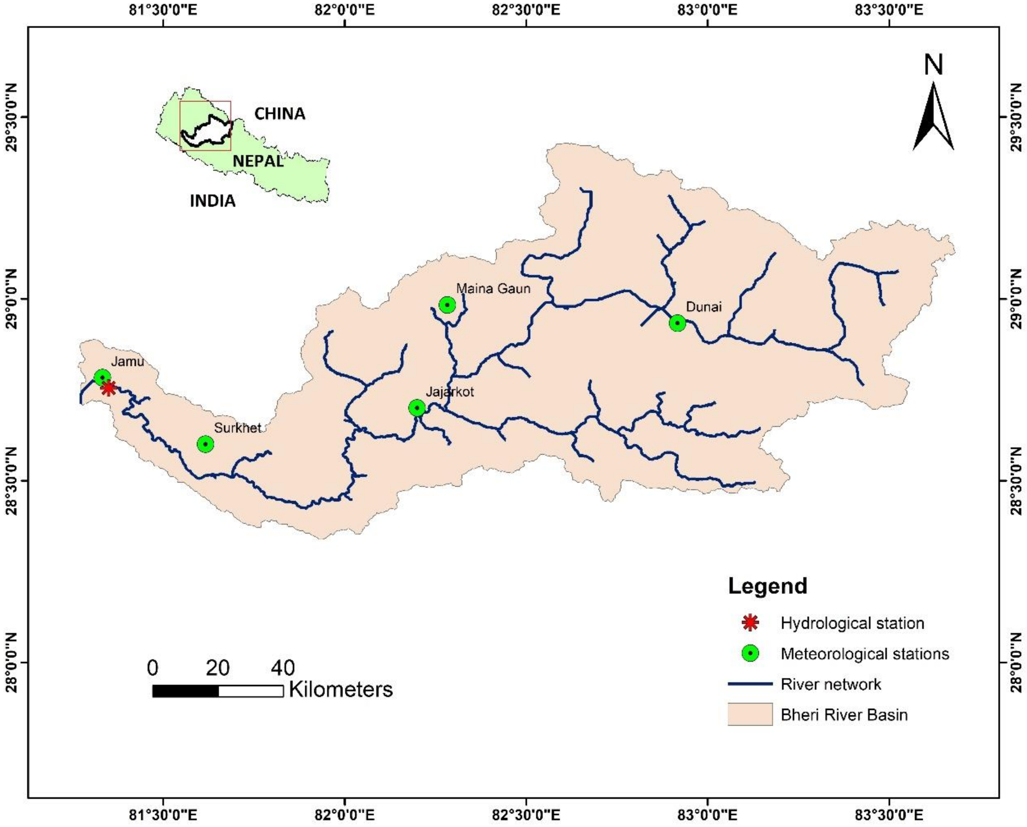
The Bheri River Basin (BRB) (13,900 km2) (Figure 1) is one of the major tributaries of the Karnali River, the third largest river system of Nepal. The Bheri River is about 264 km long and extends between latitudes 28°20′ N to 29°25′ N and longitudes 81°16′ E to 83°41′ E. The elevation varies from 200 to 7746 m with permanent snowcapped mountains such as the western Dhaulagiri range in the north. The Little Bheri, the Big Bheri, and the Uttar Ganga are the three tributaries of the Bheri River. The Big Bheri flows to the northern slope, the Small Bheri to the southern slope, and the Uttar Ganga flows through the Dhorpatan Valley, famous for being the only hunting reserve in Nepal, to the south of Dhaulagiri. The Bheri River flows to the nearby city of Surkhet and joins the Karnali River within the Mahabharata range.
As it is very common having low density of climatological station is in developing county such as Nepal. Due to its very difficult topography, setting up of climatological and hydrological stations was not in priority in Bheri River Basin (BRB). In about 13,900 km2 of basin area, there are only five climatological stations. All stations are in the lower altitude because higher altitude area is inaccessible due to remoteness of geography. The data obtained from the Department of Hydrology and Meteorology, Nepal, from 1975–2005 shows that the average annual maximum temperature of the basin is about 23.35 °C and the average annual minimum temperature is about 11.38 °C. The Dunai Station is the coldest station in this basin where the air temperature drops to less than 0 °C in winter and does not exceed 30 °C from April to September. The monthly mean humidity recorded is in the range of 50% to 85%, with an average annual value of 73%. Relative humidity is high in the rainy season, reaching 90% in August and is low in March, April, and May. The mean monthly sunshine hours are low (3.4–6.4 hrs/day) in July, August, and September, and high (8.8–10.5 hrs/day) in March, April, and May. The mean monthly wind velocity recorded for the Surkhet station is low (2.3–3.4 km/hr) in August, September, and October, and high (5.4–9.8 km/hr) in April and May. The average annual rainfall (using the Theisen polygon) in the basin, as recorded by the Department of Hydrology and Meteorology (DHM), from 1975 to 2005, for five climatological stations was 1202 mm. Most of the rain, 76.2% of the total rainfall, occurs in the four months between June and September. The only hydrological station in the Bheri River is located at Jammu (upstream of the confluence with the Karnali River). The annual mean runoff at Jammu is 415 m3s−1. The maximum runoff at Jammu station is 1400 m3s−1, which occurs in August, and the minimum runoff is 85 m3s−1, which occurs in March. The geographical and basic information of meteorological and hydrological stations are presented in Figure 1 and Table 1.
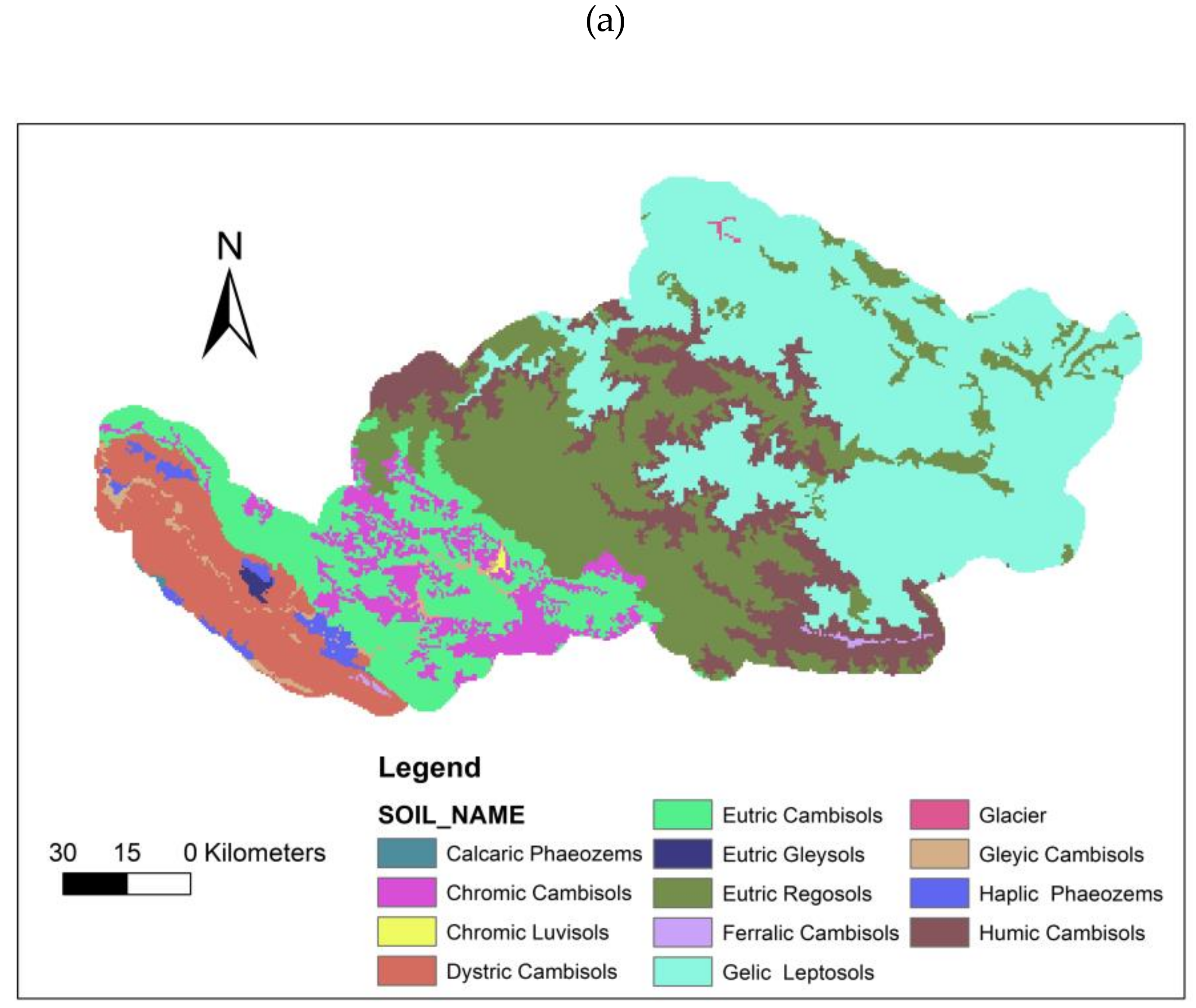
The whole basin is dominated by forests (34.7%), followed by snow cover/glaciers (15.9%), and then grasslands (15.8%); the built-up area covers the least portion (0.6%) (Figure 2). Gelic lepto soil (covers around 37% of the total basin area) is found in the northern mountainous areas, Eutric Rego soil in the middle mountainous region (covers around 22% of the total basin area), and Dystric Cambi soil (covers around 8% of the total basin area) in the southern flat areas. Snowmelt is the major source of water in this river during winter and spring. As the majority of the basin is very sparsely populated and contains little agricultural land (13.4%), a very small amount of water is used for irrigation. Therefore, this basin could serve as a very good water donor basin to the more populated and arable river basins around it. Currently, a project is under construction to transfer water from the Bheri River to the Babai River.
3. Materials and Methods
3.1. Data Collection
Meteorological and hydrological data from 1975 to 2013 for all stations (Figure 1 and Table 1) were acquired from the Department of Meteorology and Hydrology (DHM), Nepal. Only the data from one hydrological station were available, which is at the end of the Bheri River. Climate station density is also low because of the remoteness of the area and the large snow-covered areas that encompass it. Though rainfall data are measured in all of the five stations, maximum and minimum temperature measurements are carried out by only two stations: Surkhet and Dunai. Humidity, sunshine hours, and wind speed data are available only at the Surkhet station. All hydrological and meteorological data are available at a daily timescale.
Besides climate data, the Digital Elevation Model (DEM), soil, and land use data are the main inputs for the SWAT model. The Shuttle Radar Topography Mission (SRTM) DEM of 30 m resolution was used in this study. The land use map at 30 m resolution, and developed by the International Centre of Integrated Mountain Development (ICIMOD) [23] was used. Soil data and all the required information about soil were collected from the Soil and Terrain database (SOTER) for Nepal [24].
3.2. Representative Concentration Pathways Scenario Data and Bias Correction
Based on different radioactive forcing levels starting from 2.6 watt/m2 to 8.5 watt/m2 energy, four RCP scenarios, namely 2.6, 4.5, 6.5, and 8.5, were defined. The radioactive forcing level depends on the emission of carbon dioxide. In RCP 2.6, the emission is very low and is based on the assumption that human development will be more environment-friendly. While RCP 8.5 assumes a higher carbon dioxide emission—around 1370 ppm—by 2100 [1], RCP 4.5 and RCP 6.5 are in between these two. For this study, we chose two scenarios: RCP 4.5 and RCP 8.5. These two scenarios correspond to the Special Report on Emissions Scenarios (SRES) B1 and A1F1 in terms of temperature anomaly.
Initially, the GCMs for this study were selected from the literature review. More than ten GCMs that have already been used in the Hindukush Himalayan and other similar basins of Nepal were selected. The meteorological data of the baseline period (1975 to 2005) were compared to the data downscaled from those GCMs. After bias correction, we compared the results with the observed data, and the best-fitting three GCMs were selected. These three GCMs have been used extensively in climate projection studies in the Hindukush Himalayan and many basins in Nepal [25,26,27,28]. These GCMs have been produced by different international research centers, including (1) the Atmosphere and Ocean Research Institute (The University of Tokyo) (MIROC-ESM); (2) the Beijing Climate Center, China Meteorological Administration (BCC-CSM-1.1); and (3) the National Center for Atmospheric Research, USA (CCSM4). The details of the climate models used to project the climate change scenario in the study basin are shown in Table 2.
Due to its coarse resolution, GCM data needs to be downscaled to fit the required spatial resolution before using it in the SWAT model. Broadly, there are two types of downscaling methods: (1) dynamic downscaling wherein the Regional Climate Model (RCM) is placed inside the GCM, and (2) statistical downscaling, which is an empirical relationship developed between the GCM and the ground data for required stations and applied to the variables of interest.
In this study, the Linear Scale Factor (LSF) approach [29,30,31,32] under the statistical downscaling method was used. This method has been used for many basins [27]. In the LSF method, the monthly averages of the observed and simulated values of the constituent were used to compare the results before and after bias correction across all the stations. Different descriptive statistics such as R2, root mean square error (RMSE), standard deviation, and mean were used to check the suitability of the climate model. The values of the variables, with and without bias correction, were compared against the observed data. The enhancement of the parameter (increased R2, decreased RMSE, and closer to mean and standard deviation to the observed value) is one major criterion in selecting a GCM.
3.3. Model Setup, Calibration, and Validation
The SWAT model is a spatially semi-distributed, physically-based, continuous hydrological model developed by the United States Department of Agriculture (USDA) and Texas A&M University [33]. The model can be used to study future hydro-climatic changes by modifying the climate parameters based on future climate projections. In the SWAT model, a basin is divided into various sub-basins, which are then further divided into hydrologic response units (HRUs) that are comprised of unique land use, slope, and soil characteristics. The initial simulation of the hydrological cycle occurs at the HRU level, and excess discharge is then aggregated across the HRUs [34].
The ArcSWAT 2012 tool provided in the ArcGIS 10.1 system software was used to develop the SWAT model for the BRB. The major steps in SWAT modeling are basin delineation and river network extraction, HRU definition, climate station formation, parameter sensitivity analysis, calibration, and validation. As per the DEM and information from the digital stream network, the Bheri River Basin was delineated into 15 sub-basins. These sub-basins were further divided into 276 HRUs using the HRU definition threshold of 10% for each land use, soil, and slope. To account for orographic effects on both precipitation and temperature, SWAT allows up to 10 elevation bands to be defined in each sub basin. In this study, we generated 500 m elevation range band in each sub basin. TLAPS and PLAPS are also taking consideration during sensitivity analysis of the model. In addition, PLAPS is the sensitive parameter during model calibration. For computation of the potential evapotranspiration, the Penman-Monteith method was used, and the SWAT model was run from 1991 to 2006 for calibration and 2007 to 2013 for validation. The model warm up period was reserved for five years from 1986 to 1990.
The performance of the SWAT model can be evaluated using the coefficient of determination (R2), the Nash—Sutcliffe Efficiency index (NSE), and percent bias (PBIAS), which are calculated as follows [35]:
where is the ith observation for the parameter being evaluated; is the ith simulated value for the parameter being evaluated; is the mean of the observed data for the parameter being evaluated; and n is the total number of observations.
NSE indicates how well the plot of the observed versus the simulated data fits the 1:1 line, and its value can be between minus infinity to 1. An NSE value closer to 1 indicates a good result. PBIAS showed that the deviation of the evaluated parameter and the optimal value was zero percent. As per Moriasi et al. (2007) (Table 3), a model’s simulation performance can be considered satisfactory at an NSE greater than 0.5, PBIAS within ±25%, and R2 greater than 0.6.
Model parameter sensitivity analysis, calibration, and validation were performed with the SWAT-CUP tools (http://swat.tamu.edu/software/swat-cup/) by the sequential uncertainty-fitting algorithm (SUFI-2). It has the capacity to analyze many parameters during the model run. Initially, a large number of parameters were selected from literature. During calibration, the overall effect of each parameter used was ranked by using the global sensitivity function within SUFI-2, which also recommends the new parameter range for the next iteration so the model can be re-calibrated until the best parameter range is obtained. In SUFI-2, we can define the objective function to evaluate the quality of SWAT simulations. Mostly, the best fit in SUFI-2 is quantified by the R2 and Nash-Sutcliff (NS) coefficient between the observation data and the best simulation. In this study, we used 29 parameters [34] and ran 1000 simulations, and we identified the eleven most sensitive parameters guided by daily streamflow data.
4. Results
4.1. Performance of Bias Correction
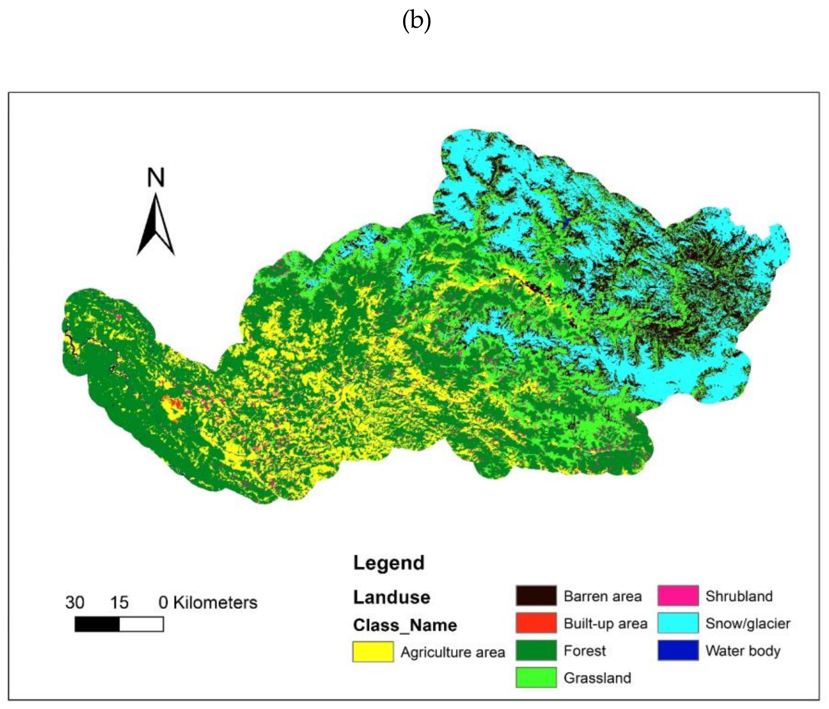
Table 4 presents the mean, R2, RMSE, and SD of the minimum and maximum temperature and rainfall of observed data, raw data (downloaded GCM data before bias correction), and corrected GCM data of all the stations of the BRB for the GCM model MIROC-ESM. After bias correction, the R2 for both the maximum and minimum temperature and rainfall showed an increase. Similarly, the mean and standard deviation of the bias corrected results were closer to the observed results. RMSE at all of the stations decreased after bias correction. The other two selected models also showed similar results under both the RCP 4.5 and RCP 8.5 scenarios. The monthly time series of the observed and simulated (from model MIROC-ESM) mean Tmax, Tmin and rainfall of the Dunai stations in the BRB are shown in Figure 3a–c. The mean monthly observed values of Tmax, Tmin, and rainfall for the baseline period were in close agreement with those from the bias corrected values. These results indicate that the downscaling technique significantly improved the quality of the GCM data. Overall, the results showed that downscaled data from these models could be reliably used for analyzing water availability in the future.
4.2. Parameter Sensitivity Analysis
The ranks of the 11 most sensitive parameters given by the SWAT-CUP from 29 input parameters [35] and 1000 simulations are presented in Table 5. The top three parameters were the base flow alpha factor (ALPHA_BF), initial SCS CN II value (CN2), and base flow alpha factor for bank storage (ALPHA_BNK).
4.3. Model Calibration and Validation
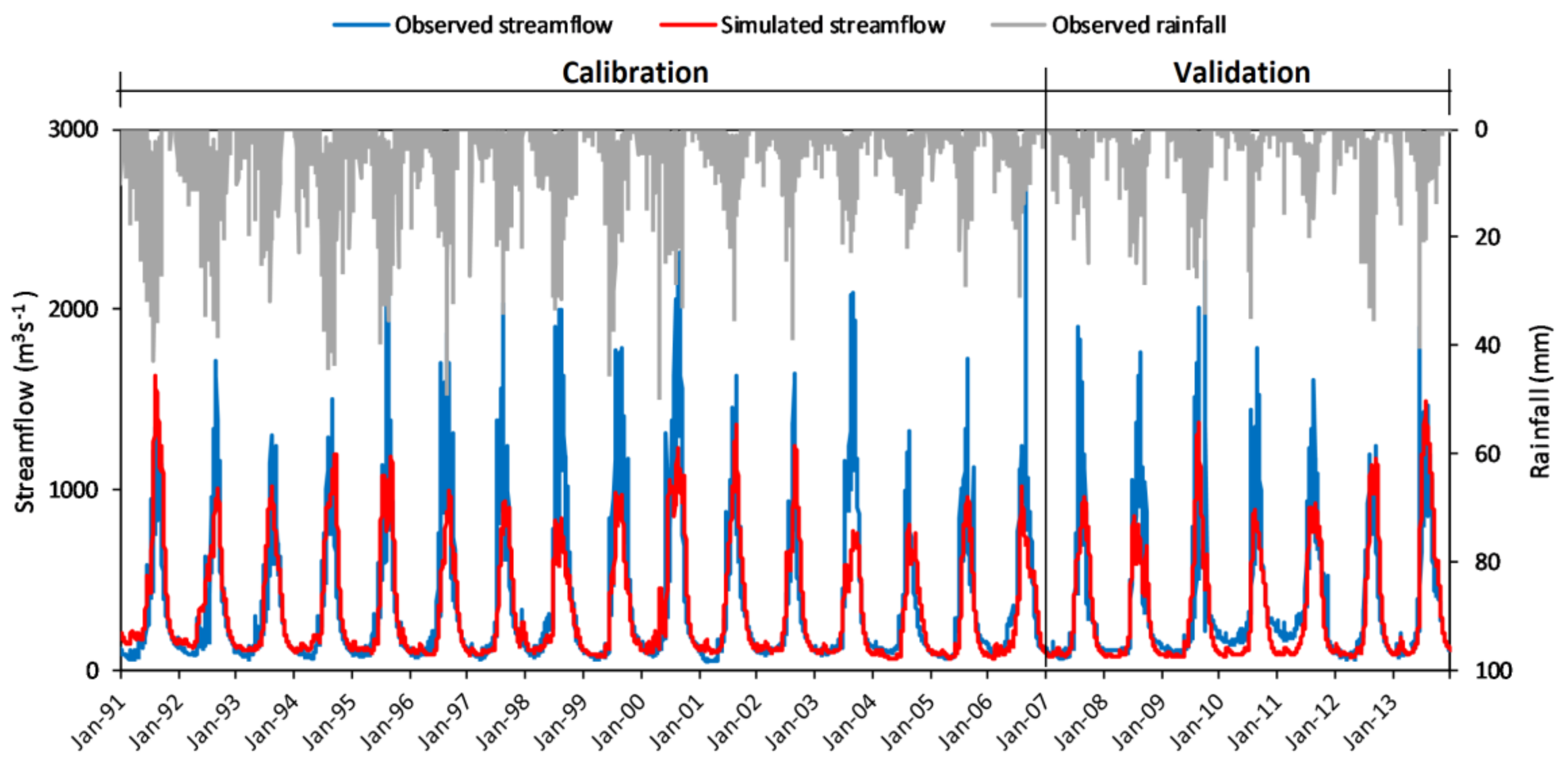
Figure 4 shows the calibration and validation results of the daily data along with rainfall. Calibration was carried out for the period from 1991–2006 (the period with comparatively less human intervention) and validation was carried out for the period from 2007–2013. The model’s warm- up period was reserved as 5 years, from 1986 to 1990. The same input parameters were used in the validation as per the calibration. Calibration and validation were carried out for daily datasets against the hydrological stations. The value of deterministic parameters such as NSE, R2, and PBIAS are shown in Table 6. Thus, based on the study of Moriasi et al. (2007) [35], the model performance fell under a good category. We acknowledge that during the calibration of the model, focus was given to baseflow matching. The peak flow was underestimated, and the model may not be used for flood estimation and forecasting. The model is therefore more useful for assessing the stream flow volume.
4.4. Future Temperature
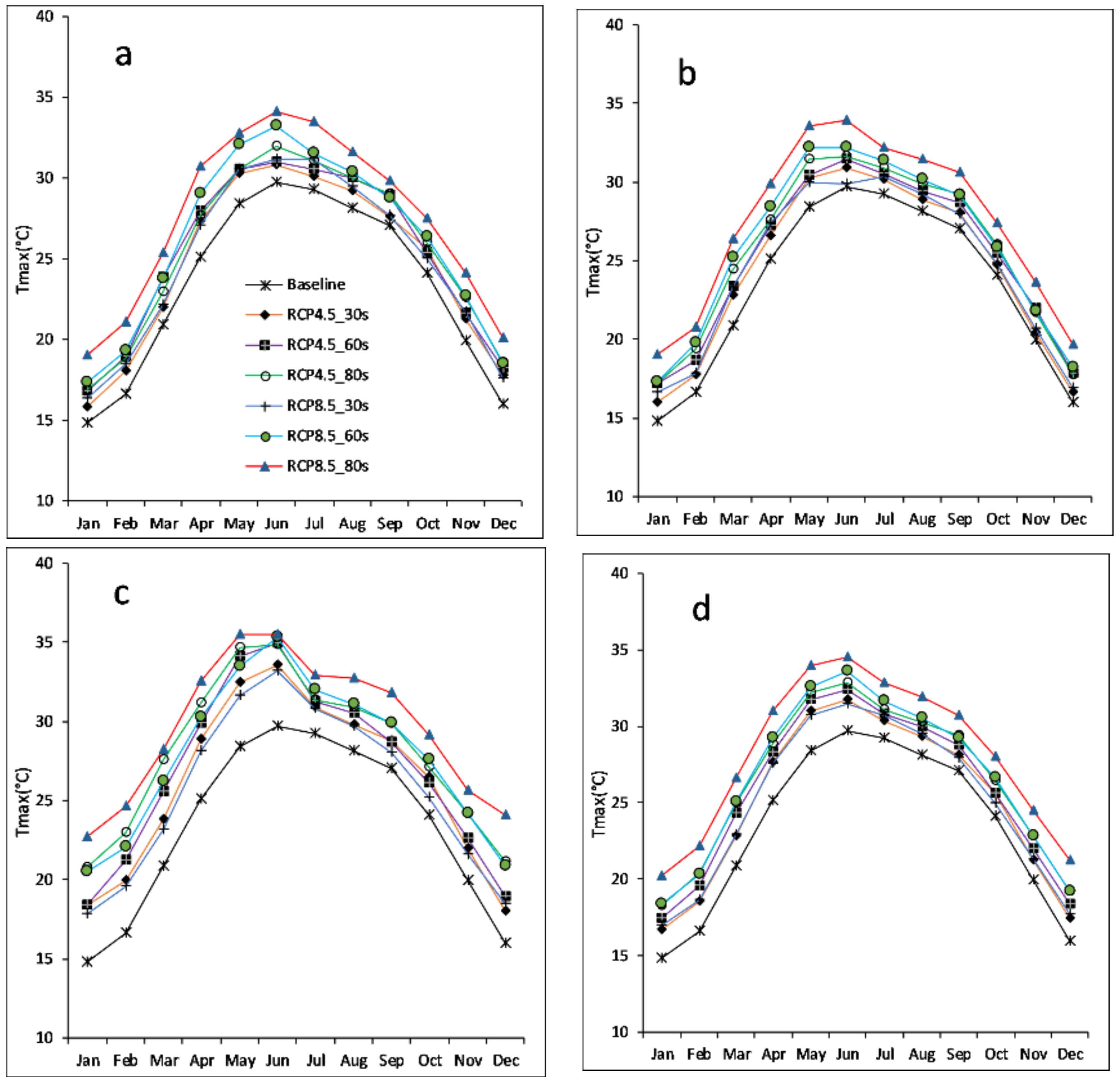
BCC-CSM1.1, CCSM4, and MIROC-ESM data were downloaded and bias corrected for all five stations of the Bheri River catchment. The combined information on a monthly basis is presented in Figure 5, Figure 6 and Figure 7 and on an annual basis in Table 7. Figure 5 shows the comparison between the projected monthly mean maximum temperature under RCP 4.5 and RCP 8.5 and the monthly mean maximum temperature during the baseline period (1975–2005). All the models projected a higher Tmax than that of the observed data of the baseline period (1975–2005). The increments range from 1 °C to 6 °C, depending on the scenario and the future period selected. Similar results have been found in previous studies carried out in this region [36,37]. In the higher mountainous regions of Nepal, the temperature increment is higher than in other parts of the country [3]. Furthermore, in this study, the temperature increase was greater at the Dunai station, which is located at a higher altitude than the Surkhet station. The Tmax increment was more in January to May than in the other months. The temperature could increase more under RCP 8.5 in the 80 s and less under RCP 4.5 during the 30 s period. MIROC-ESM predicted the highest amount of increment by up to around 7 °C, in the 80 s under RCP 8.5. BCC-CSM1 showed a moderate level of increment against the baseline data.
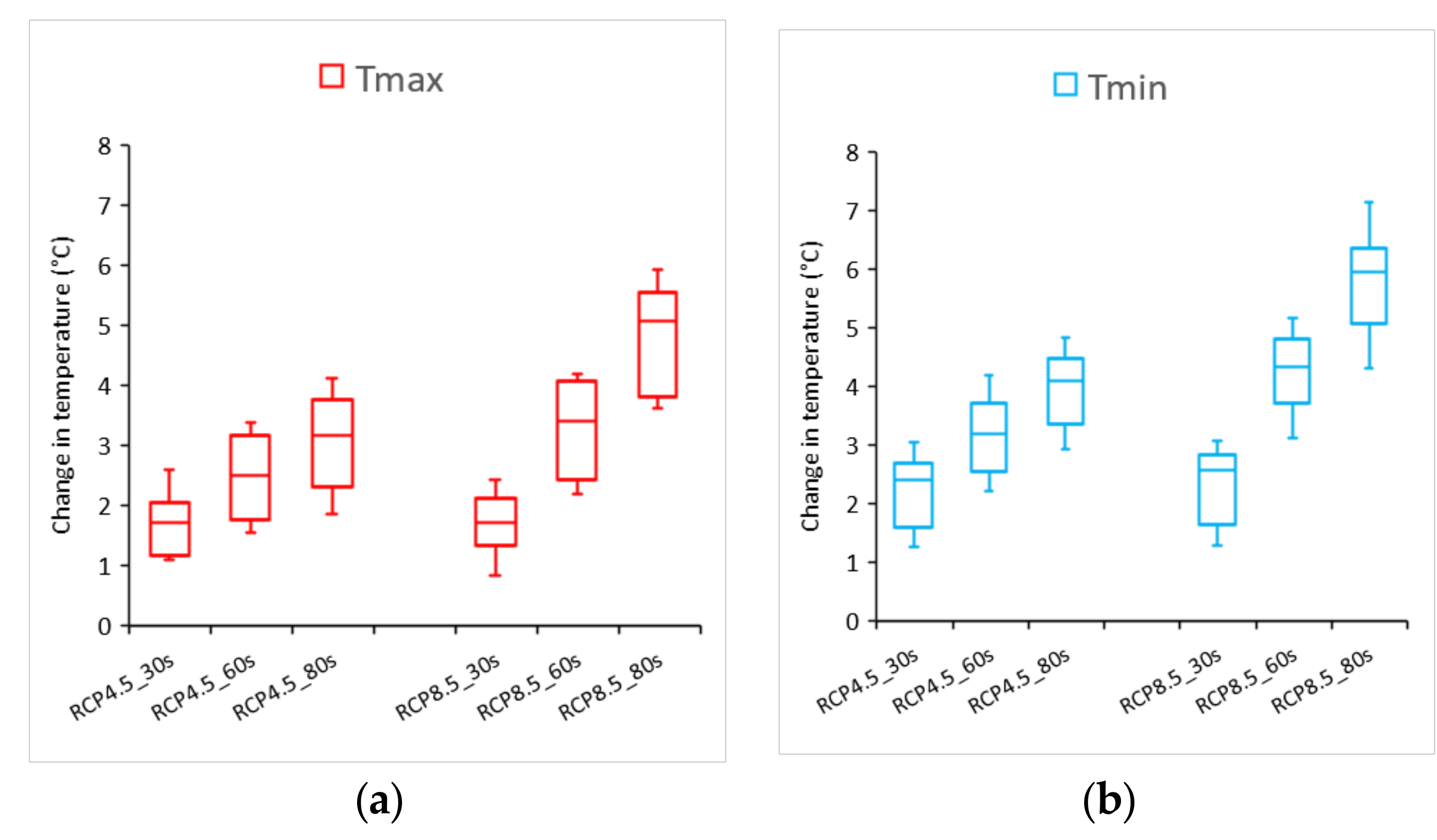
CCSM4 also estimated a mild level of increment in temperature across all months. Figure 6 shows the ensemble of change in the mean monthly maximum and minimum temperatures in the three future periods under the two RCP scenarios. The magnitude of variation of Tmin was higher than that of Tmax. The increment in Tmin during the study period was around 7.5 °C, whereas this value of Tmax was around 6 °C. Obviously, the increment was higher under RCP 8.5 than under RCP 4.5.
Table 7 presents the annual changes in Tmax and Tmin for the future for the three models relative to the observed data (of the period from 1975 to 2005) under both RCPs. The projected Tmax increased in all three periods, with the increase ranging from 1.3–4.1 °C for BCC-CSM1.1, 1.1–4.1 °C for CCSM4, and 2.3–7.1 °C for MIROC-ESM. The ensemble of the three GCMs projected that the temperature would increase between 1.7–3.1 °C under RCP 4.5, and 1.7–5.1 °C under RCP 8.5 for the selected future periods. Similarly, the ensemble of the three GCMs projected that Tmin would increase between 2.2–4 °C under RCP 4.5, and between 2.3–6.2 °C under RCP 8.5.
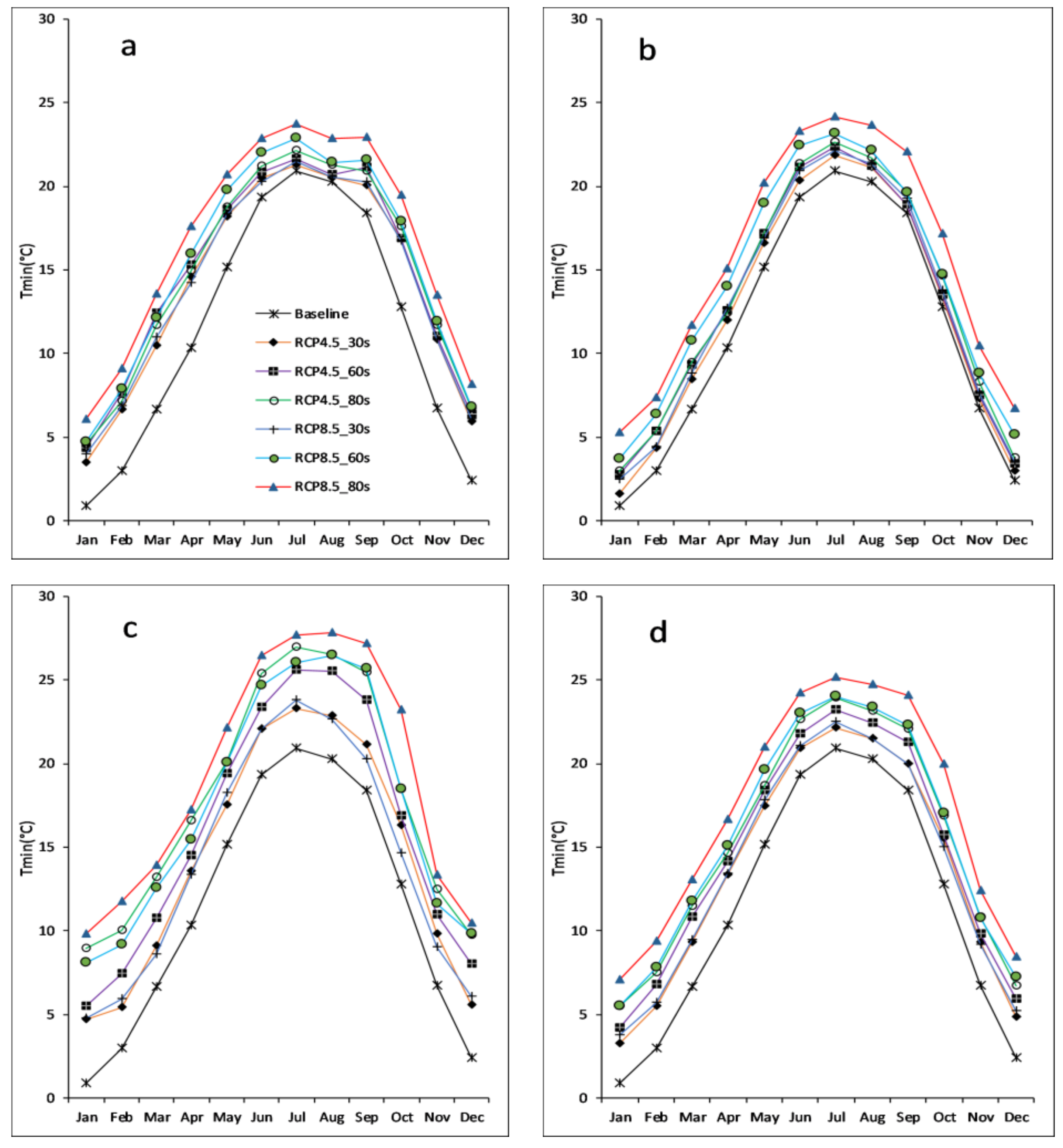
The downscaled results of the three GCMs showed that the future monthly minimum temperature would increase when compared to the baseline in all the months throughout the study period (Figure 7), but the trends were consistent with the observed data (that is, temperature rises from January to June and falls from July to December). The ensemble of the three GCMs showed that the increment varied from 4 °C to around 7 °C. All models predicted that the temperature might increase more under RCP 8.5 during the 80 s period, and less under RCP 4.5 during the 30 s period.
4.5. Future Rainfall
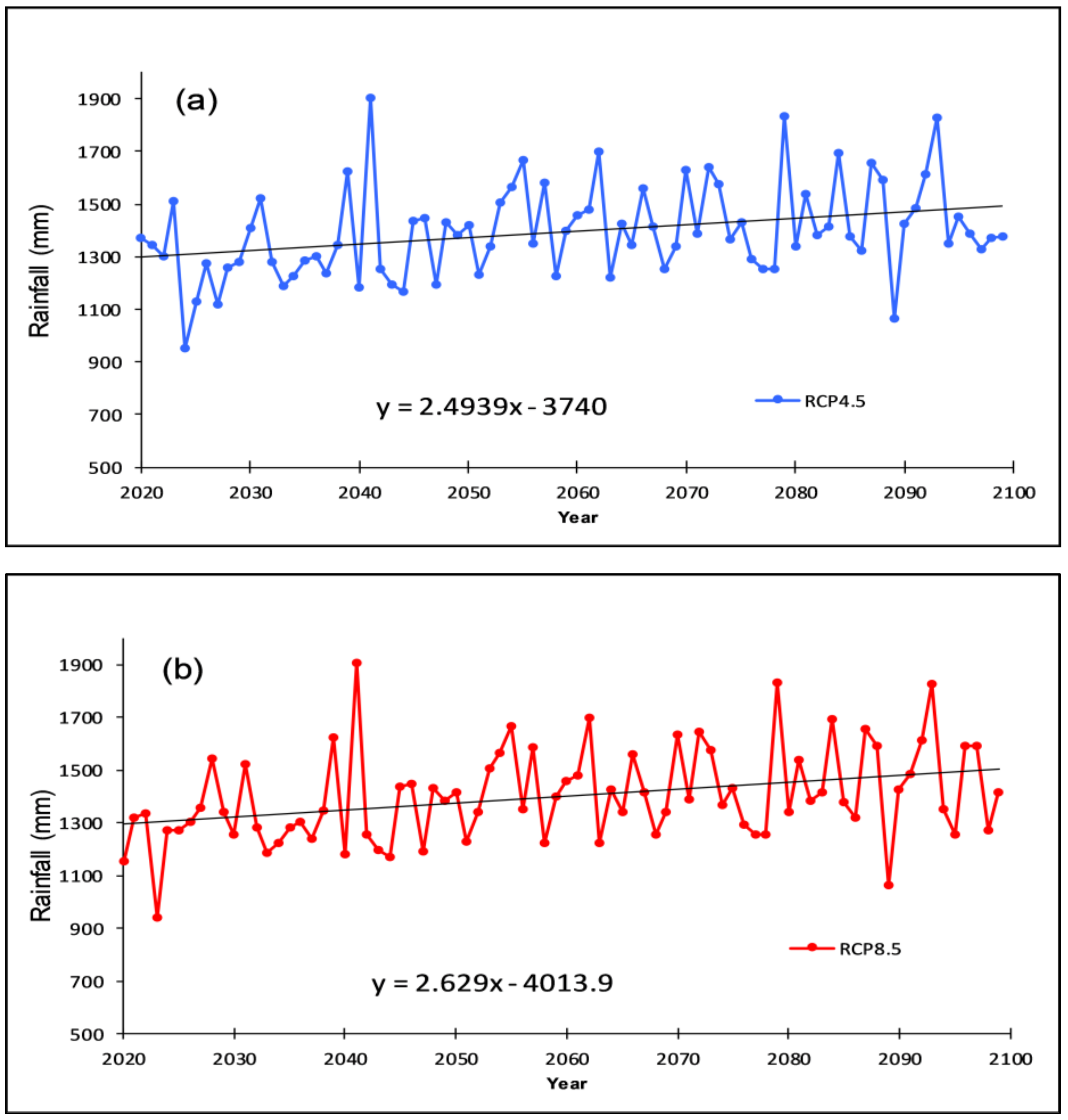
The rainfall projection under the two different scenarios for the three future time periods by the three GCMs and as aggregated by the Theisen polygon method is presented in Figure 8. A linear increasing trend was seen under both scenarios. The increment was higher under RCP 8.5 than under RCP 4.5. The modified Mann-Kendall test [38] showed that there was a significant trend in rainfall for both scenarios with p-values less than 0.01 at the 99% significance level. RCP 4.5 exhibited an increasing slope of 2.49 mm/year, while RCP 8.5 showed a slope of 2.63 mm/year with the Thiel-Sen slope estimator.
Table 8 presents the projected annual change in rainfall during the three future periods under the RCP 4.5 and RCP 8.5 scenarios. We observed an annual change in rainfall for individual GCMs and for the ensemble. All comparisons were made against the observed data of the baseline period (1975–2005). Under RCP 4.5, the annual rainfall was likely to increase by 6.8%, 7.4%, and 10.1% in the 30 s, 60 s, and 80 s, respectively when compared to the baseline period (1975–2005). Similarly, under RCP 8.5, this could increase by 7.3%, 10.7%, and 15.2% during the same time periods. Under RCP 4.5, the minimum (up to 6.4%) rainfall increment was obtained from MIROC-ESM and the maximum (14.2–16.6%) increment from CCSM4. Similarly, under RCP 8.5, the minimum (0–8.4%) and maximum (17.9–19.5 %) ranges were obtained from the same two GCMs. All the GCMs, except for MIROC-ESM (in the 30 s), showed that under RCP 8.5, rainfall could increase throughout the century, but under RCP 4.5, MIROC-ESM showed that rainfall could decrease in the 30 s by around 3%. The ensemble showed that rainfall would increase throughout the study period, and could increase from 6.8–10.1% under RCP 4.5, and 7.3–15.2% under RCP 8.5.
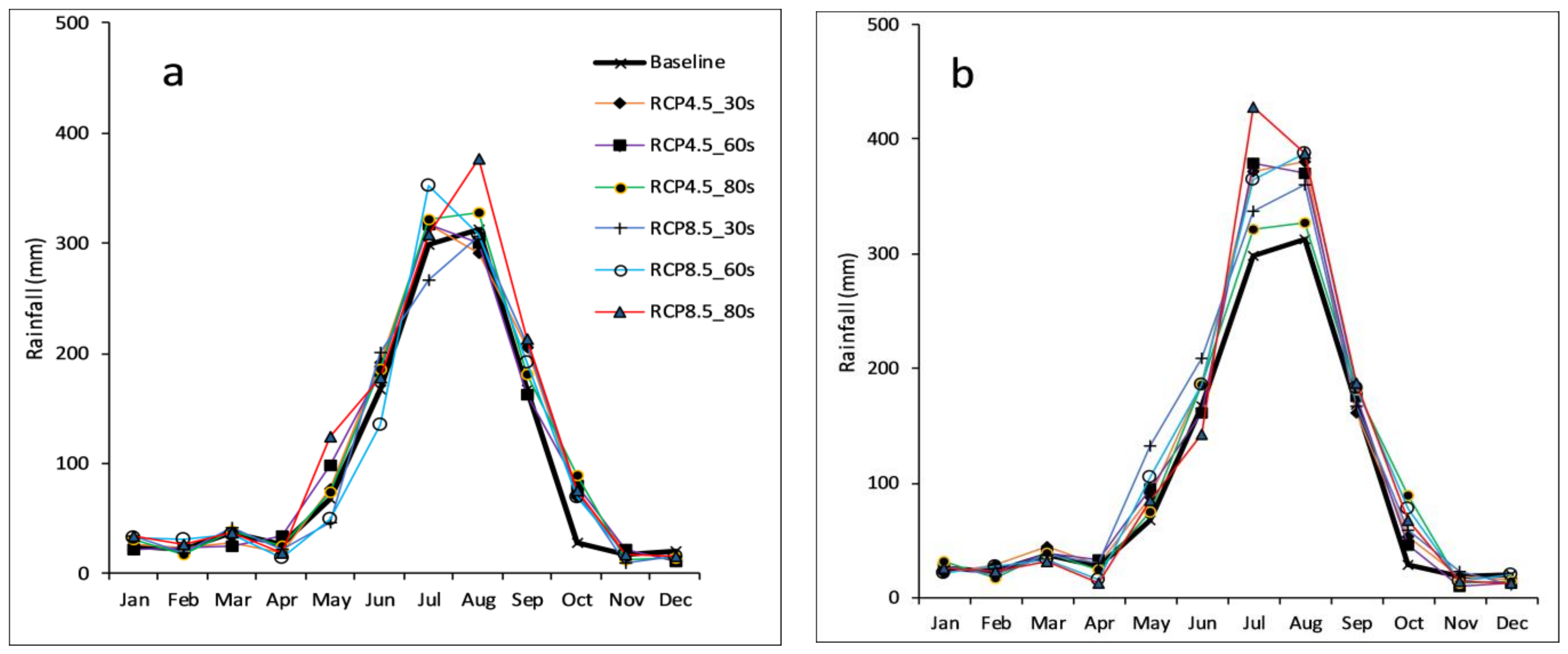
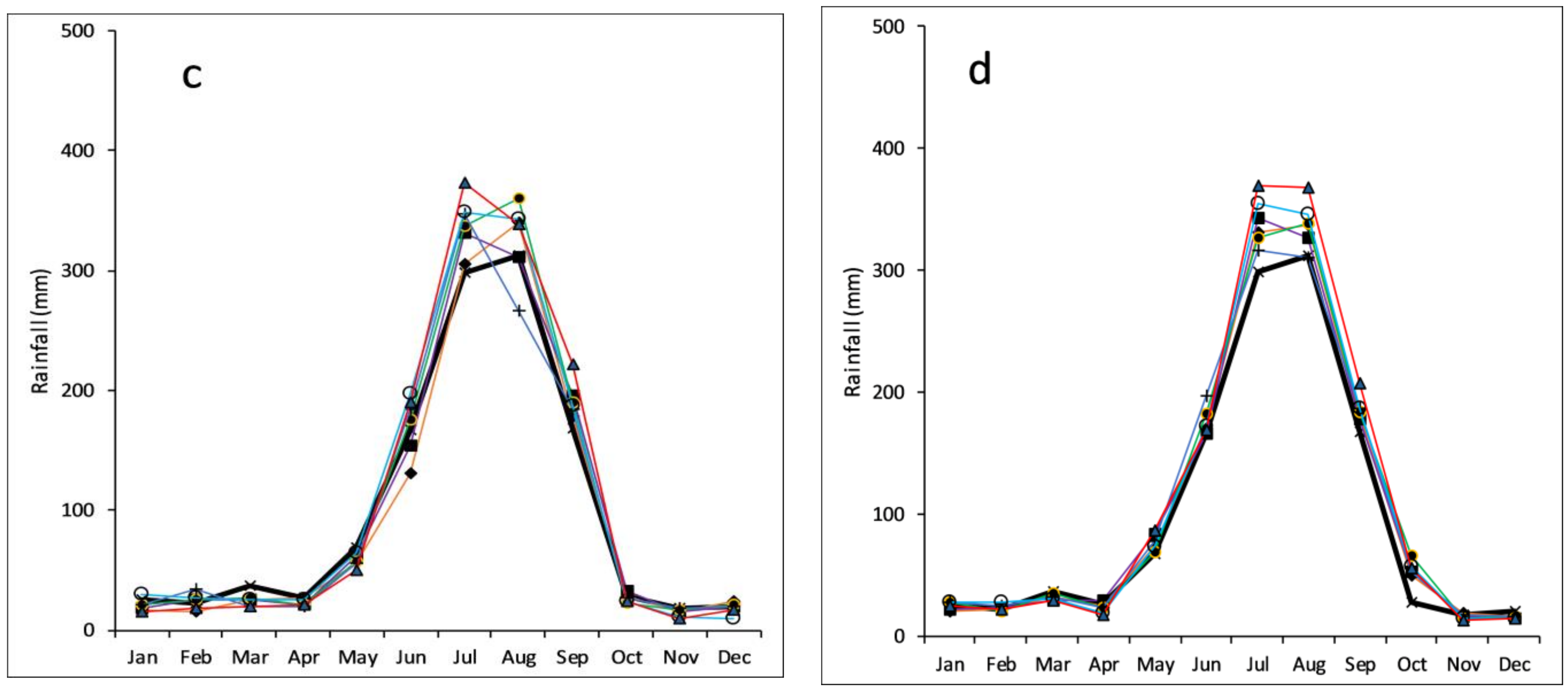
Figure 9 shows the monthly mean rainfall of the observed and projected data for the three future periods. The downscaled and bias corrected results of the future rainfall showed that the rainfall patterns would be similar to that of the observed period. A significant increase in rainfall in July and August under both RCPs was projected by all the models throughout the study periods. Among the three GCMs, CCSM4 predicted the highest amount of rainfall in the future.
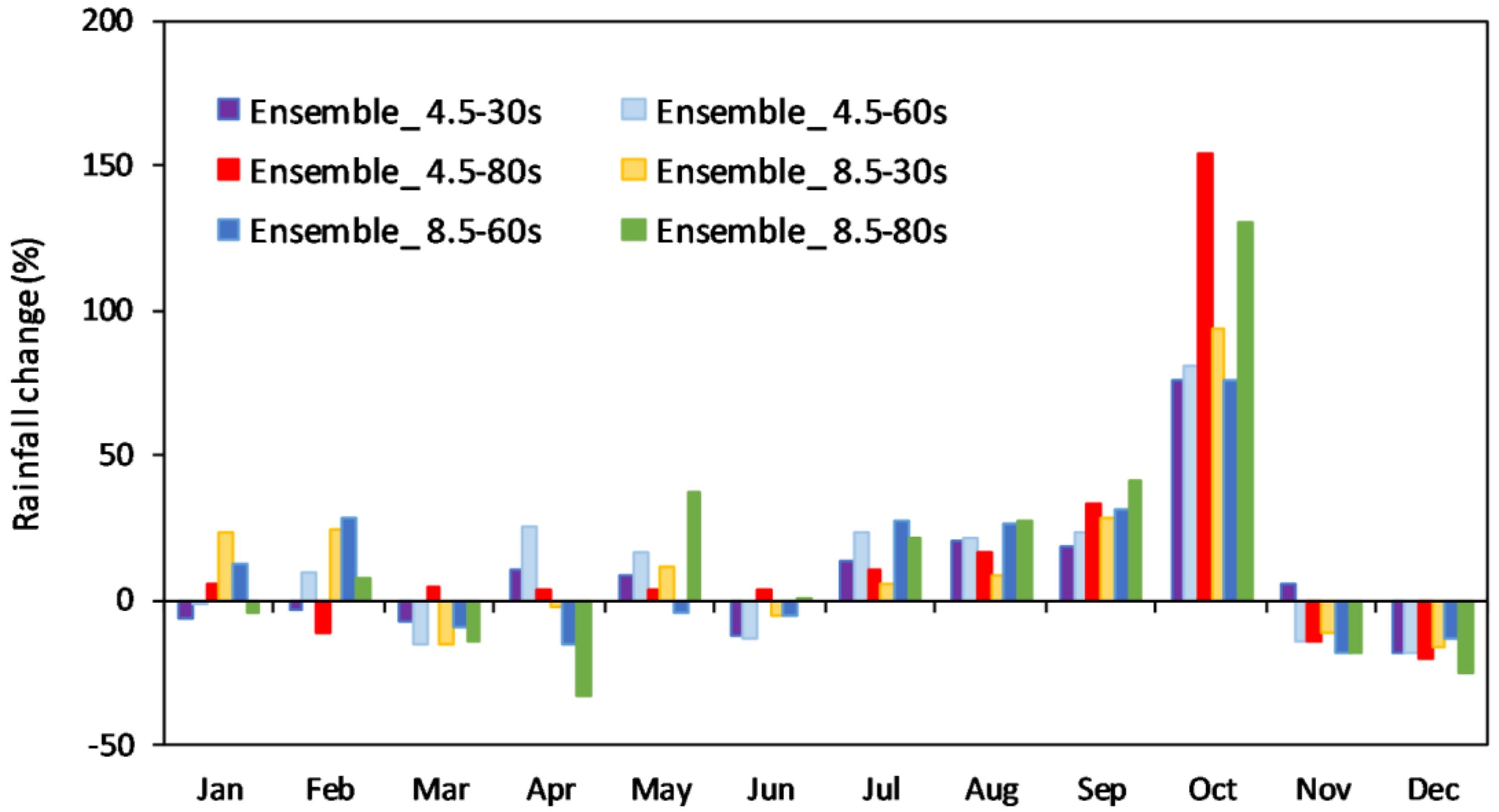
Figure 10 displays the changes (in percentage) in monthly rainfall in the ensemble of the three GCMs for the two scenarios during the three different future periods. It can be seen that monthly rainfall will increase dramatically, ranging from 76% to 154%, in October. Immediately after that, rainfall is likely to decrease in November and December by up to 24%. In November and December, the percentage decrease is 11% to 24%, and this corresponds to 2–6 mm of rainfall, which is negligible. Conversely, the 6–40% increase from July to September can mean up to 85 mm additional rainfall in these months. In June, the onset of the rainy season, rainfall could increase by up to 12%, which corresponds to about 65 mm of rainfall.
4.6. Future Streamflow
The streamflow obtained from the calibrated SWAT model with predicted temperature and rainfall under different climate change scenarios is shown in Table 8 and Figure 11 and Figure 12. All the comparisons were made against the observed streamflow of the baseline period (1975–2005). Table 8 shows that except for one instance of decreased flow in the 30 s, all the GCMs showed increased discharge in all three periods. BCCCSM1.1 showed an increasing trend in streamflow under both RCPs. Its range was around 5–9% under RCP 4.5 and around 2–17% under RCP 8.5. MIROC-ESM showed a decreasing trend in the 30 s, and an increasing trend in the 60 s and 80 s under both scenarios. CCSM4 showed flow increment to be about 16% in the 30 s under both scenarios, and about 5% under RCP 4.5 and 12% under RCP 8.5 in the 80 s. The ensemble of the three GCMs also predicted an increase in streamflow under both RCPs. Thus, it could be clearly concluded that the annual streamflow changes were compatible with the rainfall data.
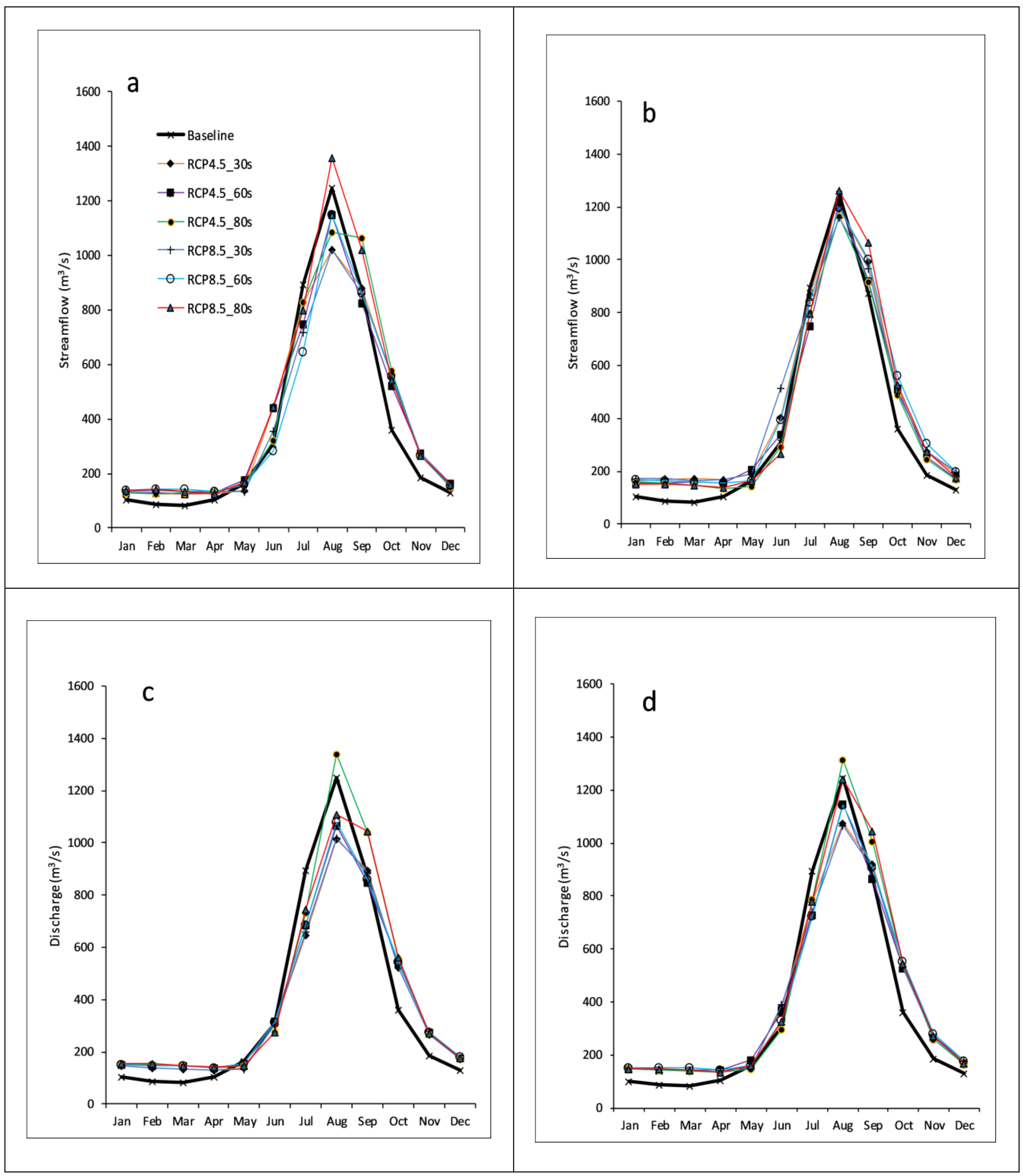
Figure 11 shows the monthly mean streamflow of different GCMs under different scenarios. In all the GCMs, the pattern of future monthly streamflow was similar to the baseline flow. The prediction of flow from June to August was highly variable with different GCMs. All the models predicted that the streamflow in the dry season would be higher than the baseline flow. All the models also showed that the peak would not shift and the flow pattern in the future was similar to the baseline pattern. According to the ensemble of the three models, the streamflow in a majority of the RCPs would increase from October to April, but decrease from June to August.
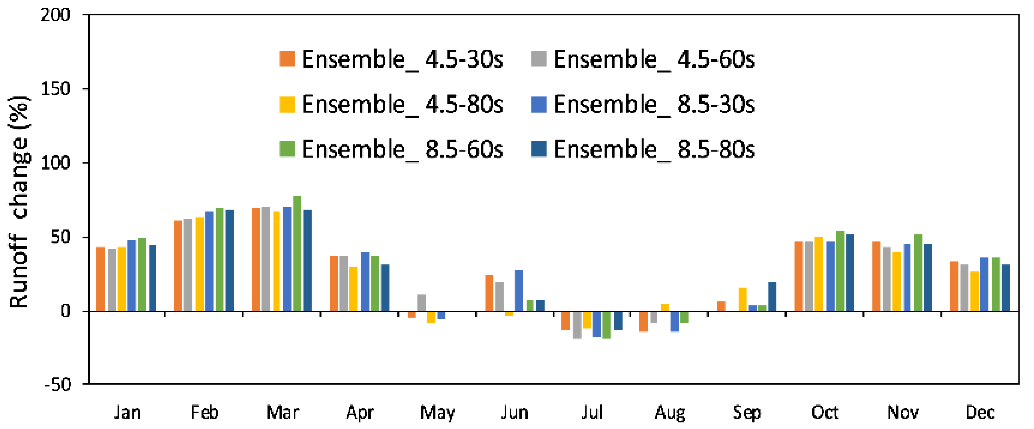
At the monthly analysis level, the ensemble of the three GCMs projected that the runoff would decrease in the months of July and August by up to 20%. The discharge would increase for all the remaining months. The monthly discharge variation showed remarkable results: it increased by around 40–70% from October to March, but decreased from April to June by around 30% and was less than the baseline flow in July and August (Figure 12). The maximum streamflow increment was projected for March (the increase will be by around 70%), followed by February (around 65%).
5. Discussion
The results obtained from the three GCMs under the two RCPs indicated that temperature was likely to increase across the basin across all months (Figure 5, Figure 6 and Figure 7). The increment was greater in the first five months of the year. The trend of projected temperature rise in this basin was similar to that of the historically observed data. The historical record showed an increase in average maximum temperature in the Surkhet station at the rate of 0.059 °C/year and an increase in minimum temperature by 0.023 °C/year over the past forty years (1975 to 2014). The ensemble of the three GCMs showed that under RCP 4.5, the changes in annual temperature will be +0.025 °C/year for maximum temperature and +0.033 °C/year for minimum temperature. As the temperature increasing rate was higher under higher emission scenarios, under RCP 8.5, the rate was +0.065 °C/year for maximum temperature, and +0.071 °C/year for minimum temperature, which was almost double in comparison to the increases in both the maximum and minimum temperature under RCP 4.5. The increasing rate was similar to the data gleaned in earlier studies of nearby basins that have similar topography [3,36,37]. Regarding rainfall (Figure 9 and Figure 10), the projection was different for different GCMs and RCPs. On an annual basis, negative to moderate (from −3% to 20%) change was projected for the near, mid, and far-future periods. Rainfall was almost equal to the baseline period from November to April, but was likely to increase from June to October.
When considering streamflow, the simulation results showed that the changes in mean annual rainfall and temperature will cause a significant change in annual surface runoff. The ensemble of the three GCMs’ runoff predicted a likely change from 6 to 12% in the study period. The greatest annual surface runoff increment (12.5%) was observed under the RCP 8.5 scenario in the 80 s. The ensemble surface runoff on a monthly basis in the basin was projected to increase by 68.4–70.1% in March, 67.6–68.1% in February, and 47.1–51.0% in October under the different scenarios. The largest increase under the RCP 4.5 scenario was also seen in the same three months, though the range of variation varied with different times of the year. Monthly variations in rainfall and streamflow were not consistent. From November to April, the average monthly rainfall in the baseline period was only between 18–36 mm, which means that there was none or very little contribution of rainfall to the streamflow during these months. The projected rainfall in these months fluctuated by around +/- 4 to 8 mm, which is about 20%. This change in rainfall did not contribute to streamflow, hence streamflow is solely contributed by natural spring water and snowmelt. As snow cover was assumed to stay unchanged and the temperature projected to increase by 1 to 6 °C from the 30 s to the 80 s, the snow melt rate will increase, which will consequently attribute to the increased flow in dry seasons. This result was quite consistent in all the GCMs considered and for all scenarios.
Since the Bheri River is considered to be a donor river in Western Nepal, the quantity of minimum flow in this river is vital. That forced us to match the base flow during the model’s calibration and validation (Figure 4). Consequently, the simulated flow obtained was around 20% lower than the observed flow in July and August during the calibration and validation of the model. This was reflected when we used the same model for predicting streamflow for the future and appeared to decrease even as it increased the rainfall in July and August. The simulation result of all scenarios (but one) showed that the future streamflow could decrease by up to 20% in July and August.
Considering the 250% crop intensity, the Babai River Basin (next to the BRB) is a water deficit basin from January to May [21,22]. The project initiated by the Department of Irrigation (DOI) to transfer water from the BRB to the Babai River was designed to facilitate year-round irrigation for all agricultural areas in the Babai River Basin. Since the predicted future discharge of the BRB could increase from 6 to 12% (when compared to the present flow) (see Table 8) under all scenarios, the water transfer project from the BRB to Babai appears to be sustainable.
There are a few uncertainties that still exist, which are mainly due to the limitations of this study. Uncertainties came from the GCMs chosen, the greenhouse gas emission scenarios under consideration, the hydrological model opted for, and the downscaling methods that were selected [39]. In the BRB, there are insufficient number of climatological stations and highest station located at 2058 m a.s.l. It shows the inability of rain gauge stations to capture the high intensity of local rainfall, which caused flood in the river. This was reflected during calibration and validation of the model, so that this model may not useful for flood estimation and forecasting. In addition, there is only one flow gauge, so we used the data from only one hydrological station for the calibration and validation of the model. That may not accurately reflect the spatial variation in sub-basin streamflow [40]. We recommend the Department of Hydrology and Meteorology Nepal to establish telemetry-based station in the upper zone of the basin that would be highly useful for future study. The land use of the basin was also kept unchanged during the whole simulation period, which may not happen in reality. This is especially true for land use, which has a substantial effect on streamflow [41]. The model predicted that water availability in the Bheri River was not likely to decrease in the future (see Table 8 and Figure 11), and by considering the water demand in the BRB in the present scenario, the Bheri River can be thought of as an ideal donor river. Due to the impact of climate change, the demands for water in the BRB itself may vary in the future, so more studies related to the impact of climate change as far as water demand is concerned need to be carried out in this basin.
6. Conclusions
In this study, we analyzed the impacts of climate change on temperature, rainfall, and streamflow in the BRB. Future climate change in the basin was projected using three GCMs under RCPs 4.5 and 8.5 for the periods of 2020–2044, 2045–2069, and 2070–2099. Future Tmax, Tmin, and rainfall were projected using the SDSM of the data from the three GCMs under different scenarios. These data were then used as input for the calibrated SWAT model to obtain future discharge. Finally, the effects of climate change on streamflow regimes under those GCMs and scenarios were analyzed and compared to the baseline data. The most remarkable findings of this study can be summarized as follows:
- In daily calibration, primarily focused on low flow, the SWAT model performed satisfactory performance in the BRB. The indices (NSE and R2 greater than 0.7 for both calibration and validation and PBIAS −4.4% for calibration and −8.9% for validation) showed a satisfactory performance at the daily timescale. Considering the data deficit environment, the calibrated model represented the hydrological processes of the basin and acceptably predicted future streamflows in the BRB.
- All models showed that future temperature (Tmax and Tmin) could increase throughout the century. The increment was higher from January to May than from June to December. Temperature showed an increasing trend, and the ensemble of the three GCMs showed the rising trend of minimum and maximum temperature to be 0.033 °C/year and 0.025 °C/year for RCP 4.5, and 0.071 °C/year and 0.065 °C/year for RCP 8.5, respectively. Similarly, the downscaled results showed that rainfall would also increase in the future. RCP 4.5 exhibited an increasing trend of 2.49 mm/year, while RCP 8.5 showed an increase of 2.63 mm/year. However, there were some differences contingent upon different GCMs and scenarios.
- The ensemble of the three GCMs showed an annual streamflow rise by 6.2–7.3% under RCP 4.5, and 6.0–12.5% under RCP 8.5. However, the prediction was different for every GCM and scenario. CCSM4 predicted the highest rate of increase in annual flow (16.9% under RCP 8.5 in the 60 s). On a monthly scale, all the models under all scenarios (except RCP 4.5 in the 80 s and RCP 8.5 in the 80 s) predicted that the streamflows would decrease in July and August, relative to the baseline flow. The average monthly flow in spring and winter would also increase significantly. The ensemble’s results showed that the monthly increment can go up to 70% in February and March. The hydrological processes of streamflows for each GCM presented similar trends when compared to the baseline. This analysis suggests that the Bheri River could be a good donor river to the nearby water deficit basin.
Acknowledgements
We would like to acknowledge the Department of Hydrology and Meteorology Nepal, for providing the data. We also acknowledge the Government of Japan and the Asian Institute of Technology, Thailand, for providing the scholarship for the first author.
Author Contributions
All authors contributed to this study. Mishra and Babel conceived and designed the data and experiments. Mishra, Nakamura, and Babel developed the methodology and performed experiments. Mishra, Sarawut, and Ochi contributed to the analysis of the results and interpretation. Mishra wrote the original draft and all authors contributed in reviewing and editing the manuscript.
Conflicts of Interest
The authors declare no conflict of interest.
References
- Intergovernmental Panel on Climate Change (IPCC). AR5—Summary for Policymakers. In Climate Change 2013: The Physical Science Basis; Contribution of Working Group I to the Fifth Assessment Report of the Intergovernmental Panel on Climate Change; Cambridge University Press: Cambridge, UK; New York, NY, USA, 2013; p. 78. [Google Scholar]
- Maskey, S.; Uhlenbrook, S.; Ojha, S. An analysis of snow cover changes in the Himalayan region using MODIS snow products and in-situ temperature data. Clim. Chang. 2011, 108, 391–400. [Google Scholar] [CrossRef]
- Shrestha, A.B.; Wake, C.P.; Mayewski, P.A.; Dibb, J.E. Maximum temperature trends in the Himalaya and its vicinity: An analysis based on temperature records from Nepal for the period 1971-94. J. Clim. 1999, 12, 2775–2786. [Google Scholar] [CrossRef]
- Hu, Y.; Maskey, S.; Uhlenbrook, S. Trends in temperature and rainfall extremes in the Yellow River source region, China. Clim. Chang. 2012, 110, 403–429. [Google Scholar] [CrossRef]
- Bartlett, R.; Bharati, L.; Pant, D.; Hpsterman, H.; McCprnick, P. Climate Change Impacts and Adaptation in Nepal; IWMI Working Paper 139; International Water Management Institute (IWMI): Colombo, Sri Lanka, 2010. [Google Scholar]
- Immerzeel, W.W.; van Beek, L.P.H.; Konz, M.; Shrestha, A.B.; Bierkens, M.F.P. Hydrological response to climate change in a glacierized catchment in the Himalayas. Clim. Chang. 2012, 110, 721–736. [Google Scholar] [CrossRef] [PubMed]
- Trenberth, K.E. Changes in precipitation with climate change. Clim. Res. 2011, 47, 123–138. [Google Scholar] [CrossRef]
- Gonzalez, P.; Neilson, R.P.; Lenihan, J.M.; Drapek, R.J. Global patterns in the vulnerability of ecosystems to vegetation shifts due to climate change. Glob. Ecol. Biogeogr. 2010, 19, 755–768. [Google Scholar] [CrossRef]
- Pierce, D.W.; Barnett, T.P.; Santer, B.D.; Gleckler, P.J. Selecting global climate models for regional climate change studies. Proc. Natl. Acad. Sci. USA 2009, 106, 8441–8446. [Google Scholar] [CrossRef] [PubMed]
- Tan, M.L.; Ficklin, D.L.; Ibrahim, A.; Yusop, Z. Impacts and uncertainties of climate change on streamflow of the Johor River Basin, Malaysia using a CMIP5 General Circulation Model ensemble. J. Water Clim. Chang. 2014, 5, 676–695. [Google Scholar] [CrossRef]
- Sellami, H.; Benabdallah, S.; la Jeunesse, I.; Vanclooster, M. Quantifying hydrological responses of small Mediterranean catchments under climate change projections. Sci. Total Environ. 2016, 543, 924–936. [Google Scholar] [CrossRef] [PubMed]
- Zhang, Y.; You, Q.; Chen, C.; Ge, J. Impacts of climate change on streamflows under RCP scenarios: A case study in Xin River Basin, China. Atmos. Res. 2016, 178–179, 521–534. [Google Scholar] [CrossRef]
- Meinshausen, M.; Smith, S.J.; Calvin, K.; Daniel, J.S.; Kainuma, M.L.T. The RCP greenhouse gas concentrations and their extensions from 1765 to 2300. Clim. Chang. 2011, 109, 213–241. [Google Scholar] [CrossRef]
- van Vuuren, D.P.; Edmonds, J.; Kainuma, M.; Riahi, K.; Thomson, A.; Hibbard, K.; Hurtt, G.C.; Kram, T.; Krey, V.; Lamarque, J.; et al. The representative concentration pathways: An overview. Clim. Chang. 2011, 109, 5–31. [Google Scholar] [CrossRef]
- Tan, M.L.; Ibrahim, A.L.; Yusop, Z.; Chua, V.P.; Chan, N.W. Climate change impacts under CMIP5 RCP scenarios on water resources of the Kelantan River Basin, Malaysia. Atmos. Res. 2017, 189, 1–10. [Google Scholar] [CrossRef]
- Agarwal, A.; Babel, M.S.; Maskey, S. Estimating the Impacts and Uncertainty of Climate Change on the Hydrology and Water Resources of the Koshi River Basin. In Managing Water Resources under Climate Uncertainty; Springer: Berlin, Germany, 2015. [Google Scholar]
- Wu, K.; Johnston, C.A. Hydrologic response to climatic variability in a Great Lakes Watershed: A case study with the SWAT model. J. Hydrol. 2007, 337, 187–199. [Google Scholar] [CrossRef]
- Palazzoli, I.; Maskey, S.; Uhlenbrook, S.; Nana, E.; Bocchiola, D. Impact of prospective climate change on water resources and crop yields in the Indrawati basin, Nepal. Agric. Syst. 2015, 133, 143–157. [Google Scholar] [CrossRef]
- Gurung, P.; Bharati, L.; Karki, S. Application of the SWAT Model to assess climate change impacts on water balances and crop yields in the West Seti River Basin. In Proceedings of the 2013 International SWAT Conference, Toulouse, France, 17–19 July 2013; pp. 175–191. [Google Scholar]
- Dahal, V.; Shakya, N.M.; Bhattarai, R. Estimating the Impact of Climate Change on Water Availability in Bagmati Basin, Nepal. Environ. Process. 2016, 3, 1–17. [Google Scholar] [CrossRef]
- Water and Energy Commission Secretariat. Water Resources Strategy; Water and Energy Commission Secretariat: Kathmandu, Nepal, 2002; pp. 1–31. [Google Scholar]
- Adhikari, B.; Verhoeven, R.; Troch, P. Fair and sustainable irrigation water management in the Babai basin, Nepal. Water Sci. Technol. 2009, 59, 1505–1513. [Google Scholar] [CrossRef] [PubMed]
- Uddin, K.; Shrestha, H.L.; Murthy, M.S.; Bajracharya, B.; Shrestha, B.; Gilani, H.; Pradhan, S.; Dangol, B. Development of 2010 national land cover database for the Nepal. J. Environ. Manag. 2015, 148, 82–90. [Google Scholar] [CrossRef] [PubMed]
- Soil and Terrain Database (SOTER) for Nepal. Available online: http://www.isric.org/documents/document-type/isric-report-200901-soil-and-terrain-database-nepal-11-million (accessed on 04 March 2017).
- Mishra, V.; Kumar, D.; Ganguly, A.R.; Sanjay, J.; Mujumdar, M.; Krishnan, R.; Shah, R.D. Reliability of regional and global climate models to simulate precipitation extremes over India. J. Geophys. Res. Atmos. 2014, 119, 9301–9323. [Google Scholar] [CrossRef]
- Das, L.; Dutta, M.; Mezghani, A.; Benestad, R.E. Use of observed temperature statistics in ranking CMIP5 model performance over the Western Himalayan Region of India. Int. J. Climatol. 2017. [CrossRef]
- Shrestha, S.; Shrestha, M.; Babel, M.S. Modelling the potential impacts of climate change on hydrology and water resources in the Indrawati River Basin, Nepal. Environ. Earth Sci. 2016, 75, 280. [Google Scholar] [CrossRef]
- Mishra, B.; Tripathi, N.K.; Babel, M.S. An artificial neural network-based snow covers predictive modeling in the higher Himalayas. J. Mt. Sci. 2014, 11, 825–837. [Google Scholar]
- Teutschbein, C.; Seibert, J. Bias correction of regional climate model simulations for hydrological climate-change impact studies: Review and evaluation of different methods. J. Hydrol. 2012, 456–457, 12–29. [Google Scholar] [CrossRef]
- Ines, A.V.M.; Hansen, J.W. Bias correction of daily GCM rainfall for crop simulation studies. Agric. For. Meteorol. 2006, 138, 44–53. [Google Scholar] [CrossRef]
- Ouyang, F.; Zhu, Y.; Fu, G.; Lü, H.; Zhang, A.; Yu, Z.; Chen, X. Impacts of climate change under CMIP5 RCP scenarios on streamflow in the Huangnizhuang catchment. Stoch. Environ. Res. Risk Assess. 2015, 29, 1781–1795. [Google Scholar] [CrossRef]
- Basheer, A.K.; Lu, H.; Omer, A.; Ali, A.B.; Abdelgader, A.M.S. Impacts of climate change under CMIP5 RCP scenarios on the streamflow in the Dinder River and ecosystem habitats in Dinder National Park, Sudan. Hydrol. Earth Syst. Sci. 2016, 20, 1331–1353. [Google Scholar] [CrossRef]
- Arnold, J.G.; Srinivasan, R.; Muttiah, R.S.; Williams, J.R. Large area hydrologic modeling and assesment Part I: Model development. JAWRA J. Am. Water Resour. Assoc. 1998, 34, 73–89. [Google Scholar] [CrossRef]
- Arnold, J.G.; Moriasi, D.N.; Gassman, P.W.; Abbaspour, K.C.; White, M.J.; Srinivasan, R.; Santhi, C.; Harmel, R.D.; van Griensven, A.; van Liew, M.W.; et al. Swat: Model Use, Calibration, and Validation. ASABE 2012, 55, 1491–1508. [Google Scholar] [CrossRef]
- Moriasi, D.N.; Arnold, J.G.; van Liew, M.W.; Bingner, R.L.; Harmel, R.D.; Veith, T.L. Model Evaluation Guidelines for Systematic Quantification of Accuracy in Watershed Simulations. Trans. ASABE 2007, 50, 885–900. [Google Scholar] [CrossRef]
- Nepal, S. Impacts of climate change on the hydrological regime of the Koshi river basin in the Himalayan region. J. Hydro-Environ. Res. 2016, 10, 76–89. [Google Scholar] [CrossRef]
- Li, H.; Xu, C.Y.; Beldring, S.; Tallaksen, L.M.; Jain, S.K. Water resources under climate change in himalayan basins. Water Resour. Manag. 2016, 30, 843–859. [Google Scholar] [CrossRef]
- Mishra, B.; Babel, M.S.; Tripathi, N.K. Analysis of climatic variability and snow cover in the Kaligandaki River Basin, Himalaya, Nepal. Theor. Appl. Climatol. 2014, 116, 681–694. [Google Scholar] [CrossRef]
- Bosshard, T.; Carambia, M.; Goergen, K.; Kotlarski, S.; Krahe, P.; Zappa, M.; Schär, C. Quantifying uncertainty sources in an ensemble of hydrological climate-impact projections. Water Resour. Res. 2013, 49, 1523–1536. [Google Scholar] [CrossRef]
- Musau, J.; Sang, J.; Gathenya, J.; Luedeling, E. Hydrological responses to climate change in Mt. Elgon watersheds. J. Hydrol. Reg. Stud. 2015, 3, 233–246. [Google Scholar] [CrossRef]
- Zhou, J.; He, D.; Xie, Y.; Liu, Y.; Yang, Y.; Sheng, H.; Guo, H.; Zhao, L.; Zou, R. Integrated SWAT model and statistical downscaling for estimating streamflow response to climate change in the Lake Dianchi watershed, China. Stoch. Environ. Res. Risk Assess. 2015, 29, 1193–1210. [Google Scholar] [CrossRef]
Figure 1.
Location of the Bheri River Basin with its hydrological and meteorological stations.

Figure 2.
(a) Soil types (top) and (b) Land use (bottom) maps of the Bheri River Basin.


Figure 3.
Observed and bias corrected value of (a) Tmax; (b) Tmin; and (c) rainfall at the Dunai Station of Bheri River Basin.
Figure 3.
Observed and bias corrected value of (a) Tmax; (b) Tmin; and (c) rainfall at the Dunai Station of Bheri River Basin.

Figure 4.
Comparison of rainfall, observed, and simulated streamflow data at a daily timescale.

Figure 5.
Comparison of monthly mean Tmax between observed (1975–2005) and projected climate during the three future periods. (a) BCC-CSM1.1; (b) CCSM4; (c) MIROC-ESM; and (d) Ensemble.
Figure 5.
Comparison of monthly mean Tmax between observed (1975–2005) and projected climate during the three future periods. (a) BCC-CSM1.1; (b) CCSM4; (c) MIROC-ESM; and (d) Ensemble.

Figure 6.
Absolute changes in monthly mean (a) maximum and (b) minimum temperatures in the Bheri River Basin under the two RCP scenarios for the 30 s, 60 s, and 80 s periods, relative to the baseline (1975–2005).
Figure 6.
Absolute changes in monthly mean (a) maximum and (b) minimum temperatures in the Bheri River Basin under the two RCP scenarios for the 30 s, 60 s, and 80 s periods, relative to the baseline (1975–2005).

Figure 7.
Comparison of monthly mean Tmin between the observed (1975–2005) and projected climate during the three future periods. (a) BCC-CSM1.1; (b) CCSM4; (c) MIROC-ESM; and (d) Ensemble.
Figure 7.
Comparison of monthly mean Tmin between the observed (1975–2005) and projected climate during the three future periods. (a) BCC-CSM1.1; (b) CCSM4; (c) MIROC-ESM; and (d) Ensemble.

Figure 8.
Total annual future rainfall and trends for: (a) RCP 4.5 (top); and (b) RCP 8.5 (bottom) in the BRB.
Figure 8.
Total annual future rainfall and trends for: (a) RCP 4.5 (top); and (b) RCP 8.5 (bottom) in the BRB.

Figure 9.
Comparison of monthly rainfall between observed (1975–2005) and projected climate in the three future periods. (a) BCC-CSM1.1; (b) CCSM4; (c) MIROC-ESM; and (d) Ensemble.
Figure 9.
Comparison of monthly rainfall between observed (1975–2005) and projected climate in the three future periods. (a) BCC-CSM1.1; (b) CCSM4; (c) MIROC-ESM; and (d) Ensemble.


Figure 10.
Relative changes in monthly rainfall in the BRB under the RCP scenarios for the 30 s, 60 s, and 80 s periods, with respect to the observed rainfall (1975–2005).
Figure 10.
Relative changes in monthly rainfall in the BRB under the RCP scenarios for the 30 s, 60 s, and 80 s periods, with respect to the observed rainfall (1975–2005).

Figure 11.
Comparison of the monthly mean streamflow between the observed (1975–2005) and the projected periods. (a) BCC-CSM1.1; (b) CCSM4; (c) MIROC-ESM; and (d) Ensemble.
Figure 11.
Comparison of the monthly mean streamflow between the observed (1975–2005) and the projected periods. (a) BCC-CSM1.1; (b) CCSM4; (c) MIROC-ESM; and (d) Ensemble.

Figure 12.
Relative changes in the monthly mean streamflow in the BRB under the RCP scenarios during the 30 s, 60 s, and 80 s periods against the observed period (1975–2005).
Figure 12.
Relative changes in the monthly mean streamflow in the BRB under the RCP scenarios during the 30 s, 60 s, and 80 s periods against the observed period (1975–2005).


Table 1.
Basic information about hydro-climatic station in the Bheri river basin.
| SR | Station Meteorological | Lat (°N) | Long (°N) | Altitude (m ASL) | Period (Year) | Rainfall Annual (mm) | TX Mean (°C) | TN Mean (°C) |
| 1 | Dunai | 28.933 | 82.917 | 2058 | 1975–2005 | 685.38 | 21.4 | 10.2 |
| 2 | Maina gaun | 28.983 | 82.283 | 2000 | 1975–2005 | 2084.11 | ||
| 3 | Jajarkot | 28.700 | 82.200 | 1231 | 1975–2005 | 1631.36 | ||
| 4 | Surkhet | 28.600 | 81.617 | 720 | 1975–2005 | 1612.12 | 27.9 | 14.14 |
| 5 | Jamu | 28.783 | 81.333 | 260 | 1975–2005 | 1309.64 | ||
| Hydrological | Discharge | Catchment area (km2) | ||||||
| mean (m3/s) | ||||||||
| 1 | Jamu | 28.783 | 81.333 | 260 | 1991-2013 | 415.125 | 13,841 | |
TX-maximum temperature; TN-minimum temperature; and ASL-above sea level.
Table 2.
Detail climate models used to project climate change scenarios in the study basin.
| Name of GCM | Research Centre | Spatial Resolution (°) | Time Span | ||
|---|---|---|---|---|---|
| Longitude | Latitude | Historical | RCP4.5 and RCP8.5 | ||
| MIROC-ESM | Japan Agency for Marine-Earth Science and Technology, Atmosphere and Ocean Research Institute (The University of Tokyo), and National Institute for Environmental Studies | 2.7906 | 2.8125 | 1850–2005 | 2006–2100 |
| BCC-CSM-1.1 | Beijing Climate Center, China Meteorological Administration. | 2.7906 | 2.8125 | 1950–2005 | 2006–2100 |
| CCSM4 | CCSM4 is maintained by the National Center for Atmospheric Research (NCAR), Colorado, USA. | 0.9424 | 1.25 | 1970–2005 | 2006–2100 |
Table 3.
Model performance rating based on Moriasi et al. (2007) [35].
Table 3.
Model performance rating based on Moriasi et al. (2007) [35].
| Performance Rating | PBIAS (%) | NSE | RSR |
|---|---|---|---|
| Very good | <±10 | 0.75–1.00 | 0–0.5 |
| Good | ±10 to ±15 | 0.65–0.75 | 0.5–0.6 |
| Satisfactory | ±15 to ±25 | 0.5–0.65 | 0.6–0.7 |
| Unsatisfactory | >±25 | <0.5 | >0.7 |
Table 4.
Comparison of observed data with raw and corrected MIROC-ESM data.
| Station | Mean (mm) | SD (mm) | R2 | RMSE (mm) |
| Max. temperature station (406) in Surkhet (°C) | ||||
| Observed | 27.68 | 4.66 | ||
| Raw | 18.54 | 6.45 | 0.83 | 9.64 |
| Corrected GCM | 27.77 | 4.79 | 0.83 | 2.04 |
| Min. temperature station (406) in Surkhet (°C) | ||||
| Observed | 15.27 | 6.93 | ||
| Raw | 4.37 | 7.04 | 0.91 | 10.99 |
| Corrected GCM | 15.22 | 6.57 | 0.93 | 1.74 |
| Rainfall | ||||
| Station (312) Dunai | ||||
| Observed | 1.87 | 2.85 | ||
| Raw | 5.45 | 4.1 | 0.28 | 5.0 |
| Corrected GCM | 1.87 | 1.64 | 0.33 | 2.12 |
| Station (403) Jammu | ||||
| Observed | 3.57 | 5.47 | ||
| Raw | 5.45 | 4.1 | 0.48 | 3.99 |
| Corrected GCM | 3.57 | 3.93 | 0.71 | 2.79 |
| Station (404) Jajarkot | ||||
| Observed | 4.45 | 6.63 | ||
| Raw | 5.45 | 4.1 | 0.33 | 4.67 |
| Corrected GCM | 4.46 | 3.93 | 0.48 | 3.66 |
| Station (406) Surkhet | ||||
| Observed | 4.39 | 5.27 | ||
| Raw | 5.45 | 4.1 | 0.48 | 3.99 |
| Corrected GCM | 4.38 | 5.15 | 0.74 | 2.79 |
| Station (418) Maina Gaun | ||||
| Observed | 6.78 | 6.94 | ||
| Raw | 5.45 | 4.1 | 0.48 | 4.91 |
| Corrected GCM | 6.77 | 6.25 | 0.69 | 3.83 |
Table 5.
Most sensitive parameters given by the SWAT-CUP.
| Parameter | Description | Bound | Calibration | ||
|---|---|---|---|---|---|
| Lower | Upper | Fit-Value | Method | ||
| ALPHA_BF.gw | Base flow alpha factor (d-1) | 0 | 1 | 0.305 | Replace |
| CN2.mgt | SCS runoff curve number | −0.4 | 0.4 | 0.219 | Multiply |
| ALPHA_BNK.rte | Base flow alpha factor for bank storage (days) | 0 | 1 | 0.2 | Replace |
| HRU_SLP.hru | Average slope steepness (m/m) | 0 | 1 | 0.236 | Multiply |
| RCHRG_DP.gw | Deep aquifer percolation fraction (fraction) | 0 | 1 | 0.968 | Replace |
| CANMX.hru | Maximum canopy storage (mm) | 0 | 100 | 63 | Replace |
| SNOCOVMX.bsn | Minimum snow water content that corresponds to 100% snow cover (mm) | 0 | 500 | 94.08 | Replace |
| CH_N2.rte | Manning’s n value for the main channel | 0.01 | 0.3 | 0.3 | Replace |
| SNO50COV.bsn | Snow water equivalent that corresponds to 50% snow cover (mm) | 0.453 | 0.79 | 0.57 | Replace |
| PLAPS.sub | Rainfall lapse rate (mm/km) | −1000 | 1000 | −170 | Replace |
| SURLAG.bsn | Surface runoff lag coefficient (days) | 1.18 | 4.45 | 3.95 | Replace |
Table 6.
Performance statistics for daily calibration and validation.
| Period | NSE | R2 | PBIAS (%) |
|---|---|---|---|
| Calibration | 0.7 | 0.71 | −4.4 |
| Validation | 0.71 | 0.72 | −8.9 |
Table 7.
Variations in annual Tmax and Tmin under RCP 4.5, and RCP 8.5 scenarios during the three future periods, relative to the baseline period (1975–2005).
Table 7.
Variations in annual Tmax and Tmin under RCP 4.5, and RCP 8.5 scenarios during the three future periods, relative to the baseline period (1975–2005).
| Period | Annual Change in Tmax (°C) | Annual Change in Tmin (°C) | ||||||
|---|---|---|---|---|---|---|---|---|
| BCC-CSM1.1 | CCSM4 | MIROC-ESM | Ensemble | BCC-CSM1.1 | CCSM4 | MIROC-ESM | Ensemble | |
| RCP 4.5 | ||||||||
| 30 s | 1.3 | 1.1 | 2.7 | 1.7 | 2.8 | 1.1 | 2.9 | 2.2 |
| 60 s | 2.0 | 1.9 | 3.5 | 2.4 | 1.6 | 1.6 | 4.6 | 3.2 |
| 80 s | 2.2 | 2.3 | 4.7 | 3.1 | 1.9 | 1.9 | 6.5 | 4.0 |
| RCP 8.5 | ||||||||
| 30 s | 1.5 | 1.3 | 2.3 | 1.7 | 2.9 | 1.5 | 2.8 | 2.4 |
| 60 s | 2.7 | 2.6 | 4.5 | 3.3 | 4.0 | 2.8 | 6.0 | 4.3 |
| 80 s | 4.1 | 4.1 | 7.1 | 5.1 | 5.4 | 4.2 | 8.9 | 6.2 |
Table 8.
Variations in annual rainfall and streamflow under the RCP 4.5 and RCP 8.5 scenarios in the three future periods, relative to the baseline period (1975–2005).
Table 8.
Variations in annual rainfall and streamflow under the RCP 4.5 and RCP 8.5 scenarios in the three future periods, relative to the baseline period (1975–2005).
| Period | Annual Change in Rainfall (%) | Annual Change in Streamflow (%) | ||||||
|---|---|---|---|---|---|---|---|---|
| BCC-CSM1.1 | CCSM4 | MIROC-ESM | Ensemble | BCC-CSM1.1 | CCSM4 | MIROC-ESM | Ensemble | |
| RCP 4.5 | ||||||||
| 30 s | 7.1 | 16.6 | –3.2 | 6.8 | 5.7 | 16.3 | –0.8 | 7.1 |
| 60 s | 6.8 | 14.2 | 1.3 | 7.4 | 6.1 | 10.1 | 2.3 | 6.2 |
| 80 s | 10.1 | 13.8 | 6.4 | 10.1 | 9.2 | 5.8 | 7.0 | 7.3 |
| RCP 8.5 | ||||||||
| 30 s | 4.1 | 17.9 | 0.0 | 7.3 | 1.8 | 16.9 | –0.8 | 6.0 |
| 60 s | 4.8 | 19.5 | 8.0 | 10.7 | 1.8 | 16.9 | 3.0 | 7.2 |
| 80 s | 19.0 | 18.0 | 8.4 | 15.2 | 16.6 | 12.6 | 8.3 | 12.5 |
© 2018 by the authors. Licensee MDPI, Basel, Switzerland. This article is an open access article distributed under the terms and conditions of the Creative Commons Attribution (CC BY) license (http://creativecommons.org/licenses/by/4.0/).
Share and Cite
MDPI and ACS Style
Mishra, Y.; Nakamura, T.; Babel, M.S.; Ninsawat, S.; Ochi, S. Impact of Climate Change on Water Resources of the Bheri River Basin, Nepal. Water 2018, 10, 220. https://doi.org/10.3390/w10020220
AMA Style
Mishra Y, Nakamura T, Babel MS, Ninsawat S, Ochi S. Impact of Climate Change on Water Resources of the Bheri River Basin, Nepal. Water. 2018; 10(2):220. https://doi.org/10.3390/w10020220
Chicago/Turabian StyleMishra, Yogendra, Tai Nakamura, Mukand Singh Babel, Sarawut Ninsawat, and Shiro Ochi. 2018. "Impact of Climate Change on Water Resources of the Bheri River Basin, Nepal" Water 10, no. 2: 220. https://doi.org/10.3390/w10020220
Note that from the first issue of 2016, this journal uses article numbers instead of page numbers. See further details here.