Multivariate Hybrid Modelling of Future Wave-Storms at the Northwestern Black Sea
by
 , , , ,
Jue Lin-Ye
1,* ,
,
Manuel García-León
1,
Vicente Gràcia
1,
M. Isabel Ortego
2,
Adrian Stanica
3 and
Agustín Sánchez-Arcilla
1 1
Laboratory of Maritime Engineering, Universitat Politècnica de Catalunya, D1 Campus Nord, Jordi Girona 1-3, 08034 Barcelona, Spain
2
Department of Civil and Environmental Engineering, Universitat Politècnica de Catalunya, C2 Campus Nord, Jordi Girona 1-3, 08034 Barcelona, Spain
3
GeoEcoMar, GeoEcoMar, Bucharest, 23-25, Dimitrie Onciul, Bucharest 024053, Romania
*
Author to whom correspondence should be addressed.
Water 2018, 10(2), 221; https://doi.org/10.3390/w10020221
Submission received: 16 November 2017
/
Revised: 12 February 2018
/
Accepted: 13 February 2018
/
Published: 19 February 2018
Abstract
:The characterization of future wave-storms and their relationship to large-scale climate can provide useful information for environmental or urban planning at coastal areas. A hybrid methodology (process-based and statistical) was used to characterize the extreme wave-climate at the northwestern Black Sea. The Simulating WAve Nearshore spectral wave-model was employed to produce wave-climate projections, forced with wind-fields projections for two climate change scenarios: Representative Concentration Pathways (RCPs) 4.5 and 8.5. A non-stationary multivariate statistical model was built, considering significant wave-height and peak-wave-period at the peak of the wave-storm, as well as storm total energy and storm-duration. The climate indices of the North Atlantic Oscillation, East Atlantic Pattern, and Scandinavian Pattern have been used as covariates to link to storminess, wave-storm threshold, and wave-storm components in the statistical model. The results show that, first, under both RCP scenarios, the mean values of significant wave-height and peak-wave-period at the peak of the wave-storm remain fairly constant over the 21st century. Second, the mean value of storm total energy is more markedly increasing in the RCP4.5 scenario than in the RCP8.5 scenario. Third, the mean value of storm-duration is increasing in the RCP4.5 scenario, as opposed to the constant trend in the RCP8.5 scenario. The variance of each wave-storm component increases when the corresponding mean value increases under both RCP scenarios. During the 21st century, the East Atlantic Pattern and changes in its pattern have a special influence on wave-storm conditions. Apart from the individual characteristics of each wave-storm component, wave-storms with both extreme energy and duration can be expected in the 21st century. The dependence between all the wave-storm components is moderate, but grows with time and, in general, the severe emission scenario of RCP8.5 presents less dependence between storm total energy and storm-duration and among wave-storm components.
Keywords:
SWAN; storminess; climate change; climate patterns; Black Sea; copula; generalized additive model1. Introduction
The hydrosphere presents several types of extreme events, such as droughts [1], floods [2], and wave-storms [3]. Coastal areas are one of the most active environments, which can lead to conflicts and incompatibility of uses. Wave-action dynamics drives these changes, affecting infrastructure stability, sediment dynamics, and the resilience of coastal systems [4,5,6]. Such variability reaches hazardous rates under extreme wave regimes (i.e., wave-storms) [7]. Hence, wave-storm characterization can provide useful information regarding their destructive potential.
Wave-storm characterization can be performed through two approaches: process-based [8,9] and statistical [10,11] models. Process-based models can include complex physical phenomena, but they can be computationally expensive. Statistical models are easier to interpret and computationally cheaper, but they cannot reproduce local phenomena. A hybrid strategy (i.e., statistical models built using process-based outputs as input) is a better method for both approaches, and recent works have addressed this methodology [10,12,13]. In order to tackle multiple wave-storm components at once, a multivariate statistical model can serve to characterize individual storm components, as well as the dependence structure. The significant-wave-height () is the most frequently used wave-storm component. It is usually regarded as being independent of other storm components, such as peak-period () or storm-duration (D). However, this assumption has been questioned in [14,15], among others. Similarly, it was discussed in Salvadori et al. [16] that univariate analyses lead to an inaccurate estimation of marine drivers, so these cannot describe coastal processes adequately. Fully-nested Archimedean copulas have previously been successfully applied to characterize semi-dependence among variables [15,17], so this hypothesis was adopted in the proposed statistical model.
The effects of wave-storms may be aggravated as a consequence of climate change [11,18,19]. Changes in extreme wave-climate add a layer of complexity, and the often-used stationary methods are limited when addressing climate trends. Non-stationary models can better capture the variation introduced by climate change by handling the changing trends of the storm components better [20]. Extreme value distributions of wave-storm variables can be modelled as linear or smooth functions of covariates [21], and a generalized additive model can be used to estimate the location and scale parameters of a generalized Pareto distribution fitted to wave-storm variables [22,23,24]. Indices related to atmospheric climate patterns can serve as covariates in these regression models. Thus, the relationship between a changing atmosphere and the wave-storms can be tackled.
Hybrid approaches that address the main wave-storm physical processes and the nature of the storm components are suitable for managing coastal areas such as the coast of the northwestern Black Sea. However, there is a lack of future wave projections in this area. The aim of this paper is to characterize the extreme wave-climate at the northwestern Black Sea with a hybrid strategy, under two climate change scenarios (Representative Concentration Pathways (RCPs) 4.5 and 8.5). These scenarios represent an increase of the radiative forcing-values in the year 2100 relative to pre-industrial values of and 8.5 W/m [25,26], respectively. Wave projections were obtained from a process-based model (Simulating WAves Nearshore, SWAN). SWAN outputs have served to build a multivariate non-stationary statistical model that characterizes the probability distributions and the joint probability structure of the wave-storm variables. It also relates these variables to climate indices. This characterization can help to assess the level of change in wave-storm characteristics under the effects of climate change. The wave-storms under the two proposed emission scenarios are compared to each other. Once the relationship between wave-storm components and climate indices is determined, a set of different Global Circulation Models are used in order to bound their own uncertainty. The paper is structured as follows. Section 2 describes the study-area and its climate. Section 3 states the methodology to project and to build the hybrid framework. Results are listed in Section 4, discussed in Section 5, and concluded in Section 6.
2. Study Area
The Black Sea is a fetch-limited, wave-dominated, and micro-tidal basin (see Figure 1), located between 41.0 and N and 27.0 and E [27]. In fetch-limited basins, waves do not have enough length of fetch to reach the fully arisen sea condition, and fetch-limited sea states are generated. In these situations, there may be two effects: (i) for a fixed wind-speed, the maximum significant wave-height is limited by the fetch-length; (ii) the time-duration of swell-waves may be shorter than in non-limited fetch condition. A micro-tidal basin has a small tidal range, on the order of decimetres. Hence, the sea variability depends on wind and waves, partly contributed by the Danube river and to a lesser degree by the Mediterranean Sea. The Black Sea is connected to the Mediterranean Sea through the Sea of Marmara and the Bosporus and Dardanelles straits to the southwest, and to the Sea of Azov through the Kerch Strait on the opposite side. The greater part of the Black Sea is a basin with a relatively flat bottom relief and depths exceeding 2000 m. However, its western shelf slope is considerably gentle. The proposed non-stationary statistical model is built at the northwestern area, where 34 nodes are used (see Figure 1).
The general large-scale atmospheric circulation over the Black Sea is influenced by the configuration of the Azores and Siberian high-pressure areas and the Asian low-pressure area. Additionally, a great part of the Black Sea’s coast is surrounded by mountains, which are the Balkans, the Pontic, the Caucasus, and the Crimean mountains. This feature generates specific wind patterns in the inner shelf-area. Local winds such as sea breezes, mountain-valley circulation, and slope winds also have a considerable impact on the atmospheric circulation pattern of the study-area [28]. The most remarkable feature of wind and wave-climate in the northwestern Black Sea is their seasonal variability [4].
A wave-storm year is a year-long period of intense wave-storm activity, which ranges in the present approach from July of the previous year to June of the next year. During a wave-storm year, the most relevant pattern is determined by the relative position, displacement, and resulting interactions between the Mediterranean cyclones and the Eastern European (Siberian) anticyclone. The most intense and frequent winds affecting the coast are those from the northeast, east and southeast. They have the longest fetch and produce the most severe wave-storms. However, as this is a fetch-limited environment, little energy is absorbed from the wind forcing, and wave-periods tend to be shorter than in large water bodies such as the Atlantic Ocean.
The average significant wave-height at deep waters in the northwestern Black Sea range between a minimum of 0.35 m in spring (March–May) to a maximum of 0.75 m in winter (from December–February) [28]. The average peak wave-period ranges from 1.8 s in spring to 2.4 s in winter. Due to the influence of the wind pattern, waves propagate most frequently from the east, northeast and southeast [30]. Eastern waves are predominant within the entire shelf zone (see Figure 1). Their directional sector frequency ranges between and . The fraction of northeastern waves has a frequency of and the frequency of southeastern waves is over [4]. The most energetic months are December to February [28,31]. Winter wave-storms are much more frequent than summer ones [4]. The average wave-storm duration between 1980 and 1993 was 30 h, whereas the maximum wave-storm duration was about 130 h. The most energetic wave directions were northerly, whereas the average wave-heights during wave-storms were 1.5–4.5 m.
3. Methods
The proposed hybrid methodology (See Figure 2) consists of four stages: (i) Wave-projections at the Black Sea generated with a process-based model; (ii) set-up of a multivariate non-stationary statistical model; (iii) validation of the non-stationary statistical model; (iv) comparison of the obtained wave-storm components with those derived from other general circulation models. The same methodology was applied for each climate change scenario (RCP 4.5 and RCP 8.5).
3.1. First Step: Process-Based Dynamical Modelling
The temporal coverage in this study spans from 1950 to 2100. Two climate change scenarios were considered in this study: RCP 4.5 and RCP 8.5 scenarios. A general circulation model (GCM), with a basis in climate-assessment studies [32,33,34], provides the general circulation of the Earth’s atmosphere. Although the spatial coverage is global, the grid size is too coarse for modelling wave forcings (i.e. wind-fields) at a relatively small basin such as the Black Sea. In this case, spatial and temporal resolution (plus the addition of physical processes that need to be considered at a regional scale) can be downscaled with a regional circulation model (RCM).
The process to build the projections starts by dynamical downscaling of the CRNM-CM5 GCM (see Figure 2), through the ALADIN 5.2 RCM [35,36,37], and then projecting ocean-waves with the SWAN model. ALADIN 5.2 is a bi-spectral RCM that uses a double Fourier representation for spectral fields. It uses a semi-implicit, semi-Lagrangian advection scheme. The main parameterizations employed are: a mass-flux scheme with convergence of humidity closure for the convection [38]; the statistical cloud scheme by [39]; and the large-scale precipitation scheme by [40]. The RCM lateral boundary conditions were obtained from the CRNM-CM5 GCM outputs.
RCP4.5 and RCP8.5 wind-fields from the ALADIN model were downloaded from the Mediterranean Coordinated Regional Downscaling Experiment (Med-CORDEX) initiative [41]. Wind fields coincided for both RCP scenarios at the 1950–2005 period (historical time slice), whereas the fields for the future period (2005–2100) differed at each RCP. These wind fields span the whole of Europe with a spatial and temporal resolution of 12 km × 12 km and 3 h, respectively. This spatio-temporal resolution for the wave forcings follows the state-of-the-art in future wave climate projections [42,43,44].
These winds serve as input for the SWAN spectral wave-model [45]. The computational domain spans the whole Black Sea with a regular grid of 9 km × 9 km (see the domain marked with a green solid line in Figure 1). The bathymetry comes from the GEBCO dataset (GEB-2008), which has a spatial resolution of approximately one arc-minute. The spatial resolution taken can reproduce the wave generation and the deep-water wave propagation phenomena in the study area. Hence, wind wave-growth, quadruplet interaction, whitecapping dissipation, and bottom friction terms are activated, whereas triad interaction and wave breaking are deactivated.
The SWAN model was run in a non-stationary mode with a time-step of 20 min for the whole 1950–2100 period. Wind fields are updated every 3 h with a spatial resolution of 12 km × 12 km. Wave outputs are saved hourly at a subset of computational nodes. These outputs mainly consist of time series of integrated wave-spectra parameters: significant wave-height, peak and mean wave-period, wave-direction, among others. Once these time-series are obtained , the second stage of the proposed hybrid methodology is applied at the 34 selected nodes of the northwestern Black Sea (see Figure 1).
The second stage in the proposed methodology (see the next section) consists of fitting a non-stationary multivariate model that has as response variables a set of storm components that use large-scale climate indices as predictors (covariates). These storm components come from the SWAN time series obtained in this first step.
3.2. Second Step: The Statistical Model
3.2.1. Definition of Wave-Storms and Their Components
The second stage in the proposed analysis deals with the construction of a multivariate non-stationary statistical model. This model assesses the changes in the wave-storm components during 1950–2100 in the northwestern Black Sea (see Figure 1). Although models have long been built considering stationarity, there is a series of drawbacks with this approach. Extreme events are rare, and in the cases where several time-windows were considered (e.g., a window of less than 15 years), samples of high extreme events in each time window would not be statistically significant. Consequently, the estimated upper tail of the probability distribution function would not yield reliable results. Further, climate change has a non-negligible effect on extremes, threatening the foundations of assumptions such as stationary wave-storm thresholds. A non-stationary model can overcome these shortcomings because it can include the effects of climate change on extreme wave-climate.
The sample of wave-storms were extracted from the projections (see Figure 2) by splitting the projections into mean sea-conditions and extremal conditions by means of a wave-storm threshold (see Figure 3a). As a preliminary analysis, a model considering stationarity in time-windows of 50 years was built separately, in order to obtain an initial approximation for the parameters of the non-stationary statistical model built here. Wave-height thresholds in the stationary model were m for RCP4.5 and 2.0 m for RCP8.5, which are the corresponding 90th quantile [46] at node 19. Wave-storms in the sample are independent. An independent wave-storm is defined as having a minimum duration of 6 h and a minimum time-interval between wave-storms of 72 h [11]. A sensitivity analysis on the minimum time-interval was carried out, testing for two possible minimum time-intervals: the proposed one and 12 h.
The storm-threshold is obtained through vectorial generalized additive models (VGAMs, [47,48]), using climate indices as covariates. All the nodes use the same climate index as covariate for a given RCP scenario, following the principle of parsimony. The covariates of a VGAM are predictors, whereas the predictand is the wave-storm threshold. VGAM presents the linear function [49]:
where is the jth dependent variable, is the ith independent variable that generates . is a sum of smooth functions of the individual covariates. Additive models do all smoothing in , avoiding large bias introduced in defining areas in . The assumptions for regression models are: (1) independence of residuals; (2) residuals follow a Gaussian distribution of the form ; and (3) residuals are homoscedastic. Assumption (1) is tested with an autocorrelation function plot [50]. Assumption (2) can be tackled with a Q-Q plot comparing the empirical distribution of the residuals to a distribution, where the sample standard deviation is used as . Assumption (3) can simply be visually analysed through a scatter-plot of the fitted values vs. the residuals.
The VGAM of the statistical model built in this paper uses as covariates the climate indices in the GCMs that represent the large-scale climate patterns of the North Atlantic Oscillation (NAO), the Eastern Atlantic Pattern (EA) and the Scandinavian Pattern (SC) [11,51]. The first and second time-derivatives of these climate indices are employed as well. This adoption of climate indices as covariates was previously discussed in [11]. These large-scale indices can be derived from monthly sea-level pressure-fields that can be downloaded from the CMIP5 Project’s website. They have been scaled to have a mean value equal to zero and a variance equal to unity. In order to avoid sudden oscillations that would hinder interpretation, they have been filtered with a second-order low-pass Butterworth filter [52], whose low-pass period was 10 years. The Akaike information criterion [53] and the Bayesian information criterion [54] are applied on the VGAM to test the sensitivity of the wave storm threshold to each climate index.
Storms are clustered by storm-years (referred to hereafter as “years”). Storminess can be estimated by approximating its relationship with the selected climate index and time derivatives by a Poisson probability distribution function. As it is a counting variable, a vectorial generalized linear model (VGLM, a particular case of VGAM [47]) can be adopted. A storm-threshold is estimated by approximating its relationship with the climate index by a Laplace function. The Akaike information criterion and the Bayesian information criterion can also be applied to the VGLM to test the sensitivity of storminess to each climate index. The averaged value of the regression coefficient of the VGAM at nodes 13 and 29 () is used to quantify the influence of the climate index chosen. is the coefficient that multiplies the predictor in the function from Equation (1), the predictor being a climate index. is back-transformed from its logarithmic form to its natural form in Section 4 and Section 5 (“Results” and “Discussion”) for ease of understanding. If Equation (1) was rewritten as
for , both sides of the equation could be divided by and become
The presence of close to zero—which would make such division an indetermination—can be avoided by translating from the interval to the interval . Therefore, the two terms on the right side— and —could be comparable. can be herein defined as the ratio between the wave-storm threshold and the climate index. This ratio is approximated by the mean of the natural value of the wave-storm threshold divided by double the maximum climate index value.
The wave-storms are represented by the following storm components: storm-energy (E), significant wave-height and peak-wave-period at the peak of wave-storm ( and , respectively), and storm-duration (D). The definition of E is
where and are the starting and ending time of a wave-storm. The inclusion of E and D are thought to provide more information on the general behaviour of a wave-storm, whereas and represent upper limit wave conditions of a wave-storm. E, , , and D take positive real values. Consequently, they are log-transformed to avoid scale effects when building the statistical models [55], but are still referred to as E, , , and D in the interpretation of the models, for ease of understanding. The mean wave-storm wave-directions have also been extracted for a complementary side analysis, which serves to describe the evolution of wave directionality in 1950–2100.
3.2.2. Generalized Pareto Distribution: Univariate Distribution-Function
Storm-thresholds from the stationary statistical model are used as starting values to iterate for non-stationary location parameters of . The starting value for a non-stationary location parameter of is 5.8 s for both RCP4.5 and RCP8.5 scenarios. The starting value for the non-stationary location parameter of D is defined as the minimum storm duration (6 h) and the starting value of the non-stationary location parameter of E is 6 = 19.4 m/h ( m/h). All these starting values for non-stationary location parameters fall on the linear part of corresponding excess-over-threshold functions, so their probability distributions can be modelled by generalized Pareto distributions (GPDs, [11,14,55,56]).
The definition of a GPD is as follows. Y = is the excess of a magnitude X over a location parameter , conditioned to , the support of Y is , where is the upper bound of y, if it exists [57]. The GPD cumulative function is
where is the scale parameter and is the shape parameter. Given the location parameter and the scale parameter , the mean value of a wave-storm component is given by:
and the variance of a wave-storm component is:
where the parameters are the same ones as in Equation (3). Therefore, the location parameter and the scale parameter provide information on the mean value and the variance, respectively.
A quantile regression—a particular type of VGAM [58,59]—is selected to estimate the location parameters of the GPD in the non-stationary statistical model. It estimates the conditional quantile of a response variable Y as a function of covariates x. is minimized, where for residuals . is a roughness coefficient that controls the trade-off between quality of fit to the data and roughness of the regression function. R is a roughness penalty [60,61]. As a side analysis, a VGAM that uses time as the single covariate helps visualize the non-stationarity of the projected location parameters .
An assumption in this paper for the non-stationary GPDs is that the shape-parameter remains constant, while the scale parameter can depend on co-variates. is estimated through a VGLM. The sensitivity of the GPD parameters to the proposed climate indices and time-derivatives is tested by applying the same Akaike and Bayesian information criterion on the VGAM or VGLM. The averaged value of the regression parameters of the VGLM and the quantile regression at nodes 13 and 29, , is used again to quantify the influence of the predominant climate index. It is compared to the ratio between the wave-storm component and the climate index.
3.2.3. Copulas: The Joint-Dependence Structure
Wave-storm components are semi-dependent, according to graphical dependence-tests (not shown). Because of this semi-dependence, the non-stationary joint-dependence-structure of the storm components may be parametrized by hierarchical Archimedean copulas (HACs, [62]). A copula is a multivariate distribution function with standard univariate margins [63,64,65]. A d-dimensional copula is Archimedean [66] if it is of the form
for a given generator function . Being the Laplace-Transform generators, for , and , multi-dimensional variables can be nested, as the following proves true:
A HAC can be a useful tool to nest simple Archimedean copulas into larger and more complex ones (see Figure 3b). A HAC provides a dependence parameter, , at each nesting level. can be transformed into other correlation parameters, such as Kendall’s [66,67,68], the interpretation of which is more straightforward: indicates independence, whereas means total dependence. This should not be mistaken by the in Section 3.2.2.
To model the non-stationary dependence, the storm components are clustered into periods of 15 years, in order to compute the dependence parameters for each block and node. This creates a pseudo-non-stationary HAC [11] per node. The clusters are of the size 15 years, because a smaller size would provide an insufficient number of wave-storms to characterize the joint probability structure. On the other hand, the smaller the blocks, the more non-stationary the HAC would be. Therefore, 15 years is the optimum number in the trade-off between the lack of wave-storms for fitting and the maximum size of the blocks. Additionally, each time-window overlaps with the previous and the later time-window, in order to reflect the non-stationarity.
The HAC type and structure have been suggested by the stationary model built apart. The HAC tree in Figure 3b—which is a Gumbel-type HAC—represents the HACs used in all computational nodes and for both RCPs in the non-stationary statistical model. Wave-storms typically produce extreme values for several storm components (i.e., and E) at the same time. If extremal dependence [69,70] among the storm components is evident, Gumbel-type Archimedean copulas can include such upper-tail dependence [15,17], as discussed previously in [14] and [11]. The HAC can be tested by a goodness-of-fit test in the stationary statistical model [71]. The statistic [72] can serve to quantify this goodness-of-fit. takes values in the interval , where a perfect fit corresponds to . The Kwiatkowski–Phillips–Schmidt–Shin (KPSS) test [73] is applied on the dependence parameters of the pseudo-non-stationary HACs to confirm that these are non-stationary. The p-value in a KPSS test gives the level of significance at which the null test (the necessity of a non-stationary model to characterize the HAC parameters) cannot be rejected.
3.3. Third Step: Validation of the Non-Stationary Statistical Model
The data used to validate the statistical model in both emission scenarios is the ERA-interim reanalysis [43,74,75,76,77]. “ERA” stands for “European Reanalysis”. This global reanalysis, despite having a spatial resolution of 80 km, presents gapless, bias corrected information from 1979 to present day. The ERA-interim data available for the northwestern Black Sea is at N, E. The nearest node from the wave-model is node number 19, at N, E (see Figure 1). Node 19 is central to the northwestern Black Sea, and is thus considered to be able to represent the study area. The validation period is 1979–2016, which is shorter than the 1950–2100 (control period) of the wave-climate projections. Therefore, it is only intended to validate the years 1979–2016.
ERA-interim (validation) wave-storms are extracted by using the same non-stationary thresholds as the projections. The ERA-interim wave-storms do not coincide in timing with the projected wave-storms, as the latter reflect a climate signal and do not put emphasis on the prediction of the exact timing. With this in mind, [11] proposed a method to estimate the likelihood of the projected probability density function to the probability density function of measurements. The of ERA-interim data is:
and the of the model data (written as , here)
from both sources are combined to form a joint dataset:
Such a set is partitioned into ten intervals, separated by the quantiles that are multiples of 10. There are elements from both ERA-interim and the projections in each interval. The probability of falling into each one of these intervals must be similar for the model and the reanalysis, so that the model can be validated.
Two vectors are defined as
and
where is the vector for ERA-interim reanalyses and is the one for projections. and are compositional data, their elements being parts of a whole [78] and can be defined in the Aitchison space [79,80]. The distance between these two vectors can be measured with an Aitchison distance [81,82],
where and are and , respectively, in this case. Another measure is the Kullback–Leibler divergence [83]:
This function measures the extra entropy of the probability distribution Q of the model, with respect to the probability distribution P of the observations. Note that for any i, must imply , to avoid indetermination, thus ensuring that the model considers all the values that the observations show. Additionally, whenever , the contribution of the i-th term is null, as . Both Equations (6) and (7) are measures, and thus take values in . The module of a vector is a particular case of both measures [78], and thus both measures can be compared to the vectorial modules, in Euclidean space, of and , which are of order 1.
3.4. Fourth Step: Comparison of the Different GCMs
The non-stationary statistical model built in the second step uses large-scale climate indices derived from GCM outputs (pressure-fields at sea-level). The SWAN projections (first step) were built from MedCORDEX ALADIN wind-fields. These wind-fields result from a dynamical downscaling of the CNRM-CM5 GCM. Hence, to put it clearly, the fitting of the statistical model (second step) consists of using CNRM-CM5 projections of large-scale climate indices as predictors to estimate probability distribution functions of the wave-storm components (response variables) derived from the SWAN time-series.
One of the main advantages of the proposed statistical model is that it can predict how the probability-distribution-functions of the storm components would vary if other projections of large-scale climate indices were used as input. The first step of the proposed methodology requires a computational cost that hampers the simulation of waves with different GCMs wind forcings. The proposed statistical model can partly alleviate this computational burden via the establishment of relationships between storm-wave components and climate indices. However, there is significant uncertainty in climate change projections, and it is required to consider the results from several GCMs prior to extracting conclusions. In this regard, a comprehensive list of GCMs that address climate change scenarios can be found at the CMIP5 (Coupled Model Intercomparison Project Phase 5, [84]) Project site. The GCMs in Table 1—other than CNRM-CM5—have been employed to compare how much they can differ from this GCM in extreme wave-climates at the Northwestern Black Sea. Note that most of these models are centred on the European continent, except the MIROC branch (MIROC-ESM, MIROC-ESM-CHEM and MIROC5), which focuses on the area of the Japanese Isles [85], and the GFDL branch (GFDL-CM3, GFDL-ESM2G, GFDL-ESM2M), which focuses on the United States [86].
The comparison of different GCMs can be carried out by contrasting the 99 th quantiles of the storm components projected with the CNRM-CM5 GCM to the 99 th quantiles of the storm components projected with other GCMs (see Table 1). Partial autocorrelation Function (PACF, [87]) based distances are used as a metric [87]. It measures the distance among time-series based on the corresponding PACF, and is a model-free approach. That is, the two time-series compared— and —do not have to belong to specific time-series models. The PACF coefficient measures the correlation of pairs of elements from each time series at all shorter time lags (i.e., the relationship between two points at one hour apart, two hours apart, and so on). Let and be the estimated autocorrelation vectors of and , respectively, for some L such that and for . Then, an autocorrelation distance is defined as , where is a matrix of weights of value , and , where 0 corresponds to total coincidence, and 2 to total discordance.
4. Results
This section is organized as follows. For both emission scenarios, it addresses: (a) a sensitivity test on the time-interval between wave-storms; (b) the evolution of wave directionality in 1950–2100; and (c) a test of the assumptions of the VGAM. For each emission scenario, it addresses: (i) bounding of the uncertainty of the GCM; (ii) value of wave-storminess and its relationship to the selected climate indices; (iii) values of location parameters of GPDs and their relationship to the selected climate indices; (iv) values of scale parameters of GPDs and their relationship to the selected climate indices; (v) values of the parameters in the dependence structure; and (vi) validation of the non-stationary statistical model.
A sensitivity analysis on the minimum time-interval between storms equal to 12 h provides a storminess of approximately 50 storms/year at some nodes, in both RCP scenarios, which is unrealistic. Therefore, a minimum time-interval between storms equal to 72 h is used. The wave-storm mean wave-directions for the whole area of study and in both RCP scenarios are the same ones as in historical records (see Figure 1). They stay the same over the period of study. Therefore, the wave-directionality can be considered stationary, and emphasis can be put only on the wave-storm components E, , , and D. Neither independence nor normality assumptions of the residuals of the data used in the VGAM can be rejected. Therefore, jointly with the compliance of the wave-storm thresholds with the mean-excess plots (see Section 3), the wave-storm components can be modelled by non-stationary GPDs.
4.1. RCP4.5
The GCMs coincide mainly at wave-storm components E and D, with PACF based distances below . In the case of and , however, the maximum PACF-based distance can be and , respectively. The GCMs presenting the largest PACF-based distance in the case of and can come from any of the branches of GCMs in Table 1. Employing the CNRM-CM5 GCM, and assuming non-stationarity, the estimated average number of wave-storms per year ranges from 27 storms/year at node 1 to 35 storms/year at node 29, then decreases to 34 at node 33. Although SC is the most influential climate index on storminess, the estimated number of storms per year is affected by neither time nor climate indices. The storm-threshold is most sensitive to a combination of the first and the second time-derivatives of SC.
The location parameters of the GPD under RCP4.5 are shown in Figure 4. A selection of nine out of thirty-four nodes are represented. There is an upward trend of the location parameter of E and D, while the location parameter of and has a constant value. The averaged value (in natural values) at nodes 13 and 29 of the mean of E, , , and D are 144.2 m/h, 2.7 m, 6.6 s, and 33.0 h. The assumption in Equation (4) is fulfilled, because the shape parameter is negative. The most influential covariates on the GPD location parameter are EA for E () and D (), the first time-derivative of NAO for () and SC for (). The ratio between the wave-storm component and the climate index is 35 in the case of E and of the order of magnitude of 1 in the rest of the wave-storm components.
The temporal evolution of the scale parameter is shown in Figure 5, where the trend of the location parameters are reflected in the scale parameters . The averaged value at nodes 13 and 29 of the variance of E, , , and D are 8.4 m/h, 1.1 m, 1.0 s and 7.6 h. The assumption in Equation (5) is fulfilled, as the shape parameter is negative. The most influential covariates on the GPD scale parameters are the second time-derivative of SC for E (), EA for (), and D (), and the first time-derivative of EA for (). The ratio between the wave-storm component and the climate index is approximately 80 in the case of E; and approximately of the order 1 in the rest of the wave-storm components. These trends and relationships to the selected climate indices will be further discussed in Section 5.
The Gumbel-type HAC is suitable for the proposed statistical model under RCP4.5. It has significantly good graphical fit between empirical and theoretical HAC, while is over at each level of the HAC. The stationarity of the s cannot be rejected, because the p-value from the test is . This proves that the HACs used in the proposed models are indeed non-stationary. The dependence among variables, reflected by Kendall’s , is shown in Figure 6. ranges between and , and has a positive trend at all nodes. ranges between and , and apparently presents cyclical fluctuations. The test of the assumptions for VGAM shows conformity for the non-stationary threshold of the ERA-interim data, which serves to validate projections in both RCP scenarios. The non-stationary statistical model is validated for 1979–2016, as both types of measures (Equations 6 and 7) are invariably below .
4.2. RCP8.5
PACF-based distances for E and D from different GCMs are below 0.1, except for models GFDL, MIROC, and MPI, which present higher distances in the case of E. In the case of , the maximum PACF-based distance is 0.2, except for GFDL, IPSL, and MIROC GCMs. is the least coincident wave-storm component among the GCMs, with maximum PACF-based distance equal to for the IPSL and MIROC branches of the GCMs, whereas the second maximum PACF-based distance is for the CMCC branch. Employing the CNRM-CM5 GCM, and assuming non-stationarity, the estimated average number of wave-storms per year range from the 23 storms/year at node 1 to the 30–32 storms/year at nodes 24–34. Additionally, although NAO is the most influential climate index on storminess, the estimated number of storms per year is not significantly affected by time nor climate index. The wave-storm threshold is mostly influenced by the second time-derivative of EA.
The temporal evolution of the location parameters is shown in Figure 7. The trends of the location parameters of , , and D are constant. The location parameter of E, however, does not have a clear trend. The averaged value at nodes 13 and 29 of the mean of E, , , and D are 149.1 m/h, 2.9 m, 6.8 s, and 28.4 h. The assumption in Equation (4) is fulfilled, as the shape parameter is negative. The most influential covariates on the GPD location parameter are EA for E (), the second time-derivative of EA for () and D (), and NAO for (). The ratio between the wave-storm component and the climate index is approximately 50 in the case of E, 13 in the case of , 1 in the case of , and 140 in the case of D.
The temporal evolution of the scale parameter is shown in Figure 8, where the scale parameters show similar trends to their corresponding location parameters . The averaged value at nodes 13 and 29 of the variance of E, , , and D are 6.4 m/h, 1.1 m, 1.0 s, and 5.5 h. The assumption in Equation (5) is fulfilled, as the shape parameter is negative. The most influential covariates on the GPD scale parameter are the second time-derivative of EA for E (), SC for (), EA for (), and the first time-derivative of SC for D (). The ratio between the wave-storm component and the climate index is approximately 800 in the case of E, 1 in the case of and , and 35 in the case of D.
The Gumbel-type HAC is suitable for the proposed statistical model under RCP8.5. It has significantly good graphical fit between empirical and theoretical HAC, while is over at each level of the HAC. The null hypothesis of stationarity of the s cannot be rejected in of the cases, in each HAC, according to the KPSS test. Therefore, the use of pseudo-non-stationary HACs is suitable. The values of Kendall’s are shown in Figure 9. ranges between and , and has a positive trend at all nodes. ranges between and , and presents cyclical fluctuations. The non-stationary statistical model is validated for 1979–2016, as both the Aitchison and Kullback–Leibler measures (Equations 6 and 7) are below .
5. Discussion
This section is organized as follows. For both emission scenarios, it addresses: (a) the process-based modelling chain; and (b) a comparison of the stationary and the non-stationary approach to the statistical model. For each emission scenario, it addresses: (i) bounding of the uncertainty of the GCM; (ii) value of wave-storminess and its relationship to the selected climate indices; (iii) values of location parameters of GPDs and their relationship to the selected climate indices; (iv) values of scale parameters of GPDs and their relationship to the selected climate indices; and (v) values of the parameters in the dependence structure. As a final remark, the applicability of this research is envisaged for both emission scenarios.
Present and future wave conditions under two climate change projections (RCP4.5 and RCP8.5) were modelled with SWAN in the Black Sea, providing possibly the first future extreme wave climate projections in the area. These wave projections are a gapless dataset of long temporal coverage (from 1950 to 2100). Their spatial resolution is enough to represent the main wave generation and propagation phenomena, with an affordable computational cost. Their generation required a computational time of two and a half months, using two four-core workstations. For the control period, the results agree with former works at the Black Sea [4,28,31]. Additionally, the model validation shows that the SWAN outputs agree with the ERA-interim reanalysis for 1979–2016.
Similar agreement between the ALADIN52-RCM and ERA-INTERIM atmospheric fields has been reported in the state-of-the-art [41,88,89,90]. Additionally, the performance of the GCM-RCM modelling chain (CNRM-CM5 and ALADIN) has recently been compared with other pairs of GCM and RCM, under the same RCP 4.5 and 8.5 scenarios. For example, changes in Mistral and Tramontane wind patterns in the northwestern Mediterranean Sea have been analysed by [89] for the same time interval as this study. Their results noted that there would be fewer Tramontane events under the RCP8.5 scenario than those under the RCP4.5. However, small frequency changes were found for the Mistral at both RCPs. On the other hand, [90] estimated an increase in extreme precipitation event intensity for the Lez, Aude (France), and Muga (Spain) basins. These works reinforce the usefulness of the CNRM-CM5 GCM-RCM dataset for assessing changes in extreme weather.
Apart from the main non-stationary statistical model, the stationary statistical model in the side analysis provides its own GPD estimation. The parameters of the GPD of the stationary statistical model are similar to the parameters of the GPD of the non-stationary statistical one in this study. Therefore, this assures that the initial values for the parameters of the GPD of the non-stationary statistical model should be maintained. The mean values and the variances from the GPD (see Equations 4 and 5) in both RCP scenarios coincide in order of magnitude with the statistics of the input wave-storm components. Then, the GPDs reflect the characterized wave-storm components correctly. Additionally, in agreement with Equations (4) and (5), parameters of the non-stationary GPDs can represent mean values and variances of wave-storm components. The Gumbel-type HAC structure from the stationary statistical model proves suitable according to the related goodness-of-fit test. Another important advantage is that the non-stationary statistical model characterized the SWAN data without having to cluster the wave-storms into time-windows. A clustering would certainly lead to excessively dependent results in the chosen time-window. Below, the outcomes of the non-stationary statistical model for each emission scenario are discussed in detail (see a summary in Table 2).
5.1. RCP4.5
The CNRM-CM5 GCM provides similar E and D to the rest of the GCMs. However, the selection of this model affects the outcomes in and . As the maximum discordance between GCMs corresponds to a PACF-based distance of 2, a distance of is still relatively small. However, an explanation for this production of different and might be that some GCMs, like the ones from the MIROC branch (MIROC-ESM, MIROC-ESM-CHEM and MIROC5) and the GFDL branch (GFDL-CM3, GFDL-ESM2G, GFDL-ESM2M), are centred on areas away from the European Continent.
The number of storms in the area should range between 15 and 20 [31]. An estimated average of 27 storms/year might be due to the fact that a non-stationary threshold was significantly lower at some points than the initial values, so more events were qualified as extreme. However, the minimum time-interval between storms chosen (72 h) has helped prevent the consideration of replicating storms as independent ones, thus reducing the modelled storminess to a reasonable quantity. There is a relatively higher storminess at nodes 17–34 (see Figure 1) compared to nodes 1–16, which might be due to more frequent extreme winds in this area. However, storminess is constant under the effects of climate change in the case of RCP4.5. Despite this, the first and the second time-derivatives of SC present special relevance to the storm-thresholds in the northwestern Black Sea. The sensitivity of storm-threshold to SC means that SC does affect the combination of storminess and intensity of wave-storms. The lack of relationship between storminess and climate patterns is not common in the present [91] or future climates. For instance, storminess is significantly related to negative NAO in the Catalan Coast, another micro-tidal environment in the northwestern Mediterranean Sea [11].
The mean of and remain constant in 1950–2100, whereas E and D rise under the effects of climate change (See Figure 4). D seems sensible to the temperature energetic input into the atmosphere by climate change, as well as being the only contributor to the rise in E in the second half of the 21st century. A higher E, combined with an equally higher D, is often related to greater destructive forces, whether on the natural environment or urban areas. A constant mean is related to a constant fetch, following the stationarity of the wave-storm mean wave-directions. Additionally, a constant mean means that during this century the joint effect of sea-level-rise and would not worsen in the form of, for instance, more flooding. The location parameters of E, , , and D are significantly influenced by EA, the first time-derivative of NAO, SC, and EA, respectively. According to the regression coefficients of the VGAM used to obtain the location parameters , it seems plausible that contributed to higher mean of E and D. The location parameter of is in turn significantly influenced by a fast increase of negative NAO. The effect of NAO on wave-height under extreme wave-climate could be of concern, considering that this relationship was also observed by [92] in a hindcasted model from the Liverpool Bay. The location parameter of is significantly influenced by a negative SC.
Figure 5 shows that the variances of E, , , and D increase in the 1950–2100. The figure also reflects how greater mean values are followed by greater variances, which is common in field observation. There seems to be a peak of scale parameter in the period 2001–2025, which would explain that in the northern Aegean Sea, very near to the Black Sea [93], extreme wave-heights were higher during 2001–2050. The scenario considered in [93] is the A1B scenario of the Assessment Report 4 of the Intergovernmental Panel on Climate Change 2007. It is equivalent to RCP6.0 of the Assessment Report 5 of the Intergovernmental Panel on Climate Change 2013 [94]. The variabilities of , , and D are strongly dependent on EA, the second time-derivative of EA, and EA, respectively. The variance of E is not especially sensible to any climate index, nor their accelerations. However, the variabilities of and D increase with high values of negative and positive EA, respectively. Additionally, the variability of increases with a fast approach towards negative EA.
As for the joint statistical structure of the storm components at the northwestern Black Sea (see Figure 3b and Figure 6), there is a lower dependence between the and the E-D, unlike in the Catalan Coast [11]. The maximum value of is approximately , so the dependence among , , E, and D are not especially strong and wave-storms with extreme values of all of these components are not probable. This is corroborated by historical wave-storms observations, where it is common to have extreme conditions in wave-height, but a combination of extreme wave-height, wave-period, wave-storm duration, and energy is extremely rare. Nevertheless, the increasing trend in suggests that all four storm components present a greater common semi-dependence with time. takes values of approximately , so there is a strong association of E and D. This should be true, by the definition of E (see Equation (2)), but here the relatively lower role of in E is verified. This also implies that a wave-storm of maximum E and D is more feasible in this century. Note that this semi-dependence is lower in the period 2000–2050 than during the rest of the century.
5.2. RCP8.5
The CNRM-CM5 GCM presents higher PACF-based distances in the RCP8.5, compared to the RCP4.5 scenario. The wave-storm components E and D are still the most coincident wave-storm components between GCMs. Additionally, as in the RCP4.5 scenario, the selection of the GCM affects the outcomes of and , mainly the models from the GFDL, IPSL, and MIROC branches, in comparison to the CNRM branch. Therefore, while the PACF-based distances in these GCMs are still relatively small, like in the RCP4.5 scenario, a selection of the models from the GFDL, IPSL, and MIROC branches would project slightly different wave-storms.
Estimated storminess is similar between the RCP8.5 scenario and the RCP4.5 scenario, presenting more estimated storminess at nodes 17–34 (see Figure 1). Again, the estimated average number of storms exceeds the usual 15–20 storms/year. This is possibly for the same reasons as in the RCP4.5 scenario. However, the minimum time-interval between storms of 72 h has prevented replicants of the same storm from mistakenly elevating storminess. Additionally, similar to the RCP4.5 scenario, climate change does not affect storminess, as the latter stays constant during 1950–2100 and is unaffected by climate patterns. EA, the second time-derivative of which is the most influential on the wave-storm threshold, is mostly active between the months of December and February, as the winter average brings a low surface pressure anomaly centre over the Caspian region, east of the Black Sea. In the positive phase of EA, associated with the anticyclonic activity over the Caspian Sea, the Black Sea region is exposed to cold and dry air masses from the northeast-to-northwest sector. On the contrary, in its negative phase associated with the anticyclonic activity over the Caspian Sea, the Black Sea region is affected by air masses flowing from the southwest to the southeast [95]. The sensitivity of the storm-threshold to the second time-derivative of EA indicates that a sudden appearance of EA during a winter season foreshadows a worsening of the sea state during that period.
The location parameters of show a constant trend in 1950–2100 (see Figure 7), but decrease slightly. This phenomenon coincides with [77], which stated that under the RCP8.5 scenario, the maximum wave-height in the Black Sea decreases in the period comprising 2080–2099. The mean value of D has a constant trend in 1950–2100, and it is not higher for the more severe emission scenario RCP8.5. The trend of the mean value of E should be constant, as in the cases of and D. However, the presence of different trends at each node suggests that it depends on the relative dominance of or D at each node. The location parameter of is constant over the 21st century, so the statistical mean of this storm component might be constant over time, like under RCP4.5. According to the regression parameters of the VGAMs used to predict the storm components from the corresponding climate indices, the mean values of E and D are not significantly influenced by any climate index. However, the mean value of is strongly influenced by the second time-derivative of EA. The regression parameter of a VGAM that predicts the location parameter of from EA shows no strong relationship between the location parameter of and EA, so it can be inferred from the results that the mean can be produced by an acceleration towards negative EA. is strongly influenced by NAO, and it increases with a positive phase of this climate pattern.
Additionally, like in the RCP4.5 scenario, the trend of the scale parameters for each storm component (see Figure 8) reflects the trends in the location parameter of the respective storm components (see Figure 7). That is, the degree of variability parallels the mean value of each storm component. A possible explanation is that a greater mean value of each storm component was related to a greater variance of the storm component. The variability of , , and D are significantly influenced by the respective climate indices, while the variability of E is not sensible to any climate index. From the results, it can be deduced that the variability of increases with negative SC, the variability of increases with positive EA, whereas the variability of D increases with a rapid increase of positive SC. At this point, it should be noted that EA has a relatively greater influence on the GPD parameters than the other two selected climate-patterns. All the EA climate-index and its first and second time-derivatives have this effect. Therefore, EA can be crucial in future mean values and variabilities of wave-storm components.
As for the joint probability of occurrence of different storm components, there is also a lower dependence between the and the E-D than in the Catalan Coast [11]. The maximum is (see Figure 9), similar to the RCP4.5 scenario (see Figure 6). It denotes similar moderate general dependence among wave-storm components. However, there is again a positive trend for this semi-dependence among the four storm components. The mean is , similar to the RCP4.5 scenario, meaning that wave-storms of maximum E and D are possible in this century. This high dependence between E-D is also present in the also micro-tidal environment of the Catalan Coast, under the RCP8.5 scenario [11]. Like in the RCP4.5 scenario, there is also a period of lower semi-dependence among E and D, this time from 1980 to 2015 and from 2040 to 2070. It should be noted that are generally 2 centesimals lower in the RCP8.5 scenario than in the RCP4.5 scenario. This suggests a lower dependence among wave-storm components in higher emission scenarios, possibly due to the presence of extremes of single wave-storm components during wave-storms.
5.3. Applicability of the Results
Water infrastructure tends to be designed with pre-defined loads that aims to fulfill a particular need (i.e., water storage and distribution, ocean wave sheltering, storm flooding, etc.) Climate change adds a further layer of complexity: (i) the stationary assumption of the loads cannot be assumed; and (ii) there is a relevant uncertainty in how extreme climate forcings will change [96]. An option for bounding this uncertainty is to analyse GCMs’ climate projections derived from IPCC climate scenarios [25], such as RCP 8.5 or 4.5. Dynamical downscaling (the first step in our methodology) joint with non-stationary multivariate statistics (second step) provides an affordable solution, without requiring prohibitive computational cost. Once the statistical model is fitted with process-based model outputs and after establishing relationships between the loads and related climate indices [21,97,98], uncertainty can be bounded by comparing climate indices from several publicly available GCMs (fourth step).
These statistical models can deal with level 3 (probabilistic) designs, considering random simulation of the loads, while presenting a pre-defined dependence structure (for example, via Archimedean copulas). Recent methodologies for coastal infrastructure design consider the joint action of wave-height, wave-period, and storm-duration [16,99]. Beach management could also benefit from the additional robustness, due to consistency in climatic co-factors. For instance, stakeholders could thus pro-actively protect a beach for a cruder winter season which has much more destructive waves or more unpredictable wave-storms [29,100] than other projected milder winters. More lives could be saved if preparedness campaigns were made for people to avoid navigation under high probability of especially hazardous wave-storms. These improvements can be extended to other fields, such as river hydrology or the preservation of coastal biosphere. In any of these fields, predictability is strongly linked to variability and joint probability-structure of extreme components. Hence, stakeholders can benefit from these hybrid methodologies for disaster risk management.
6. Conclusions
Present and future wave conditions under two climate change projections (RCP4.5 and RCP8.5) have been modelled with SWAN in the Black Sea. These projections have been characterized with a multivariate non-stationary statistical model that deals with the storm components and the semi-dependence among them. The individual probability of the storm components are characterized by non-stationary GPD functions. The parameters of such GPDs have been estimated through VGAM, where climate indices derived from the CNRM-CM5 general circulation model (NAO, EA, and SC) have been employed as covariates. The joint probability structure is characterized by a pseudo-non-stationary HAC.
The proposed hybrid methodology shows the following features. Similar trends are found when using climate indices derived from other GCMs as predictors. Hence, loads due to future extreme climate have been characterized in the statistical model. Estimated storminess is affected by neither time nor climate indices, in any RCP scenario. The wave-storm threshold, however, is strongly influenced by the first and second time-derivatives of SC in the RCP4.5 scenario, and by the second time-derivative of EA in the RCP8.5 scenario. Under both RCP scenarios, the mean values of and remain fairly constant over the 21st century. The mean value of E is more markedly increasing in the RCP4.5 scenario than in the RCP8.5 scenario. The mean value of D is increasing in the RCP4.5 scenario, as opposed to the constant trend in the RCP8.5 scenario. The variability of each storm component increases with increasing mean values, under both RCP scenarios. All three climate indices can influence the mean values and variances of the wave-storm components, but EA and its dynamics play a special role.
Under both scenarios, wave-storms of maximum E, , , and D are not excessively common, but wave-storms of concurrent extreme E and D can be expected. A positive trend in the semi-dependence among all wave-storm components can be observed in both scenarios. There are also periods of lower semi-dependence among E and D; e.g., 2000–2050 in the RCP4.5 scenario, and 1980–2015 and 2040–2070 in the RCP8.5 scenario. Additionally, the more severe emission scenario of RCP8.5 presents lower dependence among wave-storm components. The joint knowledge of the effects of climate indices, the trend of each storm component in this century, and the probability of joint occurrence can help to improve performance in the design of coastal infrastructure and the management of natural and urban resources.
Acknowledgments
This paper has been supported by the European project CEASELESS (H2020-730030-CEASELESS), the Spanish national project PLAN-WAVE (CTM2013-45141-R), and MINECO FEDER Funds co-funding CODA-RETOS (MTM2015-65016-C2-2-R). As a group, we would like to thank the Secretary of Universities and Research of the department of Economics of the Catalan Generalitat (Ref. 2014SGR1253, 2014SGR551). The second author acknowledges the Ph.D. scholarship from the Generalitat de Catalunya (DGR FI-AGAUR-14). The authors duly acknowledge the wind field projections from the ALADIN model, used in this work, that were part of the Med-CORDEX initiative (www.medcordex.eu) supported by the HyMEX programme (www.hymex.org). ECMWF ERA-INTERIM data used in this study have been obtained from the ECMWF data server. Information and expertise from the Black Sea area have been provided via the Romanian National Core Programme PN 16450103 and the RI EUXINUS. Special thanks are acknowledged to the academic editor and to three anonymous peer-reviewers whose genuinely constructive comments have enriched this paper.
Author Contributions
Jue Lin-Ye analysed the model outputs and led the paper. Together with Manuel García-León, they conceived the proposed hybrid framework. M. Isabel Ortego and Agustín Sánchez-Arcilla contributed in the multivariate non-stationary statistical model. Vicente Gràcia, Adrian Stanica and Agustín Sánchez-Arcilla provided expertise on Oceanography and contributed in the process-based modelling. Monthly proof-readings have been held by all co-authors via presential and videoconference meetings.
Conflicts of Interest
The authors declare no conflict of interest. The founding sponsors had no role in the design of the study; in the collection, analyses or interpretation of data; in the writing of the manuscript, and in the decision to publish the results.
Abbreviations
The following abbreviations are used in this manuscript:
| D | total wave-storm duration |
| E | total wave-storm energy |
| EA | East Atlantic Pattern |
| GCM | general (atmospheric) circulation model |
| GPD | generalized Pareto distribution |
| HAC | hierarchical Archimedean copula |
| significant wave-height at the peak of the wave-storm | |
| NAO | North Atlantic Oscillation |
| PACF | partial autocorrelation function |
| RCM | regional (atmospheric) circulation model |
| SC | Scandinavian Pattern |
| SWAN | Simulating WAves Nearshore (spectral wave-model) |
| peak wave-period at the peak of the wave-storm | |
| VGAM | vectorial generalized additive model |
References
- Rivera, J.A.; Penalba, O.C.; Villalba, R.; Araneo, D.C. Spatio-temporal patterns of the 2010–2015 extreme hydrological drought across the Central Andes, Argentina. Water 2017, 9, 652. [Google Scholar] [CrossRef]
- Nguyen, H.Q.; Radhakrishnan, M.; Huynh, T.T.N.; Baino-Salingay, M.L.; Ho, L.P.; Van der Steen, P.; Pathirana, A. Water Quality Dynamics of Urban Water Bodies during Flooding in Can Tho City, Vietnam. Water 2017, 9, 260. [Google Scholar] [CrossRef]
- Thompson, D.A.; Karunarathna, H.; Reeve, D.E. Modelling extreme wave overtopping at Aberystwyth Promenade. Water 2017, 9, 663. [Google Scholar] [CrossRef]
- Valchev, N.; Davidan, I.; Belberov, Z.; Palazov, A.; Valcheva, N.; Chin, D. Hindcasting and assessment of the western Black Sea wind and wave climate. J. Environ. Prot. Ecol. 2010, 11, 1001–1012. [Google Scholar]
- Zacharioudaki, A.; Pan, S.Q.; Simmonds, D.; Magar, V.; Reeve, D.E. Future wave climate over the west-European shelf seas. Ocean Dyn. 2011, 61, 807–827. [Google Scholar] [CrossRef] [Green Version]
- Sierra, J.P.; García-León, M.; Gràcia, V.; Sánchez-Arcilla, A. Green measures for Mediterranean harbours under a changing climate. Proc. Inst. Civ. Eng.-Marit. Eng. 2017, 170, 55–66. [Google Scholar] [CrossRef]
- Guo, L.L.; Sheng, J.Y. Statistical estimation of extreme ocean waves over the eastern Canadian shelf from 30-year numerical wave simulation. Ocean Dyn. 2015, 65, 1489–1507. [Google Scholar] [CrossRef]
- Vledder, G.; Akpinar, A. Wave model predictions in the Black Sea: Sensitivity to wind fields. Appl. Ocean Res. 2015, 53, 161–178. [Google Scholar] [CrossRef]
- Sánchez-Arcilla, A.; García, M.; Gràcia, V. Hydro-morphodynamic modelling in Mediterranean storms—Errors and uncertainties under sharp gradients. Nat. Hazards Earth Syst. Sci. 2014, 14, 2993–3004. [Google Scholar] [CrossRef] [Green Version]
- Camus, P.; Losada, I.J.; Izaguirre, C.; Espejo, A.; Menéndez, M.; Pérez, J. Statistical wave climate projections for coastal impact assessments. Earth’s Future 2017, 5, 918–933. [Google Scholar] [CrossRef]
- Lin-Ye, J.; García-León, M.; Gràcia, V.; Ortego, M.I.; Lionello, P.; Sánchez-Arcilla, A. Multivariate statistical modelling of future marine storms. Appl. Ocean Res. 2017, 65, 192–205. [Google Scholar] [CrossRef]
- Kumar, P.; Min, S.K.; Weller, E.; Lee, H.S.; Wang, X.L. Influence of climate variability on extreme ocean surface wave heights assessed from ERA-Interim and ERA-20C. Am. Meteorol. Soc. 2016, 29, 4031–4046. [Google Scholar] [CrossRef]
- Camus, P.; Rueda, A.; Méndez, F.J.; Losada, I.J. An atmospheric-to-marine synoptic classification for statistical downscaling marine climate. Ocean Dyn. 2016, 66, 1589–1601. [Google Scholar] [CrossRef]
- Lin-Ye, J.; García-León, M.; Gràcia, V.; Sánchez-Arcilla, A. A multivariate statistical model of extreme events: An application to the Catalan coast. Coast. Eng. 2016, 117, 138–156. [Google Scholar] [CrossRef]
- Wahl, T.; Jensen, J.; Mudersbach, C. A multivariate statistical model for advanced storm surge analyses in the North Sea. Coast. Eng. Proc. 2011, 1, 19. [Google Scholar] [CrossRef]
- Salvadori, G.; Tomasicchi, G.; d’Alessandro, F. Practical guidelines for multivariate analysis and design in coastal and off-shore engineering. Coast. Eng. 2014, 88, 1–14. [Google Scholar] [CrossRef]
- Wahl, T.; Mudersbach, C.; Jensen, J. Assessing the hydrodynamic boundary conditions for risk analyses in coastal areas: A multivariate statistical approach based on Copula functions. Nat. Hazards Earth Syst. Sci. 2012, 12, 495–510. [Google Scholar] [CrossRef]
- Wang, X.L.; Feng, Y.; Swail, V.R. Climate change signal and uncertainty in CMIP5-based projections of global ocean surface wave heights. J. Geophys. Res. Oceans 2015, 120, 3859–3871. [Google Scholar] [CrossRef]
- Hemer, M.A.; Trenham, C.E. Evaluation of a CMIP5 derived dynamical global wind wave climate model ensemble. Ocean Model. 2016, 103, 190–203. [Google Scholar] [CrossRef]
- Vanem, E. Long-term time-dependent stochastic modelling of extreme waves. Stoc. Environ. Res. Risk Assess. 2011, 25, 185–209. [Google Scholar] [CrossRef]
- Yee, T.W.; Stephenson, A.G. Vector generalized linear and additive extreme value models. Extremes 2007, 10, 1–19. [Google Scholar] [CrossRef]
- Du, T.; Xiong, L.H.; Xu, C.Y.; Gippel, C.J.; Guo, S.; Liu, P. Return period and risk analysis of nonstationary low-flow series under climate change. J. Hydrol. 2015, 527, 234–250. [Google Scholar] [CrossRef]
- Rigby, R.A.; Stasinopoulos, D.M. Generalized additive models for location, scale and shape. J. R. Stat. Soc. Ser. C Appl. Stat. 2005, 54, 507–554. [Google Scholar] [CrossRef]
- Karim, F.; Hasan, M.; Marvanek, S. Evaluating annual maximum and partial duration series for estimating frequency of small magnitude floods. Water 2017, 9, 481. [Google Scholar] [CrossRef]
- Stocker, T.F.; Qin, D.; Plattner, G.K.; Tignor, M.; Allen, S.K.; Boschung, J.; Nauels, A.; Xia, Y.; Bex, V.; Midgley, P.M. IPCC, 2013: Summary for Policymakers. Climate Change 2013: The physical science basis. In Contribution of Working Group I to the Fifth Assessment Report of the Intergovernmental Panel on Climate Change; Cambridge University Press: Cambridge, UK; New York, NY, USA, 2013. [Google Scholar]
- Liu, J.; Luo, M.; Liu, T.; Bao, A.M.; De Maeyer, P.; Feng, X.W.; Chen, X. Local Climate Change and the impacts on hydrological processes in an arid Alpine catchment in Karakoram. Water 2017, 9, 344. [Google Scholar] [CrossRef]
- Panin, N. Impact of global changes on geoenvironmental and coastal zone state of the Black Sea. Geo-Eco-Marina 1996, 7–23. [Google Scholar]
- Arkhipkin, V.S.; Gippius, F.N.; Koltermann, K.P.; Surkova, G.V. Wind waves on the Black Sea: Results of a hindcast study. Nat. Hazards Earth Syst. Sci. Discuss. 2014, 2, 1193–1221. [Google Scholar] [CrossRef]
- Sánchez-Arcilla, A.; García-León, M.; Gràcia, V.; Devoy, R.; Stanica, A.; Gault, J. Managing coastal environments under climate change: Pathways to adaptation. Sci. Total Environ. 2016, 572, 1336–1352. [Google Scholar] [CrossRef] [PubMed]
- Halcrow Team. Masterplan for the Protection against Erosion of the Romanian Black Sea Coast; Technical Report; Halcrow: London, UK, 2011. [Google Scholar]
- Rusu, E. Wave energy assessments in the Black Sea. J. Mar. Sci. Technol. 2009, 14, 359–372. [Google Scholar] [CrossRef]
- Voldoire, A.; Sanchez-Gomez, E.; Salas y Mélia, D.; Decharme, B.; Cassou, C.; Sénési, S.; Valcke, S.; Beau, I.; Alias, A.; Chevallier, M.; et al. The CNRM-CM5.1 global climate model: Description and basic evaluation. Clim. Dyn. 2013, 40, 2091–2121. [Google Scholar]
- Kwak, J.; St-Hilaire, A.; Chebana, F.; Kim, G. Summer season water temperature modeling under the Climate Change: Case study for Fourchue River, Quebec, Canada. Water 2017, 9, 346. [Google Scholar] [CrossRef]
- Luo, M.; Meng, F.H.; Liu, T.; Duan, Y.C.; Frankl, A.; Kurban, A.; De Maeyer, P. Multi–model ensemble approaches to assessment of effects of local Climate Change on water resources of the Hotan River Basin in Xinjiang, China. Water 2017, 9, 584. [Google Scholar] [CrossRef]
- Farda, A.; Déué, M.; Somot, S.; Horányi, A.; Spiridonov, V.; Tóth, H. Model ALADIN as regional climate model for Central and Eastern Europe. Stud. Geophys. Geod. 2010, 54, 313–332. [Google Scholar] [CrossRef]
- Colin, J.; Déqué, M.; Radu, R.; Somot, S. Sensitivity study of heavy precipitation in Limited Area Model climate simulations: Influence of the size of the domain and the use of the spectral nudging technique. Tellus A 2010, 62, 591–604. [Google Scholar] [CrossRef]
- Herrmann, M.; Somot, S.; Calmanti, S.; Dubois, C.; Sevault, F. Representation of spatial and temporal variability of daily wind speed and of intense wind events over the Mediterranean Sea using dynamical downscaling: Impact of the regional climate model configuration. Nat. Hazards Earth Syst. Sci. 2011, 11, 1983–2001. [Google Scholar] [CrossRef] [Green Version]
- Bougeault, P. A simple parameterization of the large-scale effects of cumulus convection. Mon. Weather Rev. 1985, 113, 2108–2121. [Google Scholar] [CrossRef]
- Ricard, J.L.; Royer, J.F. A statistical cloud scheme for use in an AGCM. Annu. Geophys. 1993, 11, 1095–1115. [Google Scholar]
- Smith, R.N.B. A scheme for predicting layer clouds and their water content in a general circulation model. Q. J. R. Meteorol. Soc. 1990, 116, 435–460. [Google Scholar] [CrossRef]
- Ruti, P.M.; Somot, S.; Giorgi, F.; Dubois, C.; Flaounas, E.; Obermann, A.; Dell’Aquila, A.; Pisacane, G.; Harzallah, A.; Lombardi, E.; et al. Med-CORDEX Initiative for Mediterranean Climate Studies. Bull. Am. Meteorol. Soc. 2016, 97, 1187–1208. [Google Scholar] [CrossRef] [Green Version]
- Mori, N.; Yasuda, T.; Mase, H.; Tom, T.; Oku, Y. Projection of extreme wave climate change under global warming. Hydrol. Res. Lett. 2010, 4, 15–19. [Google Scholar] [CrossRef]
- Hemer, M.A.; Fan, Y.L.; Mori, N.; Semedo, A.; Wang, X.L. Projected changes in wave climate from a multi-model ensemble. Nat. Clim. Change 2013, 3, 471–476. [Google Scholar] [CrossRef]
- Casas-Prat, M.; Sierra, J.P. Projected future wave climate in the NW Mediterranean Sea. J. Geophys. Res. Oceans 2013, 118, 3548–3568. [Google Scholar] [CrossRef]
- Booij, N.; Ris, R.C.; Holthuijsen, L.H. A third-generation wave model for coastal regions: 1. Model description and validation. J. Geophys. Res. Oceans 1999, 104, 7649–7666. [Google Scholar] [CrossRef]
- Goda, Y. Random Seas and Design of Maritime Structures, 3rd ed.; Vol. Advanced Series on Ocean Engineering; World Scientific: Singapore, 2010. [Google Scholar]
- Yee, T.W.; Wild, C.J. Vector generalized additive models. J. R. Stat. Soc. Ser. B Methodol. 1996, 58, 481–493. [Google Scholar]
- Lin, Y.P.; Lin, W.C.; Wu, W.Y. Uncertainty in various habitat suitability models and its impact on habitat suitability estimates for fish. Water 2015, 7, 4088–4107. [Google Scholar] [CrossRef]
- Fessler, J.A. Nonparametric fixed-interval smoothing with vector splines. IEEE Trans. Signal Process. 1991, 39, 852–859. [Google Scholar] [CrossRef]
- Wei, W.W.S. Time Series Analysis; Addison-Wesley: Boston, MA, USA, 1994. [Google Scholar]
- Barnston, A.G.; Livezey, R.E. Classification, Seasonality and Persistence of Low-Frequency Atmospheric Circulation Patterns. Mon. Weather Rev. 1987, 115, 1083–1126. [Google Scholar] [CrossRef]
- Butterworth, S. On the theory of filter amplifiers. Wirel. Eng. 1930, 7, 536–541. [Google Scholar]
- Akaike, H. Factor analysis and AIC. Psychometrika 1987, 52, 317–332. [Google Scholar] [CrossRef]
- Tamura, Y.; Sato, T.; Ooe, M.; Ishiguro, M. A procedure for tidal analysis with a Bayesian information criterion. Geophys. J. Int. 1991, 104, 507–516. [Google Scholar] [CrossRef]
- Egozcue, J.J.; Pawlowsky-Glahn, V.; Ortego, M.I.; Tolosana-Delgado, R. The effect of scale in daily precipitation hazard assessment. Nat. Hazards Earth Syst. Sci. 2006, 6, 459–470. [Google Scholar] [CrossRef]
- Tolosana-Delgado, R.; Ortego, M.I.; Egozcue, J.J.; Sánchez-Arcilla, A. Climate change in a Point-over-threshold model: An example on ocean-wave-storm hazard in NE Spain. Adv. Geosci. 2010, 26, 113–117. [Google Scholar] [CrossRef] [Green Version]
- Coles, S. An Introduction to Statistical Modeling of Extreme Values; Springer: Berlin, Germany, 2001; pp. 801,804. [Google Scholar]
- Koenker, R. Quantile Regression; Econometric Society Monographs, Cambridge University Press: Cambridge, UK, 2005. [Google Scholar]
- Muraleedharan, G.; Lucas, C.; Guedes Soares, C. Regression quantile models for estimating trends in extreme significant wave heights. Ocean Eng. 2016, 118, 204–215. [Google Scholar] [CrossRef]
- Northrop, P.J.; Jonathan, P. Threshold modelling of spatially dependent non-stationary extremes with application to hurricane-induced wave heights. Environmetrics 2011, 22, 799–809. [Google Scholar] [CrossRef]
- Jonathan, P.; Ewans, K.; Randell, D. Joint modelling of extreme ocean environments incorporating covariate effects. Coast. Eng. 2013, 79, 22–31. [Google Scholar] [CrossRef]
- Okhrin, O.; Okhrin, Y.; Schmid, W. On the structure and estimation of hierarchical Archimedean copulas. J. Econom. 2013, 173, 189–204. [Google Scholar] [CrossRef]
- Sklar, A. Fonctions dé Repartition à n Dimension et Leurs Marges; Université Paris 8: Saint-Denis, France, 1959. [Google Scholar]
- Nelsen, R.B. An Introduction to Copulas; Springer Science & Business Media: Berlin, Germany, 2007. [Google Scholar]
- Bezak, N.; Rusjan, S.; Fijavž, M.K.; Mikoš, M.; Šraj, M. Estimation of Suspended Sediment Loads Using Copula Functions. Water 2017, 9, 628. [Google Scholar] [CrossRef]
- Wang, Y.; Li, C.Z.; Liu, J.; Yu, F.L.; Qiu, Q.T.; Tian, J.Y.; Zhang, M.J. Multivariate analysis of joint probability of different rainfall frequencies based on copulas. Water 2017, 9, 198. [Google Scholar] [CrossRef]
- Kendall, M.G. A new measure of rank correlation. Biometrika 1937, 6, 83–93. [Google Scholar]
- Salvadori, G.; De Michele, C.; Durante, F. On the return period and design in a multivariate framework. Hydrol. Earth Syst. Sci. 2011, 15, 3293–3305. [Google Scholar] [CrossRef] [Green Version]
- Eastoe, E.; Koukoulas, S.; Jonathan, P. Statistical measures of extremal dependence illustrated using measured sea surface elevations from a neighbourhood of coastal locations. Ocean Eng. 2013, 62, 68–77. [Google Scholar] [CrossRef]
- Kereszturi, M.; Tawn, J.; Jonathan, P. Assessing extremal dependence of North Sea storm severity. Ocean Eng. 2016, 118, 242–259. [Google Scholar] [CrossRef]
- Okhrin, O.; Ristig, A. Hierarchical Archimedean copulae: The HAC package. J. Stat. Softw. 2014, 58. [Google Scholar] [CrossRef]
- Gan, F.F.; Koehler, K.J.; Thompson, J.C. Probability Plots and Distribution Curves for Assessing the Fit of Probability Models. Am. Stat. 1991, 45, 14–21. [Google Scholar]
- Kwiatkowski, D.; Phillips, P.C.B.; Schmidt, P.; Shin, Y. Testing the null hypothesis of stationarity against the alternative of a unit root. J. Econom. 1992, 54, 159–178. [Google Scholar] [CrossRef]
- Dee, D.P.; Uppala, S.M.; Simmons, A.J.; Berrisford, P.; Poli, P.; Kobayashi, S.; Andrae, U.; Balmaseda, M.A.; Balsamo, G.; Bauer, P.; et al. The ERA-Interim reanalysis: Configuration and performance of the data assimilation system. Q. J. R. Meteorol. Soc. 2011, 137, 553–597. [Google Scholar] [CrossRef]
- ECMWF. Part VII: ECMWF Wave Model. In IFS Documentation CY31R1; IFS Documentation; Operational implementation 12 September 2006; ECMWF: Reading, UK, 2007. [Google Scholar]
- Sadio, M.; Anthony, E.J.; Diaw, A.T.; Dussouillez, P.; Fleury, J.T.; Kane, A.; Almar, R.; Kestenare, E. Shoreline changes on the wave-Influenced Senegal River Delta, West Africa: The roles of natural processes and human Interventions. Water 2017, 9, 357. [Google Scholar] [CrossRef]
- Wang, X.L.; Feng, Y.; Swail, V.R. Changes in global ocean wave heights as projected using multimodel CMIP5 simulations. Geophys. Res. Lett. 2014, 41, 1026–1034. [Google Scholar] [CrossRef]
- Egozcue, J.J.; Pawlowsky-Glahn, V. Evidence information in Bayesian updating. In Proceedings of the 4th International Workshop on Compositional Data Analysis, Sant Feliu de Guixols, Spain, 9–13 May 2011; pp. 1–13. [Google Scholar]
- Aitchison, J. The statistical analysis of compositional data. J. R. Stat. Soc. Ser. B Methodol. 1982, 44, 139–177. [Google Scholar]
- Egozcue, J.J.; Pawlowsky-Glahn, V.; Mateu-Figueras, G.; Barceló-Vidal, C. Isometric logratio transformations for compositional data analysis. Math. Geol. 2003, 35, 279–300. [Google Scholar] [CrossRef]
- Aitchison, J. On criteria for measures of compositional difference. Math. Geol. 1992, 24, 365–379. [Google Scholar] [CrossRef]
- Pawlowsky-Glahn, V.; Egozcue, J.J. Geometric approach to statistical analysis on the simplex. Stoc. Environ. Res. Risk Assess. 2001, 15, 384–398. [Google Scholar] [CrossRef]
- Kullback, S. Information Theory and Statistics; Courier Corporation: North Chelmsford, MA, USA, 1997. [Google Scholar]
- Taylor, K.E.; Stouffer, R.J.; Meehl, G.A. An overview of CMIP5 and the experiment design. Bull. Am. Meteorol. Soc. 2012, 93, 485–498. [Google Scholar] [CrossRef]
- Hirota, N.; Takayabu, Y.N.; Watanabe, M.; Kimoto, M. Precipitation reproducibility over tropical oceans and its relationship to the double ITCZ problem in CMIP3 and MIROC5 climate models. J. Clim. 2011, 24, 4859–4873. [Google Scholar] [CrossRef]
- Ahlström, A.; Schurgers, G.; Arneth, A.; Smith, B. Robustness and uncertainty in terrestrial ecosystem carbon response to CMIP5 climate change projections. Environ. Res. Lett. 2012, 7, 044008. [Google Scholar] [CrossRef]
- Montero, P.; Vilar, J.A. Tsclust: An R package for time series clustering. J. Stat. Softw. 2014, 62. [Google Scholar] [CrossRef]
- Panthou, G.; Vrac, M.; Drobinski, P.; Bastin, S.; Li, L. Impact of model resolution and Mediterranean sea coupling on hydrometeorological extremes in RCMs in the frame of HyMeX and MED-CORDEX. Clim. Dyn. 2016, 1–18. [Google Scholar] [CrossRef]
- Obermann-Hellhund, A.; Conte, D.; Somot, S.; Torma, C.Z.; Ahrens, B. Mistral and Tramontane wind systems in climate simulations from 1950 to 2100. Clim. Dyn. 2018, 50, 693–703. [Google Scholar] [CrossRef]
- Colmet-Daage, A.; Sanchez-Gomez, E.; Ricci, S.; Llovel, C.; Borrell Estupina, V.; Quintana-Seguí, P.; Llasat, M.C.; Servat, E. Evaluation of uncertainties in mean and extreme precipitation under climate change for northwestern Mediterranean watersheds from high-resolution Med and Euro-CORDEX ensembles. Hydrol. Earth Syst. Sci. 2018, 22, 673–687. [Google Scholar] [CrossRef]
- Zăinescu, F.I.; Tătui, F.; Valchev, N.N.; Vespremeanu-Stroe, A. Storm climate on the Danube delta coast: Evidence of recent storminess change and links with large-scale teleconnection patterns. Nat. Hazards 2017, 87, 599–621. [Google Scholar] [CrossRef]
- Wolf, J.; Brown, J.M.; Howarth, M.J. The wave climate of Liverpool Bay-observations and modelling. Ocean Dyn. 2011, 61, 639–655. [Google Scholar] [CrossRef]
- Galiatsatou, P.; Prinos, P. Modeling non-stationary extreme waves using a point process approach and wavelets. Stoc. Environ. Res. Risk Assess. 2011, 25, 165–183. [Google Scholar] [CrossRef]
- Kim, D.S.; Wang, Y.D. Economic analysis of rural green-village planning with solar energy considering Climate Change. J. Korean Soc. Rural Plan. 2013, 19, 25–36. [Google Scholar] [CrossRef]
- Oguz, T.; Dippner, J.W.; Kaymaz, Z. Climatic regulation of the Black Sea hydro-meteorological and ecological properties at interannual-to-decadal time scales. J. Mar. Syst. 2006, 60, 235–254. [Google Scholar] [CrossRef]
- Trenberth, K.E.; Fasullo, J.T.; Shepherd, T.G. Attribution of climate extreme events. Nat. Clim. Change 2015, 5, 725–730. [Google Scholar] [CrossRef]
- Zhang, Q.; Gu, X.H.; Singh, V.P.; Xiao, M.Z.; Chen, X.H. Evaluation of flood frequency under non-stationarity resulting from climate indices and reservoir indices in the East River basin, China. J. Hydrol. 2015, 527, 565–575. [Google Scholar] [CrossRef]
- Gao, M.; Mo, D.Y.; Wu, X.Q. Nonstationary modeling of extreme precipitation in China. Atmos. Res. 2016, 182, 1–9. [Google Scholar] [CrossRef]
- Martín-Hidalgo, M.; Martín-Soldevilla, M.J.; Negro, V.; Aberturas, P.; López-Gutiérrez, J.S. Storm evolution characterization for analysing stone armour damage progression. Coast. Eng. 2014, 85, 1–11. [Google Scholar] [CrossRef] [Green Version]
- Salvadori, G.; Durante, F.; Tomasicchio, G.R.; D’Alessandro, F. Practical guidelines for the multivariate assessment of the structural risk in coastal and off-shore engineering. Coast. Eng. 2015, 95, 77–83. [Google Scholar] [CrossRef]
Figure 1.
(i) Map of the Black Sea. The computational domain for the Simulating WAves Nearshore (SWAN) model is enclosed by a green rectangle (see first step of the proposed methodology), whereas the northwestern Black Sea is enclosed by a red rectangle (see the second step of the same methodology). (ii) Map of the northwestern Black Sea. Nodes from the statistical model are in red and are numbered from north to south. The right figure shows wave-roses at points A and B (orange dots) from the map of the northwestern Black Sea [29]. The bar on the right-bottom shows the wave height-ranges at the wave-rose.

Figure 2.
Flow-chart of the different steps in the proposed hybrid methodology. This methodology is analogous for each climate change scenario (Representative Concentration Pathways, RCP, 4.5 and 8.5). CNRM-CM5 is the General (Atmospheric) Circulation Model used to build the statistical model. ERA-interim is the reanalysis used to validate the statistical model. Each variable is fit by a generalized Pareto distribution (GPD) function and their joint probability structure is characterized by a series of hierarchical Archimedean copulas (HAC). Rectangles are the results, rhombuses are the methods. Different colors are only intended to separate different stages of the process. Elements inside the “input” box have been obtained from external sources. The side analyses are not included in the graph, for the sake of clarity.

Figure 3.
(a) Schematic view of the definition of a wave-storm. The blue thick line represents a wave, the red thin line represents a wave-storm threshold of value . (b) Hierarchical Archimedean copula (HAC)-structure-tree at node 13, in the period 2001–2050, under the RCP4.5 scenario. The circles contain the names of the storm components, which are bound together by a dependence-parameter, written in the rectangles (). This HAC-structure-tree comes from the stationary statistical model. It is representative of all nodes, at each time-window of 50 years and in both emission scenarios. Then, it is selected to represent the dependence-structure of the whole non-stationary statistical model.

Figure 4.
Location parameter of the generalized Pareto distribution (GPD) that models (a) E, (b) , (c) , and (d) D at selected nodes, under the RCP4.5 scenario. The Eastern Atlantic Pattern (EA) was used in the vectorial generalized additive model (VGAM) to predict the location parameter of E and D. The first time-derivative of the North Atlantic Oscillation (NAO) was used in the VGAM to predict the location parameter of . The Scandinavian Pattern (SC) was used in the VGAM to predict the location parameter of . The time series are approximated by a straight line, which helps to see the trend of the location parameters in each case.

Figure 5.
Scale-parameter of the GPD that models (a) E, (b) , (c) , and (d) D at selected nodes, under the RCP4.5 scenario. The EA was used in the VGAM to predict the scale parameter of and D. The first time-derivative of EA was used in the VGAM to predict the scale parameter of . The scale parameter of E is not affected by the selected climate indices. The time series are approximated by a straight line, which helps to see the trend of the scale parameter in each case.

Figure 6.
The dependence-parameter of (a) all the storm components and (b) the subset E-D, under the RCP4.5 scenario. Selected nodes serve to represent the results. Note that the scales for are different for (a) and (b).
Figure 6.
The dependence-parameter of (a) all the storm components and (b) the subset E-D, under the RCP4.5 scenario. Selected nodes serve to represent the results. Note that the scales for are different for (a) and (b).

Figure 7.
Location parameter of the GPD that models (a) E, (b) , (c) , and (d) D at selected nodes, under the RCP8.5 scenario. The second time-derivative of EA was used in the VGAM to predict the location parameter of . The NAO was used in the VGAM to predict the location parameter of . The location parameter of E and D are not affected by the selected climate indices. The time series are approximated by a straight line, which helps to see the trend of the location parameters at each case.

Figure 8.
Scale parameter of the GPD that models (a) E, (b) , (c) , and (d) D at selected nodes, under the RCP8.5 scenario. The SC was used in the VGAM to predict the scale parameter of . The EA was used in the VGAM to predict the scale parameter . The first time-derivative of SC was used in the VGAM to predict the scale parameter of D. The scale parameter of E is not affected by the selected climate indices. The time series are approximated by a straight line, which helps to see the trend of the scale parameter at each case.

Figure 9.
The dependence-parameter of (a) all the storm components and (b) the subset E-D, under the RCP8.5 scenario. Selected nodes serve to represent the results. Note that the scales for are different for (a,b).
Figure 9.
The dependence-parameter of (a) all the storm components and (b) the subset E-D, under the RCP8.5 scenario. Selected nodes serve to represent the results. Note that the scales for are different for (a,b).


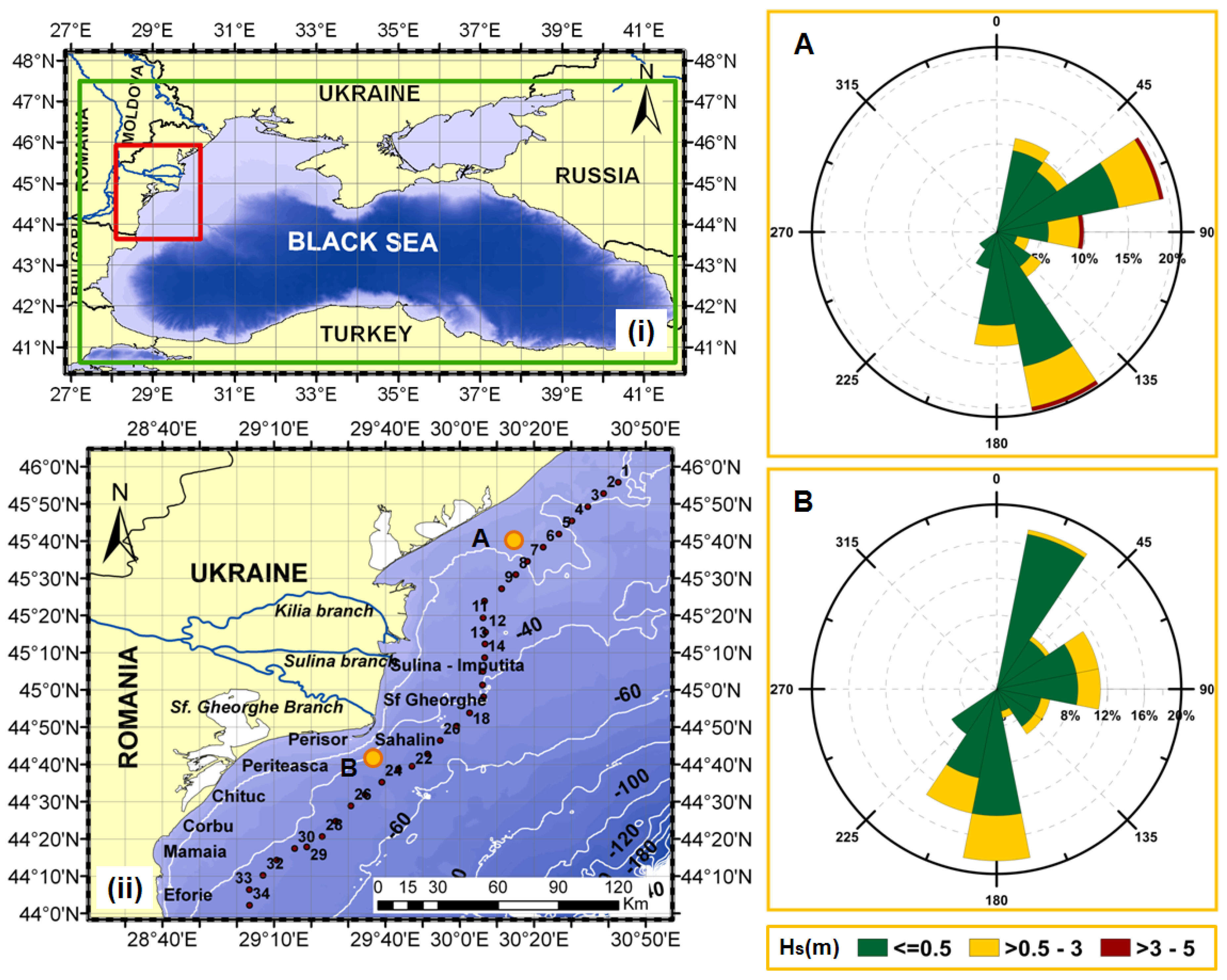
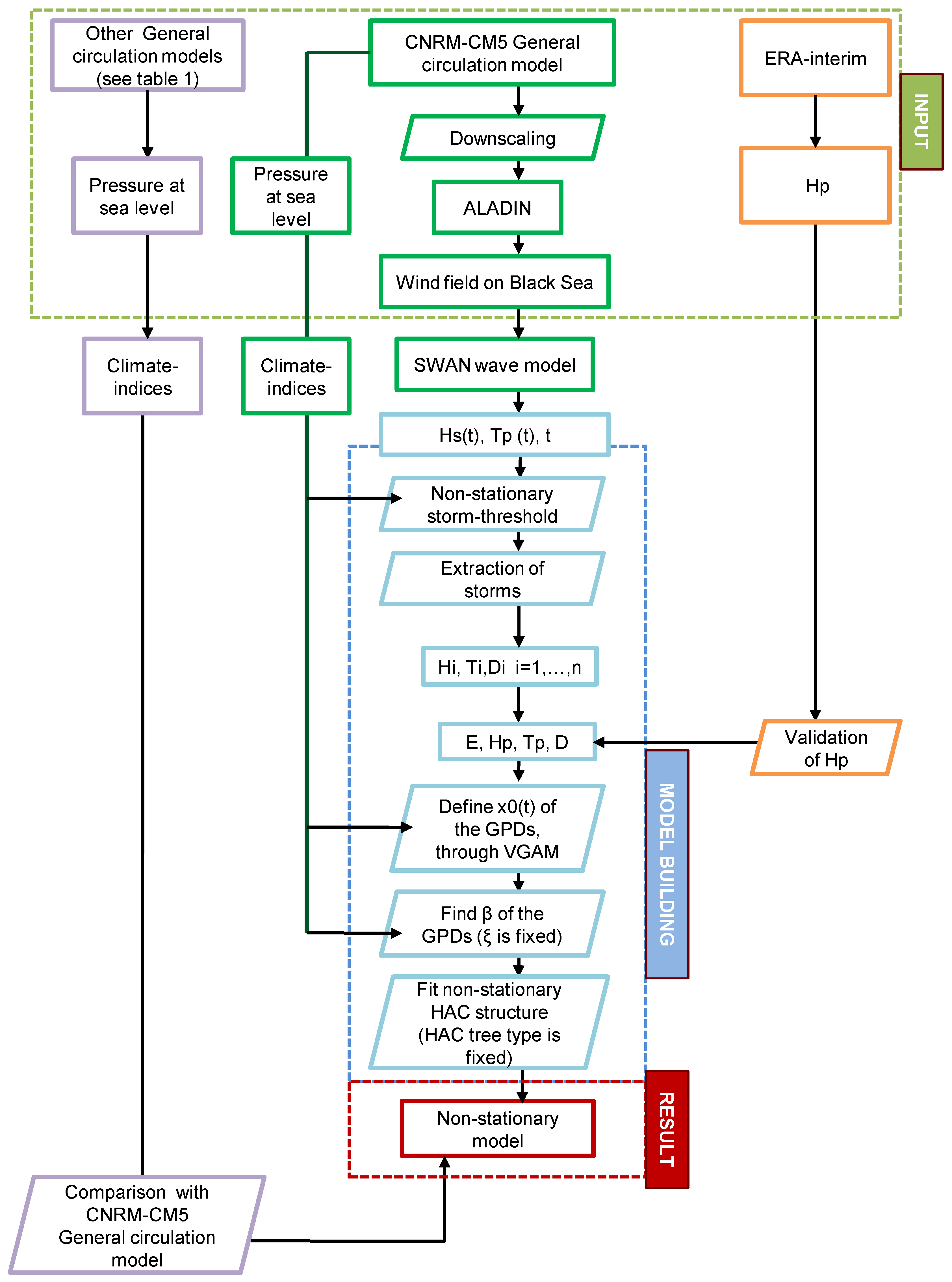
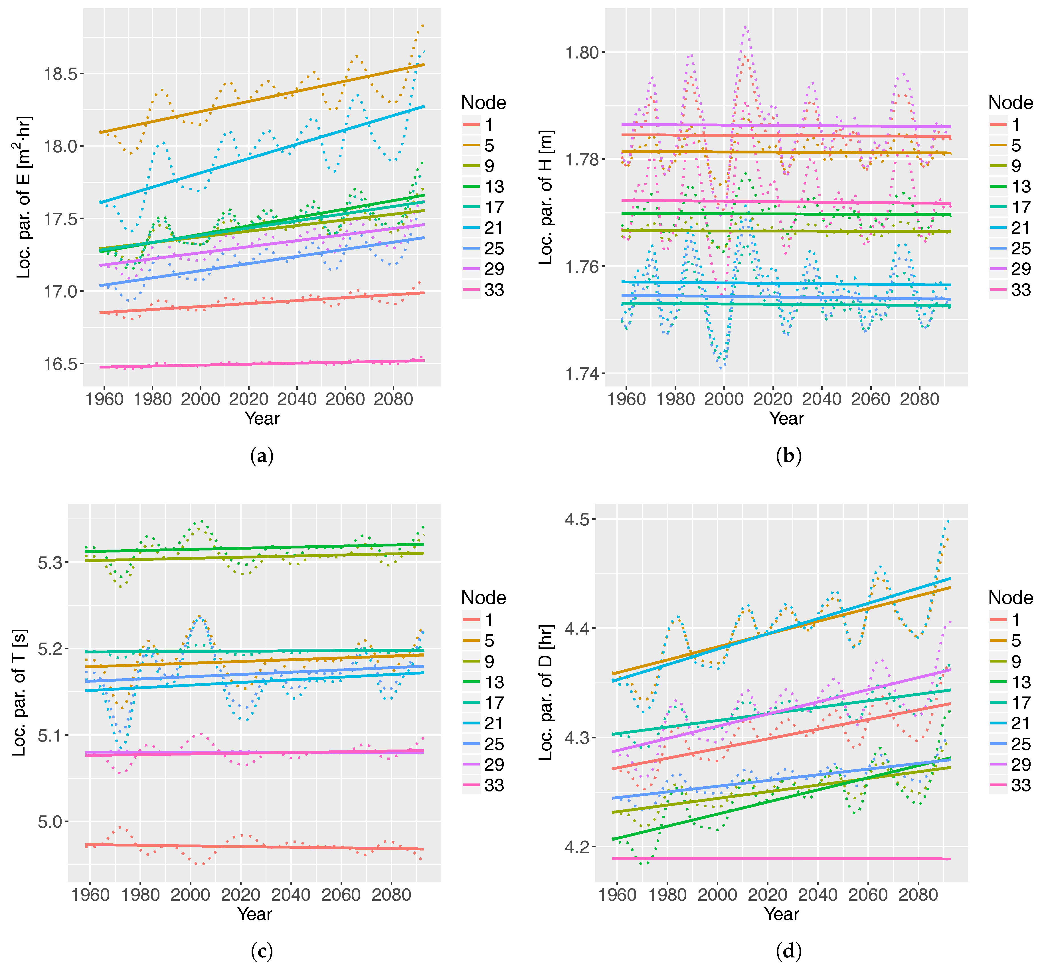
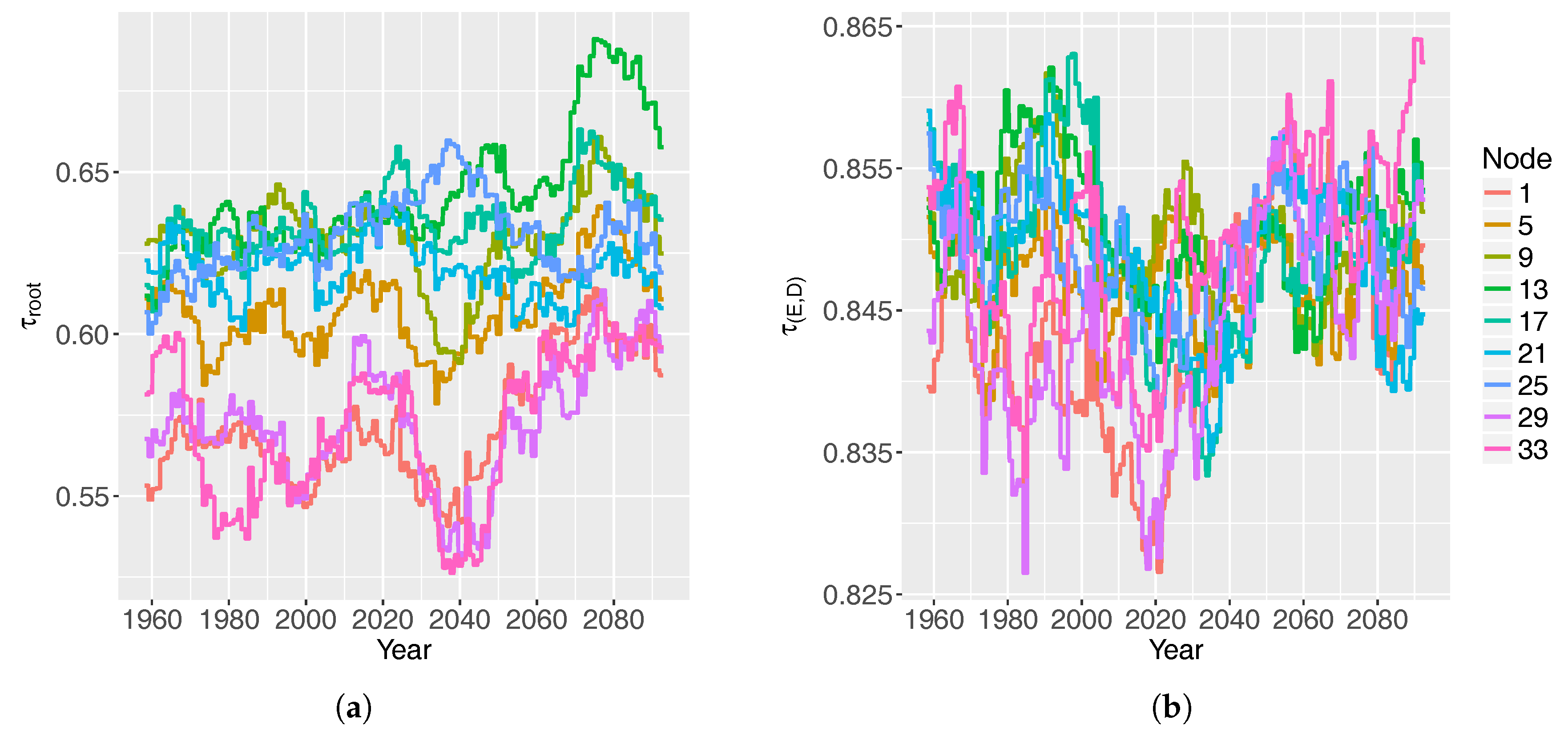
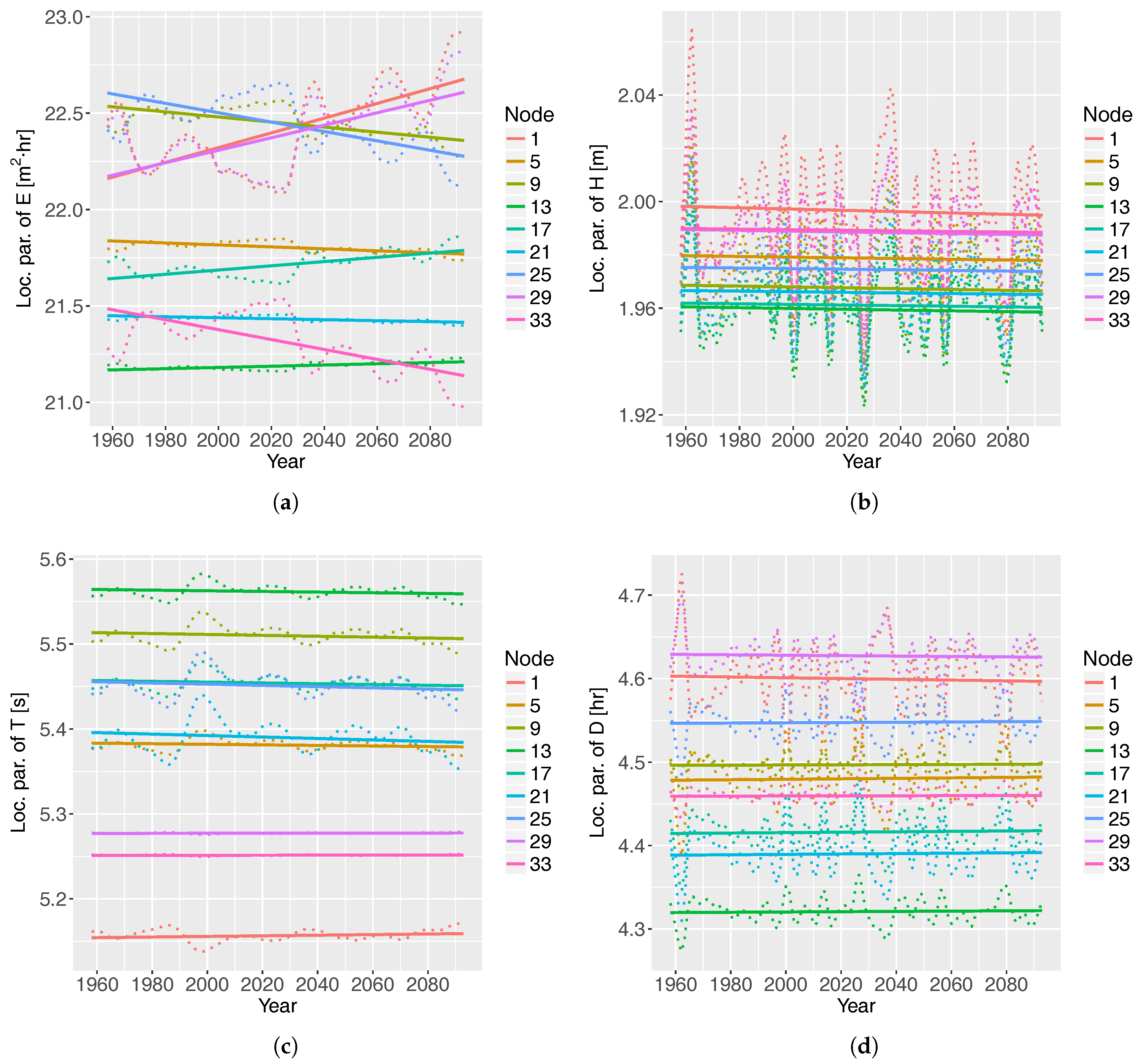
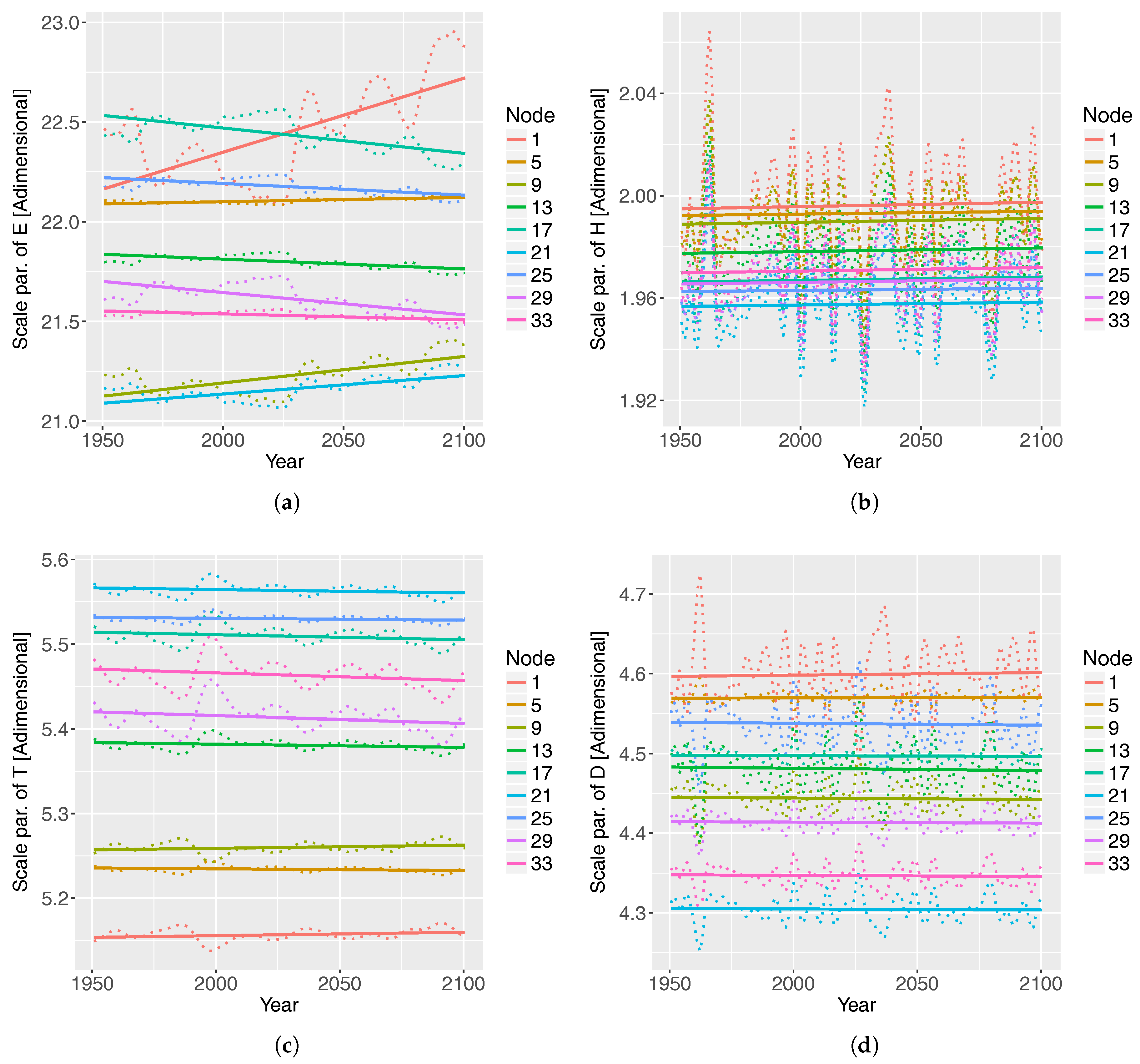
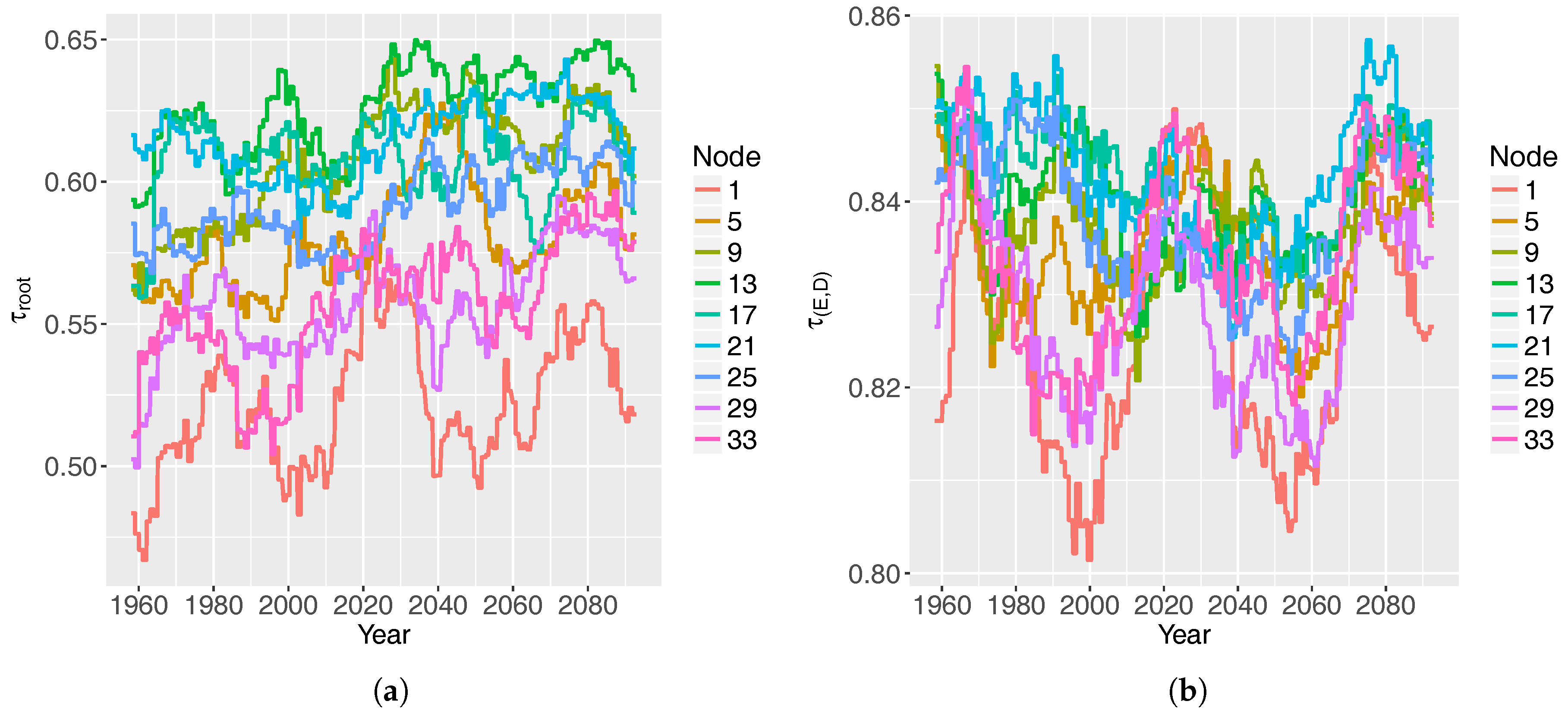
Table 1.
List of general circulation models (GCM) employed. The GCM CNRM-CM5 is used to build the non-stationary statistical model, whereas the other GCMs are compared to CNRM-CM5. CNRM-CM5 is shown in boldface to ease its search in the list.
Table 1.
List of general circulation models (GCM) employed. The GCM CNRM-CM5 is used to build the non-stationary statistical model, whereas the other GCMs are compared to CNRM-CM5. CNRM-CM5 is shown in boldface to ease its search in the list.
| GCM | Latitude | Longitude |
|---|---|---|
| Grid Size () | Grid Size () | |
| CMCC-CM | 0.7484 | 0.7500 |
| CMCC-CMS | 3.7111 | 3.7500 |
| CNRM-CM5 | 1.4008 | 1.4063 |
| FGOALS-G2 | 2.7906 | 2.8125 |
| GFDL-CM3 | 2.0000 | 2.5000 |
| GFDL-ESM2G | 2.0225 | 2.0000 |
| GFDL-ESM2M | 2.0225 | 2.5000 |
| HadGEM2-AO | 1.2500 | 1.8750 |
| HadGEM2-CC | 1.2500 | 1.8750 |
| HadGEM2-ES | 1.2500 | 1.8750 |
| INM-CM4 | 1.5000 | 2.0000 |
| IPSL-CM5A-LR | 1.8947 | 3.7500 |
| IPSL-CM5B-LR | 1.8947 | 3.7500 |
| IPSL-CM5A-MR | 1.2676 | 2.5000 |
| MIROC-ESM | 2.7906 | 2.8125 |
| MIROC-ESM-CHEM | 2.7906 | 2.8125 |
| MIROC5 | 1.4008 | 1.4063 |
| MPI-ESM-LR | 1.8653 | 1.8750 |
| MPI-ESM-MR | 1.8653 | 1.8750 |
Table 2.
Summary table of the Discussion section. and are the first and second time-derivatives, respectively.
Table 2.
Summary table of the Discussion section. and are the first and second time-derivatives, respectively.
| Variable or Test | Parameter | RCP4.5 | RCP8.5 |
|---|---|---|---|
| Main Covariate | |||
| Estimated storminess | 27–35 storms/year | 23–32 storms/year | |
| Storminess | None | None | |
| Wave-storm threshold | |||
| E | EA | None | |
| None | None | ||
| EA | SC | ||
| SC | NAO | ||
| EA | |||
| D | EA | None | |
| EA | |||
| – | – | ||
| – | – | ||
| HAC is non-stationary? | Yes | Yes | |
| Validated for 1979–2016? | Yes | Yes | |
© 2018 by the authors. Licensee MDPI, Basel, Switzerland. This article is an open access article distributed under the terms and conditions of the Creative Commons Attribution (CC BY) license (http://creativecommons.org/licenses/by/4.0/).
Share and Cite
MDPI and ACS Style
Lin-Ye, J.; García-León, M.; Gràcia, V.; Ortego, M.I.; Stanica, A.; Sánchez-Arcilla, A. Multivariate Hybrid Modelling of Future Wave-Storms at the Northwestern Black Sea. Water 2018, 10, 221. https://doi.org/10.3390/w10020221
AMA Style
Lin-Ye J, García-León M, Gràcia V, Ortego MI, Stanica A, Sánchez-Arcilla A. Multivariate Hybrid Modelling of Future Wave-Storms at the Northwestern Black Sea. Water. 2018; 10(2):221. https://doi.org/10.3390/w10020221
Chicago/Turabian StyleLin-Ye, Jue, Manuel García-León, Vicente Gràcia, M. Isabel Ortego, Adrian Stanica, and Agustín Sánchez-Arcilla. 2018. "Multivariate Hybrid Modelling of Future Wave-Storms at the Northwestern Black Sea" Water 10, no. 2: 221. https://doi.org/10.3390/w10020221
Note that from the first issue of 2016, this journal uses article numbers instead of page numbers. See further details here.