Hydrological Responses to Various Land Use, Soil and Weather Inputs in Northern Lake Erie Basin in Canada


 , ,
, ,
Abstract
:1. Introduction
2. Materials and Methods
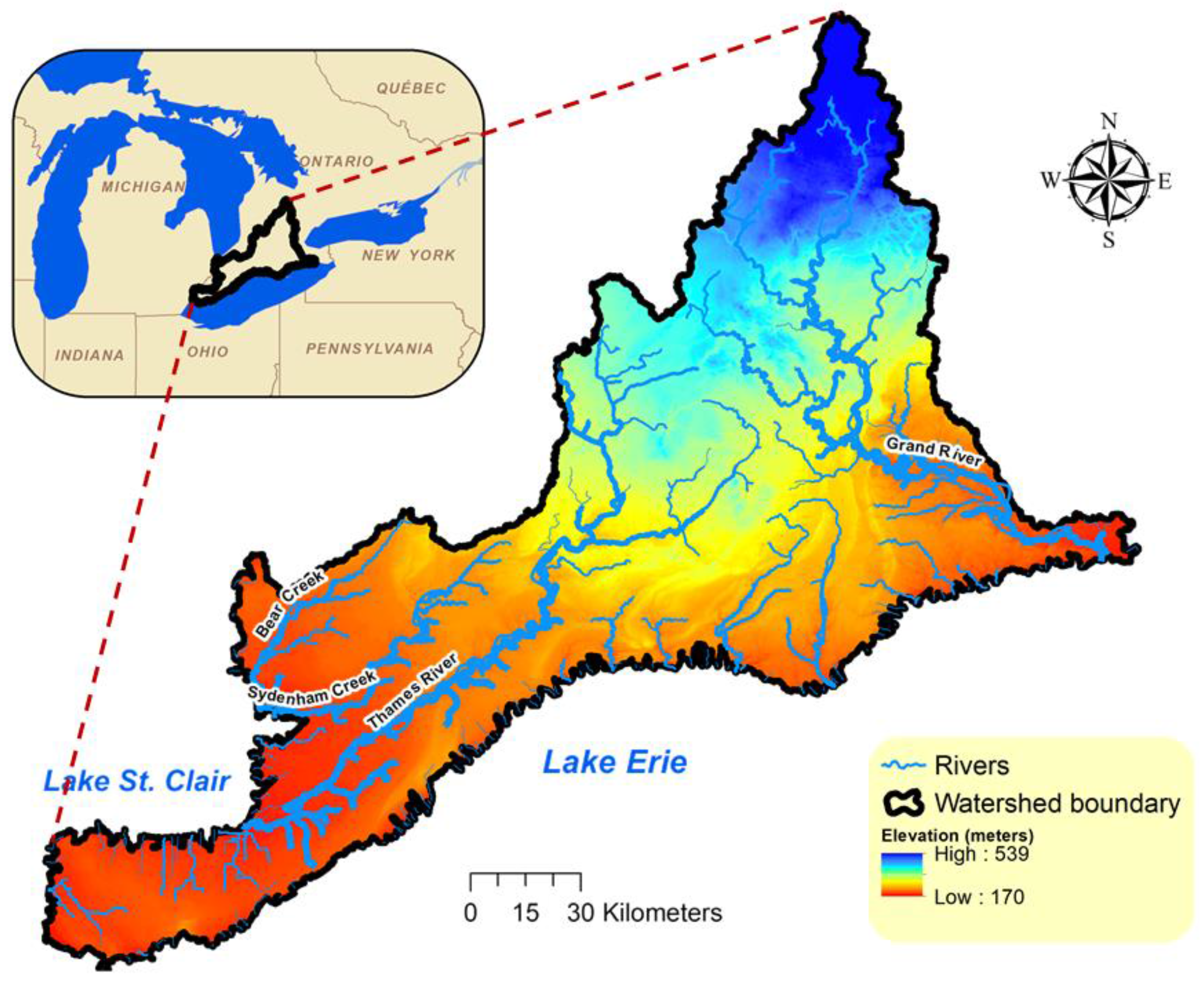
2.1. Study Area
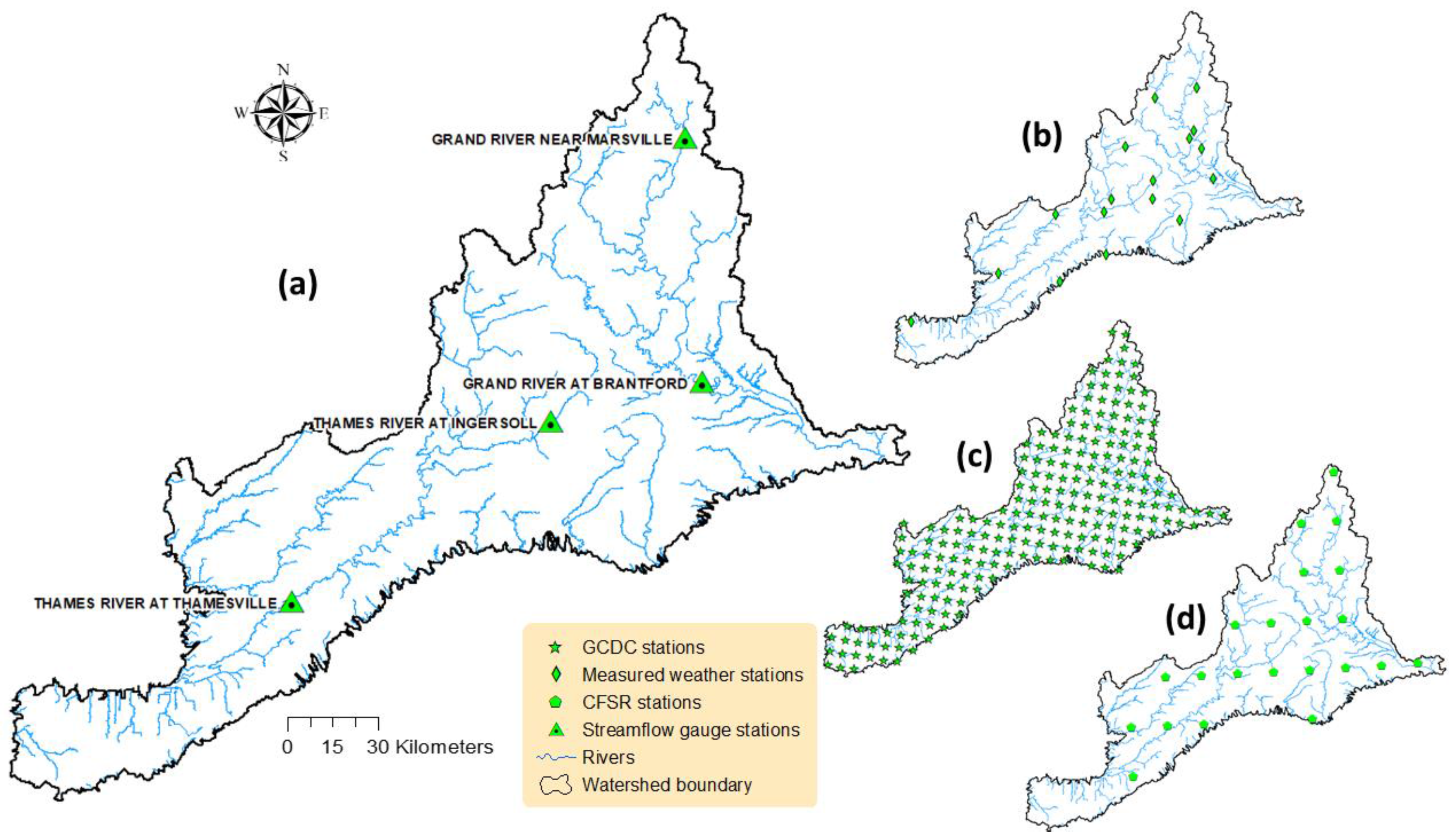
2.2. Input Data
2.2.1. DEM
2.2.2. Land Use and Land Cover
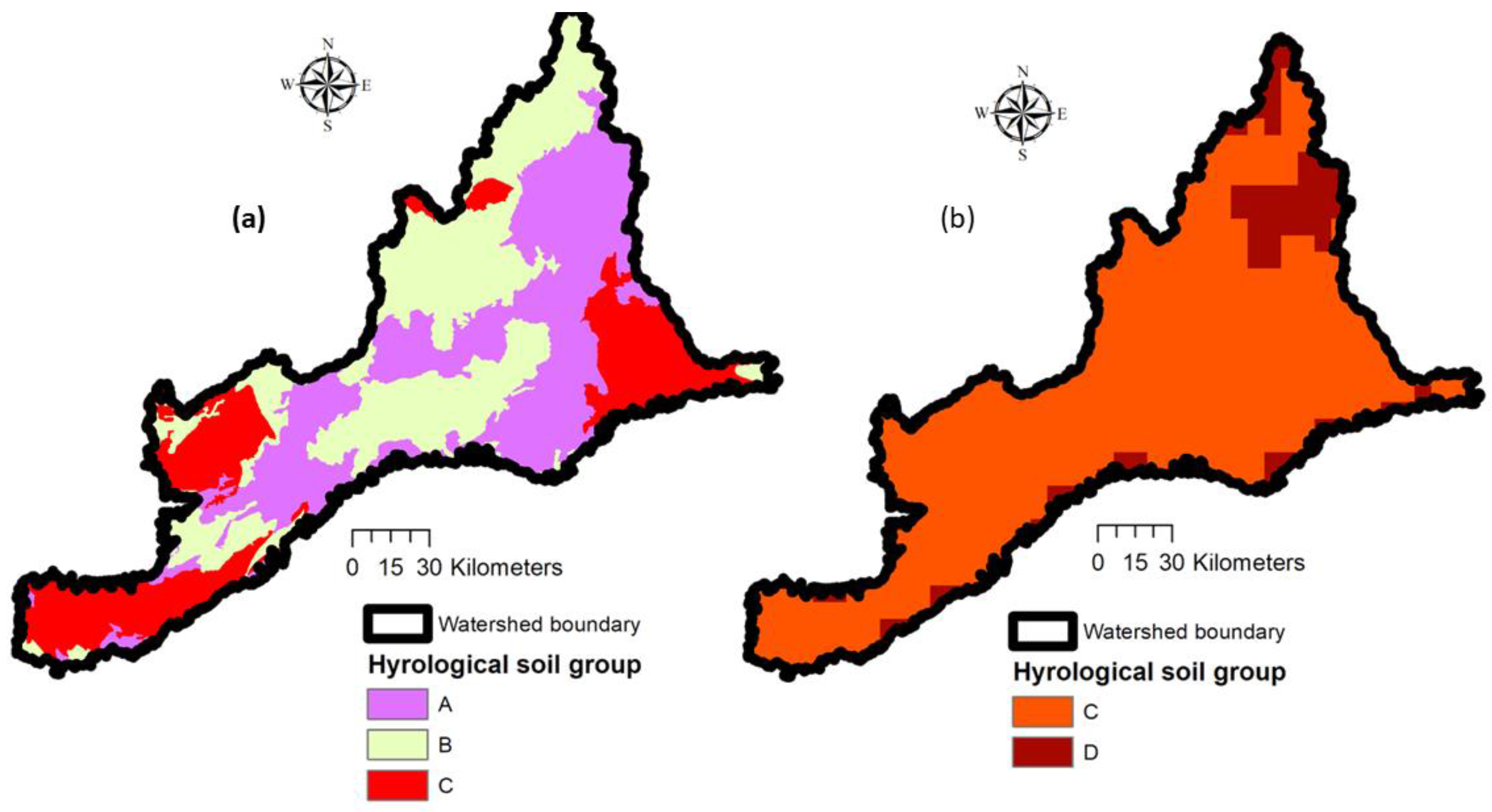
2.2.3. Soil
2.2.4. Weather
2.3. SWAT Model and Scenario Development
2.4. Input Data Assessment
3. Results and Discussion
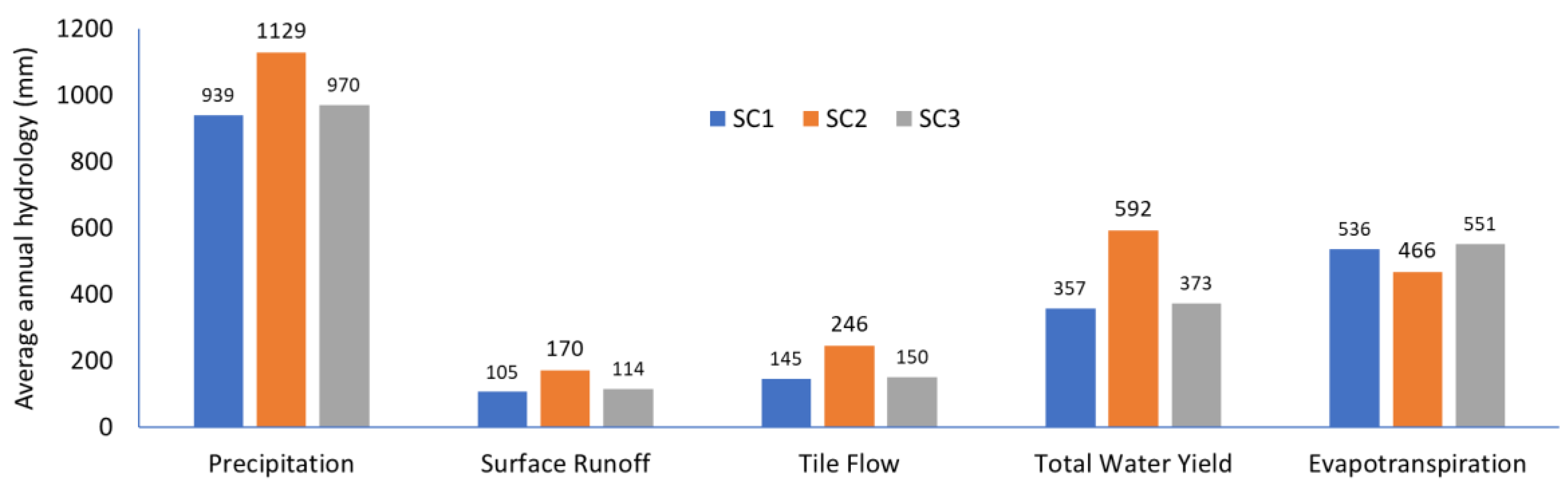
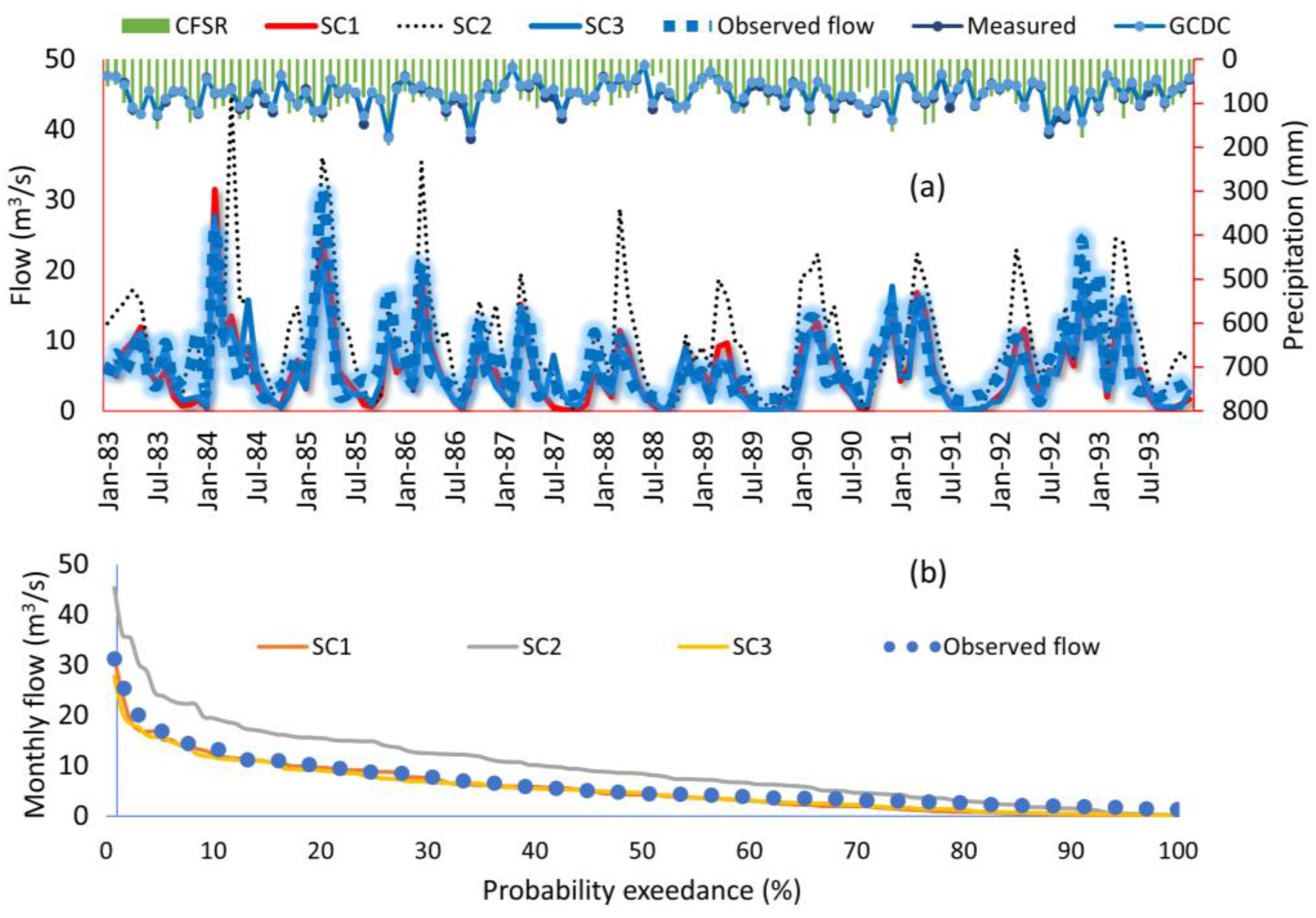
3.1. Compare Different Climate Datasets Using Hydrological Budgets and Measured Streamflow
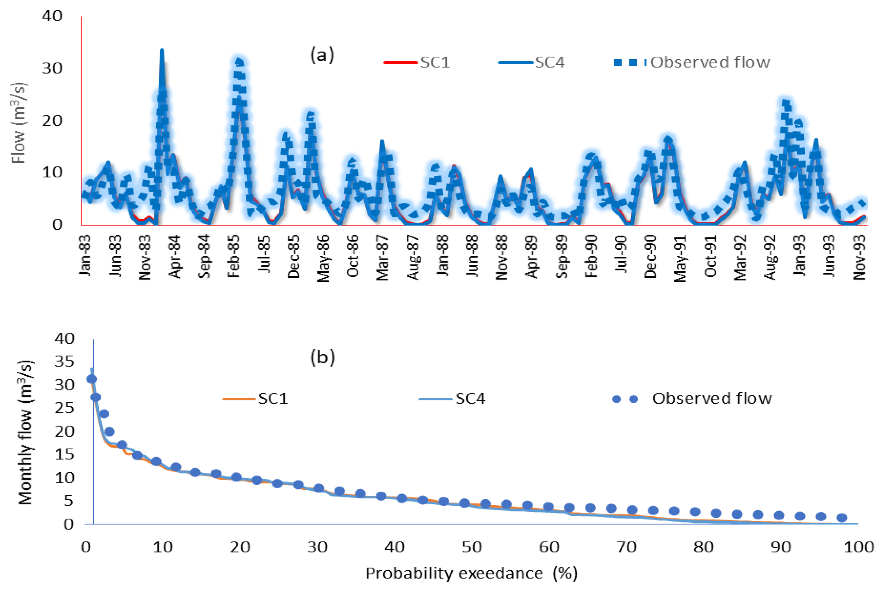
3.2. Comparison of Land Uses Using Hydrological Budgets and Measured Streamflow
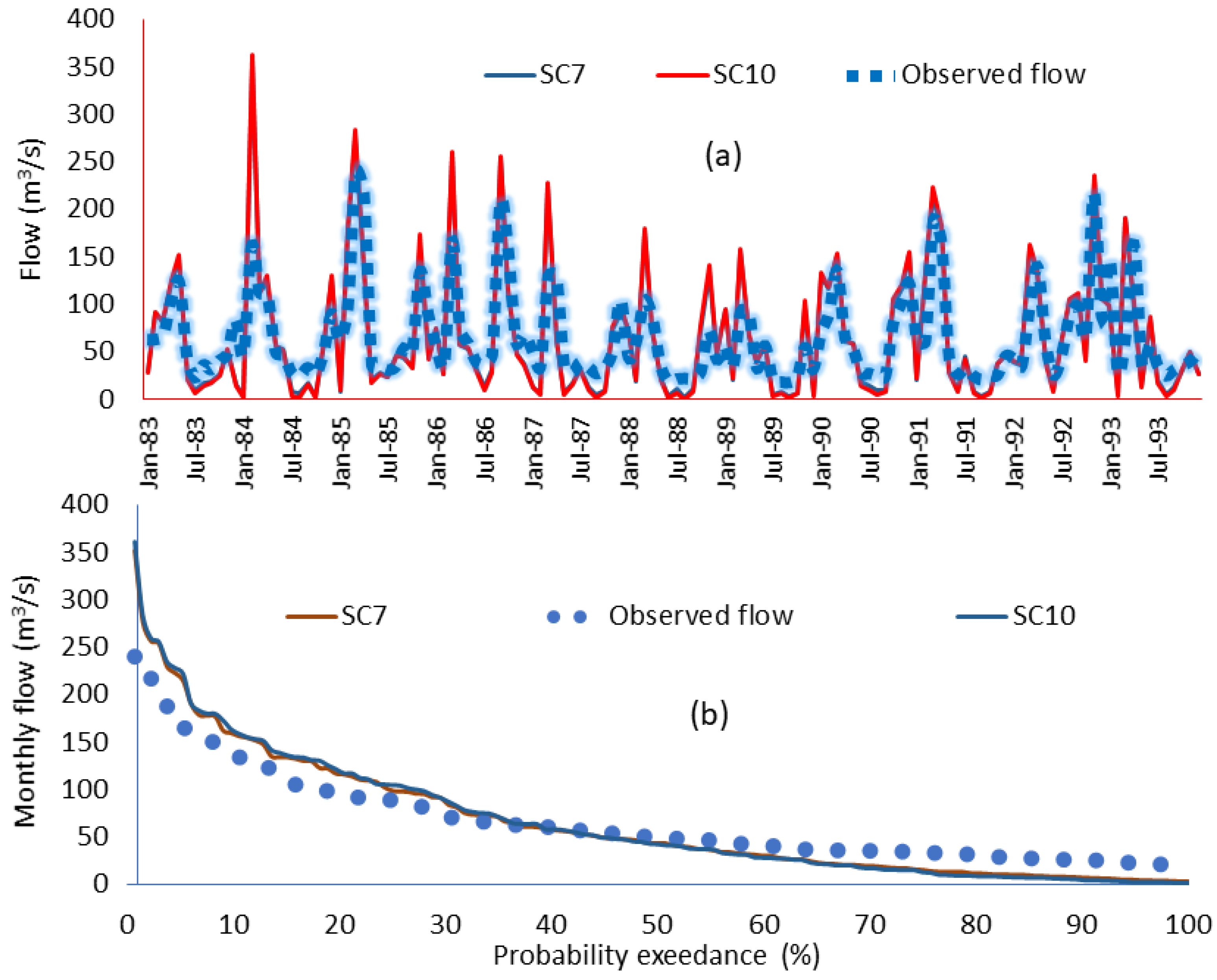
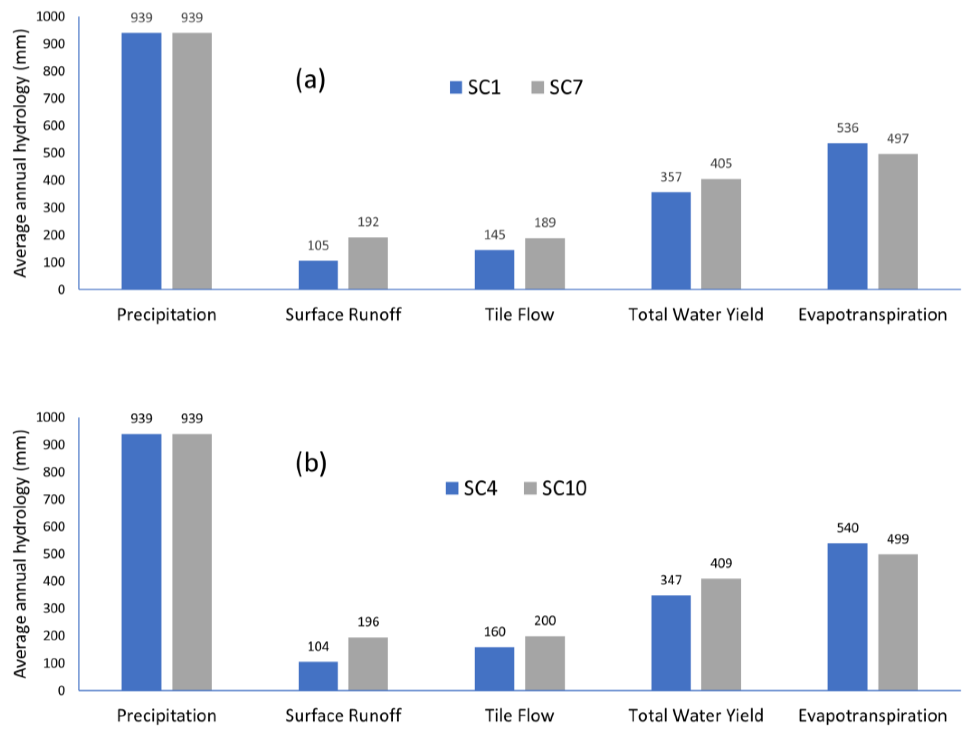
3.3. Impact of Soil on Hydrological Budgets and Streamflow
4. Conclusions
Acknowledgments
Author Contributions
Conflicts of Interest
References
- Cayton Andrew, R.L.; Sisson, R.; Zacher, C. The American Midwest: An Interpretive Encyclopedia; Indiana University Press: Bloomington, IN, USA, 2006; p. 161. ISBN 978-0-253-00349-2. [Google Scholar]
- Rucinski, D.K.; Beletsky, D.; DePinto, J.V.; Schwab, D.J.; Scavia, D. A simple 1-dimensional, climate based dissolved oxygen model for the central basin of Lake Erie. J. Gt. Lakes Res. 2010, 36, 465–476. [Google Scholar] [CrossRef]
- Dolan, D.M.; Chapra, S.C. Great Lakes total phosphorus revisited: 1. Loading analysis and update (1994–2008). J. Gt. Lakes Res. 2012, 38, 730–740. [Google Scholar] [CrossRef]
- Michalak, A.M.; Anderson, E.J.; Beletsky, D.; Boland, S.; Bosch, N.S.; Bridgeman, T.B.; Chaffin, J.D.; Cho, K.; Confesor, R.; Daloğlu, I.; et al. Record-setting algal bloom in Lake Erie caused by agricultural and meteorological trends consistent with expected future conditions. Proc. Natl. Acad. Sci. USA 2013, 110, 6448–6452. [Google Scholar] [CrossRef] [PubMed]
- Scavia, D.; Allan, J.D.; Arend, K.K.; Bartell, S.; Beletsky, D.; Bosch, N.S.; Brandt, S.B.; Briland, R.D.; Daloğlu, I.; DePinto, J.V.; et al. Assessing and addressing the re-eutrophication of Lake Erie: Central basin hypoxia. J. Gt. Lakes Res. 2014, 40, 226–246. [Google Scholar] [CrossRef]
- Watson, S.B.; Miller, C.; Arhonditsis, G.; Boyer, G.L.; Carmichael, W.; Charlton, M.N.; Confesor, R.; Depew, D.C.; Höök, T.O.; Ludsin, S.A.; et al. The re-eutrophication of Lake Erie: Harmful algal blooms and hypoxia. Harmful Algae 2016, 56, 44–66. [Google Scholar] [CrossRef] [PubMed]
- Arnold, J.G.; Srinivasan, R.; Muttiah, R.S.; Williams, J.R. Large-Area Hydrologic Modeling and Assessment: Part I. Model Development. J. Am. Water Resour. Assoc. 1998, 34, 73–89. [Google Scholar] [CrossRef]
- Gassman, P.W.; Reyes, M.R.; Green, C.H.; Arnold, J.G. The Soil and Water Assessment Tool: Historical Development, Applications, and Future Research Directions. Trans. ASABE 2007, 50, 1211–1250. [Google Scholar] [CrossRef]
- Bosch, N.S.; Allan, J.D.; Dolan, D.M.; Han, H.; Richards, R.P. Application of the Soil and Water Assessment Tool for six watersheds of Lake Erie: Model parameterization and calibration. J. Gt. Lakes Res. 2011, 37, 263–271. [Google Scholar] [CrossRef]
- Qi, C.; Grunwald, S. GIS-Based Hydrologic Modeling in the Sandusky Watershed Using SWAT. Trans. ASAE 2005, 48, 169–180. [Google Scholar] [CrossRef]
- Bosch, N.S.; Allan, J.D.; Selegean, J.P.; Scavia, D. Scenario-testing of agricultural best management practices in Lake Erie watersheds. J. Gt. Lakes Res. 2013, 39, 429–436. [Google Scholar] [CrossRef]
- Daggupati, P.; Yen, H.; White, M.J.; Srinivasan, R.; Arnold, J.G.; Keitzer, C.S.; Sowa, S.P. Impact of model development, calibration and validation decisions on hydrological simulations in West Lake Erie Basin. Hydrol. Process. 2015, 29, 5307–5320. [Google Scholar] [CrossRef]
- Yen, H.; Keitzer, S.C.; Daggupati, P.; Arnold, J.G.; Atwood, J.D.; Herbert, M.E.; Johnson, M.; Ludsin, S.A.; Srinivan, R.; Sowa, R.; Robertson, D.M. Soft-data-constrained, NHDPlus resolution watershed modeling and exploration of applicable conservation scenarios. Sci. Total Env. 2016, 569–570, 1265–1281. [Google Scholar] [CrossRef]
- Yen, H.; Daggupati, P.; White, M.J.; Srinivasan, R.; Arnold, J.G. Application of Large-Scale, Multi-resolution Watershed Modeling Framework Using the Hydrologic and Water Quality System (HAWQS). Water 2016, 8, 164. [Google Scholar] [CrossRef]
- Yang, W.; Liu, Y.; Ou, C.; Gabor, S. Examining water quality effects of riparian wetland loss and restoration scenarios in a southern Ontario watershed. J. Environ. Manag. 2016, 174, 26–34. [Google Scholar] [CrossRef] [PubMed]
- Golmohammadi, G.; Rudra, R.; Prasher, S.; Madani, A.; Mohammadi, K.; Goel, P.; Daggupati, P. Water Budget in a Tile Drained Watershed under Future Climate Change Using SWATDRAIN Model. Climate 2017, 5, 39. [Google Scholar] [CrossRef]
- Shao, H.; Yang, W.; Lindsay, J.; Liu, Y.; Yu, Z.; Oginskyy, A. An Open Source GIS-Based Decision Support System for Watershed Evaluation of Best Management Practices. J. Am. Water Resour. Assoc. 2017, 53, 521–531. [Google Scholar] [CrossRef]
- Liu, Y.B.; Yang, W.; Leon, L.; Wong, I.; McCrimmon, C.; Dove, A.; Fong, P. Hydrologic modeling and evaluation of Best Management Practice scenarios for the Grand River watershed in Southern Ontario. J. Gt. Lakes Res. 2016, 42, 1289–1301. [Google Scholar] [CrossRef]
- Olivera, F.; Valenzuela, M.; Srinivasan, R.; Choi, J.; Cho, H.; Koka, S.; Agrawal, A. ArcGIS-SWAT: A geodata model and GIS interface for SWAT. J. Am. Water Resour. Assoc. 2006, 42, 295–309. [Google Scholar] [CrossRef]
- Romanowicz, A.A.; Vanclooster, M.; Rounsevell, M.; La Jeunesse, I. Sensitivity of the SWAT model to the soil and land use data parameterisation: A case study in the Thyle catchment, Belgium. Ecol. Model. 2005, 187, 27–39. [Google Scholar] [CrossRef]
- Daggupati, P.; Douglas-Mankin, K.R.; Sheshukov, A.Y.; Barnes, P.L.; Devlin, D.L. Field-Level Targeting Using SWAT: Mapping Output from HRUs to Fields and Assessing Limitations of GIS Input Data. Trans. ASABE 2011, 54, 501–514. [Google Scholar] [CrossRef]
- Wang, X.; Melesse, A.M. Effects of STATSGO and SSURGO as inputs on SWAT model's snowmelt simulation. J. Am. Water Resour. Assoc. 2006, 42, 1217–1236. [Google Scholar] [CrossRef]
- Peschel, J.M.; Haan, P.K.; Lacey, R. EInfluences of soil dataset resolution on hydrologic modeling. J. Am. Water Resour. Assoc. 2006, 42, 1371–1389. [Google Scholar] [CrossRef]
- USDA-NRCS. Soil Survey Geographic (SSURGO) Database; USDA Natural Resources Conservation Service: Washington, DC, USA, 2005.
- USDA-NRCS. State Soil Geographic (STATSGO) Database; USDA Natural Resources Conservation 514 Transactions of the ASABE Service: Washington, DC, USA, 1994.
- Heathman, G.C.; Larose, M.; Ascough, J.C. SWAT evaluation of soil and land use GIS data sets on simulated streamflow. J. Soil Water Conserv. 2009, 64, 17–32. [Google Scholar] [CrossRef]
- Radcliffe, D.E.; Mukundan, R. PRISM vs. CFSR precipitation data effects on calibration and validation of SWAT models. J. Am. Water Resour. Assoc. 2017, 53, 89–100. [Google Scholar] [CrossRef]
- Gao, J.; Sheshukov, A.Y.; Yen, H.; White, M.J. Impacts of alternative climate information on hydrologic processes with SWAT: A comparison of NCDC, PRISM and NEXRAD datasets. Catena 2017, 156, 353–364. [Google Scholar] [CrossRef]
- Hansen, M.C.; Defries, R.S.; Townshend, J.R.G.; Sohlberg, R. Global land cover classification at 1 km spatial resolution using a classification tree approach. Int. J. Remote Sens. 2000, 21, 1331–1364. [Google Scholar] [CrossRef]
- The Ontario Ministry of Natural Resources. Southern Ontario Land Resource Information System (SOLRIS) Land Classification Data; Version 1.2; The Ontario Ministry of Natural Resources: Peterborough, ON, Canada, 2008.
- Loveland, T.R.; Reed, B.C.; Brown, J.F.; Ohlen, D.O.; Zhu, Z.; Yang, L.W.M.J.; Merchant, J.W. Development of a global land cover characteristics database and IGBP DISCover from 1 km AVHRR data. Int. J. Remote Sens. 2000, 21, 1303–1330. [Google Scholar] [CrossRef]
- Lee, H.T.; Bakowsky, W.; Riley, J.; Bowles, J.; Puddister, M.; Uhlig, P. Ecological Land Classification for Southern Ontario: First Approximation and Its Application; Ontario Ministry of Natural Resources; Southcentral Science Section: North Bay, ON, Canada, 1998.
- Soil Landscapes of Canada Working Group. Soil Landscapes of Canada v3. 1.1 Agriculture and Agri-Food Canada. Digital Map and Database at 1:1 Million Scale. Available online: http://sis.agr.gc.ca/cansis/nsdb/slc/v3.1.1/intro.html (accessed on 1 June 2017).
- Hutchinson, M.F.; McKenney, D.W.; Lawrence, K.; Pedlar, J.H.; Hopkinson, R.F.; Milewska, E.; Papadopol, P. Development and testing of Canada-wide interpolated spatial models of daily minimum–maximum temperature and precipitation for 1961–2003. J. Appl. Meteorol. Climatol. 2009, 48, 725–741. [Google Scholar] [CrossRef]
- Saha, S.; Moorthi, S.; Pan, H.L.; Wu, X.; Wang, J.; Nadiga, S.; Liu, H. The NCEP climate forecast system reanalysis. Bull. Am. Meteorol. Soc. 2010, 91, 1015–1057. [Google Scholar] [CrossRef]
- Dile, Y.T.; Srinivasan, R. Evaluation of CFSR climate data for hydrologic prediction in data-scarce watersheds: An application in the Blue Nile River Basin. J. Am. Water Resour. Assoc. 2014, 50, 1226–1241. [Google Scholar] [CrossRef]
- Bressiani, D.D.A.; Gassman, P.W.; Fernandes, J.G.; Garbossa, L.H.P.; Srinivasan, R.; Bonumá, N.B.; Mendiondo, E.M. A review of SWAT (Soil and Water Application Tool) applications in Brazil: Challenges and prospects. Int. J. Agric. Biol. Eng. 2015, 8, 9–35. [Google Scholar] [CrossRef]
- Fuka, D.R.; Walter, M.T.; MacAlister, C.; Degaetano, A.T.; Steenhuis, T.S.; Easton, Z.M. Using the climate forecast system reanalysis as weather input data for watershed models. Hydrol. Process. 2016, 28, 5613–5623. [Google Scholar] [CrossRef]
- Daggupati, P.; Srinivasan, R.; Dile, Y.; Verma, D. Reconstructing the historical water regime of the contributing basins to the Hawizeh marsh: Implications of water control structures. Sci. Total. Environ. 2017, 580, 832–845. [Google Scholar] [CrossRef] [PubMed]
- Daggupati, P.; Pai, N.; Ale, S.; Douglas-mankin, K.R.; Zeckoski, R.W.; Jeong, J.; Parajuli, P.B.; Saraswat, D.; Youssef, M. Recommended calibration and validation strategy for hydrologic and water quality models. Trans. ASABE. 2015, 58, 1705–1719. [Google Scholar] [CrossRef]
- Moriasi, D.N.; Zeckoski, R.W.; Arnold, J.G.; Baffaut, C.; Malone, R.W.; Daggupati, P.; Shirmohammadi, A. Hydrologic and water quality models: Key calibration and validation topics. Trans. ASABE 2015, 58, 1609–1618. [Google Scholar] [CrossRef]
- Arnold, J.; Moriasi, D.; Gassman, P.; Abbaspour, K.; White, M.; Srinivasan, R.; Santhi, C.; Harmel, R.D.; van Griensven, A.; Van Liew, M.W.; et al. SWAT: Model use, calibration, and validation. Trans. ASABE. 2012, 55, 1491–1508. [Google Scholar] [CrossRef]
- Moriasi, D.N.; Gitau, M.W.; Pai, N.; Daggupati, P. Hydrologic and water quality models: Performance measures and evaluation criteria. Trans. ASABE 2015, 58, 1763–1785. [Google Scholar] [CrossRef]
- Gupta, H.V.; Sorooshian, S.; Yapo, P.O. Status of automatic calibration for hydrologic models: Comparison with multilevel expert calibration. J. Hydrol. Eng. 1999, 4, 135–143. [Google Scholar] [CrossRef]
- Khare, D.; Singh, R.; Shukla, R. Hydrological Modeling of Barinallah Watershed Using Arc SWAT model. Int. J. Geol. Earth Environ. Sci. 2014, 4, 224–235. [Google Scholar]
- Ayele, G.T.; Teshale, E.Z.; Yu, B.; Rutherfurd, I.D.; Jeong, J. Streamflow and sediment yield prediction for watershed prioritization in the Upper Blue Nile River Basin, Ethiopia. Water 2017, 9, 782. [Google Scholar] [CrossRef]


| Inputs | Resolution | Data Availability | Website |
|---|---|---|---|
| DEM | 30 m | Provincial | https://www.ontario.ca/data/provincial-digital-elevation-model-version-30 |
| Land use | |||
| GLCC | 1 km | Global | https://lta.cr.usgs.gov/GLCC |
| SOLRIS | 30 m | Provincial | https://www.ontario.ca/data/southern-ontario-land-resource-information-system-solris-20 |
| Soil | |||
| FAO | 5 km | Global | http://www.fao.org/soils-portal/soil-survey/soil-maps-and-databases/en/ |
| SLC | 1 km | National | http://sis.agr.gc.ca/cansis/nsdb/slc/v3.2/index.html |
| Weather | |||
| CFSR | 250 km | Global | https://globalweather.tamu.edu/ |
| GCDC | 10 km | National | http://www.agr.gc.ca/nlwis |
| Measured | -- | National | http://climate.weather.gc.ca/ |
| Scenario | Soil Data | Landuse Data | Climate Data |
|---|---|---|---|
| SC1 | SLC soil | SOLRIS landuse | GCDC |
| SC2 | SLC soil | SOLRIS landuse | CFSR |
| SC3 | SLC soil | SOLRIS landuse | Measured |
| SC4 | SLC soil | GLCC landuse | GCDC |
| SC5 | SLC soil | GLCC landuse | CFSR |
| SC6 | SLC soil | GLCC landuse | Measured |
| SC7 | FAO soil | SOLRIS landuse | GCDC |
| SC8 | FAO soil | SOLRIS landuse | CFSR |
| SC9 | FAO soil | SOLRIS landuse | Measured |
| SC10 | FAO soil | GLCC landuse | GCDC |
| SC11 | FAO soil | GLCC landuse | CFSR |
| SC12 | FAO soil | GLCC landuse | Measured |
| Gauge Stations | Grand at Brandford (G1) | Grand at Marsville (G2) | Thames at Ingresol (T1) | Thames at Thameville (T2) | ||||
|---|---|---|---|---|---|---|---|---|
| Scenarios | PBIAS (%) | NSE | PBIAS (%) | NSE | PBIAS (%) | NSE | PBIAS (%) | NSE |
| SC1 | 1.09 (VG) | 0.71 (G) | −5.94 (G) | 0.80 (G) | 13.56 (S) | 0.73 (G) | 6.05 (G) | 0.84 (VG) |
| SC2 | −65.19 (NS) | −1.42 (NS) | −70.70 (NS) | −0.09 (NS) | −50.72 (NS) | −0.69 (NS) | −52.76 (NS) | −0.27 (NS) |
| SC3 | −4.47 (VG) | 0.75 (G) | −2.86 (VG) | 0.70 (G) | 14.65 (S) | 0.70 (G) | 1.14 (VG) | 0.84 (VG) |
| SC4 | 3.59 (VG) | 0.68 (G) | −6.34 (G) | 0.81 (VG) | 15.43 (NS) | 0.70 (G) | 8.63 (G) | 0.82 (VG) |
| SC5 | −62.11 (NS) | −1.47 (NS) | −71.69 (NS) | −0.18 (NS) | −48.23 (NS) | −0.76 (NS) | −48.95 (NS) | −0.25 (NS) |
| SC6 | −1.77 (VG) | 0.74 (G) | −3.45 (VG) | 0.70 (G) | 16.71 (NS) | 0.68 (S) | 3.95 (VG) | 0.83 (VG) |
| SC7 | −0.47 (VG) | 0.36 (NS) | −12.51 (S) | 0.75 (G) | 5.87 (G) | 0.48 (NS) | −4.49 (VG) | 0.71 (G) |
| SC8 | −66.92 (NS) | −2.31 (NS) | −77.70 (NS) | −0.48 (NS) | −67.49 (NS) | −1.85 (NS) | −68.87 (NS) | −1.01 (NS) |
| SC9 | −5.50 (G) | 0.37 (NS) | −9.26 (G) | 0.53 (S) | 7.27 (G) | 0.44 (NS) | −10.19 (S) | 0.69 (S) |
| SC10 | −1.40 (VG) | 0.30 (NS) | −16.15 (NS) | 0.73 (G) | 4.15 (VG) | 0.50 (NS) | −5.77 (G) | 0.69 (S) |
| SC11 | −68.47 (NS) | −2.52 (NS) | −80.77 (NS) | −0.53 (S) | −69.45 (NS) | −2.01 (NS) | −70.43 (NS) | −1.13 (NS) |
| SC12 | −6.32 (G) | 0.32 (NS) | −13.29 (S) | 0.50 (NS) | 5.52 (G) | 0.40 (NS) | −11.46 (S) | 0.67 (S) |
© 2018 by the authors. Licensee MDPI, Basel, Switzerland. This article is an open access article distributed under the terms and conditions of the Creative Commons Attribution (CC BY) license (http://creativecommons.org/licenses/by/4.0/).
Share and Cite
Daggupati, P.; Shukla, R.; Mekonnen, B.; Rudra, R.; Biswas, A.; Goel, P.K.; Prasher, S.; Yang, W. Hydrological Responses to Various Land Use, Soil and Weather Inputs in Northern Lake Erie Basin in Canada. Water 2018, 10, 222. https://doi.org/10.3390/w10020222
Daggupati P, Shukla R, Mekonnen B, Rudra R, Biswas A, Goel PK, Prasher S, Yang W. Hydrological Responses to Various Land Use, Soil and Weather Inputs in Northern Lake Erie Basin in Canada. Water. 2018; 10(2):222. https://doi.org/10.3390/w10020222
Chicago/Turabian StyleDaggupati, Prasad, Rituraj Shukla, Balew Mekonnen, Ramesh Rudra, Asim Biswas, Pradeep K. Goel, Shiv Prasher, and Wanhong Yang. 2018. "Hydrological Responses to Various Land Use, Soil and Weather Inputs in Northern Lake Erie Basin in Canada" Water 10, no. 2: 222. https://doi.org/10.3390/w10020222