Responses of Bed Morphology to Vegetation Growth and Flood Discharge at a Sharp River Bend


Hydraulic Research Laboratory, Hokkaido University, Hokkaido 060-8628, Japan
*
Author to whom correspondence should be addressed.
Water 2018, 10(2), 223; https://doi.org/10.3390/w10020223
Submission received: 14 November 2017
/
Revised: 12 February 2018
/
Accepted: 16 February 2018
/
Published: 22 February 2018
(This article belongs to the Special Issue Water Resources and Environmental Fluid Mechanics: From the Glacier to the Lake/Ocean)
Abstract
:In this study, we conducted simulations using a two-dimensional, depth-averaged river flow and river morphology model to investigate the effect of vegetation growth and degree of flow discharge on a shallow meandering channel. To consider the effects of these factors, it was assumed that vegetation growth stage is changed by water flow and bed erosion. The non-uniformity of the vegetation growth was induced by the non-uniform and unsteady profile of the water depth due to the irregular shape of the bed elevation and the unsteady flow model reliant on hydrographs to evaluate three types of peak discharges: moderate flow, annual average maximum flow, and extreme flow. To compare the effects of non-uniform growing vegetation, the change in channel patterns was quantified using the Active Braiding Index (ABI), which indicates the average number of channels with flowing water at a cross section and the Bed Relief Index (BRI), which quantifies the degree of irregularity of the cross-sectional shape. Two types of erosion were identified: local erosion (due to increased flow velocity near a vegetation area) and global erosion (due to the discharge approaching peak and the large depth of the channel). This paper demonstrated that the growth of vegetation increases both the ABI and BRI when the peak discharge is lower than the annual average discharge, whereas the growth of vegetation reduces the BRI when the peak discharge is extreme. However, under extreme discharge, the ABI decreases because global erosion is dominant. The conclusions from this study help to deepen the understanding of the interactions between curved river channels and vegetation.
1. Introduction
Channel meander and vegetation growth are important factors influencing river morphology. Vegetation, in particular, is one of the main friction factors in shallow water flow. An area of vegetation alters river flow profiles by contributing to the increase in the water depth, decrease in the flow velocity, and increase in the shear stress near the vegetation, among other effects.
The growth of vegetation plays many diverse roles in river environments beyond simply disturbing the flood flow path. In particular, it influences sediment transport patterns. Several researchers have described the effects of vegetation on sediment transport, which contributes to the deformation of a riverbed [1,2,3]. Several experiments [4,5,6,7,8], numerical simulations [9,10,11], and field studies [12,13,14,15] have shown that vegetation influences changes in channel flow and sediment transport.
Vegetation frequently affects the meandering of channels because vegetation reinforces the channel bank and reduces the number of active channels by inducing changes in sediment transport [4,5,7,9,16]. The relationship between vegetation and channel meander is therefore one of the most important factors in understanding the morphology of rivers [6,17,18,19,20,21,22,23].
Until now, many field studies related to the interaction between vegetation effect and bed morphology have been actively carried out and these have provided useful data for a developing model of the vegetation effect in river alteration [12,13,14,15]. By employing such field survey data, conceptual models and statistical models that can consider diverse parameters such as flow discharge, sediment, and channel form have been proposed and the relationship among vegetation, water flow, and bed morphology have been presented for river bed change by riparian vegetation [12,13]. Gurnell and Grabowski [14] investigated the importance of potential vegetation effect under the dynamics of bed morphology for river management and restoration. Abernethy et al. [15] studied the relation between the root characteristics and bank stabilization, and their results specifically show how the stability of the bank is affected by root profile.
In the past several years, numerical simulations and experiments have been conducted to investigate the effects of vegetation on open channel flows [24,25,26]. In particular, two-dimensional computations have been mainly used for such studies, because it is obvious that two-dimensional computations are more efficient than three-dimensional types if the grid spatial resolution in the horizontal plane are the same. For example, Tsujimoto [27] surveyed river-bed deformation by means of a depth-averaged two-dimensional numerical model with added vegetation terms in the momentum and turbulent flow equations. The results demonstrate that the length of a vegetated free bar increases with exposure to an increased frequency of flood events. Crosato and Saleh [28] simulated the long-term deformation of a river bed for varying degrees of vegetation density in the flood plain using a two-dimensional numerical model. It was found that a braided channel develops more readily when there is no vegetation; with sufficient density, vegetation contributes to the formation of a single thread channel.
Many researchers have conducted experiments to study the effects of vegetation on river channels through uniformly distributed seeding and growing [4,5,6,7,29]. These studies demonstrate that a river bank with settled vegetation is sufficiently protected from erosion. Moreover, the number of thread channels decreases and the ratio of channel width to water depth decreases due to the effects of the vegetation, which contributes to the maintenance of the meandering channel. However, these previous studies considered only conditions of steady flow, which exclude, by definition, flood plain inundations, and only local erosion in the low channel is dominant. In Korea, vegetation growth is generally highly active during flood season (spring to summer), indicating that the effects of vegetation on the behavior of a river subject to flood conditions are critical considerations in understanding river morphology. Considering this research background, we investigated the effects of vegetation on river morphology using numerical methods. In most of the existing numerical investigations in the literature, the non-uniform growth of vegetation in response to unsteady flow was not investigated as most studies assumed static vegetation. Consequently, most published research insufficiently explained changes to river bed morphology in response to the changes in vegetation growth that accompany flood events. Van Dijk et al. [8] also pointed out that it is important to consider the distribution of vegetation because most experimental studies investigate small-scale bed morphology using uniform seed deposition; however, vegetation distribution is likely disrupted by flood events in the river channel.
Therefore, it is necessary to consider the process of non-uniform vegetation growth under conditions of unsteady flow, including growth, colonization, and decay states subject to flood events. Perucca et al. [10] and Ye et al. [30] suggested that the two main factors that influence the morphology of a meandering river with riparian vegetation are the degree of vegetation colonization and the alteration of flow discharge resulting from events such as floods, and droughts [31,32,33,34,35]. However, the mechanism of bed morphology changes in response to the growth of vegetation remains unclear.
Indeed, the effect of vegetation in a meandering channel indicates a different behavioral phase than what is present in a straight channel. Garcia et al. [36] emphasized that meandering channels have highly complex morphodynamical elements that control the ecosystems in the river basin. Therefore, it is important to include the presence of both vegetation and curved channel, because the vegetation and the meandering channel interact to maintain dynamic equilibrium.
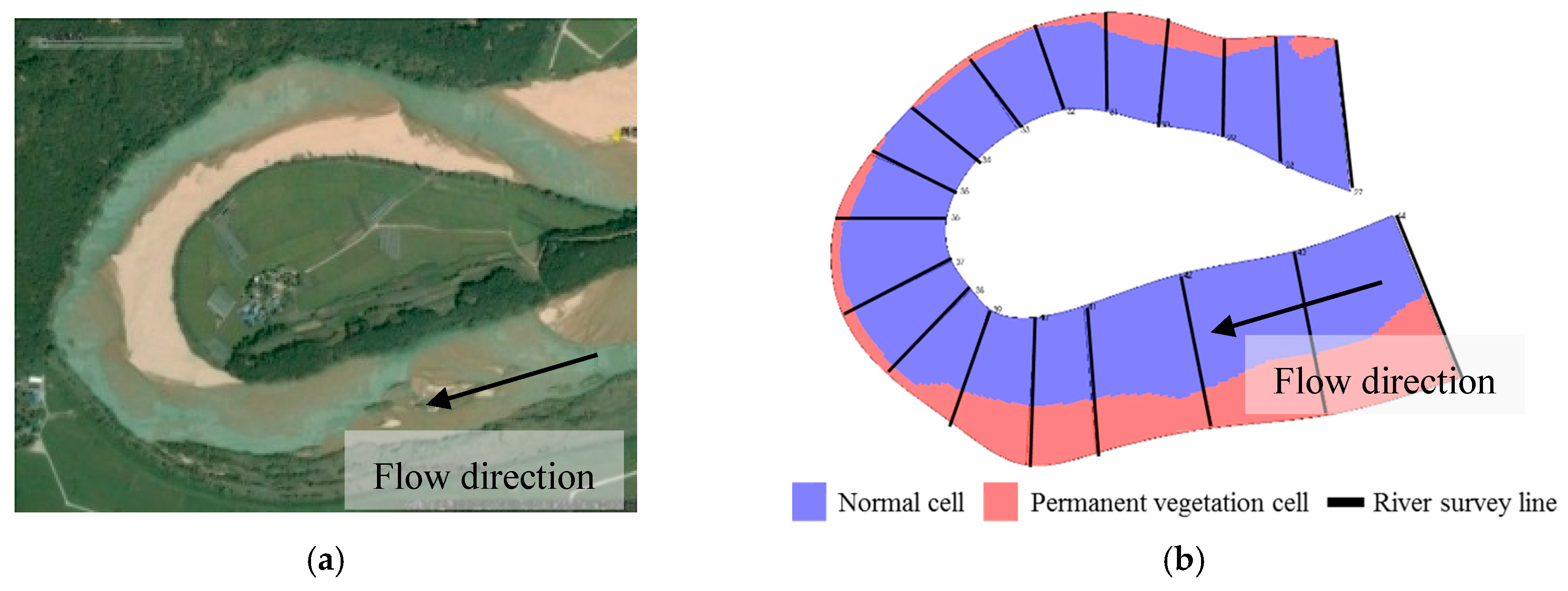
The subject region of the present study is the Hoeryongpo, at the meander of the Nakdong river, Korea (Figure 1). Many researchers have shown interest in this area because of its diverse hydraulic geomorphic topography, which includes meandering channels, point bars, braided channels, and alternate bars. In particular, this area has a significantly developed point bar with a length of approximately 1 km, due to the sandy nature of the river bed. Owing to this variety of geomorphic features, this area is tremendously valuable as a subject of scientific research.
However, the Hoeryongpo meander is currently facing significant environmental changes due to shifts in flood patterns and a decrease in settlement caused because of the completion of the Yeong-ju Dam in 2016 approximately 40 km upstream of the meander. Moreover, the vegetated area has continually increased since 2009 due to severe drought, and these phenomena may result in significant changes to the bed and continue to expand the area of vegetation. If stable vegetation conditions continue to change sediment flow, accelerated by the sediment and flow reduction effects of the dam, the unique topographies present in the Hoeryongpo meander may be totally deformed and eventually disappear.
When facing these hydraulic issues, it is critical that the future effects of flood discharge and vegetation on changes in the river bed should be understood. Hence, this study investigated the effect of vegetation on river bed morphology. In particular, the growth and decay lifecycle of vegetation was quantified to account for non-uniform colonization depending on the water flow patterns. A two-dimensional numerical solver, Nays2DH [37] from iRIC software [38], was used to calculate the water flow, and three different peak discharges, namely, moderate flood level, annual average maximum flood level, and extreme flood level (hereafter called moderate flood, annual average maximum flood and extreme flood or MF AMF and EF, respectively) were evaluated to analyze the interaction between bed morphology and growing vegetation depending on the degree of the river discharge.
2. Material and Methods
2.1. Computational Conditions
The total length of the computational domain was set at 2376 m, the average channel width in this domain was 252 m, and the average bed slope was 0.0015. The Manning roughness coefficient was estimated as 0.016 s/m1/3 from the average sediment diameter (dm) of 1.49 mm, determined using the Manning-Strickler formula.
We used trial and error to obtain a suitable grid size. The shape of the grid was not rectangular because we adopted a curvilinear grid. The average length of the grid cell edges in the streamwise and lateral directions were 8 m and 5 m, respectively. We found that the simulation results obtained using the present grid resolution, such as flow patterns and bed changes, were almost identical to the results obtained using a finer grid resolution (mean sizes of cell edges were 4 m and 2.5 m in streamwise direction and lateral direction, respectively).
This study used three types of coordinate systems: (1) Cartesian coordinate, also called the x-y coordinates (used in the input data: topography and boundary condition, and bed relief index), (2) generalized curvilinear coordinate, also called the - coordinate ( and axes fit to the grid lines), and (3) local streamline coordinates, also called the s-n coordinate (where s is streamline direction of the depth-averaged flow, and n is perpendicular to the s-axis). The computational time step was changeable by the Courant–Friedrich–Lewy (CFL) condition for reducing the CPU time [40].
The effect of vegetation was evaluated as a drag force on the momentum equations. The Ashida and Michiue’s model [41] was used to estimate the bedload flux, and a bed collapse model that considered the angle of repose was incorporated [42]. In addition, at the upstream boundary condition, the inlet velocity at each grid cell was locally calculated using the uniform flow equation based on the Manning formula, taking the bed profile and the local water depth into consideration. In detail, dummy boundary cells were provided outside the upstream end of the computational domain to set inlet boundary conditions. In addition, then the provisional flow velocities at the dummy boundary cells were calculated by the Manning formula. The slope for the Manning formula was assumed to be the average bed slope of the computational domain. Then, the provisional inflow discharge was calculated. The velocity was corrected by multiplying the provisional flow velocity by the ratio of the set discharge to the provisional discharge. Note that the transverse flow velocity at upstream boundary was always set zero. For the downstream boundary conditions, the water level was calculated through the Manning formula and gradient of the velocity component in the streamwise direction was set zero.
Table 1 presents the model parameters for computational condition. Each parameter is explained in subsequent sections.
2.1.1. Hydrodynamic Model
This study used the Nays2DH [37] solver from iRIC. The Nays2DH solver employs the third order total variation diminishing-Monotonic upstream centered scheme for conservation laws (TVD-MUSCL) to solve the advection term and the central scheme for the Reynolds stress term, and a zero-equation type turbulence model based on the shallow flow equations was used.
This model relies on the depth-averaged momentum and continuity equations to calculate plane two-dimensional flow in a generalized curvilinear coordinate. Details of the derivations of the formula are explained in the manual of Nays2DH [37].
2.1.2. Vegetation Model
The vegetation model has been developed by many researchers [6,11,37,43] and it is mostly handles vegetation effect and bed morphology [6,11,43,44]. In the Hoeryongpo meander, the reed (Phragmites), shown in Figure 2a, is the dominant species of the vegetation. The reed is a perennial plant with a primary growing time of approximately 3 months (Figure 2c,d) [45]. Using Figure 2c, we calculated the average growth length as 2.38 m. Its root length is usually 80 cm according to measurement data in this field. As the current study considered only the flood event season, the average germination time of 6 days was neglected. In addition, vegetation shape was assumed to be a rigid cylinder, such that the drag coefficient of vegetation CD was set to 0.7.
The vegetation growth increases the drag force on the channel flow. It inherently hebetates bed erosion and captures the sediment by reducing the flow velocity on the vegetation area; however, bed erosion around the vegetation area is activated by increasing the flow velocity [4,7,9,26]. In addition, roots of vegetation stabilize their colony and suppress the motion of sediment by spatial root distribution, which enhances the tensile strength of the soil [15]. However, in the present vegetation model, we assumed that vegetation is never buried and the effects of root in stabilizing the bed and reducing the sediment transport were neglected. Only the effect of the drag force on the flow was considered.
In this study, it is assumed that if the growth stage () is 0, 0% of the total possible vegetation drag force is applied to the flow calculation, indicating no vegetation is present in the cell, and while the growth stage () is 1, 100% of the vegetation drag force is applied to the flow calculation in each grid cell, indicating fully adult vegetation in the cell.
In the river basin, the growth of vegetation can be influenced by diverse factors, such as the duration of daylight, water flow, and temperature. This means that, for the purposes of this study, it is necessary to simplify the growth factor such that it directly relates the vegetation growth to water flow. We assumed that vegetation begins to grow during the flood season (June to August) and we set the simulation time as 450 h. The time of vegetation growth was 3 months, so that we assumed that the growth stage linearly increases and then reaches a value of 0.2 (Figure 2b) at the end of the simulation (450 h/3 month = 0.21). The decay process of the vegetation is assumed to change depending on the change in the river bed elevation with respect to the root length. As the length of a reed root is approximately 0.8 m (root growth is neglected), it was assumed that a river bed erosion more than 0.8 m eliminates the vegetation in that area, after which the growth stage () becomes 0.
The effect of vegetation density on the drag force of the channel was also considered. In this relationship, the vegetation density is defined as the area of flow interception by vegetation per unit volume (, which is assigned to each computational cell as given by Equation (1) [43]:
where, is the number of vegetation in the unit area, is the average diameter of stalks or trunks, and is the sampling grid width ( is 1 m in this study). According to the KICT [46] report, the average number (/) of overall vegetation in this study area in July is 95.34 EA/m2. Moreover, since the subject vegetation consists primarily of reeds, was assumed to be a small value of 0.01 m. As a result, the value of in the study area was estimated as 1 m−1.
In all simulations, two types of vegetation were used: a permanent type and a non-uniform growth type. The permanent vegetation area (shown in Figure 3b) was assumed as such because this vegetation area had been strongly established along the river bank for more than 10 years (see Figure 3a). Even after annual flood events, the vegetation in this area remained. Therefore, this vegetation area can be regarded as one of the constant factors of the topography. If vegetation in this area is neglected in the simulation, the main flow channel grows wider, the flow velocity shifts into a different phase, and the point bar fails to develop.
The non-uniform growth type of vegetation was also considered. This type of vegetation can grow non-uniformly depending on the water depth in its computational grid. If the water depth is greater than 0.1 m, the growth of vegetation is suspended. If the water depth again becomes smaller than 0.1 m, the growth of vegetation restarts from the current growth stage.
We used trial and error to adjust the initial condition of permanent vegetation. This study area has large point bar, which is main location for vegetation colonization, thus, it is important to reproduce this point bar for present study. Therefore, we considered four Cases to place the permanent vegetation area: around expected point bar area (Case 1), near the inner bank (Case 2), absent of permanent vegetation (Case 3) and near the outer bank and flood plain (Case 4). Case 1 can generate the point bar, but it is too artificial. Case 2 and Case 3 can generate the point bar near the inner bank, but another point bar is generated near the outer bank as much as point bar near the inner bank, so these Cases are inadequate to reproduce the survey data. Case 4 can generate the point bar well, thus, we employed its permanent vegetation area.
The initial growth stage () of permanent vegetation was determined to be 1, and its growth stage does not change. The initial growth stage of non-uniform vegetation growth () was 0, and its growth stage increases depending on the simulation time.
2.1.3. Non-Equilibrium Secondary Flow Model for Sediment Transport of Bed Load
In a curved channel, it is important to consider the sediment transport in the lateral direction because this secondary flow of the first kind is dominant due to the unbalanced pressure in the lateral direction induced by the centrifugal force. In general, the velocity near the bed is evaluated using the Engelund model [47], and the direction of bedload transport is estimated using a secondary flow equilibrium model with Hasegawa’s equation [42]. However, this equilibrium model does not consider the lag between the streamline curvature and the development of the secondary flow.
On the other hand, a non-equilibrium model [48,49,50,51,52] can consider the lag between the secondary flow and the streamline curvature. The transport of the depth-averaged vorticity in the streamwise direction is calculated using the vorticity transport equation, which is associated with the secondary flow of the first kind. The equilibrium secondary flow model only considers the presence of secondary flow, whose strength is in proportion to the streamline curvature, neglecting the development and decay processes of the secondary flow due to change in the curvature of the streamline. The non-equilibrium model can consider the presence of lag, which means delay in the adjustment of the secondary flow to change in the streamline curvature. Hence, results obtained using the equilibrium and non-equilibrium secondary flow models exhibit different tendencies, especially in a sharp meandering channel such as this study area. Therefore, we employed a non-equilibrium model.
2.1.4. Sediment Transport Model
To calculate the bed level change and the sediment transport of the bedload considering non-equilibrium secondary flow model, we used the Ashida and Michiue formula [41] and the Exner equation to calculate the critical Shields number (=0.0374 in this study area), and we used the Iwagaki equation [53] to calculate the Shields number .
2.1.5. Slope Failure Model
A slope failure model was employed in this study, which is consistent with several existing research studies (e.g., [6,11,54,55]). In the present model, slope failure was considered at each two adjacent grid cells. If the bed slope at two adjacent cells exceed the angle of repose, sand from the higher cell is moved to the lower cell to satisfy the slope, just as the angle of repose. This adjustment is applied at the entire computational domain. This sweep is repeated until all bed slopes at the two adjacent cells become smaller than the angle of repose. In this process, the total volume of bed material is conserved. In this study, the angle of repose is 30° because almost the entire riverbed consists of sand, which has an angle of repose ( of approximately 30°.
2.1.6. Hydrograph Characteristic Shape
To account for the diverse conditions of a flood event, a hydrograph characteristic shape, which can reflect a typical hydrograph for this location, is required. The observed river discharge data consists of several types of hydrographs, such as annual average maximum flood discharge, extremely big discharge, and moderate scale flood discharge. It is, therefore, difficult to select a typical hydrograph among such diverse observation data. Moreover, we were unable to clarify the starting time and ending time in each flood event because the flood event can consecutively occur during the flood season. Thus, a simplified hydrograph characteristic shape can be assumed to evaluate the growing vegetation effect under the same hydrograph shape.
The process of generating the hydrograph characteristic shape is as follows:
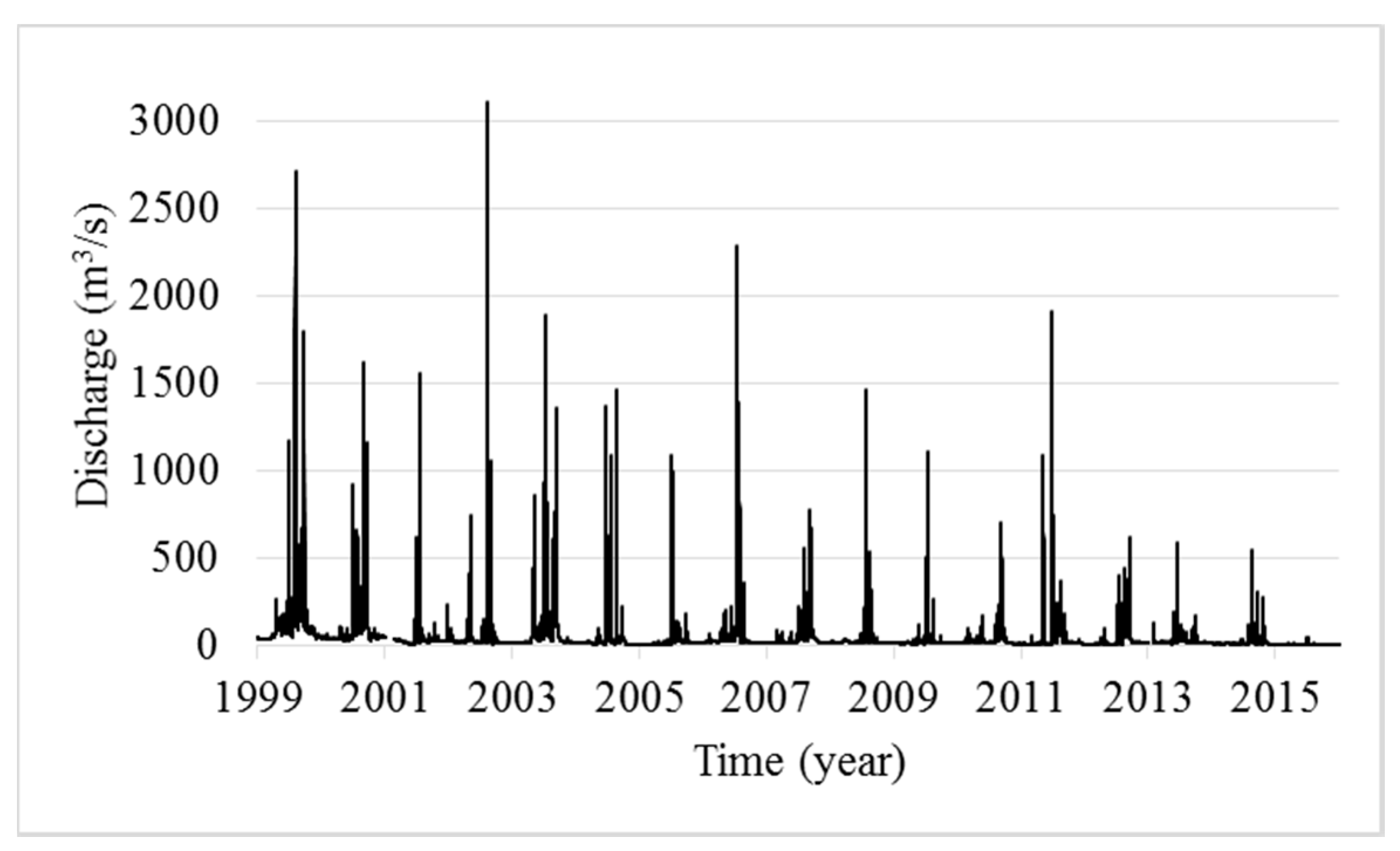
- Flood events, with the annual maximum peak, were selected from 15 years of measurement data (see Figure 4), except for the 2015, as the hydrograph for this year shows less than half of the annual averaged maximum discharge (690 m3/s) of the other years. Thus, a total of 14 hydrographs were extracted from 15 years’ data;
- Each hydrograph was normalized using each peak discharge and then trimmed at the inflection points;
- And then, the hydrograph characteristic shape was calculated by ensemble averaging with all of 14 normalized hydrographs. Before taking ensemble averaging, the start times of all hydrographs were adjusted so that the times to peaks become the same. We also assumed that the discharge at the start and the end of the hydrograph is the total averaged discharge for 15 years. As a result, the flood duration of the hydrograph characteristic shape becomes 150 h.
Using this hydrograph characteristic shape, hydrographs with arbitral peak discharges can be obtained easily through calculation (hydrograph characteristic shape × peak discharge) as shown in Figure 5.
We should check whether the created hydrograph with the hydrograph characteristic shape reproduces real hydrographs or not. In Figure 5, the shape of the created and observed hydrographs are compared. As shown in Figure 5, calculated hydrograph (Cal.) has a similar shape as the measured hydrograph (Obs.). Moreover, the mean value of the correlation coefficient (R2) between the calculated data and the observed data was estimated as 0.9505. Therefore, the hydrograph characteristic shape is useful to create a typical shaped hydrograph with arbitrary peak discharges in the study location.
To reflect the relationship between non-uniform vegetation growth and peak discharge, this study considered three discharge levels: MF (Moderate Flood) season (peak discharge: 690 m3/s), AMF (Annual average Maximum Flood) season (peak discharge: 1381 m3/s), and EF (Extreme Flood) season (peak discharge: 2762 m3/s). The AMF is the annually averaged maximum peak discharge of the study area, the MF season is assumed to have half the peak discharge of AMF season, and the EF season is assumed to have twice the peak discharge of AMF season. Note that all the three general discharge magnitudes have been observed in the study area. In addition, all the durations of the flood events are unified into the duration of the normal case (150 h per one flood event) to consider the same vegetation growth time. Here, each flood event duration is 150 h, which is longer than the observed flood event in Figure 5. However, all observed discharges in Figure 5 start with overlapping on the previous flood event; therefore, the real duration of the flood event is longer or similar to that of the generated hydrograph characteristic shape.
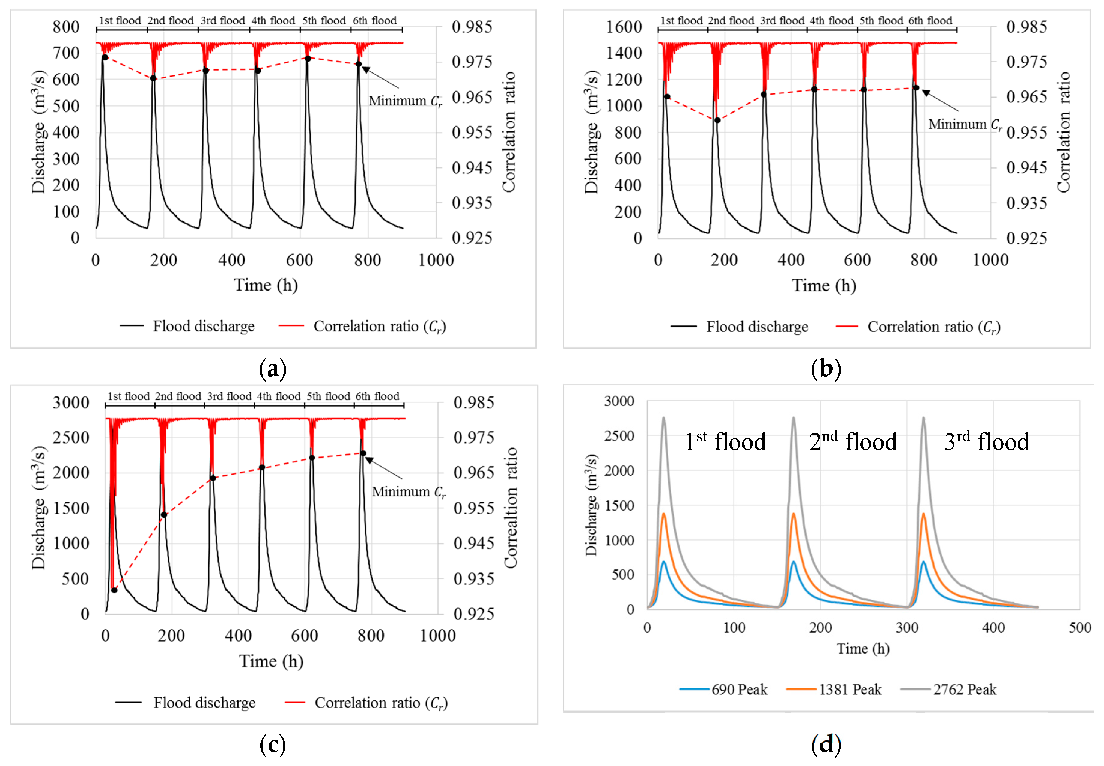
If the simulation is run for the AMF season (peak discharge: 1381 m3/s), the final channel pattern should match the surveyed data (see Section 2.3), because the river bed and topography have been in a state of morphological equilibrium (maintaining a point bar shape in this study) for a long period of time. It is difficult to determine the number of flood events attaining morphological equilibrium. Therefore, in this study, we arbitrarily selected the number of flood events (three times), referring the annual averaged frequency of typhoon (three times/year in Korea) [57]. We tried to check the validity of the number of flood events. For this, we introduced autocorrelation ratio ( of the bed profile between the current bed profile and the previous bed profile (before 6 hours, which is arbitrarily selected, and is enough long to cause bed elevation change and is much shorter than the period of one flood event). The autocorrelation ratio was calculated using Equations (2)–(5) [4] as follows:
where, is the autocorrelation ratio, is the previous bed profile, is the bed elevation (current bed profile), is the cross sectional grid index in the Cartesian coordinate; is the total number of cross sectional grids, is the averaged previous bed elevation in each cross section, and is the averaged current bed elevation at each cross section. If the autocorrelation ratio () reaches 1, the channel is totally stable (no bed changing), while if this ratio reaches to 0, the channel is totally unstable (extreme bed changing) [4,6]. The autocorrelation ratio ( was calculated at every grid cross section at every 1 h. Then, all values of the autocorrelation ratio ( over the entire computational domain were averaged.
Figure 6a–c shows the temporal changes in the autocorrelation ratio ( and Figure 6d shows the hydrograph characteristic shapes with the three different peaks. In Figure 6a–c, the correlation ratio ( becomes minimum when peak discharge occurs. We found that the amplitude of variations of becomes mostly stable after the three flood events. In Figure 6c (EF case), the amplitude is still decreasing after the third flood event, but the slope of change becomes suddenly milder. It indicates that those bed shapes can be assumed to reach the periodically quasi-equilibrium state. The results imply that the hydrograph including three flood events will cause no serious problems to consider the effects of vegetation.
In all, six simulation cases of three flood discharges each were run in this study. The total duration of the flood event was set as 450 h in all simulation cases. Non-uniform vegetation growth and permanent vegetation growth were considered for each discharge case, as presented in Table 2.
2.2. Verification of Simulation
When conducting the simulation, the flat-bed state was set as the initial bed, which has a constant slope (0.0015). This is because this study investigated the responses of bed morphology on growing vegetation effect by comparing several cases (e.g., change in the peak discharge and the presence of vegetation growth effect). To consider the vegetation growth time, the duration of the flood event should be limited and unified, so that we employed the hydrograph characteristic shape (duration is 450 h).
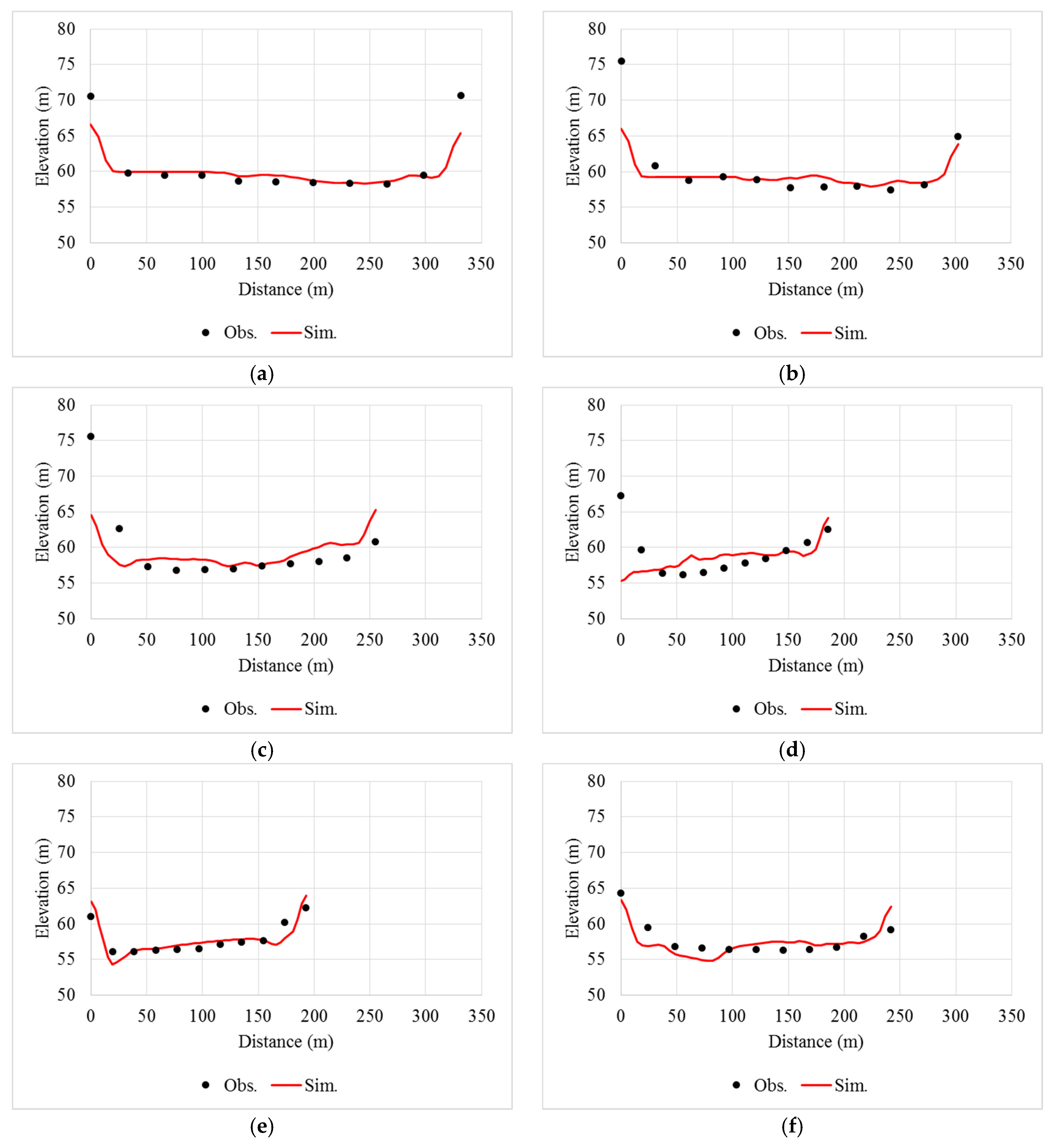
The final simulated channel shape was compared with observed data to verify the model. For these simulation results, a standard hydrograph (see Figure 3) with peak discharge of a 1381 m3/s was used. The verification case did not consider the growing vegetation in order to reflect the environment of the present study area. Figure 7 shows the simulated and observed bed elevation of the grid cross sections (the end of the downstream grid is at i = 319). The number of measurement points was 11. Figure 7a,b show a comparison of the observed and simulated cross sections located at a part of the inlet straight channel. Figure 7c–f shows the observed and simulated bed elevations along grid cross sections at the meandering part. The bed elevation near the inner bank is higher than that near the outer bank, because point bar is developed near the inner bank. Moreover, secondary flow of the first kind occurs and erodes the river bed near the outer bank during flood event such that the bed elevation near the outer bank is lower.
Figure 7d shows that the outer bank totally collapsed because this model used the slope failure model (Section 2.1.5) and the angle of repose was 30. Thus, if the river bed adjacent to the bank is highly eroded, the bank elevation (initially rectangular in this study) can be decreased [11] or the meander amplification is activated. In this study, the river is surrounded by artificial bank and mountain, such that the bank failure does not occur; however, this model cannot consider such bank profile.
The differences of bed elevation between simulation result and observation data are 2–3 m, which may come from some of uncertainties, such as, irregularities on non-uniform grain size, permanent vegetation area and surveyed topography. Nevertheless, the simulated channel profile shows a similar pattern with the observed channel profile. Moreover, averaged correlation coefficient (R2) between channel profiles in the simulation and observation was 0.63. These results show the adequacy of the present computational setup.
2.3. Channel Pattern Quantification
2.3.1. Braiding Index
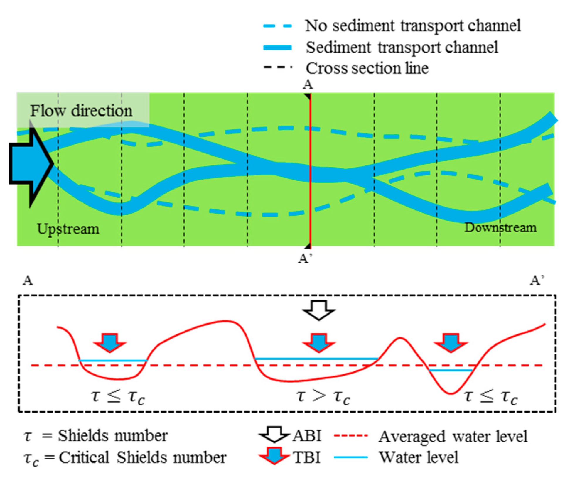
The braiding index is a useful indicator for evaluating the magnitude of channel braiding. This index has been studied using two different methods [58]. One method considers the total sinuosity, while the other method considers the channel count. In this study, the channel count method proposed by Bertoldi, et al. [59] was used as it calculates the braiding index simply and intuitively. This method employs the total braiding index (TBI) and the active braiding index (ABI). Essentially, the TBI counts the total number of channels at each cross section as shown in Figure 8, while the ABI counts only the active channels (channels with a Shields number larger than the critical Shields number). Compared with the ABI, the use of the TBI is insufficient to explain the state of spatial sediment transport. Therefore, this study uses the ABI to quantify changes in the channel pattern. If the ABI is large, the river has many thread channels, while if the ABI is small, the river has few channels; a river with an ABI of 1 has only an active single channel.
The cross sections are well defined in 1-D modelling. However, they are not clear for 2-D modelling because it is difficult to clarify the main flow direction. Thus, we considered the grid cross section based on river survey data (Figure 3b) to evaluate the ABI and the BRI.
2.3.2. Bed Relief Index
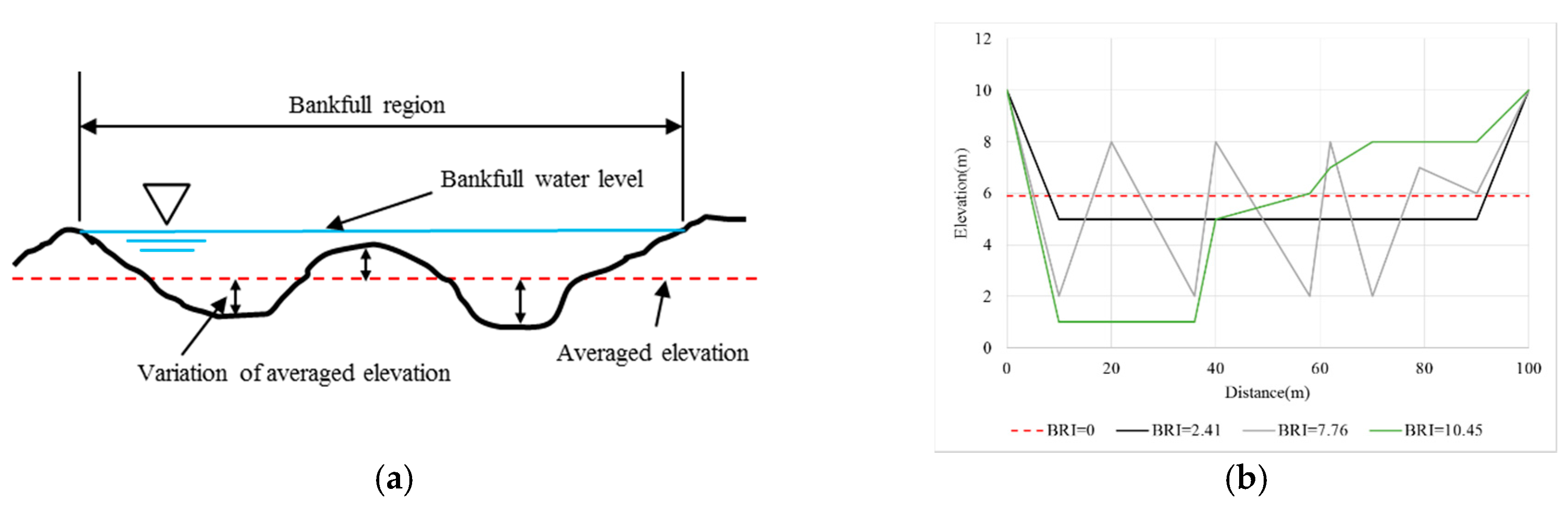
The bed relief index (BRI) [60] indicates the magnitude of relief for a river bed. It can be used to evaluate the amount of bed variation and the flatness of the bed level (Figure 9a). In particular, this index the relative depth of the thalweg in consideration of each mean value of the cross-sectional bed elevation: the BRI increases as the thalweg depth increases. The BRI is calculated using Equation (6):
where, is cross-sectional grid point at (y direction) in the Cartesian coordinate, is the distance between grid points and (m), and is the elevation at .
Figure 9b shows cross sections for different BRI values. At the same average elevation, if the BRI is 0, the channel has a totally flat-bed; as the BRI increases, the channel has a more uneven bed.
3. Results and Discussion
3.1. Local Erosion and Global Erosion
In a curved channel, the cross-stream velocity is an important factor influencing the main flow pattern. Cross-stream velocity notably increases the strength of the secondary flow of the first kind, changing the shear stresses and resulting in a diverse pattern of erosion depth [36]. Eventually, this pattern influences the growth of vegetation and subsequently the changes in bed morphology.
In this study, two types of erosion are defined: Local erosion and global erosion. Local erosion is caused by increased flow velocity near areas of vegetation [61], as shown in Figure 10a. This local erosion often increases in several channel threads when water level is lower as a flood event recedes. Global erosion is caused by secondary flow of the first kind during bankfull discharge. If the flow discharge grows large enough and the channel shape is curved, the strength of the secondary flow becomes substantial, as shown in Figure 10b.
These two types of erosion result in different bed changes. Local erosion increases the ABI, because the number of thread channels increases. Global erosion increases the BRI, because it deepens the thalweg. Sometimes, global erosion sweeps away thread channels, decreasing the ABI. The dynamics of local and global erosion are described in detail through the formation of bar and thalweg features in the next section.
3.2. Final Channel Patterns and Distribution of Vegetation Area
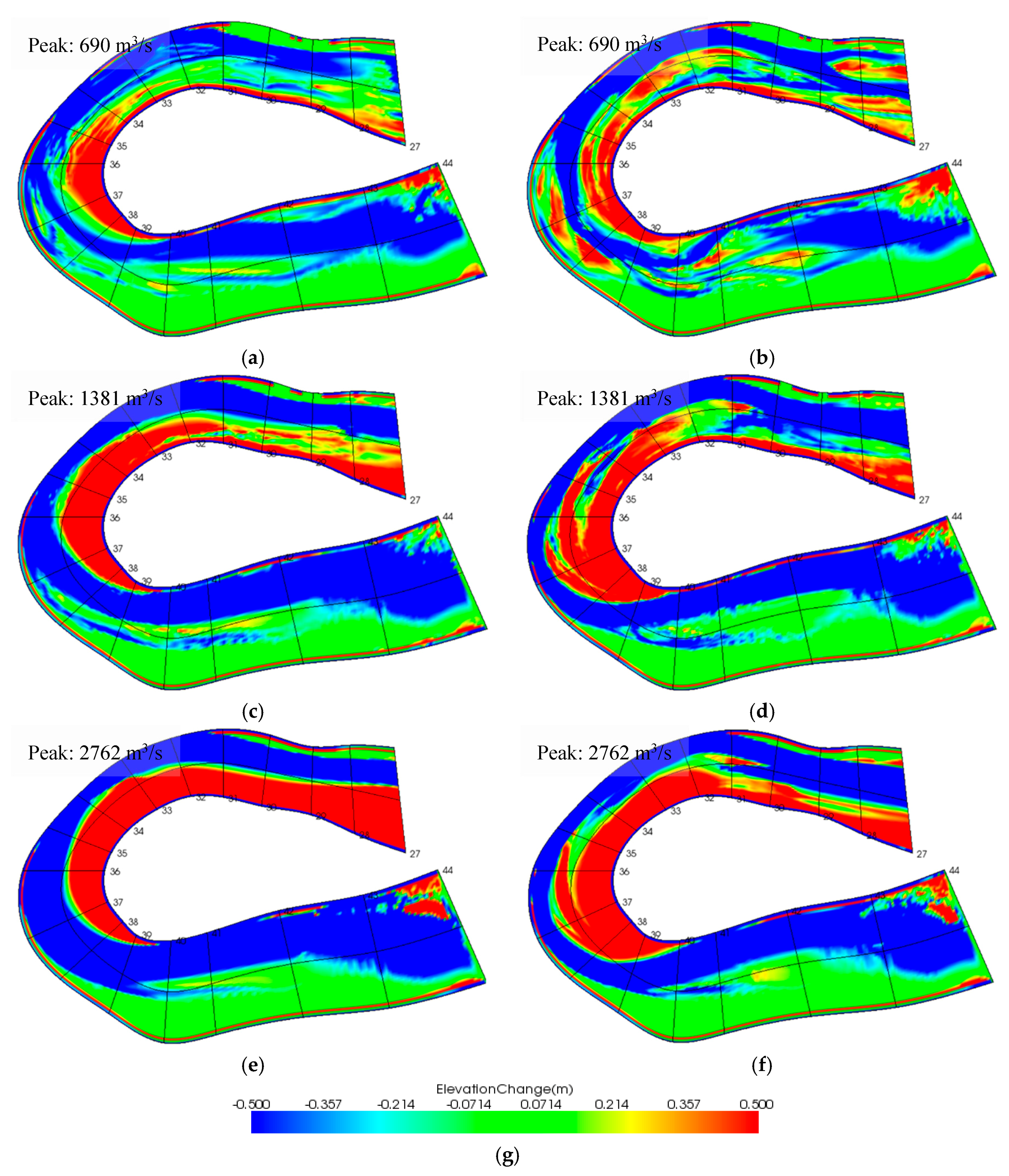
The final channel patterns are shown in Figure 11, which shows the change in the elevation (m) from the initial flat-bed condition, with a constant initial slope of 0.0015. The ranges are limited within ±0.5 m to clearly express the shifting channel patterns. In all cases shown in Figure 11, the point bar is well developed by flood discharge. Note that in these figures, the area just downstream of the inlet maybe affected by the inlet boundary condition. Therefore, the analysis should be carried out in all areas except in this area.
The width of the upper point bar (at the entrance of the meander) increases more for the growing vegetation cases than for the no-growing vegetation cases (for peak discharges of 1381 m3/s and 2762 m3/s). In the cases with no growing vegetation, the point bar near the inner bank migrates downstream as the discharge reaches its peak. However, in the cases with growing vegetation, the growth of vegetation on the point bar reduces the flow velocity and captures more sediment, depositing it near the point bar in the lateral direction.
In cases of small peak discharge (690 m3/s) for the growing vegetation case, the point bar exhibits a smaller width (Figure 11b) than for the same peak discharge under the no-growing vegetation case (Figure 11a). This is due to the reduction in the flow velocity by the growing vegetation, which inhibits the strength of the secondary flow, resulting in a lower flow discharge, which allows vegetation to grow on the outer bank, thus, stabilizing it. As a result, the thalweg does not shift toward the outer bank, instead, it develops along the channel centerline.
Such vegetation colonization (the case of small peak discharge) with bed morphology can be observed in real rivers. Gurnell and Grabowski [14] carried out field survey and reported that the lack of vegetation colonization together with small stream power can cause the settlement of perennial vegetation that develops within the threads river channel. In addition, if vegetation settlement is initiated with small flood discharge during drought season, vegetation colonization may be accelerated. Gurnell et al. [12] carried out field survey and analysis with a conceptual model and proposed that the three phases of gravel bed channel are due to the interaction between bed morphology and vegetation colonization: phase 1 is the initiation of the riparian margin, phase 2 is morphological development of the riparian margin, and phase 3 is full morphohydraulic integration of the riparian zone. Specifically, this study explains the development of the river margins. First, a pool and a riffle were created through the formation of the river margins, which is initiated by sediment deposition with initial vegetation settlement, in newly generated channel (phase 1). Then, the vegetation areas expand their colony, which can influence the development of bar migration and channel alteration in phase 2. If the vegetation colonization is fully expanded, vegetation may overwhelmingly control the change of the river channel (phase 3) in a large time scale.
The phase of the present study area can be estimated as phase 2 (Figure 11c) because vegetation initiates the colonization expansion, although the impact is insufficient to change the bed shape [46]. However, if the flow discharge is consistently small due to the MF season or dam effect, this study area may expand to phase 3 because vegetation colonization expanded after several years as shown in Figure 11b. Figure 1 also shows such phase change from phase 2 to phase 3.
Meanwhile, the cases of normal peak discharge (peak discharge: 1381 m3/s) and extreme peak discharge (peak discharge: 2762 m3/s) may also expand to phase 3; however, it is expected that they exhibit different phases in vegetation colonization and bed changing. These cases may lead to the development of the point bar shape (Figure 11c–f); however, the area of the point bar may slightly increase due to expanded vegetation colonization. Therefore, it is predicted that vegetation colonization stabilizes this study area from bed changing in phase 3.
Figure 12 illustrates the predicted distribution of vegetation in the study area, showing vegetation growth stage by color. If the growth stage is 0 (blue color), the area has no vegetation because vegetation is unable to grow at a water depth higher than 0.1m (germination depth) or it is removed by bed changing (depth of erosion > 0.8 m). If the growth stage is 1 (red color), the area is covered with permanent vegetation (see Section 2.1.2). Note that the maximum growth stage for growing vegetation is 0.21. In these results, the permanent vegetation area plays an important role in generating the bar and thalweg. Because the flow velocity increases near the permanent vegetation area as it does the near a growing vegetation area, local erosion occurs by chute cutoff [62]. Figure 12a shows the vegetation areas located on both sides of the channel because the inundation time is short, and the flow velocity is too small to remove vegetation for the smaller peak discharge (690 m3/s). As a result, the strength of the secondary flow of the first kind is very weak, causing the thalweg to deepen along the centerline. In this case, the local erosion is dominant near the vegetation area, resulting in the development of thread channels.
In cases of larger peak discharge (1381 m3/s and 2762 m3/s) a larger vegetation area develops on the point bar (Figure 12b,c) because the flow velocity causes a strong secondary flow that deepens the thalweg and shifts it toward the outer bank. Therefore, water flow is easily concentrated along the thalweg, and the area of the unsubmerged point bar increases, concurrently increasing the vegetation area more than for the smaller peak discharge case (690 m3/s).
3.3. Change in the ABI and BRI over Time
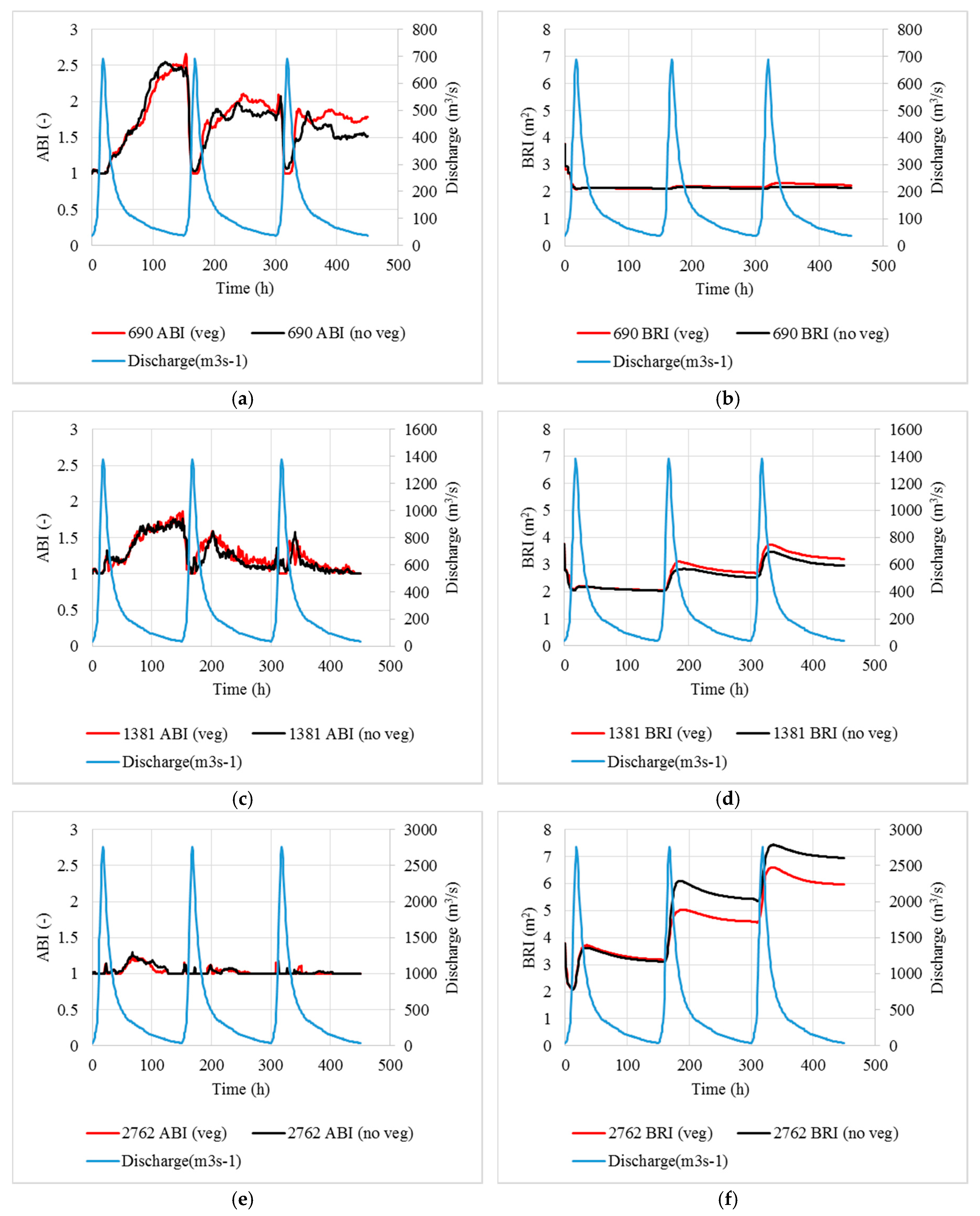
The change in the ABI and BRI were calculated with respect to the time step in order to compare the quantified bed changes. If the ABI increases, several thread channels or islands have been generated. If the ABI decreases, the number of thread channels has decreased. If the BRI increases, the thalweg has deepened, and if the BRI decreases, the thalweg has become shallower.
The change in the ABI over time exhibits different patterns depending on the level of the peak discharge (Figure 13). If the peak discharge is low, the maximum ABI increases because global erosion is weak. Instead, chute cutoff becomes active, and, in the case of growing vegetation, the flow velocity increases near the growing vegetation and causes local erosion. This, in turn, causes channel threading. As a result, for a small peak discharge, the change in ABI over time is larger for the growing vegetation case than for the no-growing vegetation case.
When the flood discharge is extreme (2762 m3/s), the maximum ABI decreases (Figure 13e) because all channels have been inundated by the high flood discharge, which raises the water level. Furthermore, global scale erosion caused by a strong secondary flow of the first kind results in a decrease in the ABI.
The change in the BRI over time also exhibits different patterns depending on the peak discharge for the growing vegetation case. When the peak discharge is low (690 m3/s), the change in the BRI over time decreases; when the peak discharge is high, the change in the BRI over time increases (Figure 13b,d,f). In particular, a high discharge through a meandering channel may cause water flow to concentrate along the thalweg, which then shifts to the outer bank due to the secondary flow of the first kind. This results in a deepening of the thalweg, followed by an increase in the BRI.
Clearly, the ABI and BRI are altered by the effects of vegetation for different degrees of flow discharge. For a small discharge (690 m3/s), the vegetation acts to accelerate local erosion [11,61,63], which increases the ABI. Similarly, if the peak discharge is low (690 m3/s), the BRI increases slightly over time due to local erosion of the vegetation area, whereas if the peak discharge is high (1381 m3/s), the BRI increases significantly for the higher discharge and vegetation effects, which accelerates both local and global erosion.
However, if the peak discharge is extreme (2762 m3/s), the change in the BRI over time is less than for the no-growing vegetation case because the larger vegetation area limits the scale of the secondary flow of the first kind, resulting in global erosion within unvegetated areas, such as the thalweg [36]. Therefore, the maximum depth of erosion increases along the thalweg, but the depth of the thalweg remains shallower than for the no-growing case.
3.4. Bar and Thalweg Dynamics under Different Levels of Flood Discharge: First Flood Event
For each vegetation simulation case, three consecutive occurrences of one of three flood magnitudes were evaluated. This section describes the bar and thalweg dynamics under the occurrence of the first flood event.
During the rapidly increasing flow stage approaching peak discharge, the riverbed begins to actively erode due to the increasing flow velocity and water level. An alternating bar then rapidly develops and migrates downstream. When the flood discharge reaches its peak, the entire computational domain is inundated by water flow. At this time, the ABI decreases to 1 (indicating the presence of a single channel), and the BRI increases (Figure 13).
Under these conditions, the effects on the outer bank are dominated by erosion due to the secondary flow of the first kind. While the inner bank also faces erosion, it is relatively less severe. As a result, the water flow sweeps away the alternating bar near the outer bank, and the alternative bar near the inner bank migrates downstream where it changes into a point bar.
If the peak discharge is extreme (2762 m3/s), the inundation time is longer, the secondary flow grows larger, and global erosion is dominant in the entire study area. At this time, a deeper thalweg develops, causing the BRI to dramatically increase (Figure 13). However, the ABI collapses to 1 because the entire channel is submerged by the water flow (Figure 13e).
As the flood recedes, the water level gradually decreases, and water flow concentrates from the point bar near the inner bank into the thalweg near the outer bank. At same time, a thread channel is generated by chute cutoff [62], and local erosion occurs near the permanent vegetation area, so that the ABI increases and the BRI decreases. If the peak discharge is small (690 m3/s), the thalweg develops along the centerline of the channel because the secondary flow of the first kind is insufficient to erode towards the outer bank.
In the second and final flood events, the river bed responses show partially similar channel patterns to the first flood, but the area of the point bar and thalweg are more developed, eventually initiating shape maintenance (Figure 11a,c,e). In particular, Figure 13c indirectly shows the developing process of thalweg through the changes in ABI. At the tail of the first flood, thalweg and chute cutoff are actively developed in the first flood, thus ABI increases. In addition, then, the thalweg moves and expands towards near the outer bank in second and third floods, thus, the thread channels by chute cutoff is engulfed in thalweg. Therefore, ABI decreases in the tail of second and third floods.
3.5. The Effect of Vegetation Depending on the Peak Discharge: Second and Third Flood Event
During the occurrence of the first of three floods, the cases under the effects of growing vegetation show similar patterns to the cases under no growing vegetation (Section 3.4). The changes in ABI and BRI over time also show similar patterns (Figure 13), because the effect of growing vegetation is not initially strong. However, after the first flood event, the vegetation effect grows stronger and the bed change displays a different pattern as the vegetation begins to grow.
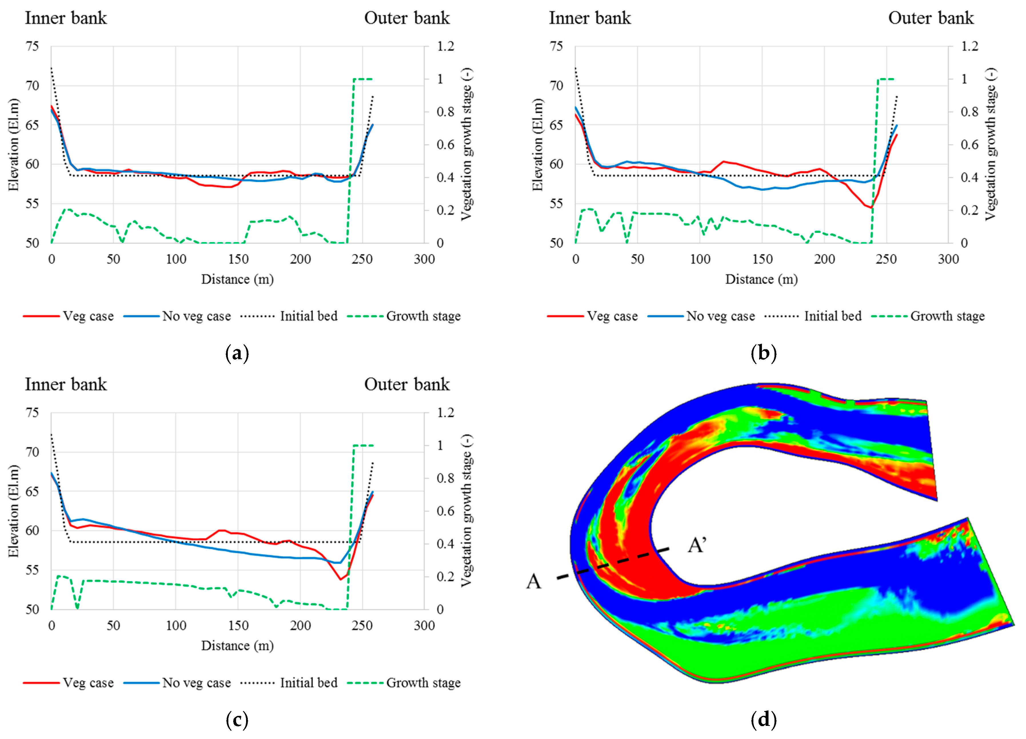
Figure 14 shows the final cross-sectional elevation of the midstream channel (Figure 14d). In this Figure, ”veg case” indicates the growing vegetation case and “no veg” indicates the no-growing vegetation case. Under growing vegetation case, “Veg growth stage” indicates the growth stage of the vegetation rate depending on the given location in the cross-sectional direction. If “Veg growth stage” is 1, the area exhibits permanent vegetation, which is typically located on the outer bank, if the rate is less than 1 and greater than 0, the area exhibits growing vegetation, and if the growth stage is 0, the area is unvegetated. However, “Veg growth stage” of the no-growing vegetation case only indicates 1 near the outer bank as permanent vegetation, which is same with permanent vegetation under growing vegetation case. Using Figure 14, the depth of the thalweg and degree of erosion can be estimated in relation to the peak discharge.
Under a small degree of peak discharge (690 m3/s) with growing vegetation, the flow velocity increases near the areas of vegetation (containing both permanent and growing vegetation), causing local erosion and increasing the depth of erosion (Figure 14a). This erosion accelerates to generate several thread channels [11,61,63], so that both the BRI and ABI increase over time.
If the peak discharge is larger (1381 m3/s), rather than creating thread channels, the depth of the thalweg increases, and the thalweg shifts toward the outer bank (Figure 14b). Because such a large flood discharge increases the flow velocity, a curved channel, in particular, increases the degree of erosion in the transverse direction due to secondary flow of the first kind. Under this peak discharge with growing vegetation, both local and global erosion is activated by the effects of the vegetation and secondary flow. As a result, the maximum ABI decreases, while the maximum BRI increases more than under the no-growing vegetation cases (Figure 13c,d).
However, if the peak discharge is extreme (2762 m3/s), the effect of the vegetation changes. In this case, global erosion is dominant as the discharge reaches its peak. As a result, the thalweg readily shifts toward the outer bank, so that the unsubmerged area on the point bar increases and the vegetation area expands along the larger point bar. If vegetation expands sufficiently, this area can easily limit the scale of secondary flow [36], because the flow velocity decreases along the vegetation. Therefore, global erosion is activated within the unvegetated areas, such as the thalweg, and the growing vegetation case in Figure 14c shows a shallow thalweg near the outer bank. Consequently, the change in BRI over time is smaller than that of the no-growing vegetation case.
Note that, in Figure 7 at the Section 2.2, we compared the cross-sectional patterns between observation data and simulation data and found that the difference of the two data is 2–3 m, which was expected to be induced by some uncertainties in the field conditions. In Figure 14, we can find same order of difference between two data, however the meaning of the difference is very different from the case in Figure 9 because Figure 14 shows the comparison of two simulation results, which use completely same conditions except vegetation effect. Therefore, we can consider that the difference of two results in Figure 14 clearly indicates the vegetation effect.
3.6. Limitation of Modelling and Suggestions
In the present study, the simulation results have reproduced well the observation data, such as point bar, alternating bar, and vegetation effect. However, these results have some limitations. The simulations were carried out under the initial condition with flat bed, which has a constant slope. Therefore, the results of simulations may show rather conceptual and yield typical patterns in bed morphology depending on the vegetation effect and the hydrograph characteristic shape. The most appropriate way for the verification of model is to use detailed survey data regarding bed topography and vegetation for the initial condition. However, such detailed survey data is presently not available. Thus, it is unavoidable to set initial conditions with some artificial way. We expected that simplest bed shape for the initial condition makes it easy to consider the results. Thus, we use the flat bed for the initial condition. It is desirable to obtain more detailed field survey data for the initial condition in the future research.
In addition, the parameter in the vegetation growth model should be specifically considered. Inherently, this study considered that vegetation growth is characterized by linear increases. This simple approach makes it easier to compare the cases for growing vegetation and no growing vegetation.
Moreover, we only considered the vegetation decay by bed erosion to simplify the vegetation model. The effect of burying vegetation by sediment deposition maybe also important for vegetation decay or change of drag force. However, to consider the burying effect, additional models, such as, the changes of root depth and vegetation height, become necessary. Therefore, the present study only focused on vegetation decay by the bed erosion for simplicity. The necessity of the burying effect and the model of it should be considered in further study.
4. Conclusions
In this study, changes in a sharply curved river channel were simulated under two varying parameters: Peak flood discharge and non-uniform vegetation growth effect. To determine the effect of vegetation growth, the change in the channel patterns were quantified using the ABI and BRI. Using this approach, the present study successfully demonstrated that the effects of vegetation were influenced by the flood discharge. The results give basic and useful information, which is useful for river management and flood mitigation. However, some possibilities for future improvements were also highlighted; for instance, more detailed model validation and calibration for vegetation growth parameters. We plan to address such improvements in our future works.
The summary and limitations of this study are as follows.
- Erosion is classified as either local erosion or global erosion. Local erosion is caused by an increase in the flow velocity near an area of vegetation. This erosion may increase the number of threads in the channel as the flood event recedes. Global erosion is caused by strong secondary flow of the first kind working to erode the entire channel as the discharge reaches its peak. While local erosion increases the ABI due to the increase in thread channels, global erosion increases the BRI due to the increase in the thalweg depth. Sometimes, it was observed that global erosion swept away thread channels, resulting in a decrease in the ABI;
- Under a small peak discharge (690 m3/s), vegetation works to accelerate local erosion because the flow velocity increases near the vegetation area, which increases the change in the ABI and BRI over time. If the peak discharge is high (1381 m3/s), the strength of the secondary flow of the first kind becomes significant, thereby activating global erosion. The vegetation effect also activates local erosion, such that the change in the BRI over time is larger than for the no-growing case for the same discharge;However, if the peak flow discharge is extreme (2762 m3/s), global erosion is dominant. The thalweg readily shifts toward the outer bank and the area of point bar with vegetation expansion. Under this scenario, the larger area of vegetation limits the scale of the secondary flow by reducing the flow velocity, which activates global erosion within the unvegetated areas such as the thalweg. As a result, the change in the BRI over time decreases compared to the no-growing vegetation case. This phenomenon should be further explored with more detailed field observation and experimental data;
- In a river, the growth of vegetation is influenced by many factors, such as the duration of daylight, frequency of flood events, temperature, and soil characteristics. Therefore, the growth stage of vegetation should be simplified to allow for a focus on the interaction between the vegetation and flow discharge. Despite the potential overestimation due to this simplification, the simulated shape of the point bar was reproduced with reasonable accuracy compared to pictures (Figure 1 and Figure 11). However, the linear estimation of vegetation growth used in this study is too monotonous to yield quantitative information for practical river training works. Therefore, to ensure more accurate quantitative predictions, further model refinement is necessary by considering a more detailed river survey data and wider variety of real hydrograph, including flood seasons and drought seasons.
Acknowledgments
We express our sincere thanks to Jang, Chang-Lae at Korea National University of Transportation for providing the field data and fruitful advice. We are also grateful to the Ministry of Science and Technology (MEXT) for providing funding for this research.
Author Contributions
Taeun Kang conceived the overall idea of this research. Taeun Kang and Ichiro Kimura designed the computer simulations; Taeun Kang carried out the computer simulations; Taeun Kang and Ichiro Kimura analyzed the data; Taeun Kang, Ichiro Kimura, and Yasuyuki Shimizu contributed to developing the computational tools; while Taeun Kang wrote the paper.
Conflicts of Interest
The authors declare no conflict of interest.
References
- Williams, G.P.; Wolman, M.G. Downstream Effects of Dams on Alluvial Rivers; United States Government Printing Office: Washington, WA, USA, 1984; pp. 1–83.
- Kaufmann, P.R.; Levine, P.; Robinson, E.G.; Seeliger, C.; Peck, D.V. Quantifying Physical Habitat in Wadeable Streams. EPA/620/R-99/003; U.S. Environmental Protection Agency: Washington, WA, USA, 1999.
- Camporeale, C.; Perucca, E.; Ridolfi, L.; Gurnell, A.M. Modeling the interactions between river morphodynamics and riparian vegetation. Rev. Geophys. 2013, 51, 379–414. [Google Scholar] [CrossRef]
- Gran, K.; Paola, C. Riparian vegetation controls on braided stream dynamics. Water Resour. Res. 2001, 37, 3275–3283. [Google Scholar] [CrossRef]
- Braudrick, C.A.; Dietrich, W.E.; Leverich, G.T.; Sklar, L.S. Experimental evidence for the conditions necessary to sustain meandering in coarse bedded rivers. Proc. Natl. Acad. Sci. USA 2009, 106, 16936–16941. [Google Scholar] [CrossRef] [PubMed]
- Jang, C.; Shimizu, Y. Vegetation effects on the morphological behavior of alluvial channels. J. Hydraul. Res. 2007, 45, 763–772. [Google Scholar] [CrossRef]
- Tal, M.; Paola, C. Effects of vegetation on channel morphodynamics: Results and insights from laboratory experiments. Earth Surf. Process. Landf. 2010, 35, 1014–1028. [Google Scholar] [CrossRef]
- van Dijk, W.M.; Teske, R.; van de Lageweg, W.I.; Kleinhans, M.G. Effects of vegetation distribution on experimental river channel dynamics. Water Resour. Res. 2013, 49, 7558–7574. [Google Scholar] [CrossRef]
- Murray, A.B.; Paola, C. Modelling the effect of vegetation on channel pattern in bedload rivers. Earth Surf. Process. Landf. 2003, 28, 131–143. [Google Scholar] [CrossRef]
- Perucca, E.; Camporeale, C.; Ridolfi, L. Significance of the riparian vegetation dynamics on meandering river morphodynamics. Water Resour. Res. 2007, 43, W03430. [Google Scholar] [CrossRef]
- Iwasaki, T.; Shimizu, Y.; Kimura, I. Numerical simulation of bar and bank erosion in a vegetated floodplain: A case study in the Otofuke River. Adv. Water Resour. 2016, 93, 118–134. [Google Scholar] [CrossRef]
- Gurnell, A.M.; Morrissey, I.P.; Boitsidis, A.J.; Bark, T.; Clifford, N.J.; Petts, G.E.; Thompson, K. Initial adjustments within a new river channel: Interactions between fluvial processes, colonizing vegetation, and bank profile development. Environ. Manag. 2006, 38, 580–596. [Google Scholar] [CrossRef] [PubMed]
- Eekhout, J.P.C.; Fraaije, R.G.A.; Hoitink, A.J.F. Morphodynamic regime change in a reconstructed lowland stream. Earth Surf. Dyn. 2014, 2, 279–293. [Google Scholar] [CrossRef] [Green Version]
- Gurnell, A.M.; Grabowski, R.C. Vegetation–Hydrogeomorphology Interactions in a Low-Energy, Human-Impacted River. River Res. Appl. 2015, 32, 202–215. [Google Scholar] [CrossRef]
- Abernethy, B.; Rutherfurd, I.D. The distribution and strength of riparian tree roots in relation to riverbank reinforcement. Hydrol. Process. 2001, 15, 63–79. [Google Scholar] [CrossRef]
- Bennett, S.J.; Pirim, T.; Barkdoll, B.D. Using simulated emergent vegetation to alter flow direction within a straight experimental channel. J. Geomorphol. 2002, 44, 115–126. [Google Scholar] [CrossRef]
- Hicken, E.J. Vegetation and river channel dynamics. Can. Geographer. 1984, 28, 111–126. [Google Scholar] [CrossRef]
- Smith, D.G. Effect of vegetation on lateral migration of anastomosed channels of a glacier Meltwater river. Geol. Soc. Am. Bull. 1976, 87, 857–860. [Google Scholar] [CrossRef]
- Ikeda, S.; Izumi, N. Width and depth of self-formed straight gravel rivers with bank vegetation. Water Resour. Res. 1990, 26, 2353–2364. [Google Scholar] [CrossRef]
- Millar, R.G.; Qucik, M.C. Effect of bank stability on geometry of gravel rivers. J. Hydraul. Eng. 1993, 119, 1343–1363. [Google Scholar] [CrossRef]
- Huang, H.Q.; Nanson, G.C. Vegetation and channel variation; a case study of four small streams in southeastern Australia. Geomorphology 1997, 18, 237–249. [Google Scholar] [CrossRef]
- Millar, R.G. Influence of bank vegetation, on alluvial channel patterns. Water Resour. Res. 2000, 36, 1109–1118. [Google Scholar] [CrossRef]
- Bertoldi, W.; Drake, N.A.; Gurnell, A.M. Interactions between river flows and colonizing vegetation on a braided river: Exploring spatial and temporal dynamics in riparian vegetation cover using satellite data. Earth Surf. Process. Landf. 2011, 36, 1474–1786. [Google Scholar] [CrossRef]
- Van De Wiel, M.; Darby, S.E. Numerical modelling of bed topography and bankerosion along tree- lined meandering rivers. In Riparian Vegetation and Fluvial Geomorphology; Bennet, S., Simon, A., Eds.; AGU: Washington, WA, USA, 2004. [Google Scholar]
- Wu, W.; Shields, F.D., Jr.; Bennet, S.J.; Wang, S.S.Y. A depth averaged two dimensional model for flow, sediment transport, and bed topography in curved channels with riparian vegetation. Water Resour. Res. 2005, 41, W03015. [Google Scholar] [CrossRef]
- Vargas-Luna, A.; Crosato, A.; Uijttewaal, W. Effects of vegetation on flow and sediment transport: Comparative analyses and validation of predicting models. Earth Surf. Process. Landf. 2015, 40, 157–176. [Google Scholar] [CrossRef]
- Tsujimoto, T. Fluvial processes in streams with vegetation. J. Hydraul. Res. 1999, 37, 789–803. [Google Scholar] [CrossRef]
- Crosato, A.; Saleh, M.S. Numerical study on the effects of floodplain vegetation on river planform style. Earth Surf. Process. Landf. 2011, 36, 711–720. [Google Scholar] [CrossRef]
- Perona, P.; Molnar, P.; Crouzy, B.; Perucca, E.; Jiang, Z.; McLelland, S.; Wüthrich, D.; Edmaier, K.; Francis, R.; Camporeale, C.; et al. Biomass selection by floods and related timescales: Part 1. Experimental observations. Adv. Water Resour. 2012, 39, 85–96. [Google Scholar] [CrossRef]
- Ye, F.; Chen, Q.; Blanckaert, K.; Ma, J. Riparian vegetation dynamics: Insight provided by a process-based model, a statistical model and field data. Ecohydrology 2013, 6, 567–585. [Google Scholar] [CrossRef]
- Everitt, B. Use of the cottonwood in an investigation of the recent history of a floodplain. Am. J. Sci. 1968, 266, 417–439. [Google Scholar] [CrossRef]
- McKenney, R.; Jacobson, R.B.; Wertheimer, R.C. Woody vegetation and channel morphogenesis in low-gradient, gravel-bed streams in the Ozark Plateaus, Missouri and Arkansas. Geomorphology 1995, 13, 175–198. [Google Scholar] [CrossRef]
- Nanson, G.C.; Beach, H.F. Forest succession and sedimentation on a meandering-river floodplain. Northeast British Columbia, Canada. J. Biogeogr. 1977, 4, 229–251. [Google Scholar] [CrossRef]
- Rood, S.B.; Mahoney, J.M. Collapse of riparian poplar forests downstream from dams in western prairies: Probable causes and prospects for mitigation. Environ. Manag. 1990, 14, 451–464. [Google Scholar] [CrossRef]
- Robertson, K.M.; Augspurger, C.K. Geomorphic processes and spatial patterns of primary forest succession on the Bogue Chitto River, USA. J. Ecol. 1999, 87, 1052–1063. [Google Scholar] [CrossRef]
- Garcia, X.-F.; Schnauder, I.; Pusch, M.T. Complex hydromorphology of meanders can support benthic invertebrate diversity in rivers. Hydrobiologia 2012, 685, 49–68. [Google Scholar] [CrossRef]
- Shimizu, Y.; Takebayashi, H.; Inoue, T.; Hamaki, M.; Iwasaki, T.; Nabi, M. Nays2DH Solver Manual. 2014. Available online: http://i-ric.org/en (accessed on 21 February 2018).
- International River Interface Cooperative (iRIC). Available online: http://i-ric.org/en (accessed on 21 February 2018).
- Google Earth. Available online: https://earth.google.com/web/ (accessed on 21 February 2018).
- Courant, R.; Friedrichs, K.; Lewy, H. Über die partiellen differenzengleichungen der mathematischen physik. Mathematische. Annalen. 1928, 100, 32–74. (In German) [Google Scholar] [CrossRef]
- Ashida, K.; Michiue, M. Study on hydraulic friction and bedload transport rate in alluvial streams. Trans. JSCE 1972, 206, 59–69. [Google Scholar]
- Hasegawa, K. Hydraulic Study on Alluvial Meandering Channel Planes and Bedform Topography-Affected Flows; Doctoral Paper; Hokkaido University: Sapporo, Japan, 1985. [Google Scholar]
- Shimizu, Y.; Kobatake, S.; Arafune, T. Numerical study on the flood-flow stage in gravel-bed river with the excessive riverine trees. Annu. J. Hydr. Eng. 2000, 44, 819–824. [Google Scholar] [CrossRef]
- Kim, H.; Kimura, I.; Shimizu, Y. Characteristics of local erosion and deposition with a patch of vegetation. Proc. River Flow 2012 2012, 1, 287–293. [Google Scholar]
- National Wetlands Center. Available online: http://wetlandkorea.blog.me (accessed on 21 February 2018).
- Korea Institute of Construction Technology (KICT). Analysis of Change in River Morphology and Vegetation due to Artificial Structure. Internal Research Project Report. 2015. Available online: http://www.nl.go.kr/nl/ (accessed on 21 February 2018). (In Korean).
- Engelund, F. Flow and bed topography in channel bends. J. Hydraul. Div. 1974, 100, 1631–1648. [Google Scholar]
- Onda, S.; Hosoda, T.; Kimura, I. Refinement of a depth-averaged model in curved channel in generalized curvilinear coordinate system and its verification. Ann. J. Hydrau. Eng. 2006, 50, 769–774. [Google Scholar] [CrossRef]
- Kimura, I.; Hosoda, T.; Onda, S. Fundamental properties of suspended sediment transport in open channel flows with a side cavity. In Proceedings of the RCEM 2007, Enschede, The Netherlands, 17–21 September 2007; Balkema Pblishers: Enschede, The Netherlands, 2007; pp. 1203–1210. [Google Scholar]
- Iwasaki, T.; Shimizu, Y.; Kimura, I. Sensitivity of free bar morphology in rivers to secondary flow modeling: Linear stability analysis and numerical simulation. Adv. Water Resour. 2016, 92, 57–72. [Google Scholar] [CrossRef]
- Hosoda, T.; Nagata, N.; Kimura, I.; Michibata, K.; Iwata, M. A depth averaged model of open channel flows and secondary currents in a generalized curvilinear coordinate system. In Advances in Fluid Modeling & Turbulence Measurements; Ninokata, H., Wada, A., Tanaka, N., Eds.; World Scientific: Singapore, 2001; pp. 63–70. [Google Scholar]
- Kalkwijk, J.P.; De Vriend, H.J. Computational of the flow in shallow river bends. J. Hydraul. Res. 1980, 18, 327–342. [Google Scholar] [CrossRef]
- Iwagaki, Y. Hydrodynamical study on critical tractive force. Trans. Jpn. Soc. Civil. Eng. 1956, 41, 1–21. [Google Scholar] [CrossRef]
- Jang, C.; Shimizu, Y. Numerical simulations of the behavior of alternate bars with different bank strengths. J. Hydraul. Res. 2005, 43, 595–611. [Google Scholar] [CrossRef]
- Iwasaki, T.; Shimizu, Y.; Kimura, I. Numerical simulation on bed evolution and channel migration in rivers. River Flow 2012, 1, 673–679. [Google Scholar]
- Water Resources Management Information System. Ministry of Land, Infrastructure and Transport in Korea. Available online: http://www.wamis.go.kr/ (accessed on 21 February 2018).
- National Typhoon Center, Typhoon White Book (in Korean), 2010. Available online: http://typ.kma.go.kr (accessed on 21 February 2018).
- Egozi, R.; Ashmore, P. Defining and measuring braiding intensity. Earth Surf. Process. Landf. 2008, 33, 2121–2138. [Google Scholar] [CrossRef]
- Bertoldi, W.; Zanoni, L.; Tubino, M. Planform dynamics of braided streams Planform dynamics. Earth Surf. Process. Landf. 2009, 34, 547–557. [Google Scholar] [CrossRef]
- Hoey, T.; Sutherland, A. Channel morphology and bedload pulses in braided rivers: A laboratory study. Earth Surf. Process. Landf. 1991, 16, 447–462. [Google Scholar] [CrossRef]
- Schnauder, I.; Sukhodolov, A.N. Flow in a tightly curving meander bend: Effects of seasonal changes in aquatic macrophyte cover. Earth Surf. Process. Landf. 2012, 37, 1142–1157. [Google Scholar] [CrossRef]
- Ashmore, P. How do gravel-bed rivers braid? Can. J. Earth Sci. 1991, 28, 326–341. [Google Scholar] [CrossRef]
- Wolfert, H.P. Geomorphological Change and River Rehabilitation. Ph.D. Thesis, University Utrecht, Utrecht, The Netherlands, 2001. [Google Scholar]
Figure 1.
Computational domain (dark brown area: vegetation area). [39]. (a) Sep. in 2003 year; (b) Sep. in 2004 year; (c) Feb. in 2005 year; (d) Nov. in 2013 year; (e) Nov. in 2015 year; (f) Apr. in 2016 year.
Figure 1.
Computational domain (dark brown area: vegetation area). [39]. (a) Sep. in 2003 year; (b) Sep. in 2004 year; (c) Feb. in 2005 year; (d) Nov. in 2013 year; (e) Nov. in 2015 year; (f) Apr. in 2016 year.
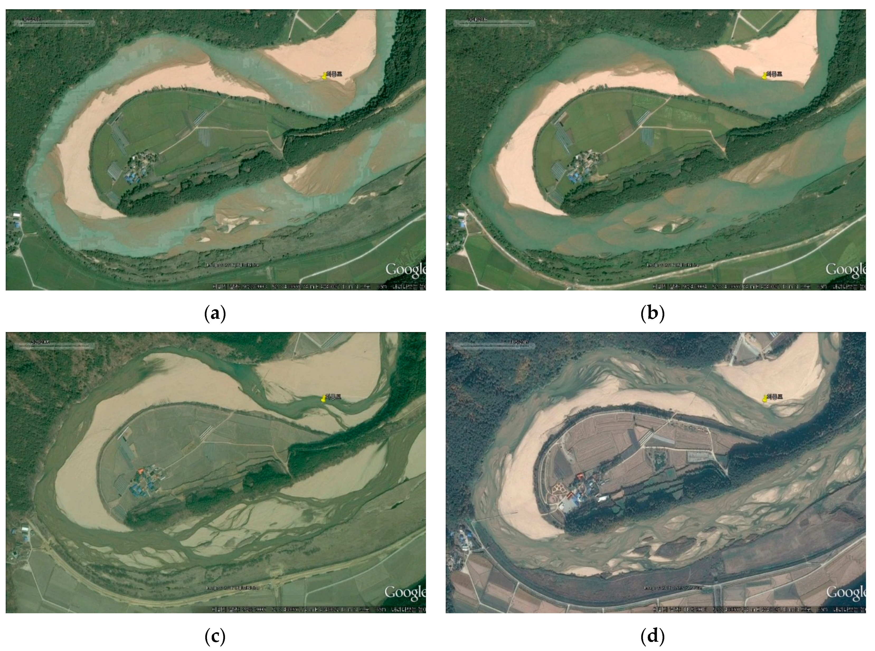
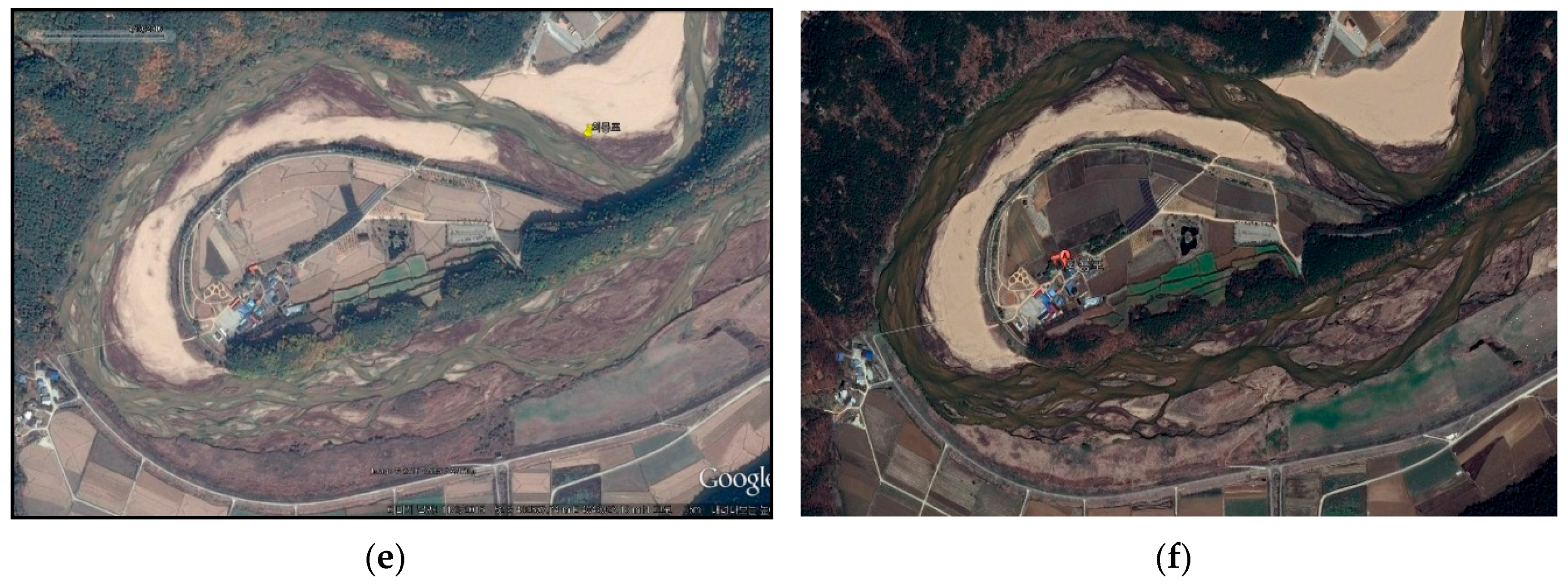
Figure 2.
Vegetation species and growth stage. (a) Sample of reed; (b) growth stage (simulation time: 450h); (c) measured vegetation growth; (d) averaged data from measured data; Sec. is the measured section in Seokchon, Korea [45].
Figure 2.
Vegetation species and growth stage. (a) Sample of reed; (b) growth stage (simulation time: 450h); (c) measured vegetation growth; (d) averaged data from measured data; Sec. is the measured section in Seokchon, Korea [45].
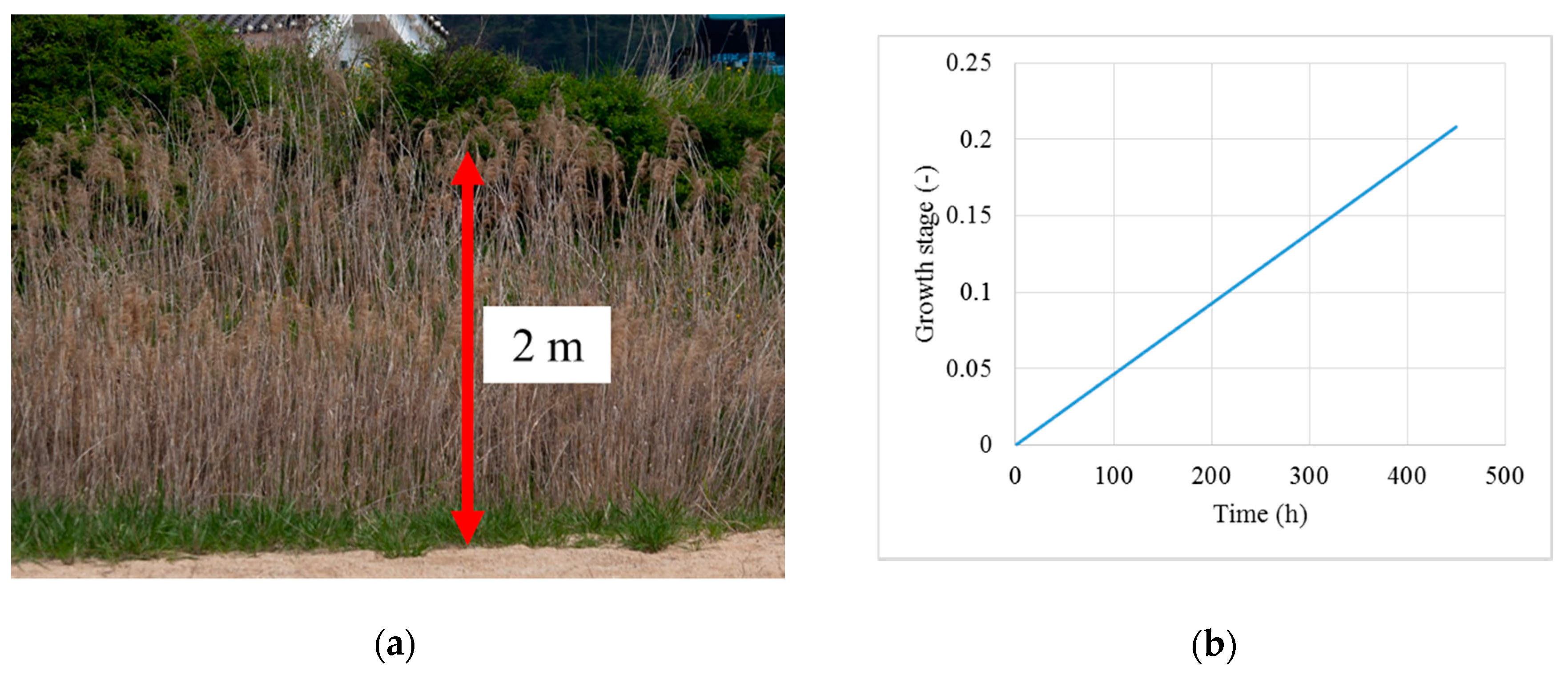
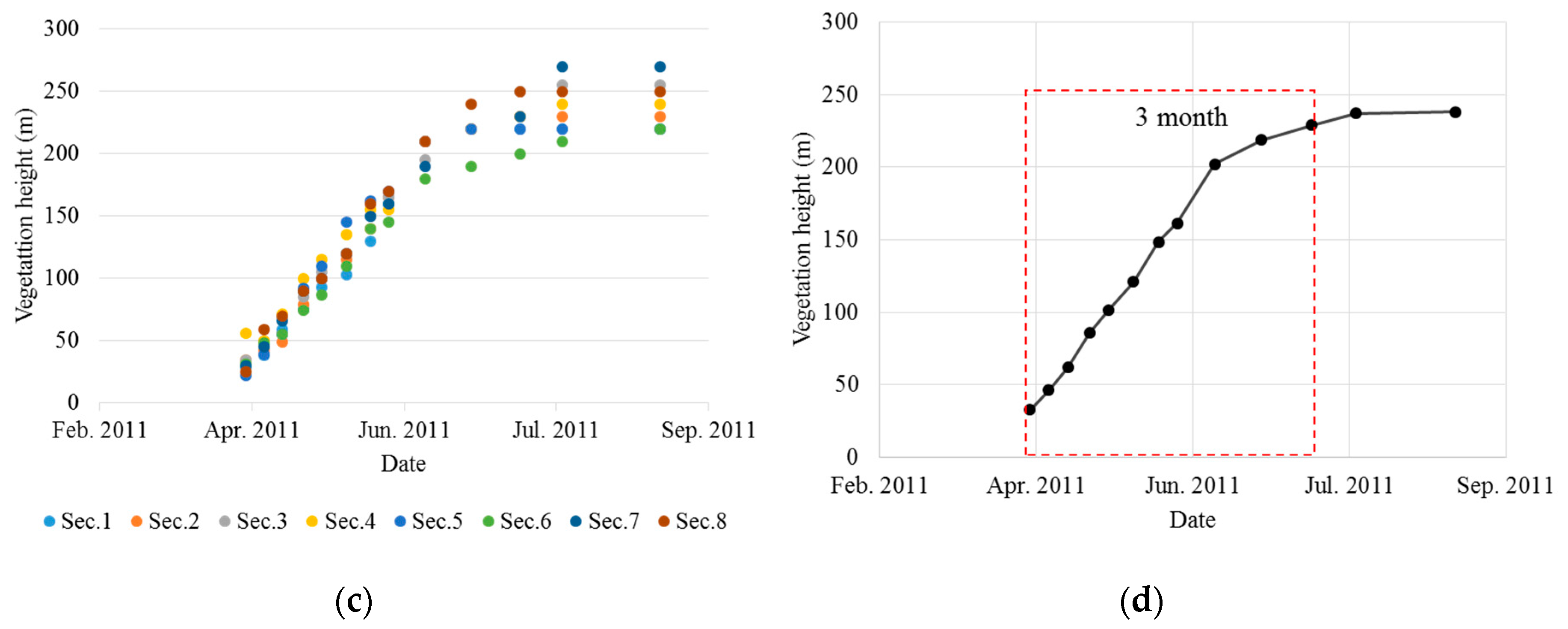
Figure 3.
Permanent vegetation area. (a) study area (2003 year); (b) permanent vegetation area (red color).
Figure 3.
Permanent vegetation area. (a) study area (2003 year); (b) permanent vegetation area (red color).

Figure 4.
Measured discharge [56].
Figure 4.
Measured discharge [56].

Figure 5.
Comparison of observed and calculated flow discharge (Obs: observed discharge; Cal: reproduced discharge using hydrograph characteristic shape with peak discharge). (a) Flood event in 2001; (b) flood event in 2002; (c) flood event in 2006; (d) flood event in 2014.
Figure 5.
Comparison of observed and calculated flow discharge (Obs: observed discharge; Cal: reproduced discharge using hydrograph characteristic shape with peak discharge). (a) Flood event in 2001; (b) flood event in 2002; (c) flood event in 2006; (d) flood event in 2014.
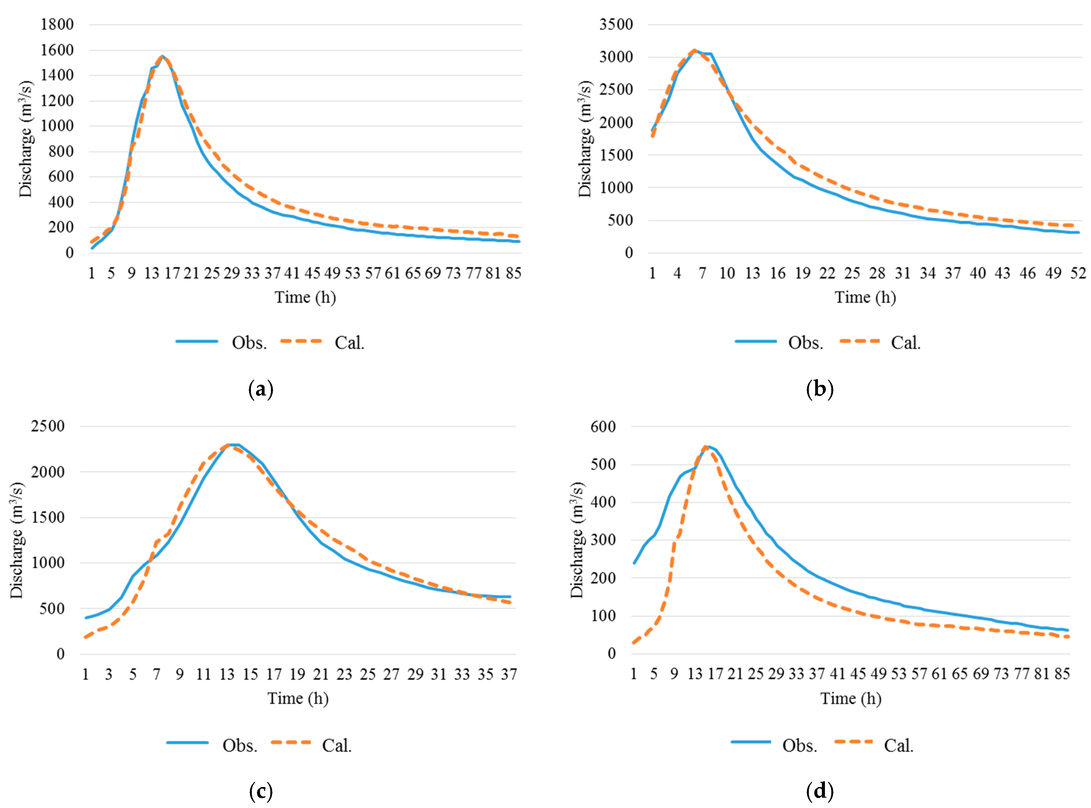
Figure 6.
Hydrograph. (a) correlation of bed changing (peak discharge: 690 m3/s); (b) correlation of bed changing (peak discharge: 1381 m3/s); (c) correlation of bed changing (peak discharge: 2762 m3/s); (d) hydrograph characteristic shape. Peak is the peak discharge (m3/s).
Figure 6.
Hydrograph. (a) correlation of bed changing (peak discharge: 690 m3/s); (b) correlation of bed changing (peak discharge: 1381 m3/s); (c) correlation of bed changing (peak discharge: 2762 m3/s); (d) hydrograph characteristic shape. Peak is the peak discharge (m3/s).

Figure 7.
Comparison of cross sections (i = longitudinal grid). Upstream area: (a) at i = 50, and (b) at i = 100; middle stream area: (c) at i = 150, and (d) at i = 200; downstream area: (e) at i = 250, and (f) at i = 300. “Distance (m)” indicates the distance from the inner bank (distance = 0 m).
Figure 7.
Comparison of cross sections (i = longitudinal grid). Upstream area: (a) at i = 50, and (b) at i = 100; middle stream area: (c) at i = 150, and (d) at i = 200; downstream area: (e) at i = 250, and (f) at i = 300. “Distance (m)” indicates the distance from the inner bank (distance = 0 m).

Figure 8.
Concept of braiding index (cross section A-A’ has ABI = 1 and TBI = 3).

Figure 9.
Concept of BRI. (a) Concept of BRI on the cross section; (b) diverse BRI cases on the cross sections at the same average elevation (5.9 m).
Figure 9.
Concept of BRI. (a) Concept of BRI on the cross section; (b) diverse BRI cases on the cross sections at the same average elevation (5.9 m).

Figure 10.
Schematic diagram for the global erosion and local erosion. (a) local erosion; (b) global erosion.
Figure 10.
Schematic diagram for the global erosion and local erosion. (a) local erosion; (b) global erosion.
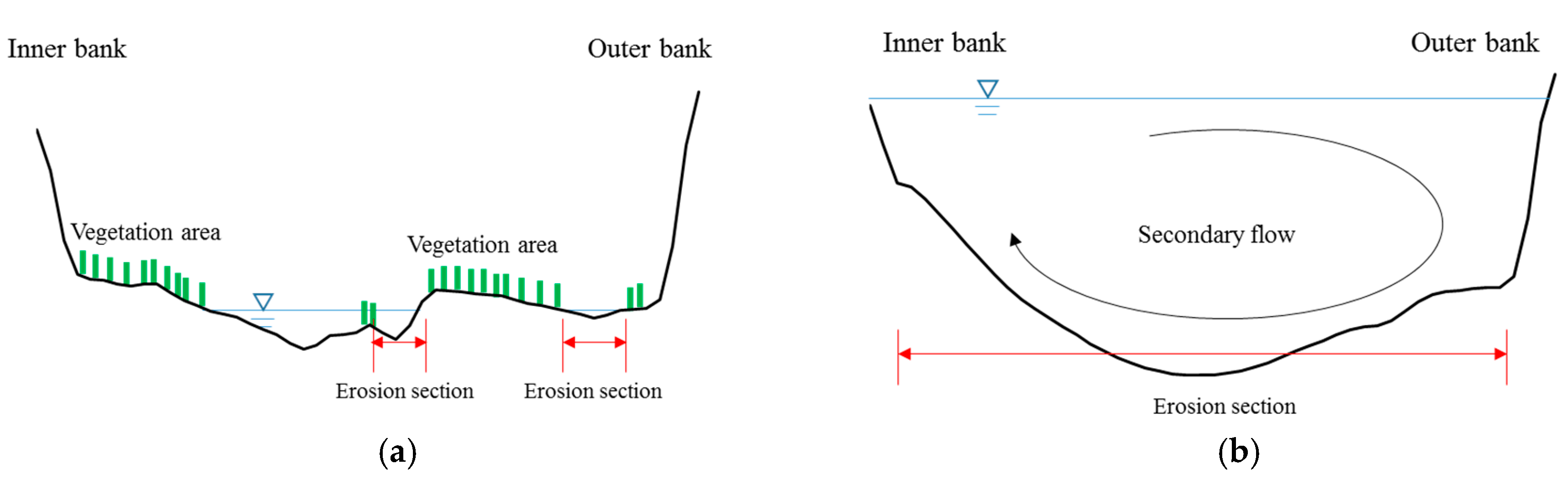
Figure 11.
Final channel patterns depending on growing vegetation and peak discharge. Cases of no growing vegetation: (a,c,e); cases of growing vegetation: (b,d,f); (g) legend of elevation change (m). ”Peak” is peak discharge (m3/s).
Figure 11.
Final channel patterns depending on growing vegetation and peak discharge. Cases of no growing vegetation: (a,c,e); cases of growing vegetation: (b,d,f); (g) legend of elevation change (m). ”Peak” is peak discharge (m3/s).

Figure 12.
Final distribution of permanent vegetation with growing vegetation (red color: permanent vegetation). (a) MF peak discharge: 690 m3/s; (b) AMF peak discharge: 1381 m3/s; (c) EF peak discharge: 2762 m3/s; (d) legend of vegetation growth stage.
Figure 12.
Final distribution of permanent vegetation with growing vegetation (red color: permanent vegetation). (a) MF peak discharge: 690 m3/s; (b) AMF peak discharge: 1381 m3/s; (c) EF peak discharge: 2762 m3/s; (d) legend of vegetation growth stage.
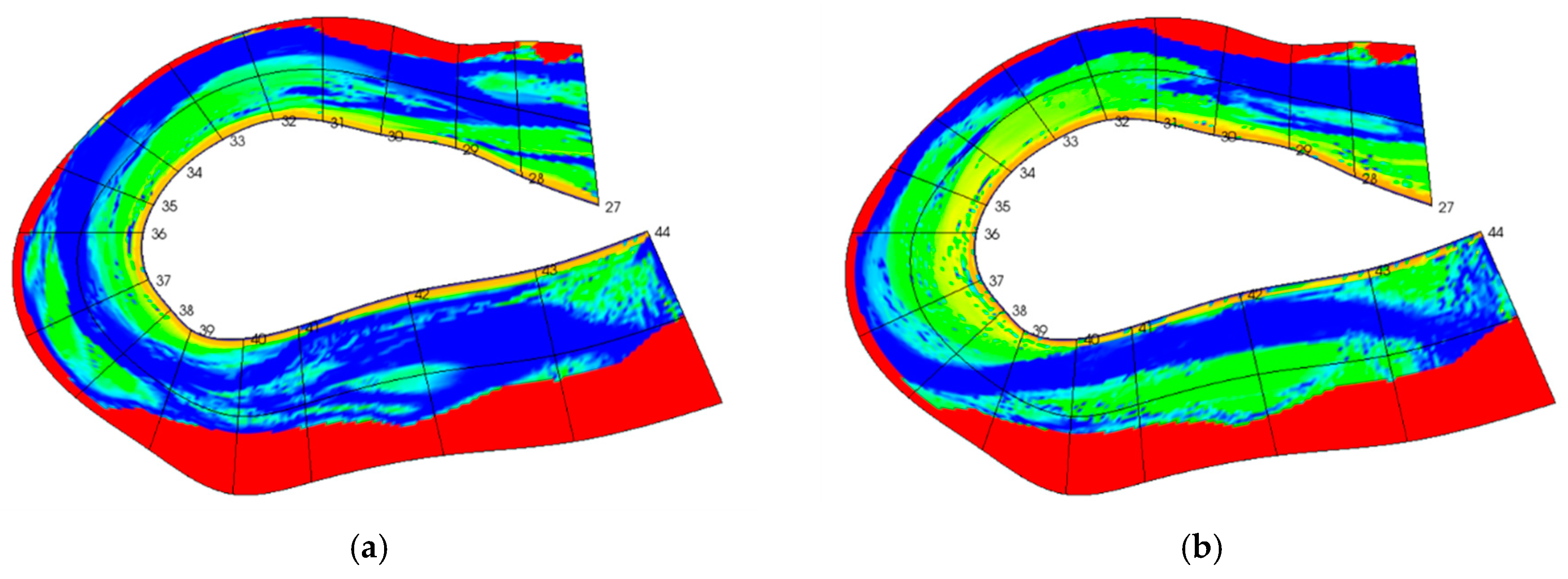
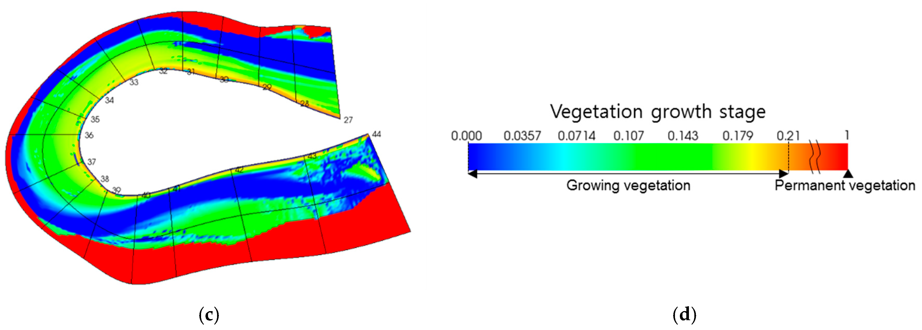
Figure 13.
Temporal change of ABI and BRI. ABI: (a) MF peak discharge: 690 m3/s; (c) AMF peak discharge: 1381 m3/s; (e) EF peak discharge: 2762 m3/s. BRI: (b) MF peak discharge: 690 m3/s; (d) AMF peak discharge: 1381 m3/s; (f) EF peak discharge: 2762 m3/s.
Figure 13.
Temporal change of ABI and BRI. ABI: (a) MF peak discharge: 690 m3/s; (c) AMF peak discharge: 1381 m3/s; (e) EF peak discharge: 2762 m3/s. BRI: (b) MF peak discharge: 690 m3/s; (d) AMF peak discharge: 1381 m3/s; (f) EF peak discharge: 2762 m3/s.

Figure 14.
Cross sectional bed changing depending on vegetation and peak discharge. (a) MF (690 m3/s) peak discharge; (b) AMF (1381 m3/s) peak discharge; (c) EF (2762 m3/s) peak discharge; (d) location of cross section A-A’.
Figure 14.
Cross sectional bed changing depending on vegetation and peak discharge. (a) MF (690 m3/s) peak discharge; (b) AMF (1381 m3/s) peak discharge; (c) EF (2762 m3/s) peak discharge; (d) location of cross section A-A’.


Table 1.
Main computation parameters.
| Parameter | Value | Model |
|---|---|---|
| The von Karman constant (κ) | 0.4 | Zero Equation |
| Mean diameter of bed load ( | 1.49 mm | Sediment transport |
| Manning roughness coefficient () | 0.016 s/m1/3 | Sediment transport |
| Critical Shields number ( | 0.0374 | Sediment transport |
| The number of vegetation in unit area () | 95.34 EA | Vegetation |
| Coefficient of Drag force for vegetation () | 0.7 | Vegetation |
| Maximum growth stage () | 0.21 | Vegetation |
| Critical erosion depth of Vegetation decay (root length) | 0.8 m | Vegetation |
| Angle of repose for bed material ( | 30 | Slope failure |
Table 2.
Simulation conditions depending on discharge.
| No. | Peak Discharge (m3/s) | Total Flood Duration (h) | Growing Vegetation | Permanent Vegetation |
|---|---|---|---|---|
| Run-1 | 690 | 450 | No | Yes |
| Run-2 | 1381 | 450 | No | Yes |
| Run-3 | 2762 | 450 | No | Yes |
| Run-4 | 690 | 450 | Yes | Yes |
| Run-5 | 1381 | 450 | Yes | Yes |
| Run-6 | 2762 | 450 | Yes | Yes |
© 2018 by the authors. Licensee MDPI, Basel, Switzerland. This article is an open access article distributed under the terms and conditions of the Creative Commons Attribution (CC BY) license (http://creativecommons.org/licenses/by/4.0/).
Share and Cite
MDPI and ACS Style
Kang, T.; Kimura, I.; Shimizu, Y. Responses of Bed Morphology to Vegetation Growth and Flood Discharge at a Sharp River Bend. Water 2018, 10, 223. https://doi.org/10.3390/w10020223
AMA Style
Kang T, Kimura I, Shimizu Y. Responses of Bed Morphology to Vegetation Growth and Flood Discharge at a Sharp River Bend. Water. 2018; 10(2):223. https://doi.org/10.3390/w10020223
Chicago/Turabian StyleKang, Taeun, Ichiro Kimura, and Yasuyuki Shimizu. 2018. "Responses of Bed Morphology to Vegetation Growth and Flood Discharge at a Sharp River Bend" Water 10, no. 2: 223. https://doi.org/10.3390/w10020223
Note that from the first issue of 2016, this journal uses article numbers instead of page numbers. See further details here.