Article

A Generalized Semi-Analytical Solution for the Dispersive Henry Problem: Effect of Stratification and Anisotropy on Seawater Intrusion

1
Laboratoire d’Hydrologie et Géochimie de Strasbourg, University of Strasbourg/EOST/ENGEES, CNRS, 1 rue Blessig, 67084 Strasbourg, France
2
Department of Civil Engineering, Sharif University of Technology, P.O. Box 11155-9313 Tehran, Iran
3
National Centre for Groundwater Research & Training and College of Science & Engineering, Flinders University, GPO Box 2100, Adelaide, South Australia 5001, Australia
4
IRD UMR LISAH, F-92761 Montpellier, France
5
LMHE, ENIT, BP 37, 1002 Tunis Le Belvédère, Tunisie
*
Author to whom correspondence should be addressed.
Water 2018, 10(2), 230; https://doi.org/10.3390/w10020230
Submission received: 11 January 2018 / Revised: 15 February 2018 / Accepted: 17 February 2018 / Published: 23 February 2018
(This article belongs to the Special Issue Seawater Intrusion: Simulation and Control)

Abstract

:
The Henry problem (HP) continues to play a useful role in theoretical and practical studies related to seawater intrusion (SWI) into coastal aquifers. The popularity of this problem is attributed to its simplicity and precision to the existence of semi-analytical (SA) solutions. The first SA solution has been developed for a high uniform diffusion coefficient. Several further studies have contributed more realistic solutions with lower diffusion coefficients or velocity-dependent dispersion. All the existing SA solutions are limited to homogenous and isotropic domains. This work attempts to improve the realism of the SA solution of the dispersive HP by extending it to heterogeneous and anisotropic coastal aquifers. The solution is obtained using the Fourier series method. A special hydraulic conductivity–depth model describing stratified heterogeneity is used for mathematical convenience. An efficient technique is developed to solve the flow and transport equations in the spectral space. With this technique, we show that the HP can be solved in the spectral space with the salt concentration as primary unknown. Several examples are generated, and the SA solutions are compared against an in-house finite element code. The results provide high-quality data assessed by quantitative indicators that can be effectively used for code verification in realistic configurations of heterogeneity and anisotropy. The SA solution is used to explain contradictory results stated in the previous works about the effect of anisotropy on the saltwater wedge. It is also used to investigate the combined influence of stratification and anisotropy on relevant metrics characterizing SWI. At a constant gravity number, anisotropy leads to landward migration of the saltwater wedge, more intense saltwater flux, a wider mixing zone and shallower groundwater discharge zone to the sea. The influence of stratified heterogeneity is more pronounced in highly anisotropic aquifers. The stratification rate and anisotropy have complementary effects on all SWI metrics, except for the depth of the discharge zone.

1. Introduction

The Henry problem (HP) [1] is widely used as a surrogate for the understanding of seawater intrusion (SWI) processes in coastal aquifers [2]. It is an abstraction of SWI in a vertical cross-section of a confined coastal aquifer perpendicular to the shoreline. In this aquifer, an inland freshwater flow is in equilibrium with the seawater intruded from the seaside, due to its higher density (Figure 1). The aquifer is assumed to be homogenous and isotropic.
Recently, a variation of the HP has been used to understand SWI in fractured coastal aquifers [4,5]. A reactive HP has been presented to investigate the interplay between dispersion and reactive processes in coastal aquifers [6] and to study the effect of calcite dissolution on SWI [7,8]. HP has been considered in several works investigating the effects of heterogeneity [9,10,11], anisotropy [12,13], mass dispersion [13], salinity dependent permeability [14], seafloor slope [15] and inland boundary conditions [16] on the SWI extent. Three variants of this problem were used in Post et al. [17] to interpret the groundwater ages in coastal aquifers. Javadi et al. [18] developed a multi-objective optimization algorithm and applied it to the HP in order to assess different management methods for controlling SWI. Hardyanto and Merkel [19], Herckenrath et al. [20], Rajabi and Ataie-Ashtiani [21], Rajabi et al. [22,23], Burrows and Doherty [24] and Riva et al. [25] investigated the HP and conducted uncertainty analyses to evaluate the effect of incomplete knowledge of the aquifer parameters on the predictions of SWI models. Sanz and Voss [26] developed an a posteriori parameter covariance matrix analysis of the HP and provided insight about parameter sensitivities that can help in improving the inverse modeling procedure. A parameter sensitivity analysis based on the HP was also reported in Carrera et al. [27], who presented a general analysis of the inverse problem for SWI.
This brief review points out the importance of the HP for theoretical and practical investigations of conceptual and modeling aspects of SWI. Nonetheless, the popularity of this problem stems precisely from the existence of a semi-analytical (SA) solution [1]. The mathematical formulation of the HP is based on the density-driven flow (DDF) model that incorporates a system of a variable density-flow equation, an advection–dispersion equation and a state relation, expressing the mixture density as function of the saltwater concentration. Because of the existence of this SA solution, HP has been accepted as one of the primary benchmarks for the assessment of DDF numerical codes, e.g., [6,28,29,30,31,32,33,34,35,36,37,38,39,40,41,42,43,44,45].
The first SA solution of the HP was developed by Henry [1] using the Fourier series method. This solution underwent a revision by Segol [46], who pointed out some errors in Henry’s solution and proposed appropriate corrections. With this revision, Segol [46] was able to recreate the SA solution numerically. The worthiness of this SA solution for benchmarking DDF codes has been widely discussed in the literature [2,47,48,49,50,51,52,53]. These studies concluded that Segol’s solution is not sufficient to test DDF numerical models since the buoyancy effects are dominated by the influence of boundary forcing exerted by the freshwater inland flow and by the diffusion effects, as the solution was developed for exaggerated diffusion coefficients. Consequently, Simpson and Clement [48] suggested an improved version of the SA solution in which the freshwater recharge was decreased by half. Younes and Fahs [54] and Zidane et al. [55] developed new implementations of the SA method and obtained solutions with reduced diffusion coefficients. Moreover, another limitation of the Henry’s SA solution is its unrepresentativeness of the real-world SWI as only uniform diffusion and no velocity-dependent dispersion is considered. Dispersion processes are important factors that effectively influence the mixing between fresh and salt waters [12,13,56]. A dispersive HP has been suggested by Abarca et al. [13] based on numerical simulations. As claimed by Abarca et al. [13], the major drawback of this problem is that there is no reference solution with which the results can be compared. Recently Fahs et al. [57] addressed this issue and developed a new SA solution for the dispersive HP. While all the existing SA solutions are based on the positions of the main concentration isochlors, Fahs et al. [57] derived, analytically, several metrics, characterizing the SWI as the toe length, thickness of the mixing zone, saltwater flux to the aquifer and depth of the groundwater discharge zone at the sea boundary.
This paper attempts to generalize the SA solution of the dispersive HP to more realistic configurations. Indeed, anisotropy and heterogeneity are primary characteristics of real aquifers that the SA solutions of the HP do not account for. Several former studies indicated that anisotropy can affect the saltwater penetration, the saltwater flux and submarine groundwater discharge [12,13,58]. Heterogeneity has been also found to play an important role in SWI processes [9,10,59,60,61]. Thus, the aim of this paper is to extend the SA solution of the dispersive HP, developed by Fahs et al. [57], to anisotropic and heterogeneous coastal aquifers.
The developed SA solution is based on the Fourier series method, applied to the stream function form of the governing equations. This method combines the exactness of the analytical methods with an important extent of generality in describing the geometry and boundary conditions of the numerical methods [62]. It proceeds by expending the unknowns (stream function and salt concentration) into infinite Fourier series and applying a Galerkin treatment using the Fourier modes as trial functions. We derived the stream function formulation for flow in heterogeneous and anisotropic domain. Heterogeneity introduces terms involving the space derivative of the permeability that require specific permeability–depth relationships to be addressed analytically. This was achieved by considering a stratified domain characterized via the Gardner exponential permeability function [63], which is widely used in layered aquifers, e.g., [64,65,66,67,68,69,70]. Solving the flow and transport equations in the spectral space is a challenging task, especially when large numbers of Fourier modes should be used to obtain oscillation-free solutions. Heterogeneity compounds these challenges as it involves high local gravity numbers that require a large number of Fourier modes to be represented adequately [71]. A new technique is developed here for solving the spectral flow and transport equations with a reduced number of unknowns. With this technique, we show that the HP can be solved in the spectral space with only the concentration as the primary unknown.
Various illustrative test cases are generated, and the SA solutions are compared against an in-house finite element code. The SWI metrics are evaluated analytically based on the Fourier series. These metrics represent quantitative indicators more suitable for code validation and benchmarking than the isochlors’ positions. They are also used to investigate the effects of anisotropy and stratified heterogeneity on SWI. Indeed, few studies have reported the effect of anisotropy on the isochlors’ positions [12,13,58]. The contradictory results of these studies call for further investigations [12]. In addition, the effect of heterogeneity on SWI has been considered experimentally and numerically in [10,61,72,73,74]. To the best of our knowledge, coupled effects of anisotropy and stratified heterogeneity have never been investigated. Here, we take advantage of the developed SA solution to address this gap. Moreover, while previous numerical or experimental studies investigated, visually, the uncoupled effects of anisotropy and stratification on the isochlors, this work aims to analytically provide a deeper understanding of their coupled effects on several relevant metrics characterizing SWI.

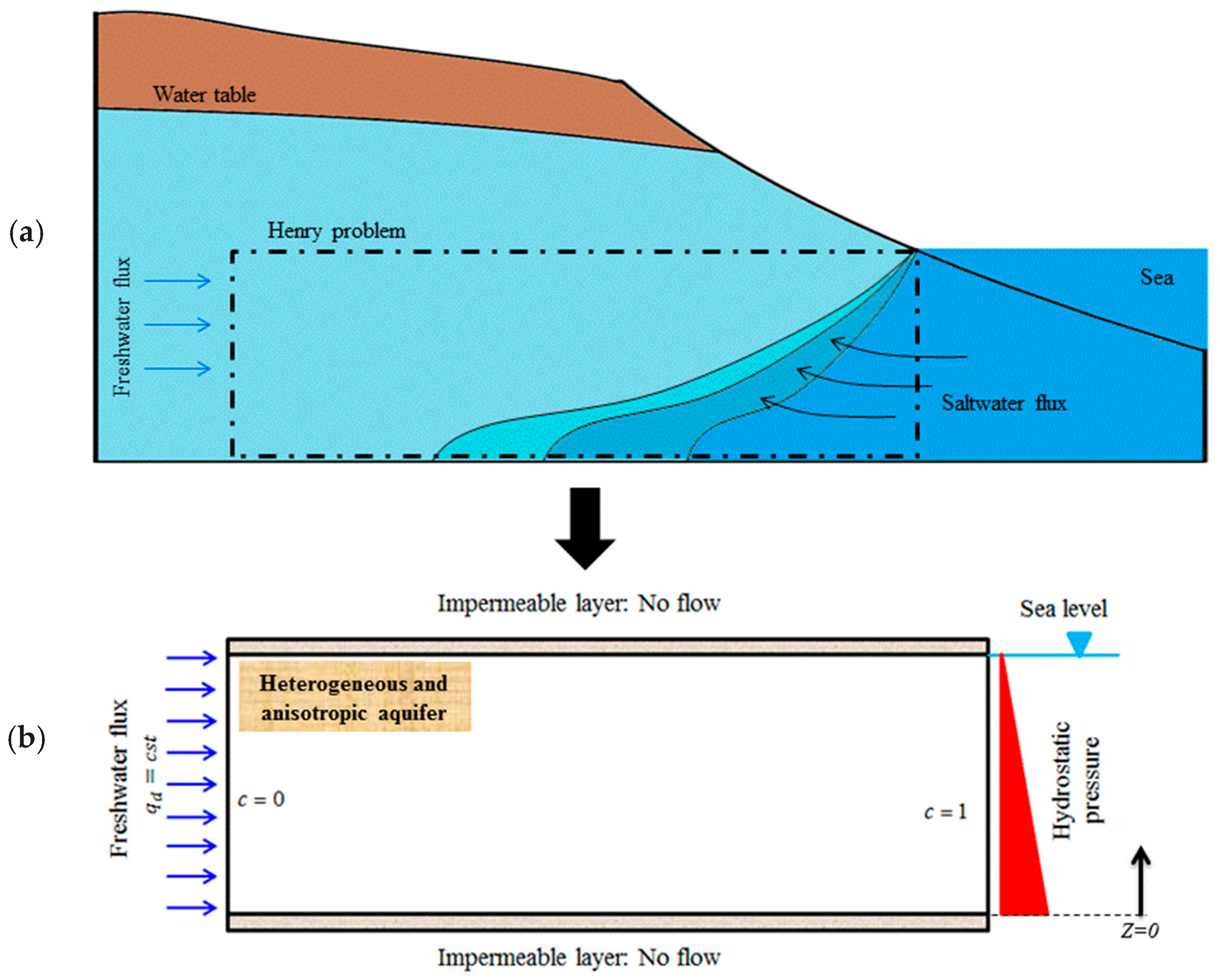
2. The Mathematical Model and Boundary Conditions

The DDF mathematical model for SWI is based upon the coupled variable-density flow and mass transport equation. Under the Oberbeck–Boussinesq approximation [75] and steady-state conditions, the flow system is given by the following continuity equation and Darcy’s law [76]:
q = 0 ,
q = K ( h + ρ ρ 0 ρ 0 z ) ,
where q is the Darcy’s velocity [ L T 1 ] ; ρ 0 is the freshwater density [ M L 3 ] ; K is the freshwater hydraulic conductivity tensor [ L T 1 ] (diagonal with components K x and K z ); h is the equivalent freshwater head [ L ] ; ρ is the density of mixture fluid [ M L 3 ] and z is the elevation [ L ] .
The salt transport processes can be described by the advection–dispersion equation:
ε c t + q c ( ε D m I + D ) c = 0
where c is the dimensionless solute concentration [ ] ; D m is the molecular diffusion coefficient [ L 2 T 1 ] ; ε is the porosity [ ] , I is the identity matrix and D is the dispersion tensor defined by:
D = ( α L α T ) q × q | q | + α T | q | I
where α L and α T are the longitudinal and transverse dispersion coefficients, respectively [ L ] .
The flow and transport equations are coupled via the linear mixture density equation:
ρ = ρ 0 + Δ ρ . c ,
where Δ ρ = ρ 1 ρ 0 is the density difference between seawater ( ρ 1 ) and freshwater ( ρ 0 ).
The geometry of the aquifer is simplified to a rectangle of length ( ) and depth ( d ) . The freshwater recharge flux per unit of width imposed on the inland side is noted as q d [ L 2 T 1 ] . At the seaside, the seawater’s equivalent freshwater head is specified and constant salt concentration (c = 1) is imposed.

3. The Semi-Analytical Solution
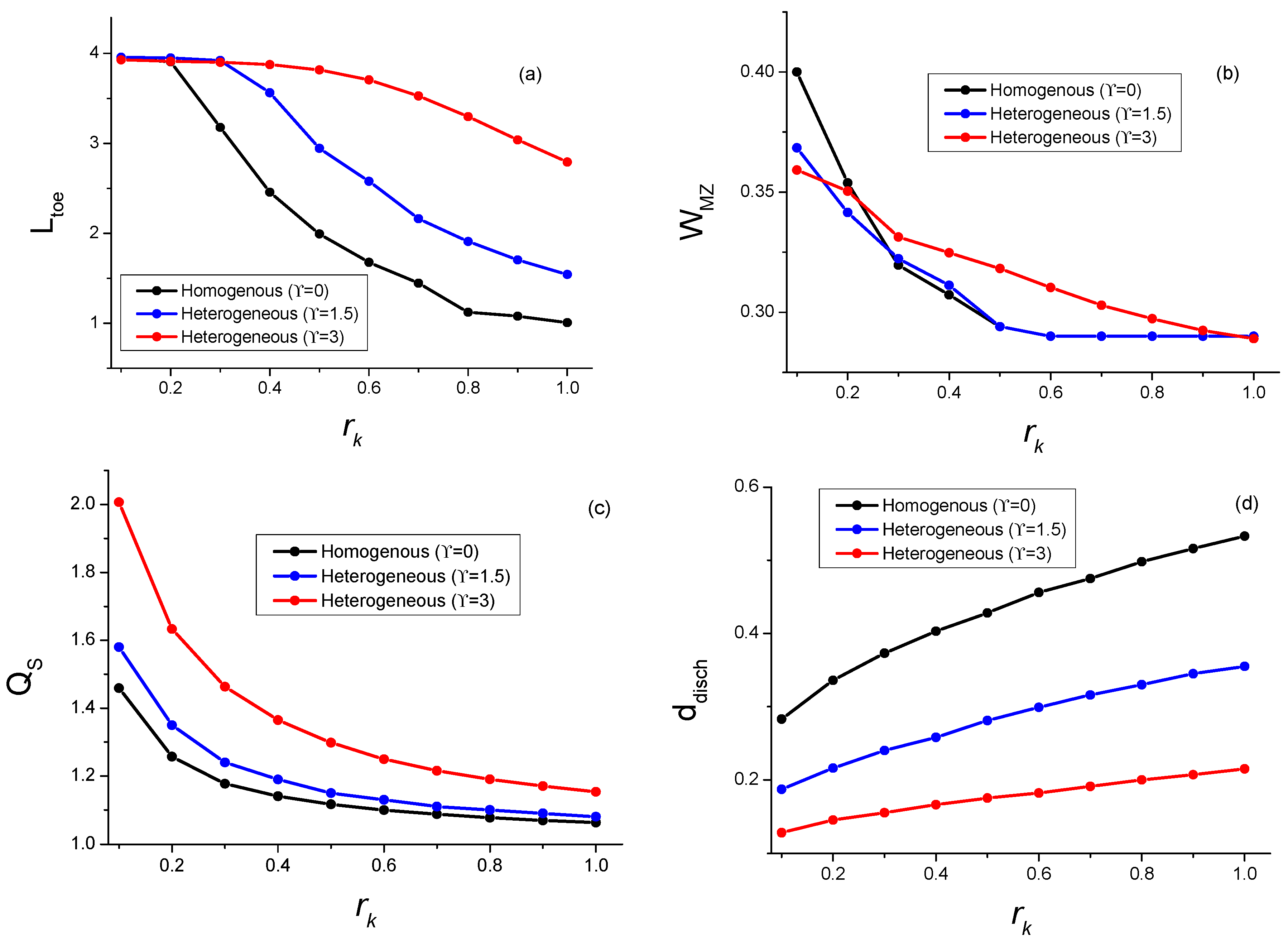
In isotropic domains, the freshwater head (h) can be eliminated from the flow equation by applying the curl operator to Darcy’s law. For the anisotropic domain, an equivalent procedure is to differentiate the x-component (respectively, z-component) of Darcy’s law with respect to z (respectively, x) and divide it by K x (respectively, K z ), while accounting for spatial hydraulic conductivity variation, as the domain is heterogeneous. Subtracting the resulting equations, one from the other, gives:
r K q x z q z x = K z ρ 0 ρ x + r K q x 1 K x K x z q z 1 K z K z x ,
where q x and q z are the velocity components and r K = K z / K x is the hydraulic conductivity anisotropy ratio, as defined in Abarca et al. [13].
The stream function ( ψ ), defined by q x = ψ / z and q z = ψ / x , can satisfy the continuity equation. Using Equation (5) and the stream function, Equation (6) is written as:
r K 2 ψ z 2 + 2 ψ x 2 r K ψ z 1 K x K x z ψ x 1 K z K z x K z Δ ρ ρ 0 c x = 0 .
As in the standard HP, the following changes in variables are considered to obtain periodic boundary conditions (essential for the Fourier series method) and to derive the non-dimensional form of the flow equation (the complete mathematical development can be found in [46,55,57]):
X = x d ,   Z = z d ,   Ψ = ψ q d   Z ,   C = c X ξ ,
where ξ = / d is the aspect ratio.
r K 2 Ψ Z 2 + 2 Ψ X 2 r K 1 K x K x Z ( Ψ Z + 1 ) + 1 K z K z X Ψ X N G ( C X + 1 ξ ) = 0 ,
where N G = K z d Δ ρ / ρ 0 q d is the local gravity number which compares the buoyancy flux to the inland freshwater flux.
Due to heterogeneity, the stream function formulation of the flow equation incorporates the spatial derivatives of the hydraulic conductivity. Consequently, the SA solution cannot be obtained under discontinuous depth–hydraulic conductivity relationship. To overcome this limitation, we considered heterogeneities corresponding to vertical stratification. This picture is widespread and agrees with several coastal sedimentary aquifers [61,77]. We assume that heterogeneity is perfectly layering with an exponential trend of hydraulic conductivity with depth. The exponential trend of hydraulic conductivity has been suggested as a simplified model to describe stratified heterogeneity by Gardner [63]. It appears to have considerable generality and field evidence [64,65,66,67,68,69,70]. In anisotropic aquifers, the exponential depth–hydraulic conductivity model was suggested by Zlotnik et al. [68]:
K x ( Z ) = K x , 0 e ϒ Z ;   K z ( Z ) = K z , 0 e ϒ Z ,
where K x , 0 and K z , 0 are the local horizontal and vertical hydraulic conductivities at the aquifer bottom surface, respectively. ϒ is the rate of hydraulic conductivity change with depth.
Usually, the hydraulic conductivity is decreasing with depth. Thus, ϒ is mostly positive. In certain cases, hydraulic conductivity can increase with depth ( ϒ negative) due to hydro-fracturing. The developed SA method can be applied to both negative and positive values of ϒ , but results are presented only for the common case of decreasing hydraulic conductivity with depth. The considered model (Equation (10)) assumes constant local (or small) scale anisotropy, as the anisotropy ratio is the same for all layers ( r K = K z / K x = K z , 0 / K x , 0 ). Based on the adopted depth–hydraulic conductivity model, Equation (9) becomes:
r K 2 Ψ Z 2 + 2 Ψ X 2 ϒ r K ( Ψ Z + 1 ) N G 0 e ϒ Z ( C X + 1 ξ ) = 0 ,
where N G 0 ( = K z , 0 d Δ ρ / ρ 0 q d ) is the local gravity number at the aquifer bottom surface.
The boundary conditions for Equation (11) are given by (see Fahs et al. [57]):
Ψ X ( 0 , Z ) = Ψ X ( ξ , Z ) = C ( 0 , Z ) = C ( ξ , Z ) = 0 , Ψ ( X , 0 ) = Ψ ( X , 1 ) = C Z ( X , 0 ) = C Z ( X , 1 ) = 0 ,
The unknowns are expanded into infinite Fourier series that satisfy the boundary conditions:
Ψ = m = 1 N m n = 0 N n A m , n sin ( m π Z ) cos ( n π X / ξ ) ,
C = r = 0 N r s = 1 N s B r , s cos ( r π Z ) sin ( s π X / ξ ) ,
where A m , n (respectively, B r , s ) are the Fourier series coefficients for the stream function (respectively, concentration). N m and N n are the truncation orders for the stream function in the X and Z directions, respectively. N r and N s are the ones for the salt concentration.
The Fourier series expansions are appropriately substituted into Equation (11). Then, a Galerkin treatment is applied, with the Fourier modes as trial functions. This leads to the following system of equations:
R g , h F = ϖ h 1 π 2 ξ A g , h ( r k g 2 + h 2 ξ 2 ) + ϖ h 1 r K ϒ ξ m = 1 N m m A m , h Π g , m + π 2 N G 0 h r = 0 n r B ˜ r , h Γ g , r + 2 π N G 0 δ h , 0 Γ g , 0 + 2 r K ϒ ξ π Π g , 0 δ h , 0 = 0         ( g = 1 .. N m ,    h = 0 .. N n ) ,
where R F is the residual vector of the flow equation and δ i , j is the Kronecker symbol.
The above procedure is similarly applied to the transport equation. This gives:
b m ( 2 C X 2 + 2 C Z 2 ) Ψ Z C X + Ψ X C Z 1 ξ Ψ Z C X 1 ξ + Δ 1 , 1 2 C X 2 + 2 Δ 1 , 2 2 C X Z + Δ 2 , 2 2 C Z 2 + ( C X + 1 ξ ) ( Δ 1 , 1 X + Δ 1 , 2 Z ) + C Z ( Δ 1 , 2 X + Δ 2 , 2 Z ) = 0 ,
where b m = ε D m / q d and Δ i , j = D i , j / q d .
The Fourier series method applied to Equation (16) gives the following system of equations (see Fahs et al. [57]):
R g , h T = ϖ g 2 b m π 2 B g , h ( h 2 ξ 2 + g 2 ) ξ π 4 m = 1 N m n = 0 N n r = 0 N r s = 1 N s B r , s A m , n ( s . m . η g , m , r θ h , n , s r . n . κ g , m , r λ h , n , s ) g n = 0 N n A ˜ g , n Λ h , n ϖ g 2 s = 1 N s s B g , s Λ h , s 2 π Λ h , 0 δ g , 0 4 i = 1 N p W p i F D i s p ( X p i , Z p i ) cos ( g π Z p i ) sin ( h π X p i ξ ) = 0      ( g = 0 .. N r ; h = 1 .. N s ) ,
where R T is the residual vector corresponding to the transport equation. The coefficients and matrices of Equations (15) and (17) are defined in Appendix A. N p is the number of integration points used to evaluate the dispersion terms. W p , X p and Z p are the integration weight and the coordinates of the integration points, respectively.
We should mention that, as in Fahs et al. [57], the Fourier series are used to evaluate analytically the four dimensionless metrics characterizing the SWI:
  • The length of the toe ( L t o e ): The dimensionless distance between the seaside boundary and the point where the 50% isochlor intersects the aquifer bottom.
  • The average vertical width of the mixing zone ( W M Z ): Defined as the average of the vertical dimensionless distances between the 10% and 90% isochlors. The mixing zone is defined by the interval 0.3 × L t o e to 0.7 × L t o e .
  • The total dimensionless salt flux ( Q s ): Represents the advective, diffusive and dispersive salt flux that enters the domain from the seaside boundary, normalized by the freshwater inland flux.
  • The depth of the zone of groundwater discharge to the sea ( d d i s c h ): Equal to the distance from the aquifer top surface to the point separating the discharge zone and seawater inland flow zone at the sea boundary.

4. The New Technique for Solving the System of Equations in the Spectral Space

Solving the coupled system of flow and salt transport of the HP in the spectral space (Equations (15) and (17)) is not an easy task, particularly for cases involving a large numbers of Fourier modes. Henry [1], Segol [46] and Simpson and Clement [48] employed the Picard method and solved the system by a sequential procedure between Equations (15) and(17). This approach is computationally efficient because it splits the system into two smaller systems. However, it cannot converge for high nonlinear cases. This is why the first solutions of the HP were limited to high diffusion coefficients with relatively small number of Fourier modes. Zidane et al. [55] solved the system simultaneously using the Newton method with a numerical approximation of the Jacobian matrix. This method provides better convergence properties, but it is limited in computational efficiency, as both flow and transport equations are solved simultaneously in one large system. Younes and Fahs [54] tried to circumvent this drawback by using the Powell algorithm (a variation of Newton’s method) with the analytical Jacobian matrix. In the present work, we develop a new technique that preserves the same convergence property as the one developed by Younes and Fahs [54], but without scarifying computational efficiency of the sequential resolution (i.e., solving small systems). We show that the flow (stream function) can be analytically calculated in terms of the salt concentration, and the spectral transport equation can be solved via Newton’s method, with only the Fourier series coefficients of the salt concentration as primary unknowns.
The proof is firstly developed for homogenous aquifer. In this case, the second and fifth terms of Equation (15) drop out. This allows explicit calculation of the Fourier series coefficients of the stream function in terms of the ones for salt concentration. This gives:
A i , j = 1 π ξ N G 0 ϖ j 1 π j r = 0 N r B ˜ r , j Γ i , r + 2 δ j , 0 Γ i , 0 r k i 2 + j 2 / ξ 2 .
Equation (18) is then substituted into Equation (17). This eliminates the coefficient A g , h :
R g , h T = ϖ g 2 b m π 2 B g , h ( h 2 ξ 2 + g 2 ) ξ + N G 0 4 ξ m = 1 N m n = 0 N n r = 0 N r s = 1 N s B r , s 1 ϖ n 1 π n r = 0 N r B ˜ r , n Γ m , r + 2 δ n , 0 Γ m , 0 r k m 2 + n 2 / ξ 2 ( s . m . η g , m , r θ h , n , s r . n . κ g , m , r λ h , n , s ) + g N G 0 π ξ n = 0 N n 1 ϖ n 1 π n r = 0 N r B ˜ r , n Γ g , r + 2 δ n , 0 Γ g , 0 r k g 2 + n 2 / ξ 2 Λ h , n ϖ g 2 s = 1 N s s B g , s Λ h , s 2 π Λ h , 0 δ g , 0 4 i = 1 N p W p i F D i s p ( X p i , Z p i ) cos ( g π Z p i ) sin ( h π X p i ξ ) = 0 .
In the case of a heterogeneous domain, expression of A i , j in Equation (18) can be obtained explicitly by considering the matrix form of Equation (18):
[ M ] . A = [ N ] . B + V ,
where M is the matrix coefficients of A g , h (first two terms in Equation (15)), N is the matrix coefficients of B g , h (third term in Equation (15)), A and B are two vectors representing, respectively, the Fourier series coefficients, A g , h and B g , h , and V is a constant vector (last two terms in Equation(15)).
Equation (19) represents a closed system of ( N r + 1 ) × N s equations with the coefficients B g , h as unknowns. This system can be solved alone without any coupling with the flow equation. In this work, we solved it using the nonlinear solver of the IMSL library. The Jacobian matrix is provided analytically and the term with four nested summations is simplified to three summations, as in Fahs et al. [57]. Similarly, the three resolving steps (i.e., residual vector, Jacobian matrix and linear system) are implemented in parallel on shared memory architecture.

5. Verification of the Fourier Series Solution: Stability and Comparison against Numerical Solution

A FORTRAN code has been developed to solve the final system of nonlinear equations resulting from the Fourier series method. To examine the correctness of this code, we compared it against a full numerical solution obtained using an advanced in-house model [32]. The numerical model is based on the combination of the method of lines for higher order time integration and advanced methods for spatial discretization. The mixed hybrid finite element method, which is appropriate for anisotropic and heterogeneous domains, is used to solve the flow equation. The transport equation is discretized based on the discontinuous Galerkin finite element method that can accurately handle sharp solutions with relatively coarse meshes [32]. The numerical simulations are performed with a fine mesh involving 10,000 triangular elements, obtained by subdividing 2500 squares into four equal triangles. This regular mesh is used to avoid numerical artifacts related to irregular meshes. All the simulations are developed under a transient regime for a long duration to reach the steady-state solution.
Besides validation, this section aims also to investigate the effects of heterogeneity and anisotropy on the stability of the Fourier series solution. As mentioned previously, the anisotropic layered aquifers considered in our study are described by the exponential depth–hydraulic conductivity model. Four test cases, based on the standard pure diffusive [1] and dispersive HP [13], are generated. The results are compared in terms of isochlors’ positions and SWI metrics ( L t o e , W M Z , Q s and d d i s c h ). For an adequate comparison, we assume the same effective large-scale gravity number for all the cases. The large-scale gravity number is calculated based on the average hydraulic conductivity ( K z ¯ ):
N G ¯ = K z ¯ d Δ ρ ρ 0 q d .
The average hydraulic conductivity (in the vertical direction) for layered aquifers with depth-dependent hydraulic conductivity is given by [68]:
K z ¯ = 1 0 1 d Z K z ( Z ) = K z , 0 ϒ 1 e ϒ .
Thus, the large-scale gravity number is calculated as follows:
N G ¯ = ϒ 1 e ϒ N G 0 .
For all cases, the domain aspect ratio ( ξ ) is increased to 4. This is to ensure perfect horizontal streamlines at the land boundary, essential to satisfy the freshwater recharge boundary conditions with the Fourier series solution [55].

5.1. The Pure Diffusive Henry Problem

Two pure diffusive cases are considered using the same parameters as in the standard HP [1]. The first case deals with a homogenous domain ( ϒ = 0 ) while, in the second one, the aquifer is assumed to be stratified ( ϒ = 1.5 ). Anisotropy is acknowledged with r k = 0.66 , as in Abarca et al. [13]. The variations of K x and K z with depth are given in Figure 2. The non-dimensional parameters used for these cases are given in Table 1. The corresponding physical parameters used in the numerical code are summarized in Table 2.
For the homogenous case, the SA solution for the anisotropic domain is sought using 1868 Fourier modes ( N m = 8 , N n = 40 , N r = 10 and N s = 140 ), similar to the isotropic domain in Fahs et al. [57]. This indicates that anisotropy does not affect the stability of the Fourier series solution. For the heterogeneous case, the same number of Fourier modes leads to an unstable SA solution with some unphysical oscillations at the aquifer top (Figure 3). In fact, in this upper zone, the local permeability is five times more important than at the aquifer bottom. This high permeability leads to stronger buoyancy effects than in the homogenous case. The buoyancy forces act on a smaller space scale than convection–dispersion processes and require, consequently, a higher number of Fourier modes to be accurately simulated [71]. An oscillation-free solution has been obtained with 2968 coefficients ( N m = 8 , N n = 40 , N r = 10 and N s = 240 ). Several runs confirm that heterogeneity affects only the truncation order of the concentration Fourier series in the x-direction. The SA and numerical isochlors are plotted in Figure 4. The corresponding SWI metrics are given in Table 3. Results show an excellent agreement between the SA and numerical solutions. This gives more confidence in the correctness of both numerical and SA codes. The agreement between the numerical and SA values of Q s is less than for the other metrics. This can be explained by the fact that Q s involves the x-derivative of the concentration that is very sensitive to the Fourier modes (in the SA solution) and the mesh size (in the numerical solution).

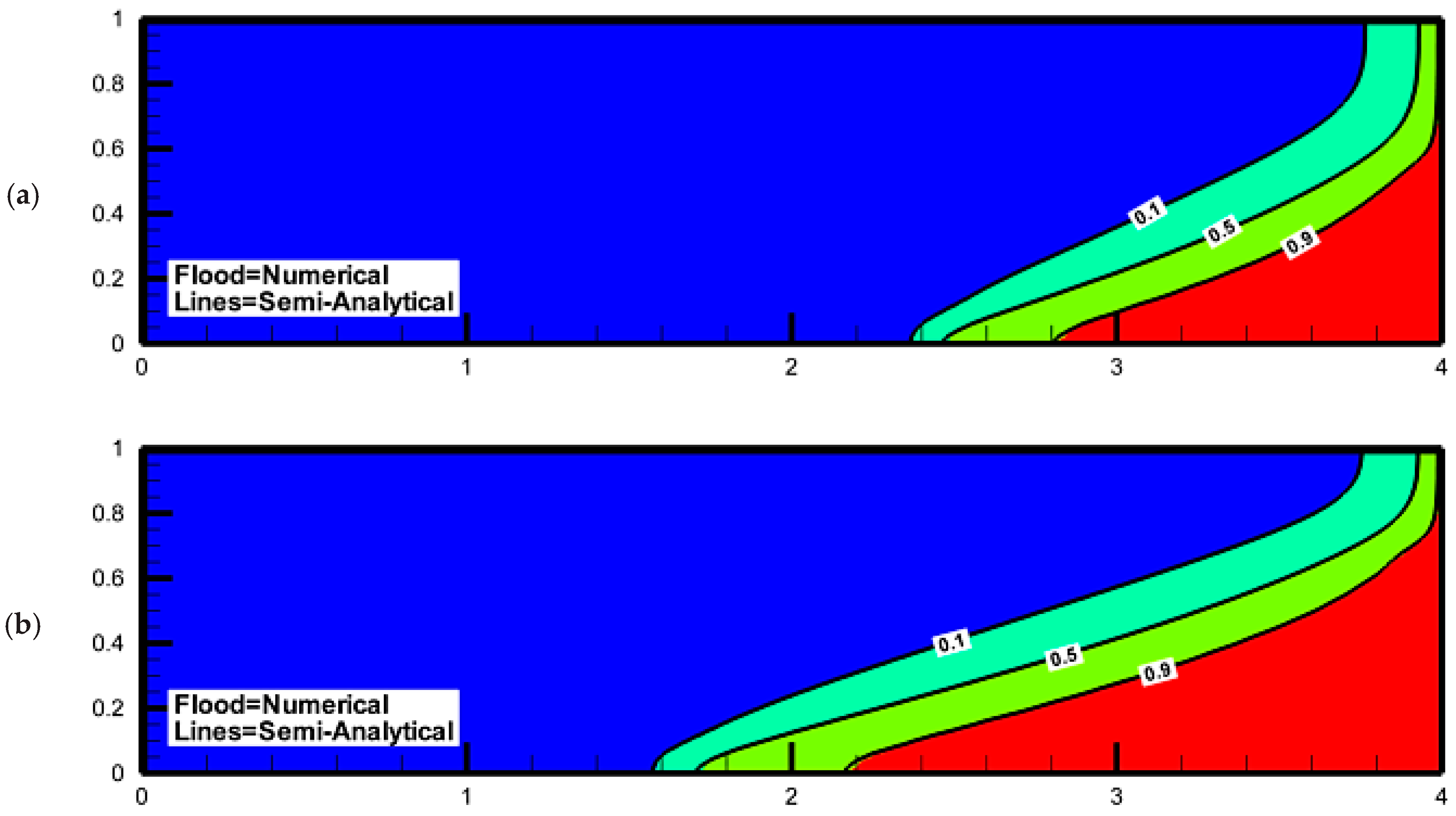
5.2. The Dispersive Henry Problem

For the dispersive HP, all parameters are set as in Abarca et al. [13], except for the molecular diffusion coefficient ( b m ) which is, for convenience, assumed to be very small (5 × 10⁻⁴) [57]. The anisotropy ratio ( r k ) and the rate of stratification ( ϒ ) are kept the same as for the pure diffusive cases. Non-dimensional and corresponding physical parameters are given in Table 1 and Table 2. For homogenous and heterogeneous cases, oscillation-free solutions have been obtained using 4725 ( N m = 15 , N n = 90 , N r = 20 and N s = 160 ) and 6,405 ( N m = 15 , N n = 90 , N r = 20 and N s = 240 ) Fourier modes, respectively. This confirms that only the concentration Fourier modes in the x-direction are mainly affected by heterogeneity. The SA and numerical isochlors are depicted in Figure 5. SWI metrics are given in Table 3. As for the homogenous case, Figure 5 and Table 3 highlight the excellent agreement between the analytical and numerical solutions. The same remark, as in the homogenous case, can be made regarding the agreement between SA and numerical values of Q s . Table 3 provides quantitative indicators that can be useful for benchmarking DDF codes in realistic configurations of anisotropy and heterogeneity. First an observation from the comparison between the Figure 4 and Figure 5 indicates that the effect of heterogeneity on SWI is more important in the dispersive case. Figure 5 shows that the solution of the dispersive HP is sharper and more realistic than for the diffusive case. This sharpness explains why the dispersive test case requires more Fourier modes than the diffusive one.
It should be noted that, with the new technique developed here for solving the HP in the spectral space, the solution can be obtained with a reduced number of unknowns. For instance, in the pure diffusive homogenous case, the final system to be solved involves about 1400 coefficients, instead of 1868. For more complex cases, such as the heterogeneous dispersive case, the final system is solved with 4800 unknowns, instead of 6405.

6. Effects of Anisotropy and Heterogeneity on SWI

6.1. Effect of Anisotropy on SWI in a Homogenous Aquifer

The effect of anisotropy on SWI has been often investigated using the sharp interface model [77], which assumes that freshwater and saltwater are immiscible [78,79,80,81]. Abarca et al. [13] were the first to investigate the influence of anisotropy on the saltwater wedge using the DDF model. They demonstrated that a decrease in the anisotropy ratio ( r K = K z / K x ) pushes the saltwater wedge landward. Michael et al. [58] studied numerically (based on the DDF model) the effect of anisotropy on the position of the salinity transition zone. They showed that for a lower value of the vertical hydraulic conductivity relative to a constant horizontal conductivity (i.e., lower value of r K = K z / K x ), the salinity transition zone moves seaward and can occur farther offshore. Qu et al. [12] investigated the effect of anisotropy on salinity distribution in an unconfined aquifer. Their results show that the toe recedes when the ratio of horizontal to vertical hydraulic conductivity increases (i.e., r K = K z / K x decreases). The results obtained by Qu et al. [12] and Michael et al. [58] are coherent but they are in contradiction with Abarca et al. [13]. This contradiction was reported in Qu et al. [12]. The authors tried to explain it by simulating their SWI problem with vertical sea–land boundaries (similar to [13]) and showed that the freshwater–seawater interface also moves seaward as r K decreases. In this section, we aim to take advantage of the developed SA solution to provide a better understanding of the effect of anisotropy on SWI. Our goal is to (i) explain the contradictory results of the previously mentioned studies and (ii) investigate the effect of anisotropy, not only on isochlors’ positions, but also on several relevant metrics characterizing the SWI.
Thus, we considered again the dispersive homogenous configuration described above in Table 2. We derived the SA solution for different cases dealing with an increasing anisotropy ratio from 0.1 to 1. Specific Fourier modes are used to obtain a stable solution for each case. Figure 6 represents the salinity distribution for three selected values of r K (0.2, 0.5 and 0.8). This figure shows that the saltwater wedge moves landward with a decrease in r K . It confirms, analytically, the results of Abarca et al. [13]. The contradiction with the results of Michael et al. [58] and Qu et al. [12] can be explained based on the non-dimensional analysis presented in Section 2. In fact, Michael et al. [58] and Qu et al. [12] changed the anisotropy ratio by changing the vertical hydraulic conductivity ( K z ) while keeping the horizontal conductivity ( K x ) constant. This means that the isochlors’ positions are investigated at different gravity numbers as the latter is based on the vertical hydraulic conductivity ( N G = K z d Δ ρ / ρ 0 q d ). In this work, as well as in Abarca et al. [13], K z is kept constant and r K is varied based on K x . This means that the isochlors’ positions are compared at a constant N G . In Michael et al. [58] and Qu et al. [12] the decrease in K z will decrease both r K and N G . The decrease in N G can be alternatively seen as an increase in q d which expresses the intensification of the advection effects related to the inland freshwater recharge against the buoyancy effects (responsible for SWI). This explains why the seawater–freshwater interface is pushed back seaward when r K is decreased in Michael et al. [58] and Qu et al. [12]. In Abarca et al. [13], as well as in this work, increasing K x is equivalent to decreasing r K at a constant gravity number. At a fixed balance between the advection and buoyancy effects, the increase in horizontal permeability ( K x ) intensifies the horizontal flow of seawater. Consequently, the saltwater wedge moves landward. To verify this conclusion, we re-evaluated the SA solution of the homogenous dispersive case by decreasing vertical hydraulic conductivity. The results are illustrated in Figure 7, which confirms that, when the decrease in r K is obtained by decreasing the vertical hydraulic conductivity, the saltwater wedge moves seaward.
Figure 8 presents the variations of L t o e , W M Z , Q s and d d i s c h with respect to r K . Results for the homogenous case are plotted in black solid lines. Figure 8a shows that L t o e decreases with the increase of r K , which is coherent with the results in Figure 6. Figure 8b indicates that the average width of the mixing zone decreases also with r K . This means that anisotropy reduces the mixing between freshwater and intruded saltwater.
Figure 8c shows that the saltwater flux to the aquifer is also controlled by the anisotropy. It decreases with the increase of r K . Qu et al. [12] studied the influence of anisotropy on the submarine groundwater discharge flow. They demonstrated that the freshwater discharge is independent of anisotropy, while the seawater recirculation rate decreases as K x / K z increases. This is in contradiction with our results which is understandable as in Qu et al. [12] r K is changed based on K z which means that the gravity number is not constant. To explain the variation of Q s against r K , let us interpret the increase of r K at constant gravity number as a decrease of the horizontal hydraulic conductivity ( K x ). The horizontal flow near the sea–aquifer interface, which mainly depends on K x , is attenuated and consequently reduces the advective saltwater flux. A closer look at the saltwater flux confirms that the advective saltwater flux is mostly influenced by r K . It decreases when r K is increased. From Figure 8d we can observe that the depth of the zone of groundwater discharge to the sea increases with r K . This is also related to the drop of horizontal velocity near the sea boundary which pushes the inflection point of the velocity downward.

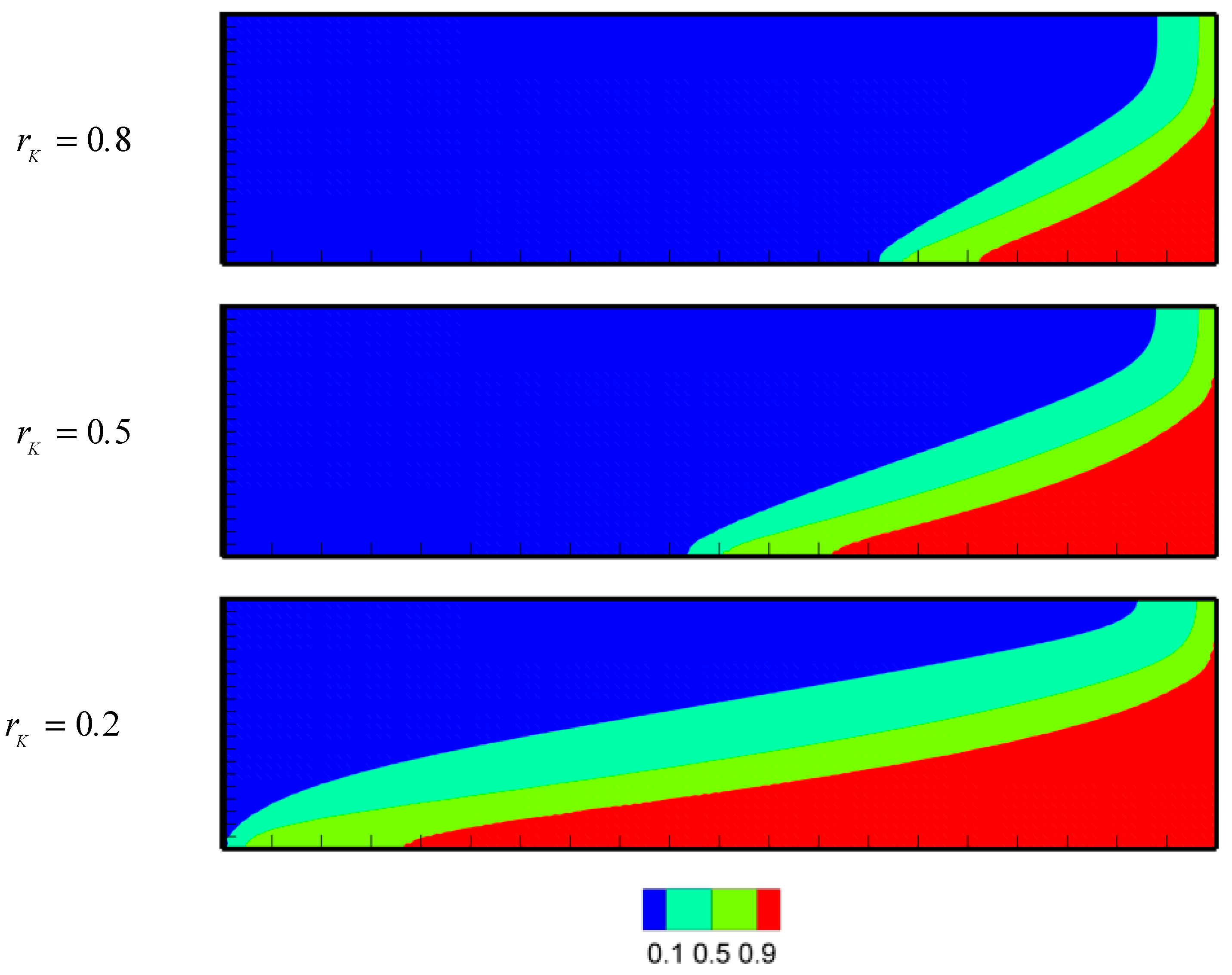
6.2. Coupled Effect of Anisotropy and Stratified Heterogeneity on SWI

Significant research has been devoted to the evaluation of the influence of heterogeneity on SWI [9,10,60,72]. Particular attention has been paid to the stratified heterogeneity using the sharp interface model [77,82,83,84]. The influence of stratification on SWI has been also investigated experimentally and numerically (using the DDF model) [61,77,85]. All these studies focused on the effect of stratified heterogeneity on the isochlors’ positions. Very limited works have investigated the influence of stratification on the thickness of the mixing zone and saltwater flux to the aquifer [61]. On the other hand, combined effects of anisotropy and heterogeneity on solute transport mechanisms have been demonstrated in Qin et al. [86] and Woumeni and Vauclin [87]. Few studies have considered the combined effects of these on SWI [72]. To the best of our knowledge, the combined effects of stratification and anisotropy on SWI have been never discussed in previous studies. Here, we used the SA solution to address these gaps. To do so, we evaluated the SA solutions for two cases dealing with increased rates of heterogeneity ( ϒ = 1.5 and 3 ) and a constant large-scale gravity number ( N G ¯ = 3.11 ). We should mention that exponent ϒ is assumed to be positive. This corresponds to a decreasing hydraulic conductivity with depth which is naturally prevalent in coastal aquifers.
For each case of heterogeneity, the SA is evaluated for increasing anisotropy ratio from 0.1 to 1. The main isochlors (10%, 50% and 90%) for three selected values of r K (0.2, 0.5 and 0.8) in the case of homogenous and heterogeneous (both ϒ = 1.5 and 3 ) aquifers are depicted in Figure 9. This figure shows that the anisotropy and rate of stratification ( ϒ ) have complementary effects on the position of the isochlors. As for the homogenous case, increasing anisotropy pushes the saltwater wedge landward. At a constant large-scale gravity number, the increase in the heterogeneity rate leads also to a landward migration of the transition zone. This is not in agreement with the results of Lu et al. [61] (see Figure 8 in their paper). This disagreement is related to the gravity number. The results presented by Lu et al. [61] were obtained using two different large-scale gravity numbers. In Lu et al. [61], the average vertical hydraulic conductivities were 10 4 and 2.7 × 10 5 m/s for the homogenous and increasing stratified permeability, respectively. Thus, the large-scale gravity number in the homogenous case is greater in than the stratified case. This leads to more intruded saltwater wedge in the homogenous case, as a higher gravity number corresponds to a stronger buoyancy effect against freshwater recharge. To confirm this conclusion, we have compared the homogenous case of the dispersive HP (Figure 5a) to a heterogeneous case dealing with a smaller large-scale gravity number. This latter is obtained by using the same parameters as the heterogeneous dispersive case (as in Table 1), except the large-scale gravity number which is fixed at 0.84 (to get the same ratio as in Lu et al. [61]). Figure 10 illustrates the 50% isochlor for the homogenous case with N G ¯ = 3.11 , the heterogeneous case ( ϒ = 1.5 ) with the same gravity number N G ¯ = 3.11 and the heterogeneous case ( ϒ = 1.5 ) with a reduced gravity number ( N G ¯ = 0.84 ). This figure shows a significant receding of the saltwater wedge in the case of a heterogeneous aquifer with N G ¯ = 0.84 , which is in agreement with the results of Lu et al. [61].
Figure 8a shows that L T o e increases with ϒ whatever the level of anisotropy. This agrees well with the results in Figure 9. However, for highly anisotropic cases (smallest value of r K ), L T o e becomes slightly sensitive to ϒ . This is related to the domain length as, in this case, the saltwater wedge reaches the inland boundary. Figure 8b shows that, in general, heterogeneity intensifies the mixing between freshwater and saltwater. Except for the highest anisotropic case, heterogeneity increases the average width of the mixing zone. However, it can be observed that for a moderate hydraulic conductivity increase ( ϒ = 1.5 ), the influence of heterogeneity is negligible, except in the high anisotropic cases. Figure 8c shows that the heterogeneity intensifies the saltwater flux into the aquifer. The increase in saltwater flux becomes more pronounced in highly anisotropic domains. From Figure 8d, it can be observed that the depth of the zone of groundwater discharge increases with heterogeneity, whatever the degree of anisotropy.

7. Conclusions

In this paper, the SA solution of the dispersive Henry problem was generalized to anisotropic and stratified heterogonous porous media. The solution was developed based on the Fourier–Galerkin method. This method requires a continuous depth–hydraulic conductivity relationship. The stratified heterogeneity described with Gardner’s exponential model was adopted here because it allows analytical evaluation of the Galerkin integrals and it has field evidence. The paper makes the following major contributions:
  • It derives the first SA solution of SWI with the DDF model in an anisotropic and heterogeneous domain with velocity-dependent dispersion. The SA solution is useful for testing and validating DDF numerical models in realistic configurations of anisotropy and stratification. In this context, we derived, analytically (using the Fourier series), quantitative indicators (i.e., seawater intrusion metrics L t o e , W M Z , d d i s c h and Q s ) that can be effectively used for code verification.
  • From a numerical point of view, an efficient technique is presented for solving the HP in the spectral space. With this technique, we showed that the governing equations in the spectral space can be solved with only the concentration as a primary unknown. The spectral velocity field can be analytically expressed in terms of concentration. This technique improves the practicality of the Henry problem’s SA solution and renders it more suitable for further studies requiring repetitive evaluations as in inverse modeling or sensitivity analysis.
  • The developed SA solution is used to investigate the effects of anisotropy and stratification on SWI. This is the first time that these effects have been investigated analytically with the DDF model. In previous works, analytical studies on this issue have been limited to the sharp interface model. While in most of the existing studies, the effects of anisotropy and heterogeneity have been mainly discussed in regard to the position of the saltwater wedge, we provided here a deeper understanding of these effects on several metrics characterizing SWI.
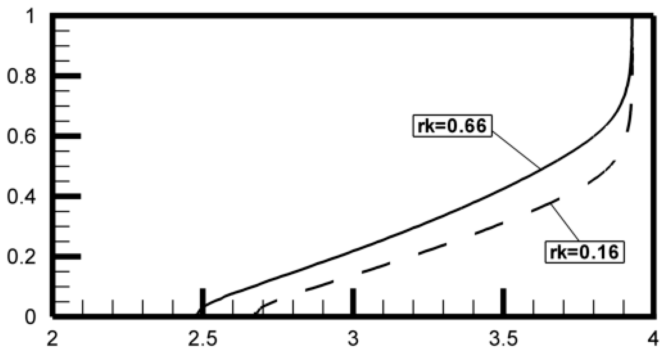
  • Taking advantage of the SA solution, we explained the contradictory results in regard to the effect of anisotropy on the position of the saltwater wedge. We showed that at a constant gravity number, the decrease in the anisotropy ratio leads to landward migration of the saltwater wedge. Contradictions observed in the previous studies are related to the way in which the anisotropy ratio is changed (whether by varying horizontal or vertical hydraulic conductivity). The SA solution shows also that anisotropy leads to a wider mixing zone and intensifies the saltwater flux to the aquifer. It leads to a shallower zone of groundwater discharge to the sea.
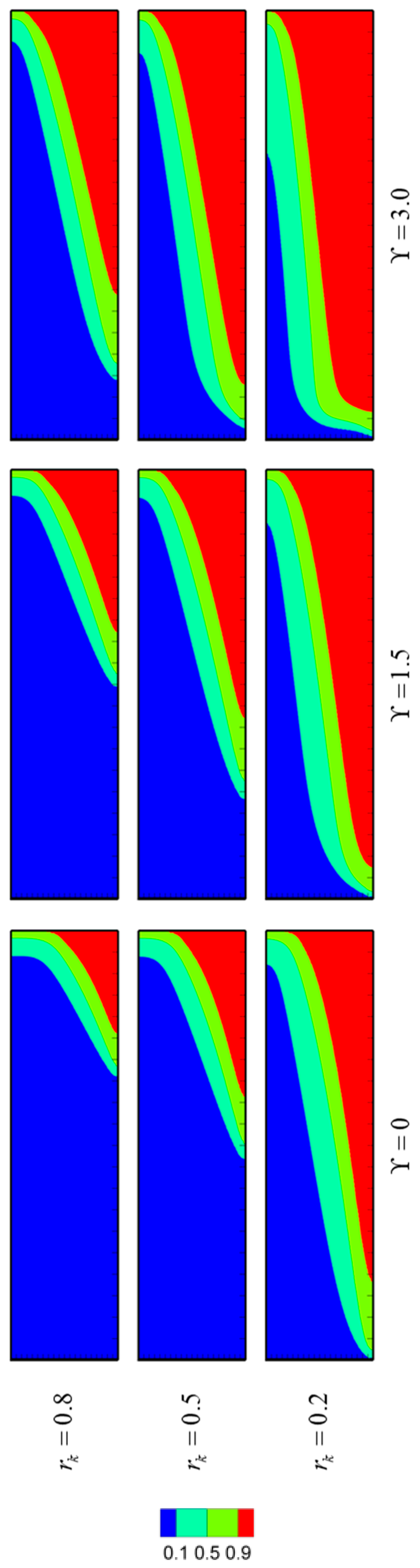
  • The combined effects of anisotropy and stratification on SWI have been investigated. We showed that the width of the mixing zone is slightly sensitive to the rate of stratification. This sensitivity is more significant in highly anisotropic aquifers. Complementary effects of anisotropy and heterogeneity are observed on the saltwater wedge and toe position as well as on the saltwater flux, while opposite effects are observed on the depth of the groundwater discharge zone.
The developed SA solution is limited to vertical seafloor. The salt concentration along the seaside is assumed to be constant. This neglects the effect of freshwater discharge on the saltwater concentration in the discharge zone near the aquifer top surface. Future extensions of this work could include how the SA solution can be used to deal with inclined seafloor and variable saltwater concentration at the sea boundary.

Acknowledgments

Marwan Fahs acknowledges the financial support of the Partenariats Hubert Curien (PHC) via the project CEDRE (35369WE). Behzad Ataie-Ashtiani and Craig T. Simmons acknowledge support from the National Centre for Groundwater Research and Training, Australia. Behzad Ataie-Ashtiani also appreciates the support of the Research office of the Sharif University of Technology, Iran. The FORTRAN source code developed in this study is can be obtained by contacting the corresponding author (Marwan Fahs) at [email protected].

Author Contributions

Behsahd Koohbor worked on the development of the SA solution. Marwan Fahs framed the research questions and finalized the manuscript. Benjamin Belfort worked on the numerical simulations. Behzad Ataie-Ashtiani and Anis Younes supervised the research and analyzed the results. Philippe Ackerer and Craig T. Simmons checked the results and reviewed the manuscript.

Conflicts of Interest

The authors declare no conflict of interest.

Appendix A

Coefficients and matrices for R F and R T
ϖ h 1 = { 2 , i f : h = 0 1 , i f : h 0
B ˜ r , h = { B r , h i f   h N s 0 e l s e
Γ g , r = ( g + r ) 1 ( 1 ) g + r e ϒ ϒ 2 + π 2 ( g + r ) 2 + ( g r ) 1 ( 1 ) g r e ϒ ϒ 2 + π 2 ( g r ) 2
Π g , m = { ( 1 ( 1 ) g + m g + m + 1 ( 1 ) g m g m )    i f   g m 0         i f   g = m
F D i s p is a function representing the dispersion terms. It is given by:
F D i s p = Δ 1 , 1 2 C X 2 + 2 Δ 1 , 2 2 C X Z + Δ 2 , 2 2 C Z 2 + ( C X + 1 ξ ) ( Δ 1 , 1 X + Δ 1 , 2 Z ) + C Z ( Δ 1 , 2 X + Δ 2 , 2 Z )
ϖ g 2 = { 2 i f   g = 0 1 i f   g 0
η g , m , r = δ m + r , g + δ r m , g + δ m r , g
κ g , m , r = δ m + r , g + δ r m , g + δ m r , g
θ h , n , s = ( 1 ) h + n + s 1 h + n + s + ( 1 ) h + n s 1 h + n s + ( 1 ) h n + s 1 h n + s + ( 1 ) h n s 1 h n s
λ h , n , s = ( 1 ) h + n s 1 h + n s + ( 1 ) h n + s 1 h n + s ( 1 ) h + n + s 1 h + n + s ( 1 ) h n s 1 h n s
A ˜ g , n = { A g , n 0 g N m 0 g > N m
Λ g , r = { ( 1 ) g + r 1 g + r + ( 1 ) g r 1 g r i f   g r 0 i f   g = r

References

  1. Henry, H. Effects of dispersion on salt encroachment in coastal aquifer. U.S. Geol. Surv. Water Supply Pap. 1964, 1613, C70–C84. [Google Scholar]
  2. Werner, A.D.; Bakker, M.; Post, V.E.A.; Vandenbohede, A.; Lu, C.; Ataie-Ashtiani, B.; Simmons, C.T.; Barry, D.A. Seawater intrusion processes, investigation and management: Recent advances and future challenges. Adv. Water Resour. 2013, 51, 3–26. [Google Scholar] [CrossRef]
  3. Yang, J.; Graf, T.; Herold, M.; Ptak, T. Modelling the effects of tides and storm surges on coastal aquifers using a coupled surface–subsurface approach. J. Contam. Hydrol. 2013, 149, 61–75. [Google Scholar] [CrossRef] [PubMed]
  4. Grillo, A.; Logashenko, D.; Stichel, S.; Wittum, G. Simulation of density-driven flow in fractured porous media. Adv. Water Resour. 2010, 33, 1494–1507. [Google Scholar] [CrossRef]
  5. Sebben, M.L.; Werner, A.D.; Graf, T. Seawater intrusion in fractured coastal aquifers: A preliminary numerical investigation using a fractured Henry problem. Adv. Water Resour. 2015, 85, 93–108. [Google Scholar] [CrossRef]
  6. Nick, H.M.; Raoof, A.; Centler, F.; Thullner, M.; Regnier, P. Reactive dispersive contaminant transport in coastal aquifers: Numerical simulation of a reactive Henry problem. J. Contam. Hydrol. 2013, 145, 90–104. [Google Scholar] [CrossRef] [PubMed]
  7. Laabidi, E.; Bouhlila, R. Nonstationary porosity evolution in mixing zone in coastal carbonate aquifer using an alternative modeling approach. Environ. Sci. Pollut. Res. 2015, 22, 10070–10082. [Google Scholar] [CrossRef] [PubMed]
  8. Laabidi, E.; Bouhlila, R. Reactive Henry problem: effect of calcite dissolution on seawater intrusion. Environ. Earth Sci. 2016, 75. [Google Scholar] [CrossRef]
  9. Held, R.; Attinger, S.; Kinzelbach, W. Homogenization and effective parameters for the Henry problem in heterogeneous formations. Water Resour. Res. 2005, 41. [Google Scholar] [CrossRef]
  10. Kerrou, J.; Renard, P. A numerical analysis of dimensionality and heterogeneity effects on advective dispersive seawater intrusion processes. Hydrogeol. J. 2010, 18, 55–72. [Google Scholar] [CrossRef]
  11. Alhama Manteca, I.; Alcaraz, M.; Trigueros, E.; Alhama, F. Dimensionless characterization of salt intrusion benchmark scenarios in anisotropic media. Appl. Math. Comput. 2014, 247, 1173–1182. [Google Scholar] [CrossRef]
  12. Qu, W.; Li, H.; Wan, L.; Wang, X.; Jiang, X. Numerical simulations of steady-state salinity distribution and submarine groundwater discharges in homogeneous anisotropic coastal aquifers. Adv. Water Resour. 2014, 74, 318–328. [Google Scholar] [CrossRef]
  13. Abarca, E.; Carrera, J.; Sanchez-Vila, X.; Dentz, M. Anisotropic dispersive Henry problem. Adv. Water Resour. 2007, 30, 913–926. [Google Scholar] [CrossRef]
  14. Mehnert, E.; Jennings, A.A. The effect of salinity-dependent hydraulic conductivity on saltwater intrusion episodes. J. Hydrol. 1985, 80, 283–297. [Google Scholar] [CrossRef]
  15. Walther, M.; Graf, T.; Kolditz, O.; Liedl, R.; Post, V. How significant is the slope of the sea-side boundary for modelling seawater intrusion in coastal aquifers. J. Hydrol. 2017, 551, 648–659. [Google Scholar] [CrossRef]
  16. Sun, D.; Niu, S.; Zang, Y. Impacts of inland boundary conditions on modeling seawater intrusion in coastal aquifers due to sea-level rise. Nat. Hazards 2017, 88, 145–163. [Google Scholar] [CrossRef]
  17. Post, V.E.A.; Vandenbohede, A.; Werner, A.D.; Maimun; Teubner, M.D. Groundwater ages in coastal aquifers. Adv. Water Resour. 2013, 57, 1–11. [Google Scholar] [CrossRef]
  18. Javadi, A.; Hussain, M.; Sherif, M.; Farmani, R. Multi-objective Optimization of Different Management Scenarios to Control Seawater Intrusion in Coastal Aquifers. Water Resour. Manag. 2015, 29, 1843–1857. [Google Scholar] [CrossRef] [Green Version]
  19. Hardyanto, W.; Merkel, B. Introducing probability and uncertainty in groundwater modeling with FEMWATER-LHS. J. Hydrol. 2007, 332, 206–213. [Google Scholar] [CrossRef]
  20. Herckenrath, D.; Langevin, C.D.; Doherty, J. Predictive uncertainty analysis of a saltwater intrusion model using null-space Monte Carlo. Water Resour. Res. 2011, 47. [Google Scholar] [CrossRef]
  21. Rajabi, M.M.; Ataie-Ashtiani, B. Sampling efficiency in Monte Carlo based uncertainty propagation strategies: Application in seawater intrusion simulations. Adv. Water Resour. 2014, 67, 46–64. [Google Scholar] [CrossRef]
  22. Rajabi, M.M.; Ataie-Ashtiani, B.; Janssen, H. Efficiency enhancement of optimized Latin hypercube sampling strategies: Application to Monte Carlo uncertainty analysis and meta-modeling. Adv. Water Resour. 2015, 76, 127–139. [Google Scholar] [CrossRef]
  23. Rajabi, M.M.; Ataie-Ashtiani, B.; Simmons, C.T. Polynomial chaos expansions for uncertainty propagation and moment independent sensitivity analysis of seawater intrusion simulations. J. Hydrol. 2015, 520, 101–122. [Google Scholar] [CrossRef]
  24. Burrows, W.; Doherty, J. Efficient Calibration/Uncertainty Analysis Using Paired Complex/Surrogate Models. Groundwater 2015, 53, 531–541. [Google Scholar] [CrossRef] [PubMed]
  25. Riva, M.; Guadagnini, A.; Dell’Oca, A. Probabilistic assessment of seawater intrusion under multiple sources of uncertainty. Adv. Water Resour. 2015, 75, 93–104. [Google Scholar] [CrossRef]
  26. Sanz, E.; Voss, C.I. Inverse modeling for seawater intrusion in coastal aquifers: Insights about parameter sensitivities, variances, correlations and estimation procedures derived from the Henry problem. Adv. Water Resour. 2006, 29, 439–457. [Google Scholar] [CrossRef]
  27. Carrera, J.; Hidalgo, J.J.; Slooten, L.J.; Vázquez-Suñé, E. Computational and conceptual issues in the calibration of seawater intrusion models. Hydrogeol. J. 2010, 18, 131–145. [Google Scholar] [CrossRef]
  28. Boufadel, M.C.; Suidan, M.T.; Venosa, A.D. A numerical model for density-and-viscosity-dependent flows in two-dimensional variably saturated porous media. J. Contam. Hydrol. 1999, 37, 1–20. [Google Scholar] [CrossRef]
  29. Chen, B.-F.; Hsu, S.-M. Numerical Study of Tidal Effects on Seawater Intrusion in Confined and Unconfined Aquifers by Time-Independent Finite-Difference Method. J. Waterw. Port Coast. Ocean Eng. 2004, 130, 191–206. [Google Scholar] [CrossRef]
  30. Gotovac, H.; Andricevic, R.; Gotovac, B. Multi-resolution adaptive modeling of groundwater flow and transport problems. Adv. Water Resour. 2007, 30, 1105–1126. [Google Scholar] [CrossRef]
  31. Soto Meca, A.; Alhama, F.; González Fernández, C.F. An efficient model for solving density driven groundwater flow problems based on the network simulation method. J. Hydrol. 2007, 339, 39–53. [Google Scholar] [CrossRef]
  32. Younes, A.; Fahs, M.; Ahmed, S. Solving density driven flow problems with efficient spatial discretizations and higher-order time integration methods. Adv. Water Resour. 2009, 32, 340–352. [Google Scholar] [CrossRef]
  33. Servan-Camas, B.; Tsai, F.T.-C. Saltwater intrusion modeling in heterogeneous confined aquifers using two-relaxation-time lattice Boltzmann method. Adv. Water Resour. 2009, 32, 620–631. [Google Scholar] [CrossRef]
  34. Servan-Camas, B.; Tsai, F.T.-C. Two-relaxation-time lattice Boltzmann method for the anisotropic dispersive Henry problem. Water Resour. Res. 2010, 46. [Google Scholar] [CrossRef]
  35. Langevin, C.D.; Dausman, A.M.; Sukop, M.C. Solute and Heat Transport Model of the Henry and Hilleke Laboratory Experiment. Ground Water 2010, 48, 757–770. [Google Scholar] [CrossRef] [PubMed]
  36. Langevin, C.D.; Guo, W. MODFLOW/MT3DMS-Based Simulation of Variable-Density Ground Water Flow and Transport. Ground Water 2006, 44, 339–351. [Google Scholar] [CrossRef] [PubMed]
  37. Pool, M.; Carrera, J.; Dentz, M.; Hidalgo, J.J.; Abarca, E. Vertical average for modeling seawater intrusion. Water Resour. Res. 2011, 47. [Google Scholar] [CrossRef]
  38. Abd-Elhamid, H.F.; Javadi, A.A. A Cost-Effective Method to Control Seawater Intrusion in Coastal Aquifers. Water Resour. Manag. 2011, 25, 2755–2780. [Google Scholar] [CrossRef]
  39. Abd-Elhamid, H.F.; Javadi, A.A. A density-dependant finite element model for analysis of saltwater intrusion in coastal aquifers. J. Hydrol. 2011, 401, 259–271. [Google Scholar] [CrossRef]
  40. Javadi, A.A.; Abd-Elhamid, H.F.; Farmani, R. A simulation-optimization model to control seawater intrusion in coastal aquifers using abstraction/recharge wells. Int. J. Numer. Anal. Methods Geomech. 2012, 36, 1757–1779. [Google Scholar] [CrossRef]
  41. Li, X.; Chen, X.; Hu, B.X.; Navon, I.M. Model reduction of a coupled numerical model using proper orthogonal decomposition. J. Hydrol. 2013, 507, 227–240. [Google Scholar] [CrossRef]
  42. Jamshidzadeh, Z.; Tsai, F.T.-C.; Mirbagheri, S.A.; Ghasemzadeh, H. Fluid dispersion effects on density-driven thermohaline flow and transport in porous media. Adv. Water Resour. 2013, 61, 12–28. [Google Scholar] [CrossRef]
  43. Emami-Meybodi, H.; Hassanzadeh, H. Two-phase convective mixing under a buoyant plume of CO2 in deep saline aquifers. Adv. Water Resour. 2015, 76, 55–71. [Google Scholar] [CrossRef]
  44. Mugunthan, P.; Russell, K.T.; Gong, B.; Riley, M.J.; Chin, A.; McDonald, B.G.; Eastcott, L.J. A Coupled Groundwater-Surface Water Modeling Framework for Simulating Transition Zone Processes. Groundwater 2017, 55, 302–315. [Google Scholar] [CrossRef] [PubMed]
  45. Yoon, S.; Williams, J.R.; Juanes, R.; Kang, P.K. Maximizing the value of pressure data in saline aquifer characterization. Adv. Water Resour. 2017, 109, 14–28. [Google Scholar] [CrossRef]
  46. Ségol, G. Classic Groundwater Simulations: Proving and Improving Numerical Models; Prentice Hall: Upper Saddle River, NJ, USA, 1994; ISBN 978-0-13-137993-0. [Google Scholar]
  47. Diersch, H.-J.G.; Kolditz, O. Variable-density flow and transport in porous media: approaches and challenges. Adv. Water Resour. 2002, 25, 899–944. [Google Scholar] [CrossRef]
  48. Simpson, M.J.; Clement, T.P. Improving the worthiness of the Henry problem as a benchmark for density-dependent groundwater flow models. Water Resour. Res. 2004, 40. [Google Scholar] [CrossRef]
  49. Simpson, M.J.; Clement, T.P. Theoretical analysis of the worthiness of Henry and Elder problems as benchmarks of density-dependent groundwater flow models. Adv. Water Resour. 2003, 26, 17–31. [Google Scholar] [CrossRef]
  50. Weatherill, D.; Simmons, C.T.; Voss, C.I.; Robinson, N.I. Testing density-dependent groundwater models: two-dimensional steady state unstable convection in infinite, finite and inclined porous layers. Adv. Water Resour. 2004, 27, 547–562. [Google Scholar] [CrossRef]
  51. Prasad, A.; Simmons, C.T. Using quantitative indicators to evaluate results from variable-density groundwater flow models. Hydrogeol. J. 2005, 13, 905–914. [Google Scholar] [CrossRef]
  52. Goswami, R.R.; Clement, T.P. Laboratory-scale investigation of saltwater intrusion dynamics. Water Resour. Res. 2007, 43. [Google Scholar] [CrossRef]
  53. Voss, C.I.; Simmons, C.T.; Robinson, N.I. Three-dimensional benchmark for variable-density flow and transport simulation: matching semi-analytic stability modes for steady unstable convection in an inclined porous box. Hydrogeol. J. 2010, 18, 5–23. [Google Scholar] [CrossRef]
  54. Younes, A.; Fahs, M. A semi-analytical solution for saltwater intrusion with a very narrow transition zone. Hydrogeol. J. 2014, 22, 501–506. [Google Scholar] [CrossRef]
  55. Zidane, A.; Younes, A.; Huggenberger, P.; Zechner, E. The Henry semianalytical solution for saltwater intrusion with reduced dispersion. Water Resour. Res. 2012, 48. [Google Scholar] [CrossRef]
  56. Chang, S.W.; Clement, T.P.; Simpson, M.J.; Lee, K.-K. Does sea-level rise have an impact on saltwater intrusion. Adv. Water Resour. 2011, 34, 1283–1291. [Google Scholar] [CrossRef] [Green Version]
  57. Fahs, M.; Ataie-Ashtiani, B.; Younes, A.; Simmons, C.T.; Ackerer, P. The Henry problem: New semianalytical solution for velocity-dependent dispersion. Water Resour. Res. 2016, 52, 7382–7407. [Google Scholar] [CrossRef]
  58. Michael, H.A.; Russoniello, C.J.; Byron, L.A. Global assessment of vulnerability to sea-level rise in topography-limited and recharge-limited coastal groundwater systems. Water Resour. Res. 2013, 49, 2228–2240. [Google Scholar] [CrossRef]
  59. Simmons, C.T.; Fenstemaker, T.R.; Sharp, J.M. Variable-density groundwater flow and solute transport in heterogeneous porous media: Approaches, resolutions and future challenges. J. Contam. Hydrol. 2001, 52, 245–275. [Google Scholar] [CrossRef]
  60. Chang, C.-M.; Yeh, H.-D. Spectral approach to seawater intrusion in heterogeneous coastal aquifers. Hydrol. Earth Syst. Sci. 2010, 14, 719–727. [Google Scholar] [CrossRef]
  61. Lu, C.; Chen, Y.; Zhang, C.; Luo, J. Steady-state freshwater–seawater mixing zone in stratified coastal aquifers. J. Hydrol. 2013, 505, 24–34. [Google Scholar] [CrossRef]
  62. BniLam, N.; Al-Khoury, R. A spectral element model for nonhomogeneous heat flow in shallow geothermal systems. Int. J. Heat Mass Transf. 2017, 104, 703–717. [Google Scholar] [CrossRef]
  63. Gardner, W.R. Some Steady-state solutions of the unsaturated moisture flow equation with application to evaporation from water table. Soil Sci. 1958, 85, 228. [Google Scholar] [CrossRef]
  64. Fajraoui, N.; Fahs, M.; Younes, A.; Sudret, B. Analyzing natural convection in porous enclosure with polynomial chaos expansions: Effect of thermal dispersion, anisotropic permeability and heterogeneity. Int. J. Heat Mass Transf. 2017, 115, 205–224. [Google Scholar] [CrossRef]
  65. Wang, X.-S.; Jiang, X.-W.; Wan, L.; Ge, S.; Li, H. A new analytical solution of topography-driven flow in a drainage basin with depth-dependent anisotropy of permeability. Water Resour. Res. 2011, 47. [Google Scholar] [CrossRef]
  66. Jiang, X.-W.; Wan, L.; Wang, X.-S.; Ge, S.; Liu, J. Effect of exponential decay in hydraulic conductivity with depth on regional groundwater flow. Geophys. Res. Lett. 2009, 36. [Google Scholar] [CrossRef]
  67. Kuang, X.; Jiao, J.J. An integrated permeability-depth model for Earth’s crust: Permeability of Earth’s crust. Geophys. Res. Lett. 2014, 41, 7539–7545. [Google Scholar] [CrossRef]
  68. Zlotnik, V.A.; Cardenas, M.B.; Toundykov, D. Effects of Multiscale Anisotropy on Basin and Hyporheic Groundwater Flow. Ground Water 2011, 49, 576–583. [Google Scholar] [CrossRef] [PubMed]
  69. Younes, A.; Fahs, M. Extension of the Henry semi-analytical solution for saltwater intrusion in stratified domains. Comput. Geosci. 2015, 19, 1207–1217. [Google Scholar] [CrossRef]
  70. Ghezzehei, T.A.; Kneafsey, T.J.; Su, G.W. Correspondence of the Gardner and van Genuchten-Mualem relative permeability function parameters. Water Resour. Res. 2007, 43. [Google Scholar] [CrossRef]
  71. Fahs, M.; Younes, A.; Mara, T.A. A new benchmark semi-analytical solution for density-driven flow in porous media. Adv. Water Resour. 2014, 70, 24–35. [Google Scholar] [CrossRef]
  72. Pool, M.; Post, V.E.A.; Simmons, C.T. Effects of tidal fluctuations and spatial heterogeneity on mixing and spreading in spatially heterogeneous coastal aquifers. Water Resour. Res. 2015, 51, 1570–1585. [Google Scholar] [CrossRef]
  73. Houben, G.J.; Stoeckl, L.; Mariner, K.E.; Choudhury, A.S. The influence of heterogeneity on coastal groundwater flow-physical and numerical modeling of fringing reefs, dykes and structured conductivity fields. Adv. Water Resour. 2017, 113, 155–166. [Google Scholar] [CrossRef]
  74. Dose, E.J.; Stoeckl, L.; Houben, G.J.; Vacher, H.L.; Vassolo, S.; Dietrich, J.; Himmelsbach, T. Experiments and modeling of freshwater lenses in layered aquifers: Steady state interface geometry. J. Hydrol. 2014, 509, 621–630. [Google Scholar] [CrossRef]
  75. Guevara Morel, C.R.; van Reeuwijk, M.; Graf, T. Systematic investigation of non-Boussinesq effects in variable-density groundwater flow simulations. J. Contam. Hydrol. 2015, 183, 82–98. [Google Scholar] [CrossRef] [PubMed]
  76. Huyakorn, P.S.; Andersen, P.F.; Mercer, J.W.; White, H.O. Saltwater intrusion in aquifers: Development and testing of a three-dimensional finite element model. Water Resour. Res. 1987, 23, 293–312. [Google Scholar] [CrossRef]
  77. Mehdizadeh, S.S.; Werner, A.D.; Vafaie, F.; Badaruddin, S. Vertical leakage in sharp-interface seawater intrusion models of layered coastal aquifers. J. Hydrol. 2014, 519, 1097–1107. [Google Scholar] [CrossRef]
  78. Najib, K.; Rosier, C. On the global existence for a degenerate elliptic–parabolic seawater intrusion problem. Math. Comput. Simul 2011, 81, 2282–2295. [Google Scholar] [CrossRef]
  79. Felisa, G.; Ciriello, V.; Federico, V. Saltwater Intrusion in Coastal Aquifers: A Primary Case Study along the Adriatic Coast Investigated within a Probabilistic Framework. Water 2013, 5, 1830–1847. [Google Scholar] [CrossRef]
  80. Marion, P.; Najib, K.; Rosier, C. Numerical simulations for a seawater intrusion problem in a free aquifer. Appl. Numer. Math. 2014, 75, 48–60. [Google Scholar] [CrossRef]
  81. Masciopinto, C.; Liso, I.; Caputo, M.; De Carlo, L. An Integrated Approach Based on Numerical Modelling and Geophysical Survey to Map Groundwater Salinity in Fractured Coastal Aquifers. Water 2017, 9, 875. [Google Scholar] [CrossRef]
  82. Essaid, H.I. A multilayered sharp interface model of coupled freshwater and saltwater flow in coastal systems: Model development and application. Water Resour. Res. 1990, 26, 1431–1454. [Google Scholar] [CrossRef]
  83. Pistiner, A.; Shapiro, M. A model for a moving interface in a layered coastal aquifer. Water Resour. Res. 1993, 29, 329–340. [Google Scholar] [CrossRef]
  84. Dagan, G.; Zeitoun, D.G. Seawater-freshwater interface in a stratified aquifer of random permeability distribution. J. Contam. Hydrol. 1998, 29, 185–203. [Google Scholar] [CrossRef]
  85. Liu, Y.; Mao, X.; Chen, J.; Barry, D.A. Influence of a coarse interlayer on seawater intrusion and contaminant migration in coastal aquifers. Hydrol. Process. 2014, 28, 5162–5175. [Google Scholar] [CrossRef]
  86. Qin, R.; Wu, Y.; Xu, Z.; Xie, D.; Zhang, C. Numerical modeling of contaminant transport in a stratified heterogeneous aquifer with dipping anisotropy. Hydrogeol. J. 2013, 21, 1235–1246. [Google Scholar] [CrossRef]
  87. Woumeni, R.S.; Vauclin, M. A field study of the coupled effects of aquifer stratification, fluid density, and groundwater fluctuations on dispersivity assessments. Adv. Water Resour. 2006, 29, 1037–1055. [Google Scholar] [CrossRef]
Figure 1. The Henry problem (HP) assumptions (a) real configuration and (b) conceptual model [3].
Water 10 00230 g001
Figure 2. Variation of the horizontal and vertical hydraulic conductivities with respect to depth for ϒ = 1.5 and K z ¯ = 8.213 × 10 3   m / s . Depth datum is at the aquifer bottom surface.
Water 10 00230 g002
Figure 3. Non-physical oscillations related to the Gibbs phenomenon: the heterogeneous pure diffusive case evaluated with insufficient number of Fourier modes.
Water 10 00230 g003
Figure 4. Semi-analytical and numerical isochlors (10%, 50% and 90%) for the pure diffusive cases: (a) homogenous and (b) heterogonous aquifer.
Water 10 00230 g004
Figure 5. Semi-analytical and numerical isochlors (10%, 50%, 90%) for the dispersive cases: (a) homogenous and (b) heterogonous aquifer.
Water 10 00230 g005
Figure 6. Effect of anisotropy on the isochlors’ positions (90%, 50%, 10%): Results obtained for the dispersive homogenous case (see Table 1 for all parameters, except r K , which is given in the figure).
Water 10 00230 g006
Figure 7. Effect of anisotropy ratio on the 50% isochlor’s position when r K is changed based on the vertical hydraulic conductivity. The case r K = 0.66 corresponds to the homogenous dispersive case (Table 2). The case r K = 0.16 is obtained with reduced K z (divided by 4.125).
Water 10 00230 g007
Figure 8. Variation of the SWI metrics ((a) L t o e , (b) W M Z , (c) Q s and (d) d d i s c h ) versus r k . Results obtained for the dispersive case (see Table 1 for all parameters, except r K and ϒ , which are given in the figure).
Water 10 00230 g008
Figure 9. Coupled influence of anisotropy and heterogeneity on the main isochlors (10%, 50%, 90%). Results obtained for a fixed large-scale gravity number N G ¯ = 3.11 . All other parameters are similar to the dispersive case in Table 1.
Water 10 00230 g009
Figure 10. Effect of the heterogeneity for a varying large-scale gravity number. The 50% isochlor in the case of the homogenous aquifer with N G ¯ = 3.11 (solid line), heterogeneous aquifer with N G ¯ = 3.11 (dashed line) and heterogeneous aquifer with N G ¯ = 0.84 (dash-dotted line). Heterogeneous cases are obtained with ϒ = 1.5 .
Water 10 00230 g010
Table 1. Non-dimensional parameters used in the semi-analytical solution for the verification test cases.
Dimensionless ParametersValueCases
N G ¯ = K z ¯ d Δ ρ ρ 0 q d . 3.11All cases
b m = ε D m / q d 0.1
5 × 10⁻⁴
Diffusive cases
Dispersive cases
Non-dimensional longitudinal dispersion b L = α L / d 0
0.1
Diffusive cases
Dispersive cases
Transverse to longitudinal dispersion coefficients ratio r α = α T / α L 0
0.1
Diffusive cases
Dispersive cases
r K = K z / K x 0.66All cases
The rate of heterogeneity ϒ 0
1.5
Homogenous cases
Heterogeneous cases
Table 2. Physical parameters used in the numerical model for the verification test cases.
ParametersValueCases
Δ ρ [kg/m3]25All cases
ρ 0 [kg/m3]1000All cases
q d [m2/s]6.6 × 10−5All cases
d [m]1All cases
[m]4All cases
K z ¯ [m/s]8.213 × 10−3All cases
r k [-]0.66All cases
ε [-]0.35All cases
D m [m2/s]53.88 × 10−6
3.300 × 10⁻⁸
Diffusive cases
Dispersive cases
α L [m]0
0.1
Diffusive cases
Dispersive cases
α T [m]0
0.01
Diffusive cases
Dispersive cases
ϒ [-]0
1.5
Homogenous cases
Heterogeneous cases
Table 3. Physical parameters used in the numerical model for the verification test cases (Ltoe: length of the toe, WMZ: average vertical width of the mixing zone, QS: total dimensionless salt flux, ddisch: depth of the zone of groundwater discharge to the sea).
Semi-Analytical SolutionNumerical Solution
Metrics L t o e W M Z Q s d d i s c h L t o e W M Z Q s d d i s c h
Diffusive homogenous0.740.781.060.570.740.791.090.56
Diffusive heterogeneous0.950.831.090.350.950.841.010.36
Dispersive homogenous1.540.291.070.461.530.291.090.47
Dispersive heterogeneous2.300.591.090.312.290.591.120.31

