Extracting Farmland Features from Lidar-Derived DEM for Improving Flood Plain Delineation

1
Department of Geographic Information Science, Nanjing University, Nanjing 210023, China
2
Changjiang River Scientific Research Institute, Changjiang Water Resources Commission, Wuhan 430010, China
3
Department of Surveying and Mapping Engineering, Datong University, 037009 Datong, China
4
Jiangsu Center for Collaborative Innovation in Geographical Information Resource Development and Application, Nanjing 210023, China
*
Author to whom correspondence should be addressed.
Water 2018, 10(3), 252; https://doi.org/10.3390/w10030252
Submission received: 6 December 2017
/
Revised: 16 February 2018
/
Accepted: 22 February 2018
/
Published: 1 March 2018
(This article belongs to the Special Issue Assessment of Current and Future Vulnerability of Flooding with Hydrologic/Hydraulic Modeling and Remote Sensing Techniques)
Abstract
:Flood plains, which are commonly distributed in flat river or lake basins, often contain large tracts of farmland. Therefore, flood plains require precise and detailed information on the role played by farmland in flood routing simulations, flood risk evaluation, and flood loss evaluation. In farmland, cultivated land parcels are not directly adjacent. The intervening non-cultivable land, which might include trails and ditches, can cover large areas. Currently, the area of non-cultivable land between cultivated land parcels is usually measured by artificial visual interpretation or by fieldwork. This study focused on the extraction of uncultivable trails, ditches, and cultivated field parcels within farmland on the basis of a Light Detection and Ranging-derived (LiDAR-derived) high-resolution gridded Digital Elevation Model (DEM). The proposed approach was applied to generate polygons of individual land parcels in a flood storage and detention area. The DEM was first smoothed and then subtracted. To remove small spots and to smooth the boundaries of the land parcels, inner and outer buffers were created to generalize the extracted polygons. Experiments proved that this approach is applicable in flood plain farmland and demonstrated that the chosen parameters were appropriate. This approach is more efficient than traditional surveying methods. For field parcel extraction, the accuracy achieved was 93.42%, using official statistics for comparison, and the Cohen’s kappa coefficient was 0.90, using a visual interpretation of an aerial image for comparison. The kappa coefficients were 0.87 and 0.77 for trail and ditch extraction, respectively.
1. Introduction
Flooding is one of the most serious natural disasters, putting lives at risk and causing damage to buildings and other infrastructure. Flood plains are flat areas of land next to rivers or lakes; they are usually rural. Farmland cover large tracts of flood plains and can be inundated by floodwaters, which prevents crops from being harvested. The loss of harvests can sometimes lead to long-term effects even after floodwaters recede. On flood plains, precise and detailed disaster-forming and -affected information for farmland is a basic data source for flood simulation, flood-loss evaluation, and flood risk evaluation [1]. The disaster-forming environment can affect the distribution of flooding; meanwhile, changes to flooding can affect disaster-affected bodies. It is relevant to the surface roughness of 2D flood routing simulations, the generation of computational meshes in high-resolution flood simulations, and the prediction of crop yield and flood loss. For flood plains with special flood risk, flood risk analysis is characterized by a small scale and a high precision, in particular, requiring a focus on the effects of various small-scale features [2]. One of the most basic tasks is to obtain accurate and reliable land use data.
Generally, parcels of farmland are not immediately adjacent but are separated by trails and ditches. Even small differences in the areas of such intervening spaces could lead to significant differences in calculations of the flood processes, flood risk and loss of land [3]. Therefore, detailed measurements of farmland resources provide disaster-forming and -affected information that is important for the development of efficient farmland flood research methods.
Generally, the trails and ditches between parcels of cultivated land, many of which might only be 1–2 m wide, are too small to be represented on small-scale maps. However, on large-scale maps, such objects are important and cannot be neglected, particularly for precise assessments of flood risk and loss.
In existing widely used surveying techniques, areas of non-cultivable land are generally assessed by fieldwork, which can be costly and time consuming. Often, such areas are not all measured individually. Instead, sample areas are chosen and assessed to obtain a representative ratio of cultivable/non-cultivable land. This strategy can reduce both time and cost overheads, but it also increases the risk of uncertainty. In this research, ditches and trails crossing farmland as well as cultivated fields were extracted from an airborne LiDAR-derived high-resolution DEM, which provided results with improved accuracy at less cost.
Satellite imagery and DEMs have already been incorporated into land-surveying methods [4,5]. The Global Land Survey (GLS) datasets provided by the United States Geological Survey (USGS) and National Aeronautics and Space Administration (NASA), which consist of near-global coverage of the land area obtained every 10 years since the early 1970s, have been widely used in land-surveying studies [6]. However, for small-scale studies, land parcels have usually had to be mapped by visual interpretation, which is imprecise and costly. Therefore, some researchers have explored possibilities for using object-oriented methods to extract small-scale land parcels [7,8].
LiDAR provides high-resolution topographic data that have promoted the development of new approaches in the extraction of land parcel information. LiDAR collects elevation data of several surface levels with intensity information of every return. The first returns are used to generate digital surface models (DSMs), and the last returns are used for the generation of digital terrain models (DTMs) [9]. For its ability of penetration and accuracy, LiDAR is valuable in landform analyses such as landslide detection [10], glacial mapping [11], forestry [12], habitat analysis [13], and so on.
Few studies have focused on the extraction of trails in farmland. Some forest trails have been extracted by detecting corridors in near- or above-ground vegetation points according to the spatial structure or intensity of point clouds [14,15]; however, it seems to be a different situation in farmland. Trails in farmland are almost bare earth partly covered by grass, and thus the characteristics that make forest trails unique are not reliable and depend on the growth stage of crops. For water conservation, trails in farmland appear convex on the surface; some research has been conducted on other ground features that have similar shapes (e.g., levees, ridges, and peaks). For example, slopes calculated using LiDAR data were used to extract four geometric parameters of levees on the Sacramento River in the United States [16] and levee lines in the Nakdong River Basin in South Korea [17]. Another study used the least-cost path analysis, matrix, perpendicular line and matched points transecting methods to extract levee-crest elevation profiles in southern Louisiana in the United States [18].
Ridges are continuous elevated crests of mountains, and although they are much bigger than trails within farmland areas, they exhibit some similar characteristics. The steepest ascent and discrete Laplace transform methods are widely used in ridge detection [19,20]. However, research has investigated the use of morphometric parameters and a new classification scheme to characterize several types of landforms, including ridges [21]. Hydrological methods have also been introduced to ridge and peak detection by reversing DEM data [22].
Although the methods mentioned above have performed well in levee or ridge detection, their efficiency in extracting trails in farmland has yet to be proven. Trails are generally much smaller in size than both levees and ridges, and they are present on an artificial surface; thus, they have specific characteristics.
A large number of publications have proposed methods for extracting water systems from gridded DEM, Triangulated Irregular Network (TIN), or contour data; among these, gridded DEMs are the most widely used. There are two basic approaches when using a gridded DEM: a topographic surface analysis method and a physical water model method. Topographic surface analysis methods can only obtain characteristic lines and are often case specific. Physical water model methods are often found to be unsuitable for applications in plain areas [23,24], particularly those with manual canal and ditch systems.
This paper proposes a method for the extraction of cultivated fields, trails, and ditches in farmland areas. An airborne LiDAR-derived high-resolution DEM was used to present detailed shapes of small trails and ditches. The method was employed in a flood storage and detention area, and the accuracy of the generated land parcels was assessed.
2. Research Area and Data
2.1. Research Area
To test the effectiveness of the proposed method in obtaining farmland objects for flood research, a flood storage and detention area was selected.
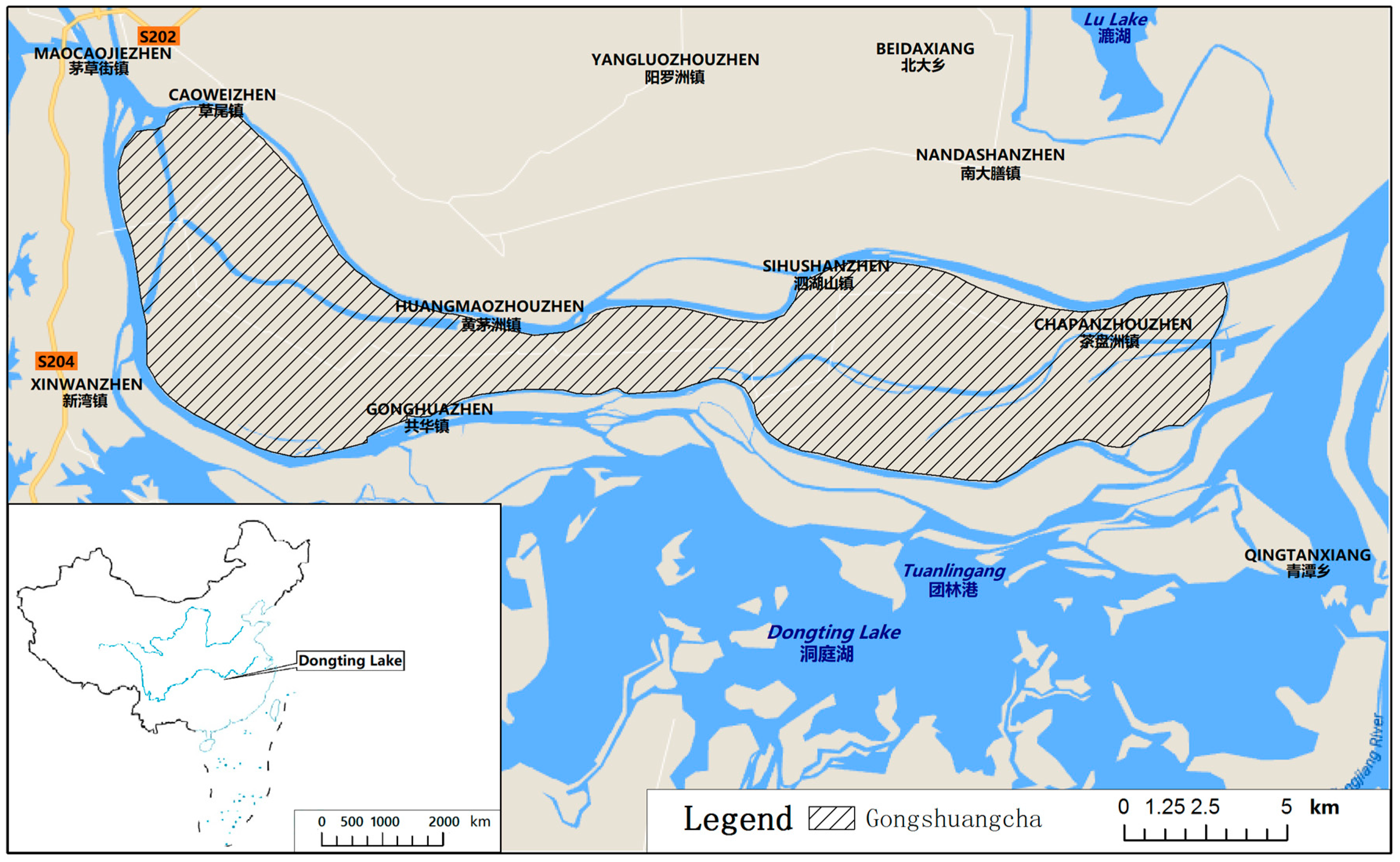
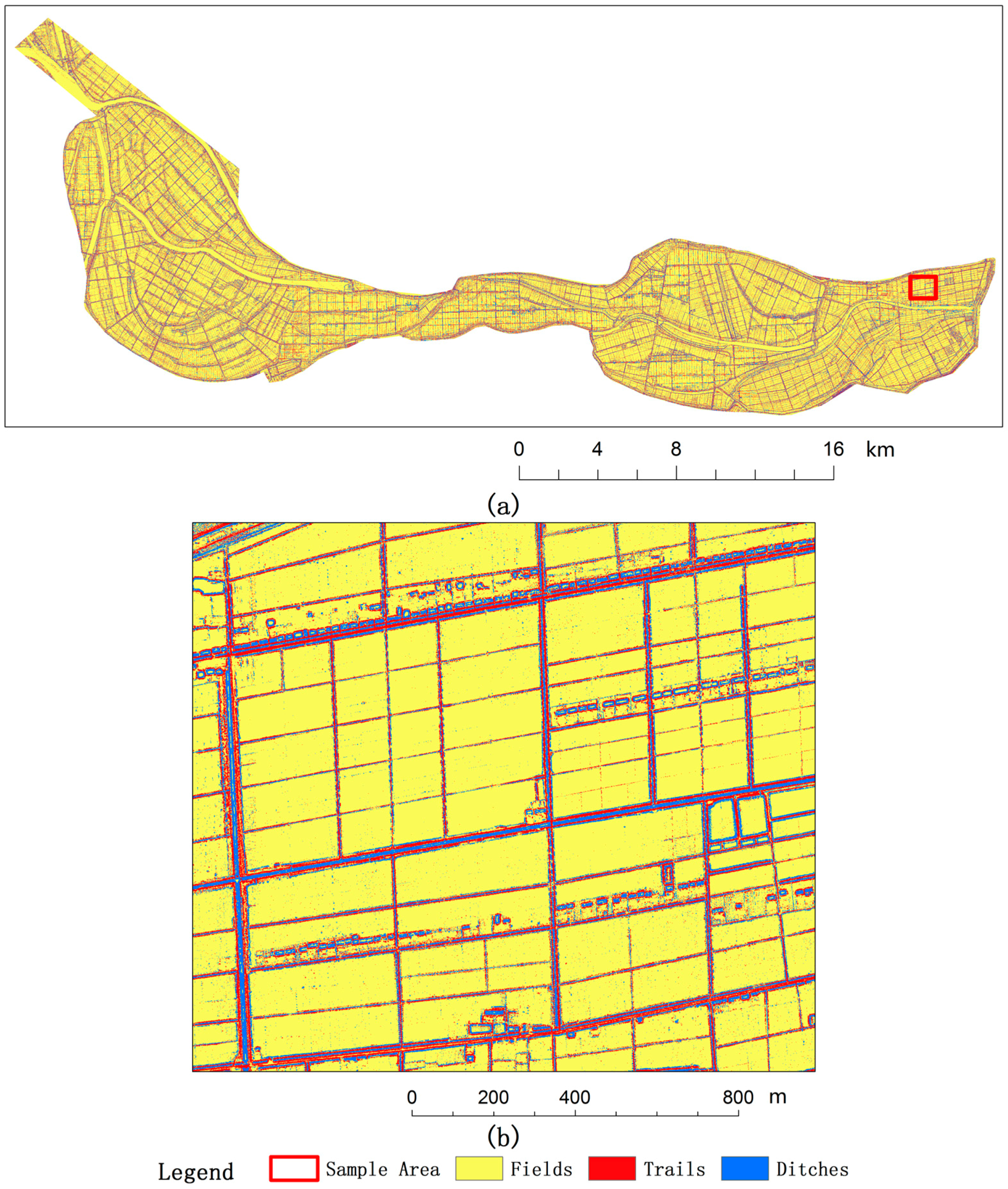
The research area was located in Gongshuangcha, a flood plain in the Dongting Lake area, which is near Yuanjiang in Hunan Province, China (Figure 1). Dongting Lake is one of the main impounded lakes of the Yangtze River. Owing to frequent rainstorms, the Dongting Lake area is prone to floods. From the 1950s to the 1970s, it flooded every 5 years; in the 1980s, it flooded every 3 to 4 years; in the 1990s, it even flooded every 1 to 2 years [25,26]. So far, there are over 3471 km of dikes in the Dongting Lake area [25]. Diking has placed a heavy burden on the region’s socioeconomic development.
As a flood storage and detention area, it is mainly a plain landscape formed by river and lake sediments, with low-lying flat open fields criss-crossed by trails and ditches. This area consists mainly of embankments, which are a common land use type in the Dongting Lake area, where lake-silted areas are protected by surrounding levees. Therefore, farmland parcels, canals, and trails constitute most of the ground objects within this area. The main crop cultivated in this region is rice.
2.2. Data
An airborne LiDAR-derived high-resolution DEM of the research area was used. The LiDAR point cloud was obtained in December 2010, when Gongshuangcha was in winter and in its dry season. Rice had been harvested at that time of the year. The camera was a Rollei (Braunschweig, Germany) Metric AIC Pro and the laser scanner was a Reigl (Horn, Austria) LMS-Q680i. More parameters are listed in Table 1 and Table 2. The flying altitude was 1300 m, and the point density was approximately 1–2 points/m2.
The LiDAR point cloud included ground points, vegetation points, building points, noise points, and so on. Filtering was applied to separate ground points and non-ground points. A gridded DEM was established after ground points in the LiDAR point cloud were filtered. The DEM’s horizontal resolution was 1 m with 51,000 × 22,000 pixels. The lowest elevation in the DEM was 4.55 m, and the highest was 45.87 m. Over the whole research area, the elevation difference was only 41.32 m. Figure 2 illustrates the DEM of the Gongshuangcha research area.
3. Methodology
Ditches are artificial channels distributed through fields for irrigation and drainage, whereas trails are raised paths through fields, which are used for access and for water conservation; together they form concave and convex belts running through areas of farmland (Figure 3). Many trails in the research area acted as small levees between cultivated fields and ditches. In Gongshuangcha, most of the ditches and trails through the farmland are no wider than 2 m.
In this study, the surface was first smoothed to remove concave or convex parts, including ditches, trails, some small peaks, and pits. Then, the original surface was subtracted from the smoothed surface to detect the convex, concave, and flat parts. The three parts were converted into polygons, and then spots such as peaks or pits were removed to generate trail, ditch, and field polygons. Trails were extracted by detecting convexity, ditches were extracted by detecting concavity, and fields were extracted by detecting flatness. By smoothing, an overall terrain was obtained; the original DEM contained all the detailed farmland micro-terrain. Comparing the overall terrain and the micro-terrain, farmland features could be detected.
3.1. Smoothing
To smooth the surface, the mean value of the elevation within a neighborhood around each pixel was used to replace its original value. Therefore, pixels in convex or concave parts were reduced or raised to be close to those in flat parts. After surface smoothing, only the very basic features of the terrain and objects were retained (Figure 4).
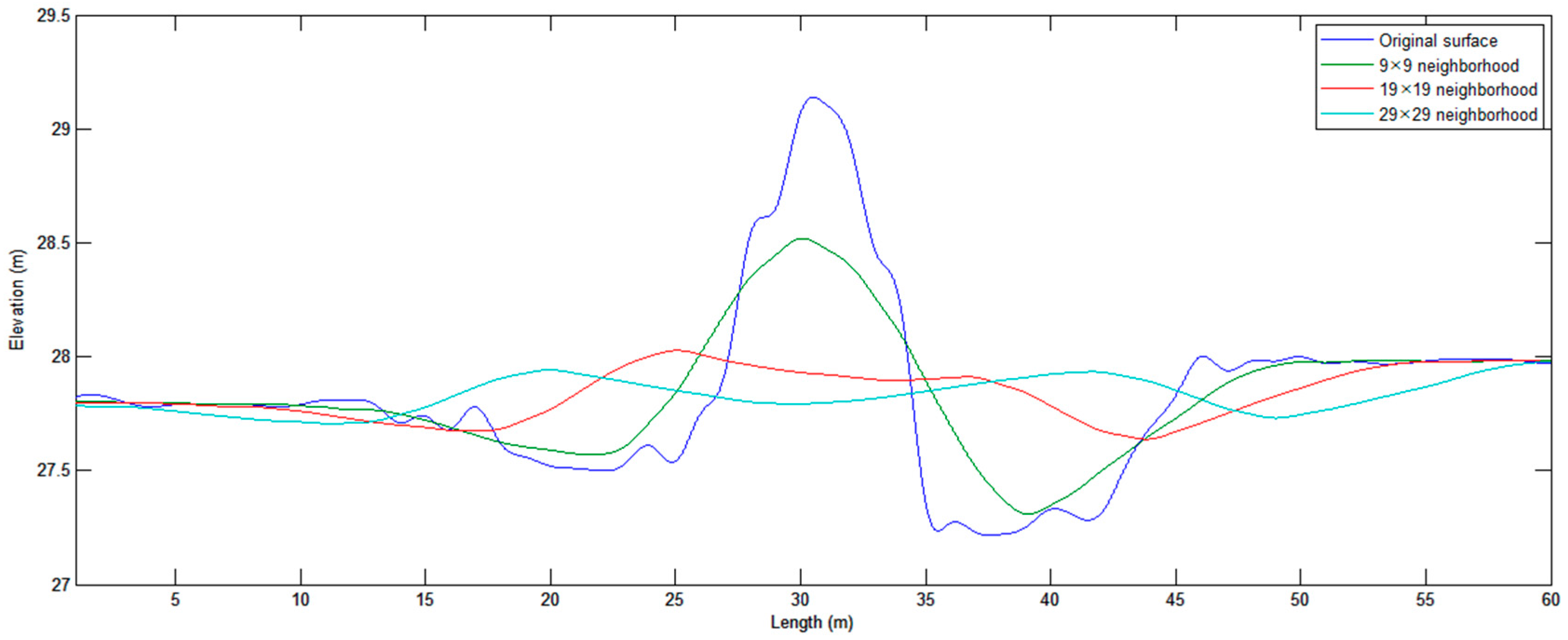
The size of a neighborhood could affect the smoothing results. For example, the navy blue line in Figure 5 represents the original surface of a section of farmland with a trail in the research area. After smoothing using a 9 × 9 m neighborhood square, the trail continued to protrude on the smoothed surface (green line in Figure 5). Surfaces smoothed using 19 × 19 m and 29 × 29 m neighborhood squares are represented by the pink and light-blue lines, respectively, in Figure 5. It is evident that the larger the neighborhood size, the lower the elevation of the smoothed trail and the flatter the smoothed surface.
Clearly, convex parts were smoothed more when larger neighborhoods were used. However, if the neighborhood was much larger than the objects targeted in the smoothing process, other large convex ridges such as high roads or levees would also be smoothed, which was undesirable. Thus, on the basis of how neighborhood size affected the smoothing results, the optimum neighborhood size depended on the sizes of the target objects.
Irrespective of the neighborhood size, there would always be a “top” on a smoothed trail or a “bottom” on a smoothed ditch. When the top or the bottom was sufficiently masked, the smoothing results could be considered acceptable. We let be the width of a trail or ditch, be the height relative to the areas on both its sides, and be the length of a side of the neighborhood. The height of the top or bottom of the smoothed trail or ditch could be determined as . In this study, most of the trails and ditches were no more than 1 m higher or deeper than the areas on either side of them; therefore, was no more than m. Thus, a square with sides 3 times the width of a trail was chosen as the neighborhood in this study. The value of was no more than m, which was sufficiently masked for it to be considered a flat surface. For this research area, which was flat and had many small trails and ditches, a 6 m square was chosen as the neighborhood size.
3.2. Detecting Features by Subtraction
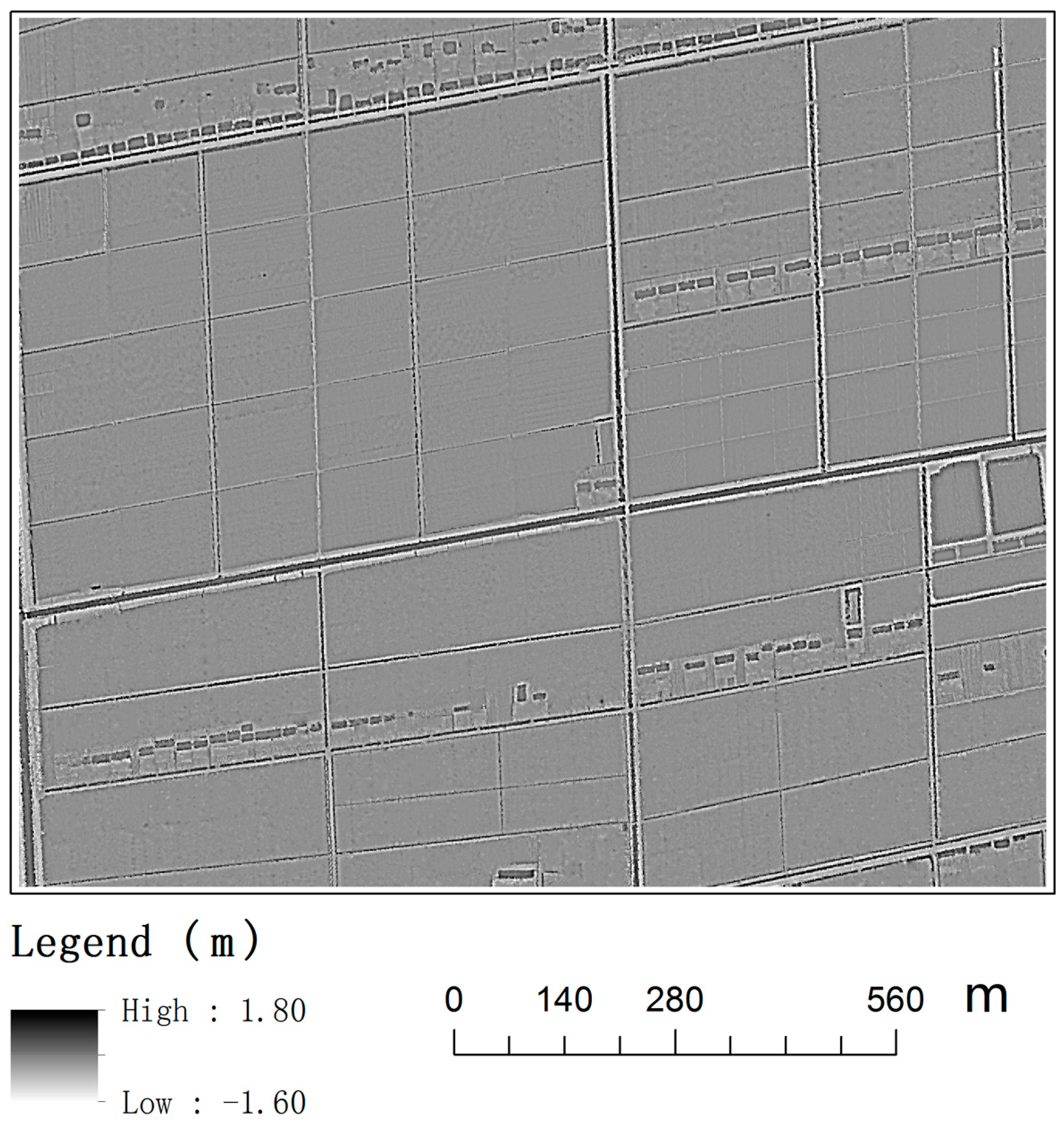
After smoothing the entire surface, the original surface was subtracted from the smoothed surface to generate a new surface. On this new surface, a pixel with a negative value (i.e., smoothed elevation lower than the original elevation) was more likely in convex parts, a pixel with a positive value was more likely in concave parts, and a pixel with a zero value was more likely in flat parts. Thus, the new surface was divided into three classes: a pixel with a sufficiently low negative value could be chosen as a “trail candidate”, a pixel with a sufficiently high positive value could be chosen as a “ditch candidate”, and a pixel with a value around zero could be chosen as a “field candidate”. As mentioned above, when a square with sides 3 times the width of the trails and ditches was chosen as the neighborhood size, most trails would be no more than m on the smoothed surface, and most ditches would be no less than m. Thus, in this study, a pixel with a value lower than m was recognized as a trail candidate, a pixel with a value higher than m was recognized as a ditch candidate, and a pixel with a value between and m was recognized as a field candidate. On the new surface (Figure 6), white lines indicate the locations of trails, and the dark lines indicate the locations of ditches.
3.3. Generalizing Polygons
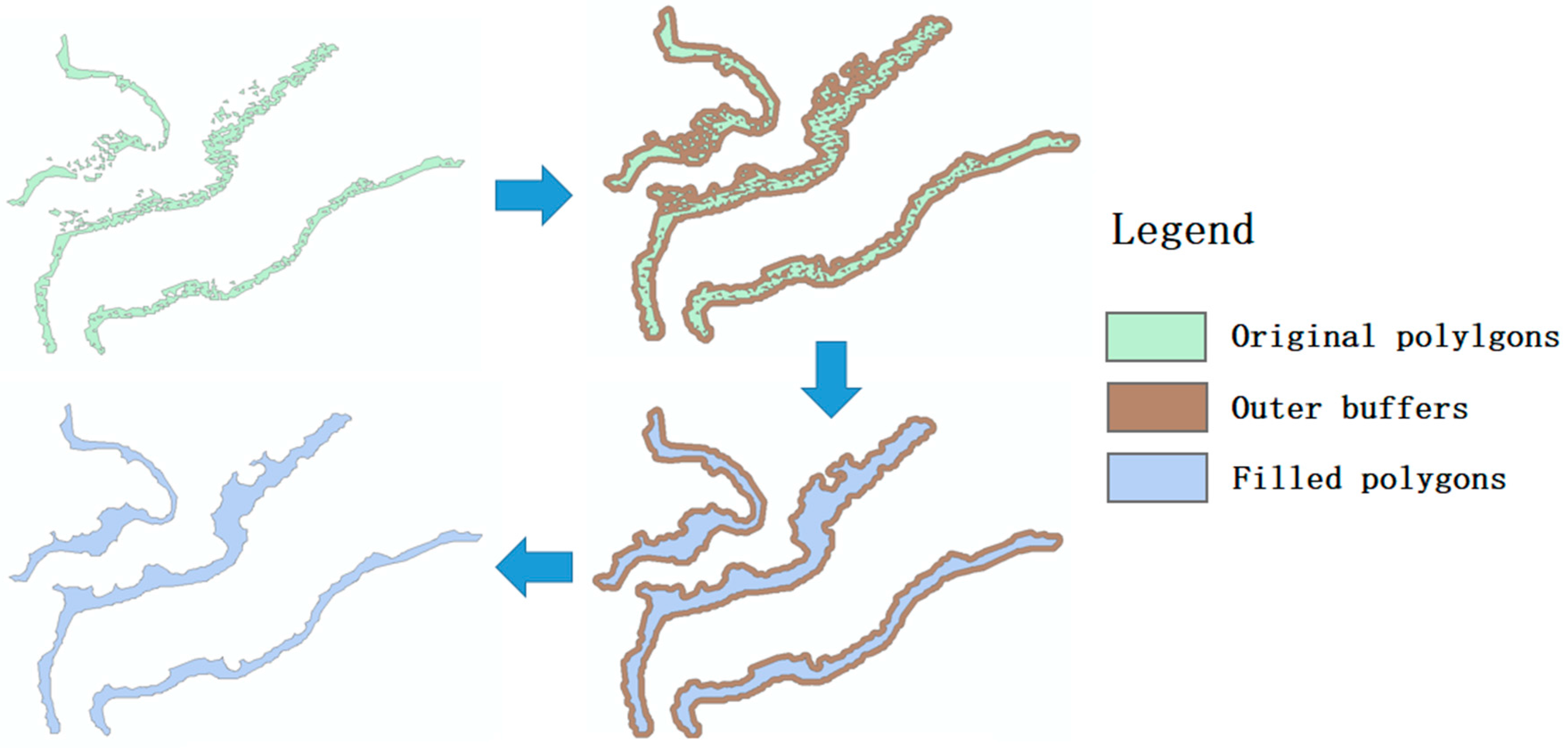
Using the results from the subtraction, the polygons were generalized. First, the trail candidate, ditch candidate and field candidate pixels were converted into polygons separately. However, high-precision data provided not only detailed ground information, but also additional noise. Thus, convex parts could have been trails but also could have been small peaks. Similarly, concave parts could have been ditches but also could have been small pits. Therefore, the polygons had to be generalized to make them more sensible. Fortunately, unlike peaks or pits, trails and ditches are continuous ribbon-like features, and field parcels are whole blocky pieces; thus, small peaks and pits could be eliminated by removing dispersed polygons. In this study, to remove holes in a polygon caused by peaks or pits, an outer buffer was made first to fill the holes; then an inner buffer with the same distance was made (Figure 7). Similarly, an inner buffer was made first to erode dispersed polygons; then an outer buffer with the same distance was made to restore the other polygons (Figure 8). However, if the buffer distances were too wide, some continuous polygons would have been eroded in addition to the dispersed polygons (Figure 8a). To eliminate most peaks and pits, and to ensure no trails or ditches were eroded or filled, a value of half the width of the trails and ditches was chosen as the buffer distance, which, for this case in Gongshuangcha, was 1 m.
4. Results and Discussion
An experiment on the research area was conducted using a 64-bit Intel Xeon E5606 2.13 GHz processor (Intel Co., Santa Clara, USA) with 12 GB of RAM (random access memory). ESRI (Environmental Systems Research Institute, Inc., Redlands, USA) ArcGIS 10.2 was used for spatial processing. This method was implemented using a Python scrip to automate the processing tasks in ArcGIS.
Here, the raster and vector results are discussed, and a zoomed-in sample of the research area (1100 × 1300 m) is examined to provide a more detailed analysis.
After the original DEM was subtracted from the smoothed surface, a raster was generated, as shown in Figure 9, where red areas represent convex trails, blue areas represent concave ditches, and yellow areas represent flat fields. The DEM and raster surfaces were processed using spatial analysis tools. A 6 × 6 m square was chosen as the neighborhood size for the smoothing operation. To verify that the selected neighborhood size was appropriate, different neighborhood sizes were also tested on detecting trails of the Gongshuangcha research area: 3 × 3 m and 12 × 12 m squares (Figure 10). When using the smaller neighborhoods, small trails could be detected, but large trails were not continuous, and many small convex spots were misrecognized as trails (Figure 10a). Meanwhile, when using the larger neighborhoods, although the trails were much clearer than those detected using the smaller neighborhoods, some blocky convex parcels were also detected (Figure 10b). As the sizes of the target features varied, one neighborhood size could not fit all the features perfectly. However, the results indicate that the size of the neighborhoods chosen for this research area was optimal.
As shown in the sample area (Figure 9b), the trails and ditches were distinguished easily from cultivated field parcels because of the flat terrain. However, some fine lines appeared in fields, and some of the edges between two field parcels were vague. Overall, the primary results were fragmentary: several trails and ditches were not connected as continuous bands, and spots appeared inside fields. Additionally, there were other objects (e.g., ponds, and buildings) that did not belong to any of the three target farmland features.
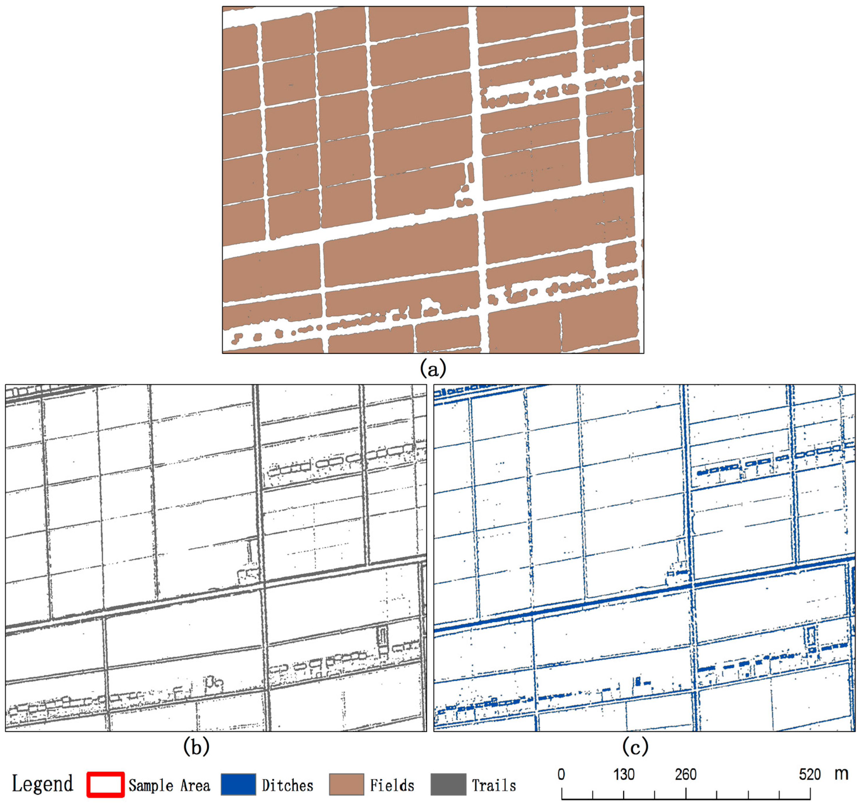
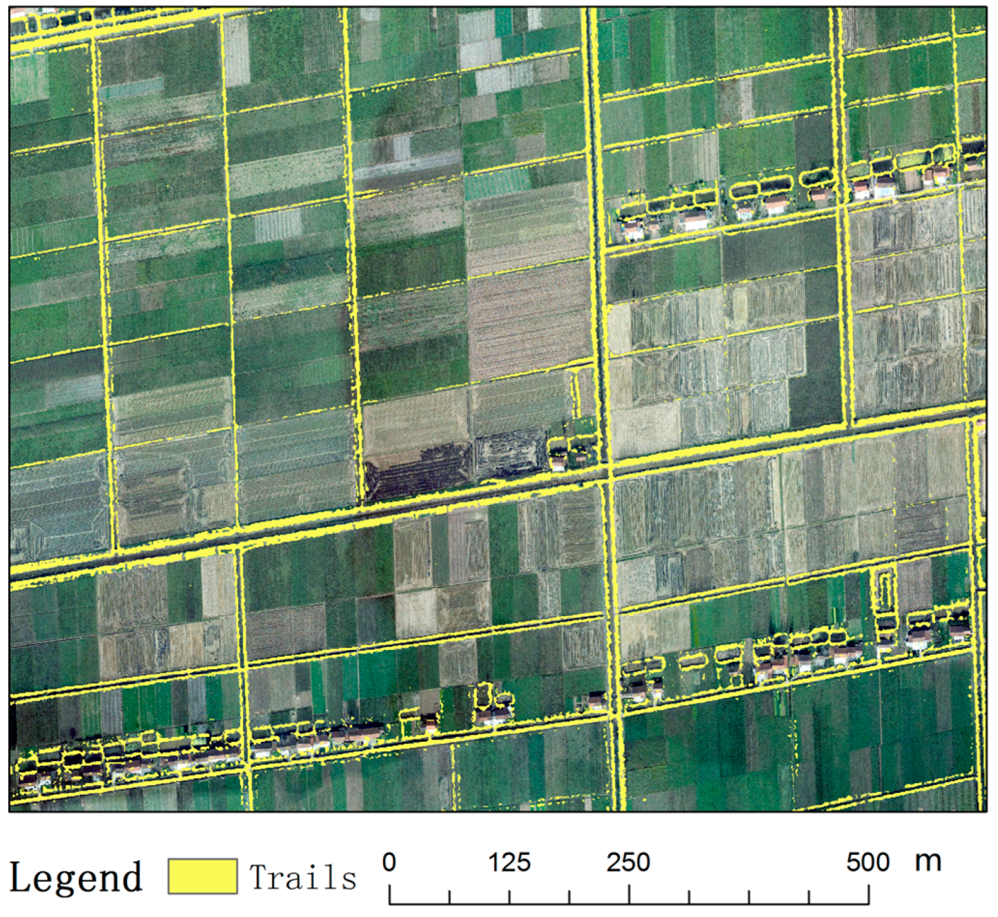
To correct and clarify the results, the polygons converted from the raster results above were generalized to remove peaks, pits, and other small spots. The raster results were converted using the Raster to Polygon tool. Figure 11 shows the trail, ditch, and field polygons for the entire research area, and detailed results are displayed in Figure 12. Over the entire research area, 11,253 cultivated field parcels were extracted, with a total area of 168.7 km2. According to official statistics, Gongshuangcha has 157.6 km2 of farmland; therefore, compared to official statistics, our results of field parcels had an accuracy of 93.42%. Figure 13, for which trail polygons in the sample area were overlaid with an image, shows that the trails agreed with the true ground features. The boundaries of the land parcels were much smoother than those extracted in the previous raster process. The three target features were clearly detected, even those close together were easily discernible, and the method worked well even for those of a relatively small size (Figure 12).
Figure 12 shows that cultivated field parcels, small trails, and ditches crossing farmland could be extracted precisely by this method. In the research area, the smallest trails were about 1 m wide (equivalent to one pixel of the DEM). The smallest size of objects that can be detected depends on the neighborhood size used in the smoothing process and on the data resolution. This approach has the capability of extracting a one-pixel object, which in the context of farmland surveying means that almost all non-cultivable land can be considered. However, a high precision also brings greater errors. Some small errors in the DEM or spots on the ground surface could be enlarged when misrecognized as target objects, which is why there was a small dispersion along the boundaries of some polygons of the target objects.
To assess the efficacy of this method in extracting the three different farmland features, similarity matrices were introduced. Twenty reference areas (each a 20 m radius circle) were chosen at random in the research area. Reference sources were obtained via a visual interpretation of an aerial image of the research area. The image was collected with the LiDAR point cloud with a resolution of 0.2 m. Because trails, ditches, and fields were extracted separately from the same dataset, 3 similarity matrixes are shown using the same 20 reference areas (Table 3, Table 4 and Table 5). In the similarity matrices, rows represent the extracted results and columns represent the reference sources.
The kappa coefficients of over 0.8 indicated a high coherence between the results and the reference sources, and those of between 0.6 and 0.8 indicated substantial coherence. Thus, the results achieved in the Gongshuangcha research area were satisfactory. According to the accuracy assessments, the kappa coefficients were generally high, particularly for trails and fields. For trail extraction, producer’s and user’s accuracies were nearly 90%, and those of field extraction were over 97%. For ditch extraction, the kappa coefficient fell below 0.8 owing to a lack of user’s accuracy.
For the extraction of cultivated fields, other flat blocky objects similar to field parcels (e.g., buildings) were filtered when obtaining the DEM. Only fragmentary small parcels remained and most were smoothed or eliminated; however, some large parcels were still extracted as field parcels. For the extraction of trails, some tiny trails were detected first but eliminated later; the boundaries of some small ponds were extracted as trails.
The ditch extraction user’s accuracy was much lower than the producer’s accuracy. Along some large trails (or levees), bottom lines were often misrecognized as ditches. Bottom lines are the concave parts of levees but are not ditches for irrigation. They are lower than their “levee sides” but are at almost the same elevation as their “field sides”. Additionally, some small ponds were also misrecognized as ditches.
As discussed above, two parameters were important in this approach: the neighborhood size of the smoothing surface and the buffer distance of the generalized polygons. A unique value was chosen for each parameter in the given research area. The values chosen were based on the overall condition (i.e., size of target objects) of the research area and on the need to retain an acceptable balance between efficiency and integrity. However, to achieve efficiency in detecting most of the target objects, some small-scale objects were “sacrificed” (either being smoothed or eliminated), and some large-scale objects were too large to be detected as ribbon-like objects. In future research, to address a greater number of objects at different scales within one research area, an adjustable parameter could be applied on various landforms. Additionally, to avoid the misrecognition of similar objects (such as bushes on slopes), high-resolution images could be overlain on DEMs to obtain more detailed information.
5. Conclusions
Obtaining disaster-forming and -affected information for farmland is the foundation of farmland flood process simulations, flood risk evaluation, and flood-loss evaluation. Particularly in flood plains, flood research requires a high precision. With modern data sources, more precise, efficient, and cheaper surveying methods are required to build efficient farmland flood research methods.
This paper proposes an approach to extract non-cultivable trails, ditches, and cultivated field parcels within farmland on the basis of a high-resolution DEM. The surface was first smoothed and then compared with the original surface. According to this comparison, a primary raster result of the convex, concave, and flat parts of the surface was generated. The raster was then converted into polygons, which were generalized by creating inner and outer buffers.
In experiments on a flood storage and detention area, this method was proven to be effective in extracting farmland features. Particularly for field parcel extraction, the accuracy achieved 93.42%, when compared with official statistics, and the kappa coefficient was 0.90, when compared with a visual interpretation of an aerial image. Most trails and ditches, even those close together, were easily distinguished from cultivated field parcels. However, some small ponds and bottom lines of large levees were misrecognized as ditches. The extraction precision reached one pixel, which meant almost all target objects could be detected.
Many of the farmland features were too small to have reliable differences in some characteristics used to extract similar features in previous research. This approach extracts farmland features according to their physical and spatial characteristics. Compared to existing methods, it does not depend on terrain or vegetation covered, and it performs well on artificial and flat farmland surfaces. LiDAR-derived high-resolution DEM provides a detailed elevation of the ground, which is used as the data source for detecting fine objects.
The polygons extracted covered the position, shape, and area of each non-cultivable trail, ditch, and cultivated field parcel; this method will significantly improve the precision of farmland surveying compared with traditional methods and can offer high-quality data for flood plain farmland flood-process simulations, flood risk evaluation, and flood-loss evaluation.
Acknowledgments
This work was supported by the National Natural Science Foundation of China (Grant No. 41501558) and the National Key Research and Development Program of China (Grant No. 2016YFC0401502).
Author Contributions
Tianlu Qian, Dingtao Shen and Changbai Xi conducted the primary experiments and cartography and analyzed the results. Dingtao Shen and Jie Chen offered data support for this work. Jiechen Wang provided the original idea for this paper.
Conflicts of Interest
The authors declare no conflict of interest.
References
- Woodrow, K.; Lindsay, J.B.; Berg, A.A. Evaluating dem conditioning techniques, elevation source data, and grid resolution for field-scale hydrological parameter extraction. J. Hydrol. 2016, 540, 1022–1029. [Google Scholar] [CrossRef]
- Dottori, F.; Baldassarre, G.D.; Todini, E. Detailed data is welcome, but with a pinch of salt: Accuracy, precision, and uncertainty in flood inundation modeling. Water Resour. Res. 2013, 49, 6079–6085. [Google Scholar] [CrossRef]
- Tan, L.; Liu, J.; Ma, Y.; Liu, H.; Liu, H.; Laurenson, M. Estimation of mountainous farmland area in China based on GIS and RS: A case study of lincheng county. J. Food Agric. Environ. 2009, 7, 769–772. [Google Scholar]
- Yuan, F.; Sawaya, K.E.; Loeffelholz, B.C.; Bauer, M.E. Land cover classification and change analysis of the twin cities (minnesota) metropolitan area by multitemporal landsat remote sensing. Remote Sens. Environ. 2014, 98, 317–328. [Google Scholar] [CrossRef]
- Beuchle, R.; Grecchi, R.C.; Shimabukuro, Y.E.; Seliger, R.; Eva, H.D.; Sano, E.; Achard, F. Land cover changes in the brazilian cerrado and caatinga biomes from 1990 to 2010 based on a systematic remote sensing sampling approach. Appl. Geogr. 2015, 58, 116–127. [Google Scholar] [CrossRef]
- Gutman, G.; Huang, C.; Chander, G.; Noojipady, P.; Masek, J.G. Assessment of the nasa–usgs global land survey (gls) datasets. Remote Sens. Environ. 2013, 134, 249–265. [Google Scholar] [CrossRef]
- Hay, G.J.; Blaschke, T.; Marceau, D.J.; Bouchard, A. A comparison of three image-object methods for the multiscale analysis of landscape structure. ISPRS J. Photogramm. Remote Sens. 2003, 57, 327–345. [Google Scholar] [CrossRef]
- Wu, T.; Luo, J.; Xia, L.; Shen, Z.; Hu, X. Prior knowledge-based automatic object-oriented hierarchical classification for updating detailed land cover maps. J. Indian Soc. Remote Sens. 2015, 43, 1–17. [Google Scholar] [CrossRef]
- Gallay, M.; Lloyd, C.D.; Mckinley, J.; Barry, L. Assessing modern ground survey methods and airborne laser scanning for digital terrain modelling: A case study from the lake district, england. Comput. Geosci. 2013, 51, 216–227. [Google Scholar] [CrossRef] [Green Version]
- Eeckhaut, M.V.D.; Poesen, J.; Verstraeten, G.; Vanacker, V.; Nyssen, J.; Moeyersons, J.; Beek, L.P.H.V.; Vandekerckhove, L. Use of lidar-derived images for mapping old landslides under forest. Earth Surf. Process. Landforms 2010, 32, 754–769. [Google Scholar] [CrossRef]
- Migoń, P.; Kasprzak, M.; Traczyk, A. How high-resolution dem based on airborne lidar helped to reinterpret landforms – examples from the sudetes, SW Poland, Example. Landform Anal. 2013, 22, 89–101. [Google Scholar] [CrossRef]
- Hug, C.; Ullrich, A.; Grimm, A. Litemapper-5600–A waveform-digitizing lidar terrain and vegetation mapping system. Int. Arch. Photogramm. Remote Sens. Spat. Inf. Sci. 2004, 36 Pt 8, W2. [Google Scholar]
- Ackers, S.H.; Davis, R.J.; Olsen, K.A.; Dugger, K.M. The evolution of mapping habitat for northern spotted owls (strix occidentalis caurina): A comparison of photo-interpreted, landsat-based, and lidar-based habitat maps. Remote Sens. Environ. 2015, 156, 361–373. [Google Scholar] [CrossRef]
- Kim, A.M.; Olsen, R.C. Detecting trails in lidar point cloud data. Laser Radar Technol. Appl. XVII. 2012, 8379. [Google Scholar] [CrossRef]
- Azizi, Z.; Najafi, A.; Sadeghian, S. Forest road detection using lidar data. J. For. Res. 2014, 25, 975–980. [Google Scholar] [CrossRef]
- Casas, A.; Riaño, D.; Greenberg, J.; Ustin, S. Assessing levee stability with geometric parameters derived from airborne lidar. Remote Sens. Environ. 2012, 117, 281–288. [Google Scholar] [CrossRef]
- Choung, Y. Accuracy assessment of the levee lines generated using lidar data acquired in the Nakdong River basins, South Korea. Remote Sens. Lett. 2014, 5, 853–861. [Google Scholar] [CrossRef]
- Palaseanu-Lovejoy, M.; Thatcher, C.A.; Barras, J.A. Levee crest elevation profiles derived from airborne lidar-based high resolution digital elevation models in south Louisiana. ISPRS J. Photogramm. Remote Sens. 2014, 91, 114–126. [Google Scholar] [CrossRef]
- Koka, S.; Anada, K.; Nakayama, Y.; Sugita, K.; Yaku, T.; Yokoyama, R. A comparison of ridge detection methods for DEM data. In Proceedings of the Software Engineering, Artificial Intelligence, Networking and Parallel & Distributed Computing (SNPD), Kyoto, Japan, 8–10 August 2012; IEEE: Anaheim, CA, USA, 2003; pp. 513–517. [Google Scholar]
- Koka, S.; Anada, K.; Nomaki, K.; Sugita, K.; Tsuchida, K.; Yaku, T. Ridge detection with the steepest ascent method. Procedia Comput. Sci. 2011, 4, 216–221. [Google Scholar] [CrossRef]
- Bolongaro-Crevenna, A.; Torres-Rodríguez, V.; Sorani, V.; Frame, D.; Ortiz, M.A. Geomorphometric analysis for characterizing landforms in morelos state, mexico. Geomorphology 2005, 67, 407–422. [Google Scholar] [CrossRef]
- Zhong, T.; Tang, G.A.; Zhou, Y.; Li, R.Y.; Zhang, W. Method of extracting surface peaks based on reverse DEMs. Bull. Surv. Mapp. 2009, 4, 35–37. [Google Scholar]
- Soille, P. From mathematical morphology to morphological terrain features. In Digital Terrain Modelling; Springer: Berlin/Heidelberg, Germany, 2007; pp. 45–66. [Google Scholar]
- Xiaomeng, S.; Jianyun, Z.; Chesheng, Z.; Jiufu, L. Advances in digital watershed features extracting based on DEM. Prog. Geogr. 2013, 32, 31–40. [Google Scholar]
- Background Information of Dongting lake. Available online: http://www.dongting.net/news/ShowArticle.asp?ArticleID=474 (accessed on 3 November 2017).
- Xiang, W.; Li, W. Spatial-tanporal distribution of flood and water-logging disasters in dongting lake area and control strategies. Chin. J. Ecol. 2001, 20, 48–51. [Google Scholar]
Figure 1.
Research area.

Figure 2.
Digital Elevation Model (DEM) data of the Gongshuangcha research area.
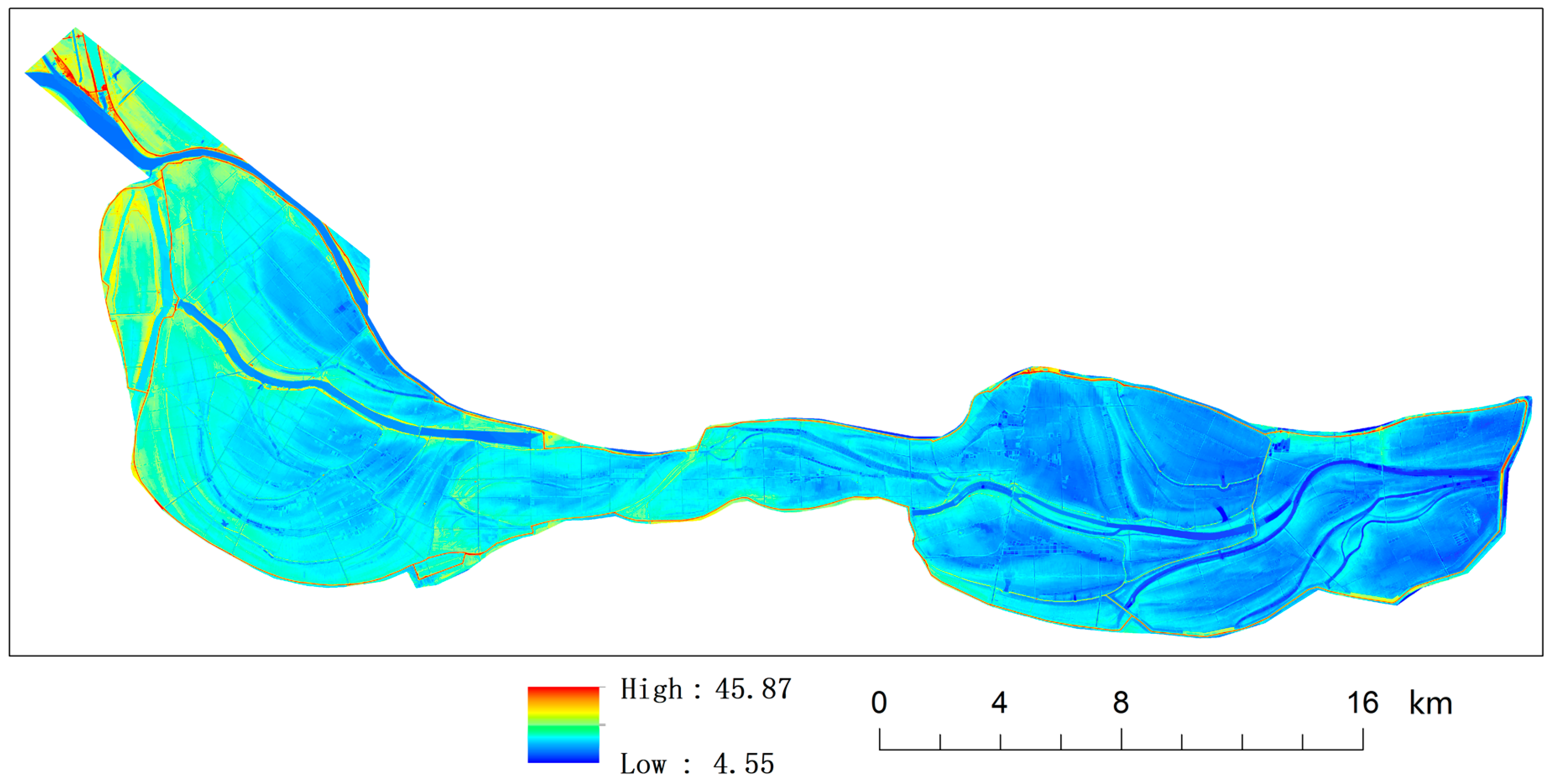
Figure 3.
Ditch, trail, and farmland model.

Figure 4.
Smoothed surface: (a) original surface, and (b) smoothed surface.
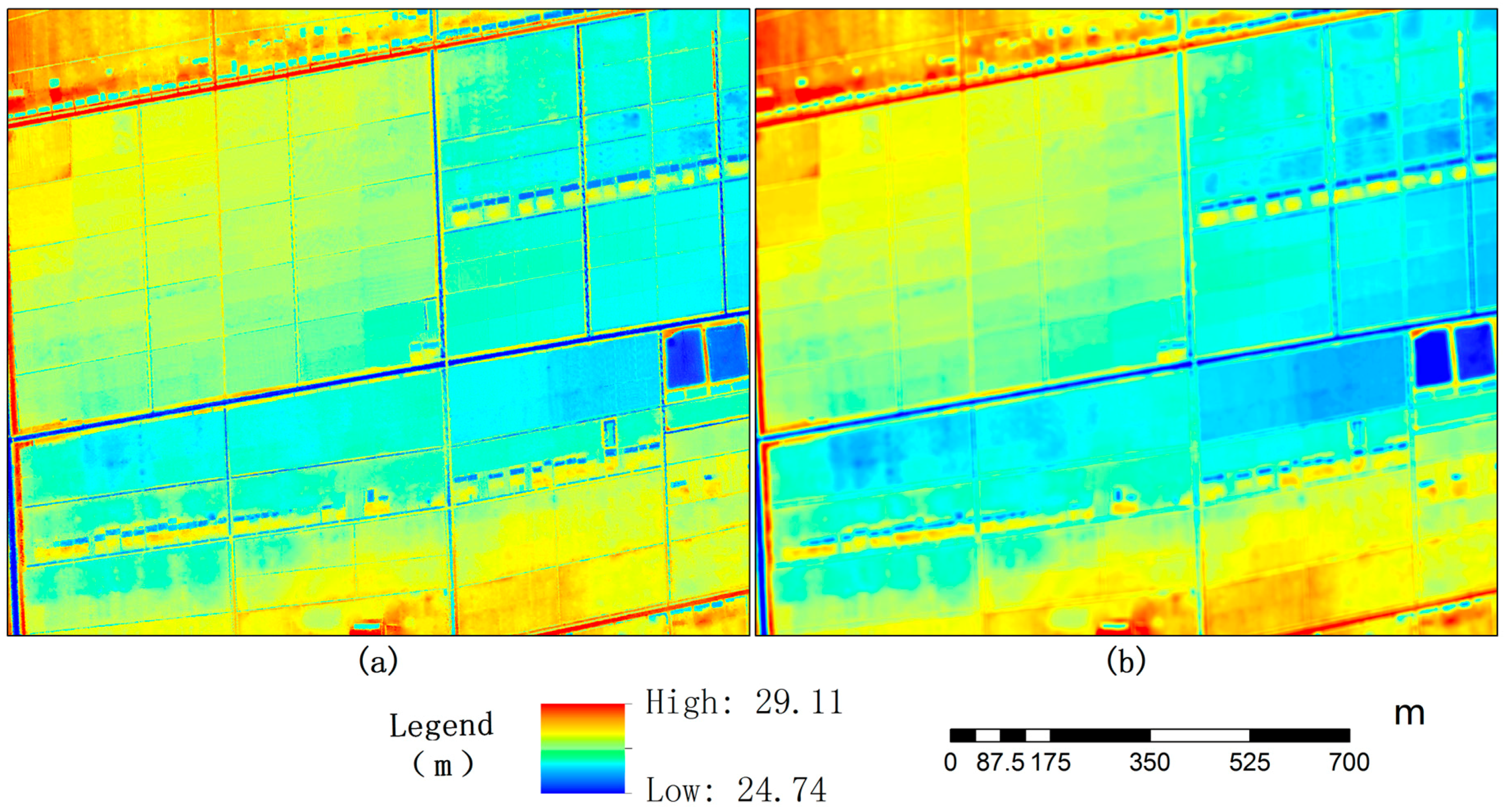
Figure 5.
Defining neighborhood size when smoothing.

Figure 6.
New surface generated by subtraction.

Figure 7.
Filling holes in trail polygons.

Figure 8.
Eroding dispersed spots along trail polygons using different buffer distances: (a) 5 m, and (b) 2 m.
Figure 8.
Eroding dispersed spots along trail polygons using different buffer distances: (a) 5 m, and (b) 2 m.
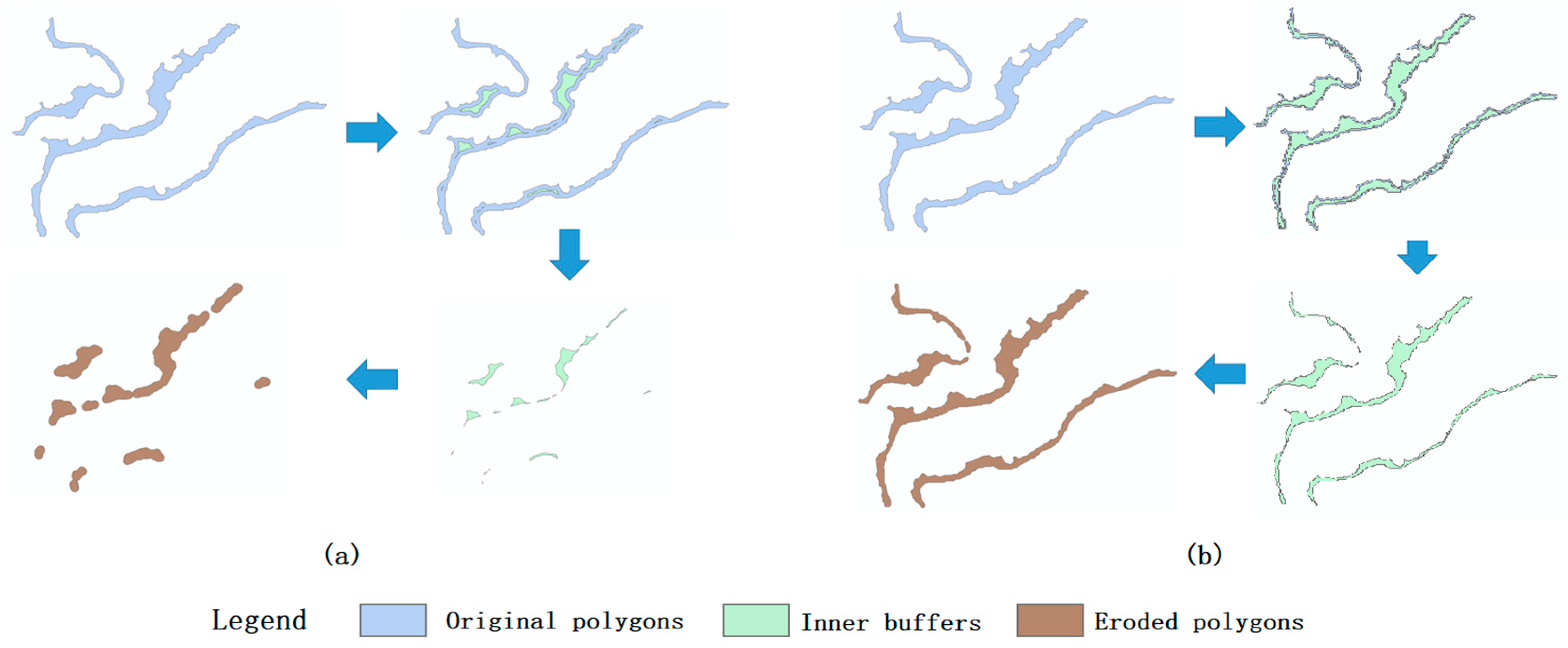
Figure 9.
Raster results of the research area: (a) entire area, and (b) sample area.

Figure 10.
Impact of neighborhood size of the research area: (a) 3 × 3 m neighborhood, and (b) 12 × 12 m neighborhood.
Figure 10.
Impact of neighborhood size of the research area: (a) 3 × 3 m neighborhood, and (b) 12 × 12 m neighborhood.
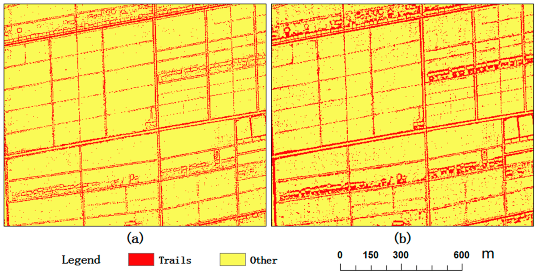
Figure 11.
Vector results of the entire research area: (a) fields, (b) trails, and (c) ditches.
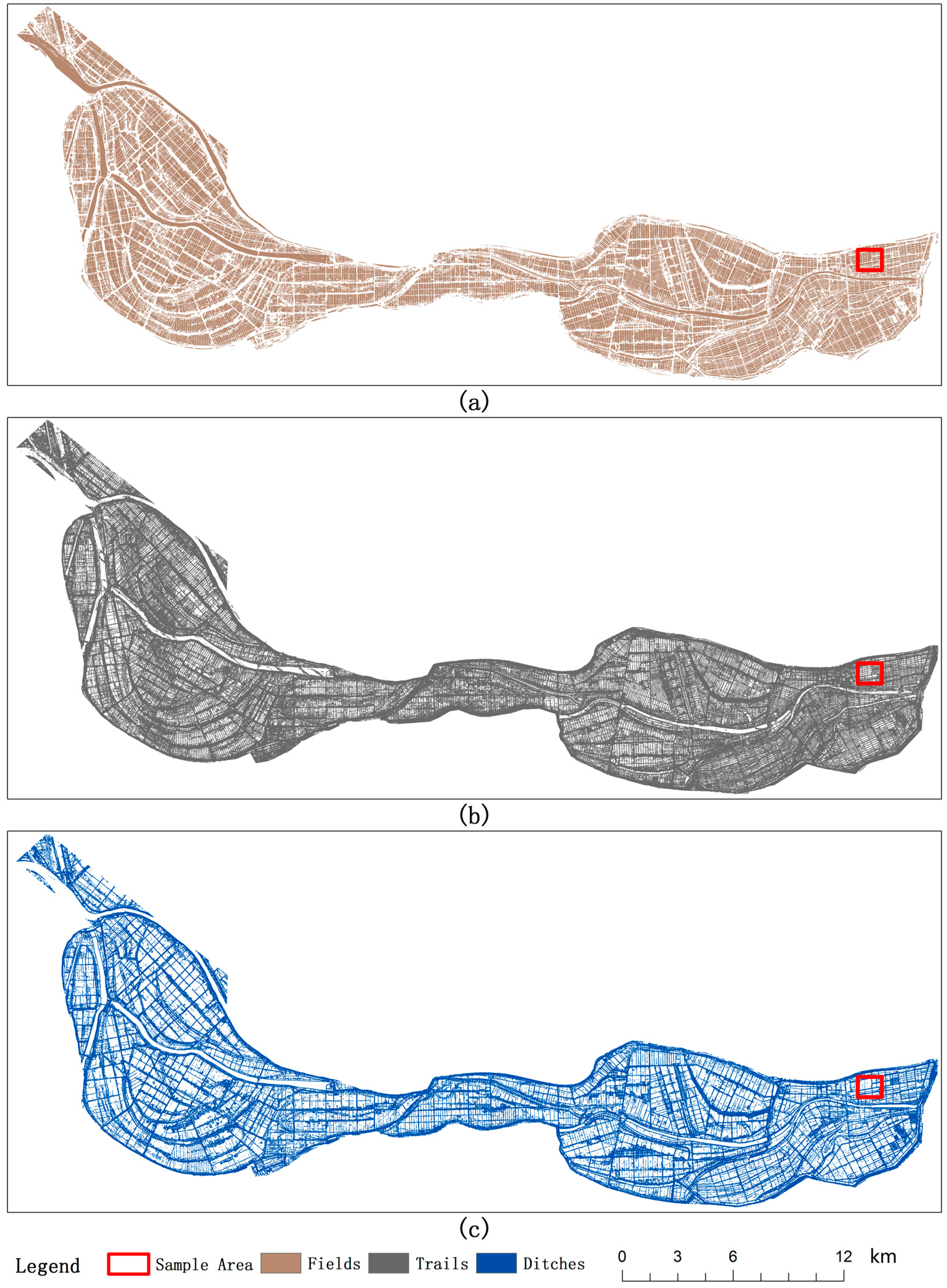
Figure 12.
Detailed vector results of the sample area: (a) fields, (b) trails, and (c) ditches.

Figure 13.
Trail polygons overlaid with an image.


Table 1.
Laser scanner parameters.
| Parameters | Values |
|---|---|
| Model | Riegl LMS-Q680i |
| Field of view | 45°/60° |
| Laser pulse frequency | 80–400 KHz |
| Data acquisition means | Full-band |
| Intensity | 16 bit |
| Scan frequency | 5–160 Hz |
| Laser classification | Class 1 (eye-safe) |
| Position accuracy | x, y < 0.15 m (absolute accuracy) |
| Elevation accuracy | z < 0.25 m (absolute accuracy) |
| Scanning means | Parallel scan |
Table 2.
Camera parameters.
| Model | Rollei Metric AIC Pro (P65+) |
| Focal length | 50 mm |
| Field of view | 56.7° |
| Pixel size | 60 MP |
| Image calibration | Geometry and radiation calibration |
Table 3.
Accuracy assessment of trail results from the research area determined from similarity matrix. Reference sources are 20 visually interpreted reference areas, each a 20 m radius circle.
Table 3.
Accuracy assessment of trail results from the research area determined from similarity matrix. Reference sources are 20 visually interpreted reference areas, each a 20 m radius circle.
| Class Type Determined from Reference Source (m2) | Total (m2) | |||
|---|---|---|---|---|
| Trails | Others | |||
| Class Type Determined From Classified Map (m2) | Trails | 251,514 | 28,658 | 280,172 |
| Others | 33,922 | 2,197,527 | 2,231,449 | |
| Total (m2) | 285,436 | 2,226,185 | 2,511,621 | |
| Producer’s Accuracy | 88.12% | |||
| User’s Accuracy | 89.77% | |||
| Kappa Coefficient | 0.87 | |||
Table 4.
Accuracy assessment of ditch results from the research area determined from similarity matrix. Reference sources are 20 visually interpreted reference areas, each a 20 m radius circle.
Table 4.
Accuracy assessment of ditch results from the research area determined from similarity matrix. Reference sources are 20 visually interpreted reference areas, each a 20 m radius circle.
| Class Type Determined from Reference Source (m2) | Total (m2) | |||
|---|---|---|---|---|
| Ditches | Others | |||
| Class Type Determined From Classified Map (m2) | Ditches | 139,568 | 59,101 | 198,669 |
| Others | 15,116 | 2,297,835 | 2,312,951 | |
| Total (m2) | 154,684 | 2,356,936 | 2,511,620 | |
| Producer’s Accuracy | 90.23% | |||
| User’s Accuracy | 70.25% | |||
| Kappa Coefficient | 0.77 | |||
Table 5.
Accuracy assessment of field results from the research area determined from similarity matrix. Reference sources are 20 visually interpreted reference areas, each a 20 m radius circle.
Table 5.
Accuracy assessment of field results from the research area determined from similarity matrix. Reference sources are 20 visually interpreted reference areas, each a 20 m radius circle.
| Class Type Determined from Reference Source (m2) | Total (m2) | |||
|---|---|---|---|---|
| Fields | Others | |||
| Class Type Determined From Classified Map (m2) | Fields | 1,834,367 | 55,379 | 1,889,746 |
| Others | 39,047 | 582,828 | 621,875 | |
| Total (m2) | 1,873,414 | 638,207 | 2,511,621 | |
| Producer’s Accuracy | 97.92% | |||
| User’s Accuracy | 97.07% | |||
| Kappa Coefficient | 0.90 | |||
© 2018 by the authors. Licensee MDPI, Basel, Switzerland. This article is an open access article distributed under the terms and conditions of the Creative Commons Attribution (CC BY) license (http://creativecommons.org/licenses/by/4.0/).
Share and Cite
MDPI and ACS Style
Qian, T.; Shen, D.; Xi, C.; Chen, J.; Wang, J. Extracting Farmland Features from Lidar-Derived DEM for Improving Flood Plain Delineation. Water 2018, 10, 252. https://doi.org/10.3390/w10030252
AMA Style
Qian T, Shen D, Xi C, Chen J, Wang J. Extracting Farmland Features from Lidar-Derived DEM for Improving Flood Plain Delineation. Water. 2018; 10(3):252. https://doi.org/10.3390/w10030252
Chicago/Turabian StyleQian, Tianlu, Dingtao Shen, Changbai Xi, Jie Chen, and Jiechen Wang. 2018. "Extracting Farmland Features from Lidar-Derived DEM for Improving Flood Plain Delineation" Water 10, no. 3: 252. https://doi.org/10.3390/w10030252
Note that from the first issue of 2016, this journal uses article numbers instead of page numbers. See further details here.