Sensitivity Analysis of the Surface Runoff Coefficient of HiPIMS in Simulating Flood Processes in a Large Basin


1
Key Laboratory of Water Cycle and Related Land Surface Processes, Institute of Geographic Sciences and Natural Resources Research, Chinese Academy of Sciences, 11A, Datun Road, Chaoyang District, Beijing 100101, China
2
College of Urban and Environmental Sciences, Peking University, No.5 Yiheyuan Road, Haidian District, Beijing 100871, China
*
Author to whom correspondence should be addressed.
Water 2018, 10(3), 253; https://doi.org/10.3390/w10030253
Submission received: 5 February 2018
/
Revised: 24 February 2018
/
Accepted: 26 February 2018
/
Published: 1 March 2018
Abstract
:To simulate flood processes at the basin level, the GPU-based High-Performance Integrated Hydrodynamic Modelling System (HiPIMS) is gaining interest as computational capability increases. However, the difficulty of coping with rainfall input to HiPIMS reduces the possibility of acquiring a satisfactory simulation accuracy. The objective of this study is to test the sensitivity of the surface runoff coefficient in the HiPIMS source term in the Misai basin with an area of 797 km2 in south China. To achieve this, the basin was divided into 909,824 grid cells, to each of which a Manning coefficient was assigned based on its land use type interpreted from remote sensing data. A sensitivity analysis was conducted for three typical flood processes under four types of surface runoff coefficients, assumed a priori, upon three error functions. The results demonstrate the crucial role of the surface runoff coefficient in achieving better simulation accuracy and reveal that this coefficient varies with flood scale and is unevenly distributed over the basin.
1. Introduction
Due to rapid urbanization, flood disasters have been globally increasing over the last few decades [1,2,3,4]. The Intergovernmental Panel on Climate Change (IPCC) [5] has stressed that “extreme precipitation events over most of the mid-latitude land masses and over wet tropical regions will very likely become more intense and more frequent by the end of this century, as global mean surface temperature increases”. China has a large area of land in the middle latitudes and has been experiencing unprecedented urbanization for decades. Thus, flood management has been an arduous task for the country.
As a basis of flood management, great progress has been made in developing numerical methodologies (e.g., [6,7,8,9,10,11]). Among them, the two-dimensional hydrodynamic model has become an available technological tool to simulate floods over complex topography (e.g., [12,13,14]).
The development of high-resolution data sources gives the possibility to develop hydrodynamic models at the large basin level. To achieve this, computational acceleration techniques have been greatly progressed in recent years (see, e.g., [15,16,17,18]). Among them, the GPU-based High-Performance Integrated Hydrodynamic Modelling System (HiPIMS) has been favored (see, e.g., [19,20,21,22]) and is the focus of this paper.
The HiPIMS is based on a regular uniform computational grid and fully 2D shallow water equations. In order to deal with rainfall input, an R vector was inserted into HiPIMS as one of the source terms (see in detail [22]). This added term was expressed as the product of a surface runoff coefficient and observed rainfall, instead of solutions based on the Kostiakov equation (e.g., [23]), Green–Ampt model (e.g., [24]), and Richard model (e.g., [25]).
This paper aims to test the sensitivity of the surface runoff coefficient of HiPIMS in terms of different types of floods at the large basin level. The structure of the paper is as follows: Section 2 depicts materials and methods used in the study. The results are presented and discussed in detail in Section 3. Conclusions are given in Section 4.
2. Materials and Methods
2.1. HiPIMS
The fully 2D shallow water equations (Equations (1) and (2)) are employed in HiPIMS based on the Cartesian uniform grids [22].
In Equation (1), q is the vector representing the conserved flow variables; f and g denote the flux vectors in the x- and y-direction, respectively; R, Sb, and Sf are the source terms standing for rainfall, bed slope, and friction, respectively. In Equation (2), h is the water depth (h = η − zb, where η and zb are the water surface elevation and bed elevation above datum, respectively); u and v are the depth-averaged velocity components in the x- and y-direction; g is the acceleration due to gravity; ρ is the water density; r is the rainfall volume (in depth) generating surface runoff during the considered time interval and is obtained by multiplying the surface runoff coefficient (SRC), ranging between [0, 1], and observed rainfall (e.g., [22]); and are the bed slopes in the Cartesian directions; τbx and τby denote the bed friction stresses, which can be calculated by the following formulae.
In Equation (3), the bed roughness coefficient Cf can be calculated by Cf = gn2/h1/3, and n is the Manning coefficient.
In HiPIMS, the above governing equations are solved by a first-order finite volume Godunov-type numerical scheme. The following time-marching formula is used to discretize Equation (1) and update the flow variables:
where the superscript m represents the present time level; Δt is the time step; Ωi is the area of cell i; k is the index of the cell edges (k = [1, 4]); lk stands for the length of the corresponding cell edge; Fk(q) presents the fluxes normal to the cell edges; and n = (nx, ny) defines the unit vector of the outward normal direction. The flux terms and bed slope term are evaluated by an explicit scheme. The friction term is solved by an implicit scheme (see [26]) to maintain the numerical stability when dealing with the surface runoff with small water depth. The surface reconstruction method proposed by [27] is adopted to define the local Riemann problems at the cell interfaces. The Harten-Lax-van Leer-Contact approximate Riemann solver is employed to evaluate the interface fluxes (see [28]). The time step is controlled by the Courant–Friedrichs–Lewy (CFL) criterion. The OpenCL programming framework is implemented to develop a CPU-/GPU-integrating model for high-performance heterogeneous computing. Multiple GPUs can be directly achieved by adopting a domain decomposition technique for medium-/large-scale application (e.g., [20,22]).
2.2. Error Functions
In this study, the simulated discharge is assessed by evaluating the Absolute Relative Error of flood-peak Discharge (ARED) (Equation (5)), the Difference of Peak Arrival Time (DPAT) (Equation (6)), and the Nash–Sutcliffe Efficiency coefficient (NSE) (Equation (7)):
where MAX(Qs) is the maximum simulated discharge, MAX(Qm) is the maximum measured discharge, and ARED ∈ (−∞, +∞);
where TMAX(Qs) is the arrival time of maximum simulated discharge and TMAX(Qm) is the arrival time of maximum measured discharge;
where Qm is the measured discharge, Qs is the simulated discharge, and is the averaged measured discharge.
2.3. Study Area
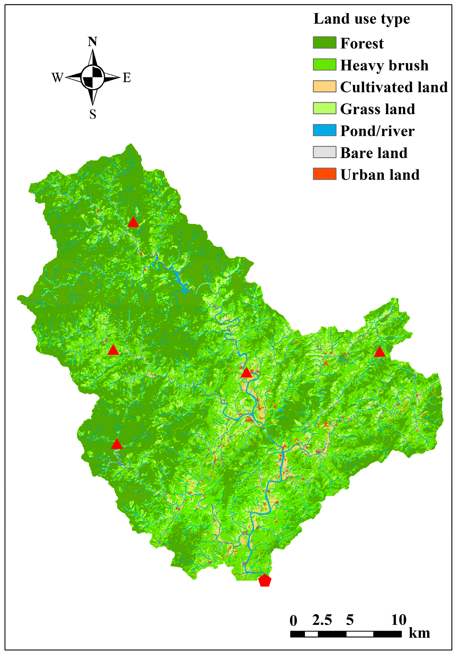
The Misai basin has an area of 797 km2 and is located in south China. The 30 m ASTER GDEM V2 elevation data is used in this study (Figure 1). As shown, mountains in the northwest part of the basin rise to 1242 m and drop steeply towards the plain in the southwest. The elevation of the whole basin ranges from 128 m to 1242 m. There are six precipitation gauging stations and one of them at the outlet of the basin also serves as a stream gauging station (shown in Figure 1). The annual rainfall ranges between 1500 and 2000 mm. Based on 30 m Landsat TM image data and in consideration of the impact of land characteristics on water cycle, the land use type is classified into seven categories—forest, heavy brush, cultivated land, grassland, pond/river, bare land, and urban land (Figure 2). The area proportion and roughness coefficients (Manning’s n) of different land use types are presented in Table 1.
2.4. Typical Flood Processes and Surface Runoff Coefficients
- (1)
- Three different types of flood processes (FPs) were chosen to represent big, medium, and small floods, respectively, as shown in Table 2.
- (2)
- Four types of surface runoff coefficient (SRC) were assumed a priori as below: SRC1 = 0.55, for all grid cells; SRC2 = 0.65, for all grid cells; SRC3 = 0.75, for all grid cells; SRC4: each grid cell was given a SRC based on its land use type—1.0 for urban/pond/river, 0.85 for bared land, 0.7 for farmland/grassland, and 0.5 for forest/heavy brush, as shown in Figure 3.
- (3)
- As such, the above-mentioned FP1, FP2, FP3 and SRC1, SRC2, SRC3, SRC4 then formed twelve combinations and were used for the sensitivity analysis in the following sections. The combination is denoted FPi-SRCj hereafter, e.g., FP1-SRC1 representing FP1 under SRC1.
2.5. Modelling Set
The considered basin was divided into 909,824 grid cells upon a regular uniform grid of resolution 30 m and the rainfall input was given at 1 h intervals based on the historic records from the six gauging stations over the basin. The rainfall distribution was calculated by an inverse distance weighted grid interpolation algorithm with the observed data. The accumulated rainfalls corresponding to the three FPs are shown in Figure 4. The Manning’s n is given in Table 1. The employed hardware included a GTX980ti GPU and an Intel Core I7 4790K CPU desktop. The CFL number is set to be 0.35 in the present work.
3. Results and Discussion
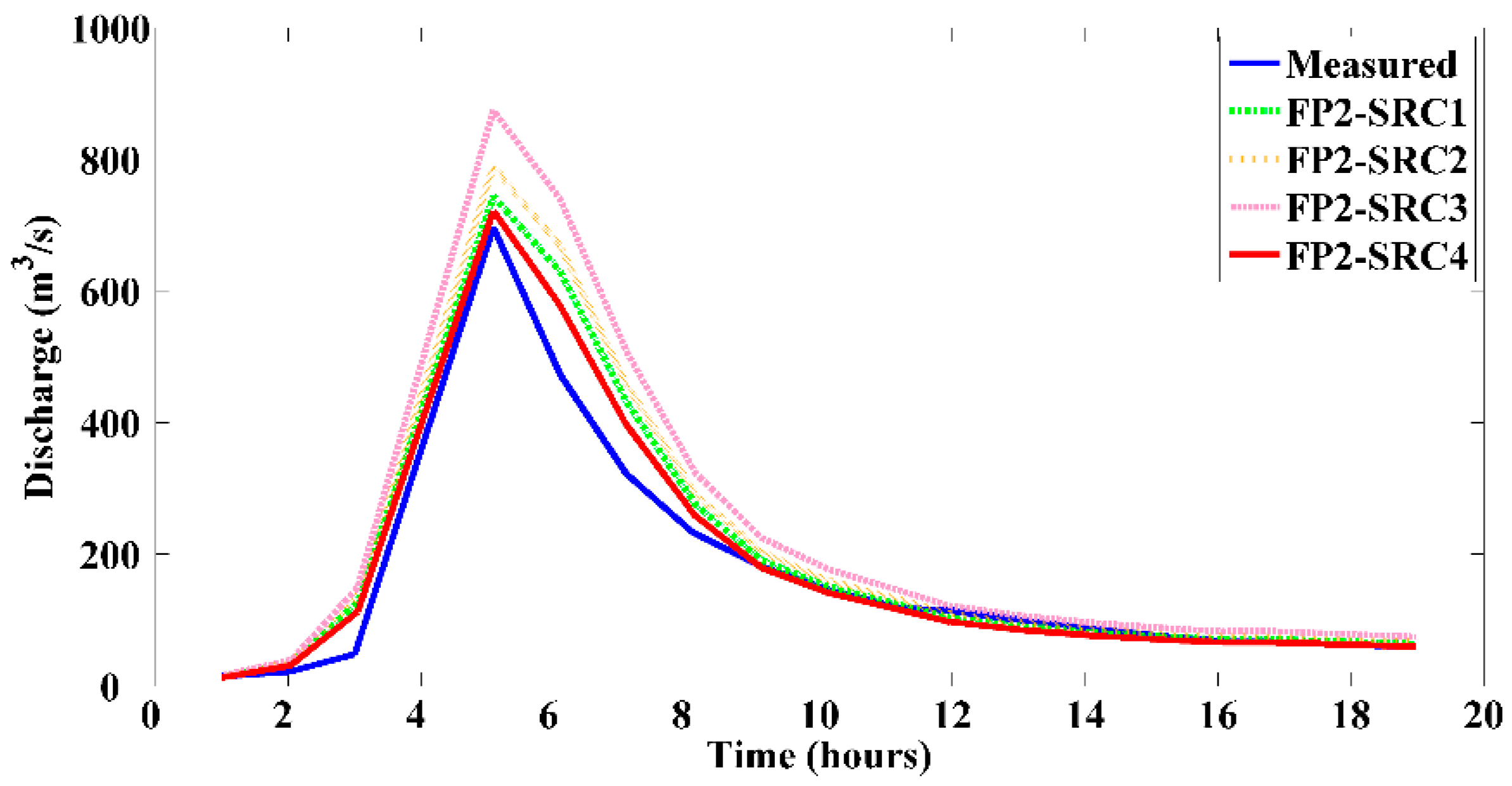
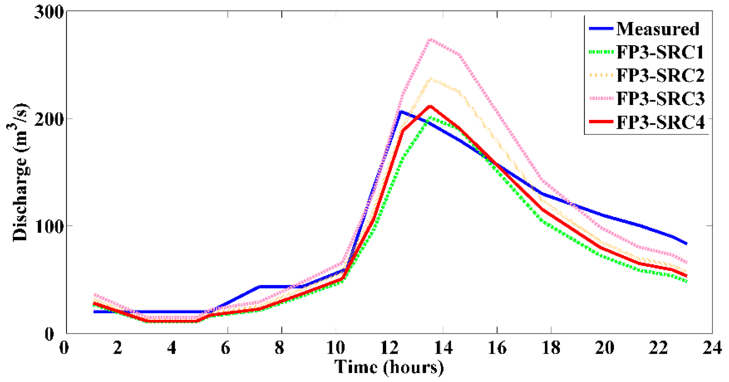
In the present work, the simulations of the twelve combinations using HiPIMS were assessed by comparing the calculated and recorded discharge time series at the outlet gauging station. As shown in Figure 5, Figure 6 and Figure 7, the simulations of the three FPs presented an acceptable agreement with the measurements. However, obvious discrepancies were found among the various combinations.
Further study has been explored through statistical analysis on ARED, DPAT, and NSE. As shown in Table 3, FP1-SRC2, FP2-SRC4, and FP3-SRC1 gave better flood peak simulation in terms of ARED; The simulated arrival time of the flood peak occurred before/after the measured one by no more than 1 h and showed no difference under different SRCs according to DPAT; FP1-SRC4, FP2-SRC4, and FP3-SRC4 obtained better simulated flood processes in the light of NSE. The above results show the potential of HiPIMS in providing satisfactory flood process simulation at the large basin level. Furthermore, it is found that (1) NSE under the four SRCs varies between 0.90 and 0.95 with an average of 0.92 for FP1, between 0.70 and 0.94 with an average of 0.85 for FP2, and between 0.76 and 0.88 with an average of 0.83 for FP3, meaning that the bigger is the FP, the better is the average NSE; (2) the best ARED appears with FP3-SRC1; (3) if only considering SRC1, SRC2, and SRC3, all of which are evenly distributed over the basin, the best NSE comes from FP1-SRC4; And (4) if considering all SRCs, among which SRC4 is uneven over the basin, the best NSE appears in FP1-SRC4. These findings imply that (1) SRC can greatly affect the HiPIMS simulation accuracy and is more sensitive for medium and small floods; (2) SRC varies with flood scale; and (3) SRC is uneven over the basin and is a function of land use type.
4. Conclusions
The sensitivity of the surface runoff coefficient in the HiPIMS source term was tested in the Misai basin with an area of 797 km2 in south China. To this end, the basin was divided into 909,824 grid cells, for each of which its land use type was interpreted from remote sensing data. Considering the twelve combinations composed of three typical flood processes representing big, medium, and small floods, respectively, and four types of surface runoff coefficient assumed a priori, the analysis was conducted upon the three error functions, i.e., the Absolute Relative Error of flood-peak Discharge, the Difference of Peak Arrival Time, and the Nash–Sutcliffe Efficiency coefficient.
The results from the presented work are as follows: (1) demonstrated that HiPIMS has the potential to provide acceptable flood simulation at the large basin level; (2) revealed that the surface runoff coefficient constitutes a remarkable limit in using HiPIMS, and this is especially true for medium and small floods; (3) indicated that this coefficient varies with flood scale and is uneven over the basin; (4) highlighted the need to develop a proper methodology to deal with this source term. In this study, the simulation can be improved by integrating land use information into the application of HiPIMS.
Acknowledgments
The financial support provided by the National Natural Science Foundation of China (Grant No. 51609231 and Grant No. 40471017) is greatly appreciated. The authors would like to acknowledge Liang Qiuhua of the Newcastle University of UK for his kindly providing the HiPIMS software used in this research and especially Xu Chaowei of Peking University for interpreting the land use data.
Author Contributions
Yueling Wang and Xiaoliu Yang conceived and designed the framework of this study, analyzed and discussed the results, and wrote the paper; Yueling Wang treated hydrological data, performed the HiPIMS simulation and conducted statistical analysis.
Conflicts of Interest
The authors declare no conflict of interest. The founding sponsors had no role in the design of the study; in the collection, analyses, or interpretation of data; in the writing of the manuscript, and in the decision to publish the results.
References
- Kundzewicz, Z.W.; Kanae, S.; Seneviratne, S.I.; Handmer, J.; Nicholls, N.; Peduzzi, P.; Mechler, R.; Bouwer, L.M.; Arnell, N.; Mach, K.; et al. Flood risk and climate change: Global and regional perspectives. Hydrol. Sci. J. 2014, 59, 1–28. [Google Scholar] [CrossRef]
- Hirabayashi, Y.; Mahendran, R.; Koirala, S.; Konoshima, L.; Yamazaki, D.; Watanabe, S.; Kim, H.; Kanae, S. Global flood risk under climate change. Nat. Clim. Chang. 2013, 3, 816–821. [Google Scholar] [CrossRef]
- Wang, Y.; Yang, X. Assessing the effect of land use/cover change on flood in Beijing, China. Front. Environ. Sci. Eng. 2013, 7, 769–776. [Google Scholar] [CrossRef]
- Yang, X.; Chen, H.; Wang, Y.; Xu, C. Evaluation of the effect of land use/cover change on flood characteristics using an integrated approach coupling land and flood analysis. Hydrol. Res. 2016, 47, 1161–1171. [Google Scholar] [CrossRef]
- Intergovernmental Panel on Climate Change (IPCC). Summary for Policymakers. In Climate Change 2013: The Physical Science Basis. Contribution of Working Group I to the Fifth Assessment Report of the Intergovernmental Panel on Climate Change; Stocker, T.F., Qin, D., Plattner, G.K., Tignor, M., Allen, S.K., Boschung, J., Nauels, A., Xia, Y., Bex, V., Midgley, P.M., Eds.; Cambridge University Press: Cambridge, UK, 2013; p. 23. [Google Scholar]
- Borga, M.; Anagnostou, E.N.; Blöschl, G.; Creutin, J.-D. Flash flood forecasting, warning and risk management: The HYDRATE project. Environ. Sci. Policy 2011, 14, 834–844. [Google Scholar] [CrossRef]
- Liang, Q.; Xia, X.; Hou, J. Efficient urban flood simulation using a GPU-accelerated SPH model. Environ. Earth Sci. 2015, 74, 7285–7294. [Google Scholar] [CrossRef]
- Yang, T.H.; Yang, S.C.; Ho, J.Y.; Lin, G.F.; Hwang, G.D.; Lee, C.S. Flash flood warnings using the ensemble precipitation forecasting technique: A case study on forecasting floods in Taiwan caused by typhoons. J. Hydrol. 2015, 520, 367–378. [Google Scholar] [CrossRef]
- Douinot, A.; Roux, H.; Garambois, P.A.; Larnier, K.; Labat, D.; Dartus, D. Accounting for rainfall systematic spatial variability in flash flood forecasting. J. Hydrol. 2016, 541, 359–370. [Google Scholar] [CrossRef]
- Miao, Q.; Yang, D.; Yang, H.; Li, Z. Establishing a rainfall threshold for flash flood warnings in China’s mountainous areas based on a distributed hydrological model. J. Hydrol. 2016, 541, 371–386. [Google Scholar] [CrossRef]
- Barbetta, S.; Coccia, G.; Moramarco, T.; Brocca, L.; Todini, E. The multi temporal/multi-model approach to predictive uncertainty assessment in real-time flood forecasting. J. Hydrol. 2017, 551, 555–576. [Google Scholar] [CrossRef]
- Wang, Y.; Liang, Q.; Georges, K.; Jim, W.H. A 2D shallow flow model for practical dam-break simulations. J. Hydraul. Res. 2011, 49, 307–316. [Google Scholar] [CrossRef]
- Hou, J.; Simons, F.; Mahgoub, M.; Hinkelmann, R. A robust well-balanced model on unstructured grids for shallow water flows with wetting and drying over complex topography. Comput. Methods Appl. Mech. Eng. 2013, 257, 126–149. [Google Scholar] [CrossRef]
- Roberts, S.; Nielsen, O.; Gray, D.; Sexton, J.; Davies, G. ANUGA User Manual, Release 2.0; Commonwealth of Australia (Geoscience Australia) and the Australian National University: Canberra, Australia, 2015. [CrossRef]
- Singh, V.P.; Aravamuthan, V. Errors of kinematic-wave and diffusion-wave approximations for steady-state overland flows. CATENA 1996, 27, 209–227. [Google Scholar] [CrossRef]
- Bates, P.D.; Horritt, M.S.; Fewtrell, T.J. A simple inertial formulation of the shallow water equations for efficient two-dimensional flood inundation modelling. J. Hydrol. 2010, 387, 33–45. [Google Scholar] [CrossRef]
- Pender, G.; Néelz, S. Benchmarking of 2D Hydraulic Modelling Packages; Science Report, SC080035/SR2; Environment Agency: Bristol, UK, 2010.
- Liang, Q.; Borthwick, A.G.L.; Stelling, G. Simulation of dam- and dyke-break hydrodynamics on dynamically adaptive quadtree grids. Int. J. Numer. Meth. Fluids 2004, 46, 127–162. [Google Scholar] [CrossRef]
- Smith, L.S.; Liang, Q. Towards a generalised GPU/CPU shallow-flow modelling tool. Comput. Fluids 2013, 88, 334–343. [Google Scholar] [CrossRef]
- Smith, L.S.; Liang, Q. A High-Performance Integrated Hydrodynamic Modelling System for urban flood simulations. J. Hydroinform. 2015, 17, 518–533. [Google Scholar] [CrossRef]
- Liang, Q.; Xia, X.; Hou, J. Catchment-scale high-resolution flash flood simulation using the GPU-based technology. Procedia Eng. 2016, 154, 975–981. [Google Scholar] [CrossRef]
- Liang, Q.; Smith, L.; Xia, X. New prospects for computational hydraulics by leveraging high-performance heterogeneous computing techniques. J. Hydrodyn. 2016, 28, 977–985. [Google Scholar] [CrossRef]
- Bellos, V.; Tsakiris, G. A hybrid method for flood simulation in small catchments combining hydrodynamic and hydrological techniques. J. Hydrol. 2016, 540, 331–339. [Google Scholar] [CrossRef]
- Yin, J.; Yu, D.; Yin, Z.; Liu, M.; He, Q. Evaluating the impact and risk of pluvial flash flood on intra-urban road network: A case study in the city center of Shanghai, China. J. Hydrol. 2016, 537, 138–145. [Google Scholar] [CrossRef] [Green Version]
- Mudd, S.M. Investigation of the hydrodynamics of flash floods in ephemeral channels: Scaling analysis and simulation using a shock-capturing flow model incorporating the effects of transmission losses. J. Hydrol. 2006, 324, 65–79. [Google Scholar] [CrossRef]
- Jin, S. Asymptotic preserving (AP) schemes for multiscale kinetic and hyperbolic equations: A review. Lecture Notes for Summer School on ‘‘Methods and Models of Kinetic Theory” (M&MKT), Porto Ercole (Grosseto, Italy), June 2010. Riv. Mat. Univ. Parma 2012, 3, 177–216. [Google Scholar]
- Xia, X.; Liang, Q.; Ming, X.; Hou, J. An efficient and stable hydrodynamic model with novel source term discretisation for overland flow and flood simulations. Water Resour. Res. 2017, 53, 3730–3759. [Google Scholar] [CrossRef]
- Liang, Q.; Borthwick, A.G.L. Adaptive quadtree simulation of shallow flows with wet-dry fronts over complex topography. Comput. Fluids 2009, 38, 221–234. [Google Scholar] [CrossRef]
- Zheng, Z.; He, S.; Wu, F.; Hu, J. Relationship between surface roughness and Manning roughness. J. Mt. Sci. 2004, 22, 236–239. (In Chinese) [Google Scholar] [CrossRef]
- Tang, X. Characteristics of Runoff and Soil Erosion of Typical Forest Types in the Sources of Qiantang River. Master’s Thesis, Zhejiang A&F University, Hangzhou, China, 22 May 2012. (In Chinese). [Google Scholar]
- Huang, J. Evaluation of Anti-Water Erosion Function of Main Forests in the South Hilly and Mountain Region of Jiangsu Province. Ph.D. Thesis, Nanjing Forestry University, Nanjing, China, 16 June 2011. (In Chinese). [Google Scholar]
Figure 1.
Map of Misai basin.
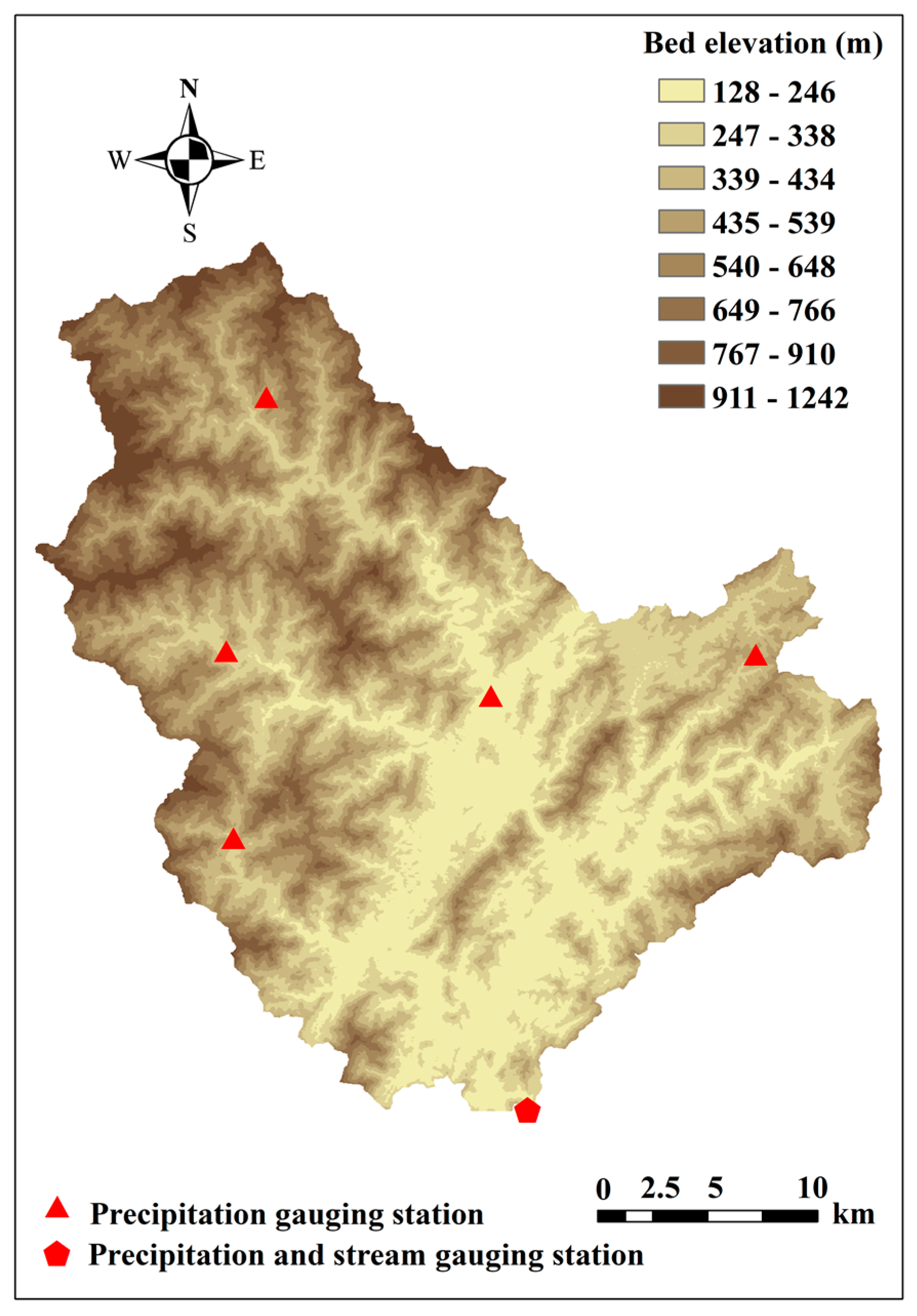
Figure 2.
Land use type of Misai basin.

Figure 3.
The spatial distribution of surface runoff coefficient 4 (SRC4).
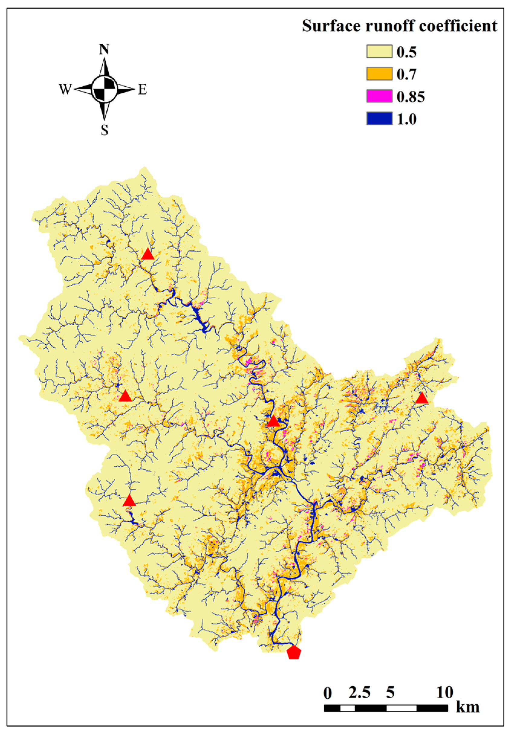
Figure 4.
The spatial distribution of accumulated rainfall of the three flood processes (FPs): (a) FP1; (b) FP2; (c) FP3.
Figure 4.
The spatial distribution of accumulated rainfall of the three flood processes (FPs): (a) FP1; (b) FP2; (c) FP3.
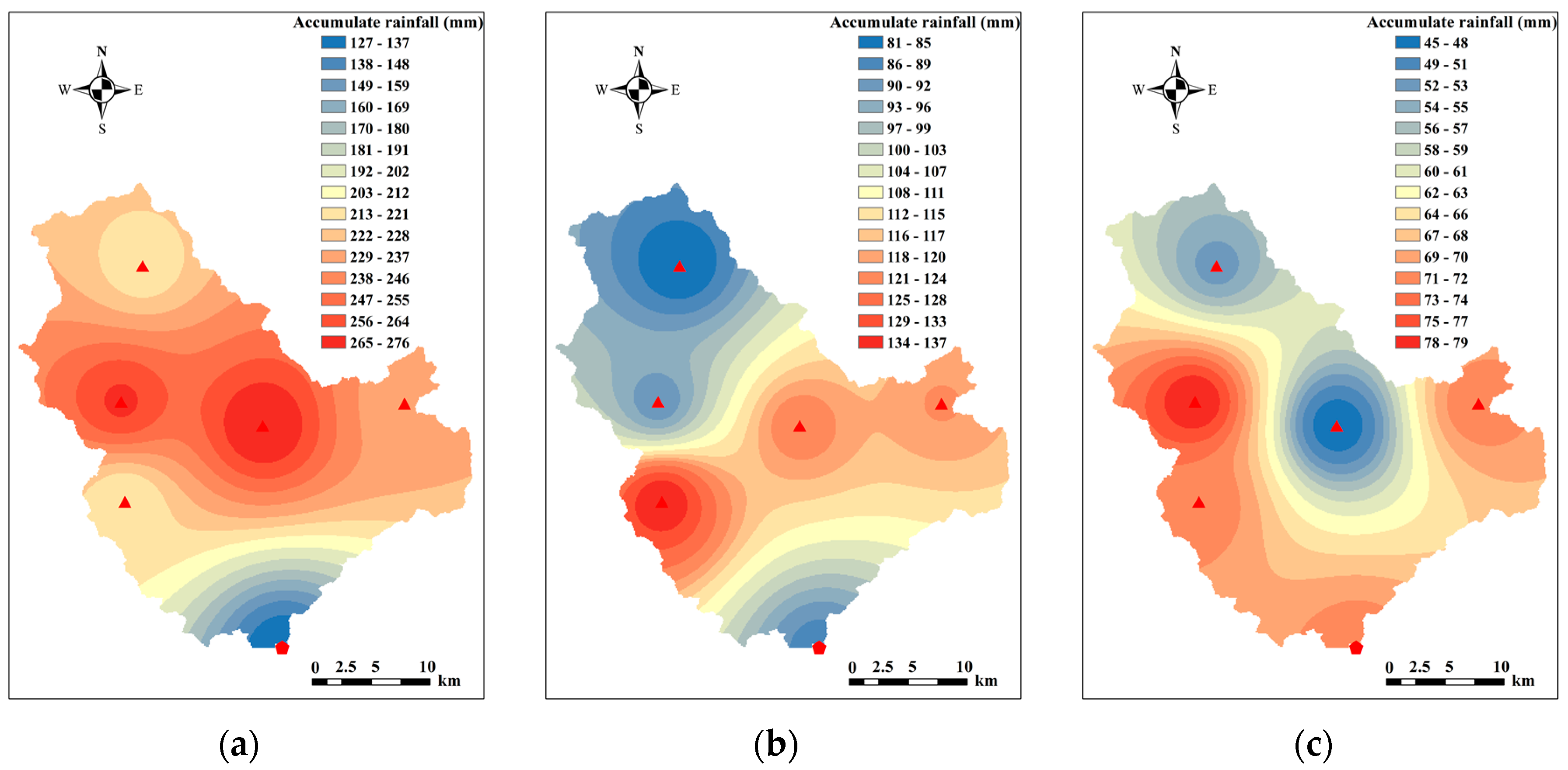
Figure 5.
Comparison of the measured and simulated FP1 under the four SRCs.
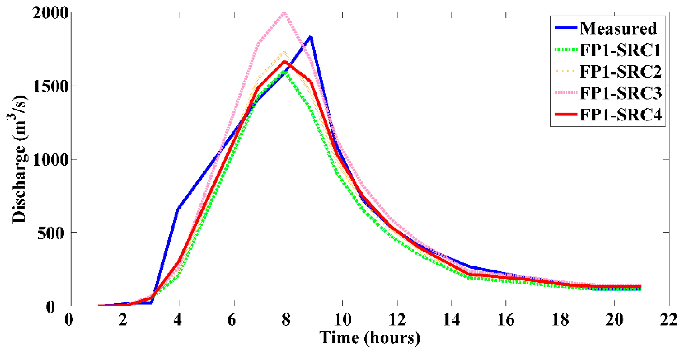
Figure 6.
Comparison of the measured and simulated FP2 under the four SRCs.

Figure 7.
Comparison of the measured and simulated FP3 under the four SRCs.


Table 1.
The area proportion and Manning’s n of different land use types in the Misai basin.
| Land Use Type | Area Proportion (%) | Manning’s n 1 |
|---|---|---|
| Forest | 45.5 | 0.15 |
| Heavy brush | 37.3 | 0.11 |
| Cultivated land | 2.2 | 0.035 |
| Grassland | 7.3 | 0.03 |
| Pond/river | 5.8 | 0.027 |
| Bare land | 0.7 | 0.025 |
| Urban land | 1.2 | 0.016 |
Table 2.
The three typical flood processes.
| Name | Start Time | End Time | Rainfall | Peak Flow |
|---|---|---|---|---|
| FP1 (big) | 29 May 1983, 8:00 | 30 May 1983, 13:00 | 222 mm | 1820 m3/s |
| FP2 (medium) | 5 May 1985, 8:00 | 7 May 1985, 12:00 | 106 mm | 708 m3/s |
| FP3 (small) | 26 May 1987, 8:00 | 27 May 1987, 20:00 | 65 mm | 202 m3/s |
Table 3.
The statistical analysis of the measured and simulated discharge (Q).
| Combination | Measured Q (m3/s) | Simulated Q (m3/s) | ARED (%) | DPAT (h) | NSE |
|---|---|---|---|---|---|
| FP1-SRC1 | 1820 | 1599 | 12.1 | −1 | 0.91 |
| FP1-SRC2 | 1820 | 1732 | 4.8 | −1 | 0.93 |
| FP1-SRC3 | 1820 | 1999 | 9.8 | −1 | 0.90 |
| FP1-SRC4 | 1820 | 1665 | 8.5 | −1 | 0.95 |
| FP2-SRC1 | 708 | 744 | 5.0 | 0 | 0.90 |
| FP2-SRC2 | 708 | 789 | 11.4 | 0 | 0.85 |
| FP2-SRC3 | 708 | 874 | 23.4 | 0 | 0.70 |
| FP2-SRC4 | 708 | 721 | 1.8 | 0 | 0.94 |
| FP3-SRC1 | 202 | 201 | 0.5 | 1 | 0.81 |
| FP3-SRC2 | 202 | 238 | 17.8 | 1 | 0.86 |
| FP3-SRC3 | 202 | 274 | 35.6 | 1 | 0.76 |
| FP3-SRC4 | 202 | 212 | 5.0 | 1 | 0.88 |
© 2018 by the authors. Licensee MDPI, Basel, Switzerland. This article is an open access article distributed under the terms and conditions of the Creative Commons Attribution (CC BY) license (http://creativecommons.org/licenses/by/4.0/).
Share and Cite
MDPI and ACS Style
Wang, Y.; Yang, X. Sensitivity Analysis of the Surface Runoff Coefficient of HiPIMS in Simulating Flood Processes in a Large Basin. Water 2018, 10, 253. https://doi.org/10.3390/w10030253
AMA Style
Wang Y, Yang X. Sensitivity Analysis of the Surface Runoff Coefficient of HiPIMS in Simulating Flood Processes in a Large Basin. Water. 2018; 10(3):253. https://doi.org/10.3390/w10030253
Chicago/Turabian StyleWang, Yueling, and Xiaoliu Yang. 2018. "Sensitivity Analysis of the Surface Runoff Coefficient of HiPIMS in Simulating Flood Processes in a Large Basin" Water 10, no. 3: 253. https://doi.org/10.3390/w10030253
Note that from the first issue of 2016, this journal uses article numbers instead of page numbers. See further details here.