Application of an Automated Discharge Imaging System and LSPIV during Typhoon Events in Taiwan


1
Department of Civil and Disaster Prevention Engineering, National United University, Miaoli 36063, Taiwan
2
College of Engineeing and Science, National United University, Miaoli 36063, Taiwan
3
Department of Marine Environmental Informatics, National Taiwan Ocean University, Keelung 20224, Taiwan
*
Author to whom correspondence should be addressed.
Water 2018, 10(3), 280; https://doi.org/10.3390/w10030280
Submission received: 12 February 2018
/
Revised: 5 March 2018
/
Accepted: 5 March 2018
/
Published: 7 March 2018
Abstract
:An automated discharge imaging system (ADIS), which is a non-intrusive and safe approach, was developed for measuring river flows during flash flood events. ADIS consists of dual cameras to capture complete surface images in the near and far fields. Surface velocities are accurately measured using the Large Scale Particle Image Velocimetry (LSPIV) technique. The stream discharges are then obtained from the depth-averaged velocity (based upon an empirical velocity-index relationship) and cross-section area. The ADIS was deployed at the Yu-Feng gauging station in Shimen Reservoir upper catchment, northern Taiwan. For a rigorous validation, surface velocity measurements were conducted using ADIS/LSPIV and other instruments. In terms of the averaged surface velocity, all of the measured results were in good agreement with small differences, i.e., 0.004 to 0.39 m/s and 0.023 to 0.345 m/s when compared to those from acoustic Doppler current profiler (ADCP) and surface velocity radar (SVR), respectively. The ADIS/LSPIV was further applied to measure surface velocities and discharges during typhoon events (i.e., Chan-Hom, Soudelor, Goni, and Dujuan) in 2015. The measured water level and surface velocity both showed rapid increases due to flash floods. The estimated discharges from ADIS/LSPIV and ADCP were compared, presenting good consistency with correlation coefficient R = 0.996 and normalized root mean square error NRMSE = 7.96%. The results of sensitivity analysis indicate that the components till (τ) and roll (θ) of the camera are most sensitive parameters to affect the surface velocity using ADIS/LSPIV. Overall, the ADIS based upon LSPIV technique effectively measures surface velocities for reliable estimations of river discharges during typhoon events.
1. Introduction
Accurate measurement of stream flows, which plays a critical role in hydrological processes, is highly desirable for many practical applications (like flood management and reservoir operation) especially during typhoon events [1,2]. Typically, some gauging stations are established at upstream rivers to provide essential information for earlier warning. However, the surrounding environments can be dangerous and hardly accessible. Meanwhile, most flow measurements in current operation practice are intrusive and involve complex user-assisted procedures. Thus, flood discharge measurements are still rare and challenging.
To date, both (i) intrusive; and, (ii) non-intrusive approaches have been developed to measure stream flows. Conventionally, river discharge measurement is conducted using current meters, dye concentrations, or acoustic methods (e.g., acoustic Doppler current profiler, ADCP). In combination with recorded water levels, a stage-discharge relationship (known as the rating curve) can be established [3]. Besides, recourse will be made to maintain the reliable rating curve for a natural river (which often presents changing characteristics due to channel encroachment, dredging, weed growth, or other reasons). However, these intrusive approaches would hinder direct measurements under extreme weather, posing the concern of great uncertainties and questionable accuracy in extrapolated high flow rates [4].
In recent years, non-intrusive approaches based on radar (e.g., [5]) and/or imaging systems (e.g., [6,7,8,9,10,11,12,13,14,15,16]) have been increasingly applied, providing a safer alternative for measuring flood discharge. Without the needs of human-operated physical sampling and data acquisition, surface velocities are characterized from continuous images of observed (seeded fluid) flows mainly using two types of algorithms, i.e., particle tracers and imagine analyses (e.g., [17]). In the former method, the particle tracking velocimetry (PTV) returns one vector for each particle, and is therefore more suitable for low seeding cases. In contrast, particle image velocimetry (PIV), which is used in the later one, can track the average motion of a particle group within an image.
The Large Scale Particle Image Velocimetry (LSPIV) originated from the lab-scale techniques is a promising tool for safely monitoring natural flows in different regimes. Recently, LSPIV has been successfully applied in various environmental studies, e.g., estimations of hydrodynamic characteristics in riverine environment [7,18] and flow patterns in limnological ecosystems [19]. The LSPIV also provides a novel hydrometric tool for gauged stations and ungauged sites in watershed. At a gauging station, LSPIV enables discharge measurement over a broader range of flow conditions than those traditional methods. Uncertainties of the extrapolated portion in a rating curve can be alleviated. On the other hand, at an ungauged site (without any hydrological data and rating curve), flow discharges can be obtained with reasonable uncertainties based upon hydraulic assumptions from in-situ characteristics [20].
The objective of this study is to apply an automated discharge imaging system (ADIS) for estimating flash floods in an upper watershed based upon the dual-camera framework and LSPIV technique. With measured surface velocities, stream discharges are calculated from the depth-averaged velocities (using an empirical velocity-index relationship) and cross-section area. The ADIS was deployed at the Yu-Feng gauging station in the Shimen Reservoir catchment of northern Taiwan. Surface velocities and discharges during four typhoon events (i.e., Chan-Hom, Soudelor, Goni, and Dujuan) in 2015 were measured. To validate the newly developed ADIS, several conventional measurements were also conducted using the acoustic Doppler current profiler (ADCP) (Son Tek, San Diego, CA, USA) and surface velocity radar (SVR) (Applied Concepts, Richardson, TX, USA).The sensitivity analysis was conducted by varying interior and exterior parameters at right and left cameras in order to comprehend the important parameters that affect the surface velocity using ADIS/LSPIV.
2. Materials and Methods
2.1. Description of the Study Area
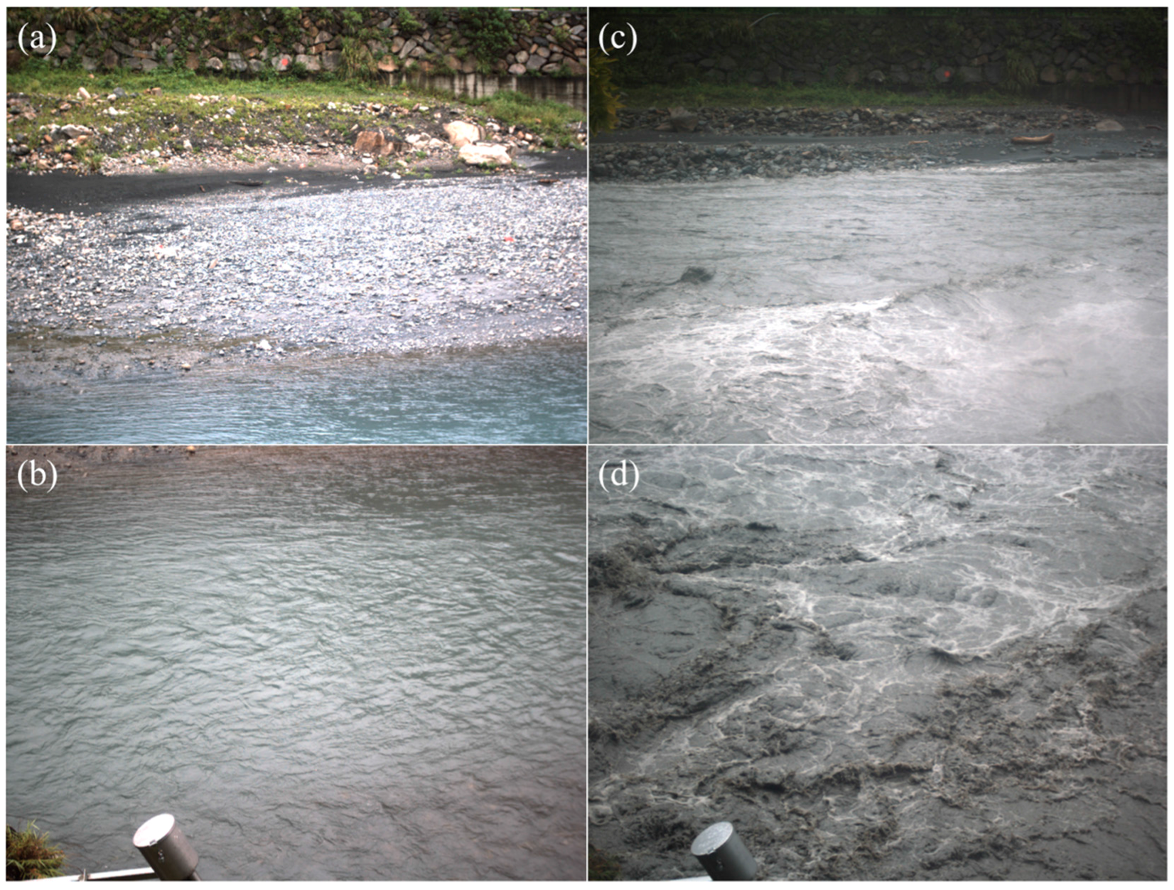
The selected study site is the Yufeng gauging station with an elevation of 684 m, located at the upstream Yufeng Creek, upper catchment of Shimen Reservoir, northern Taiwan (Figure 1). The river bed of Yufeng Creek is occupied with gravel and stone. The cross section (near the study site) has a width of 15~30 m with an average depth of 1.5 m at the normal flow condition. The Yufeng gauging station, which is maintained by the Northern Region Water Resources Office, Water Resources Agency, is equipped with an automated pressure sensor to measure water level. The dual-camera system (see the detailed description below) is installed at the platform of Yufeng gauging station. This platform is about at a height of 10 m above the river bed with a distance of 15~80 m to the observation area. Figure 2 displays some images obtained from the dual-camera system during normal flow condition and Typhoon Soudelor in August 2015. It can be seen that the exposed gravel area was inundated during typhoon event.
2.2. ADIS Hardware System
For hardware setting, two industrial cameras (DMK 23G274 from The Imaging Source) are used in the ADIS. With progressive scanning CCD sensors (The Imaging Source, Taipei, Taiwan), each camera can capture 1.92-megapixel (or 1600 × 1200-pixel) images at a frame rate of 20 FPS. In addition, real-time adjustments for proper light exposure and shutter speed under different conditions are controlled remotely using a server computer from the gauging station. The video image signals are directly transferred back to the Frame Grabbers (on computer) via a GigE cable connection.
A dual-camera system (that consists of near- and far-field cameras) with 15-mm C-mount machine vision lenses was designed (see Figure 3a) to obtain high-resolution images over the entire cross section of Yufeng Creek. The near- and far-field regions are partly overlapped with areas of 12 m × 20 m and 40 m × 50 m (the flow direction × cross-sectional direction), respectively. In the areas of interest, the image resolution is in the range of 4.35 (near-field camera)–23.5 (far-field camera) mm/pixel.
The parameters of dual-camera system should be established and resolved using control points. In total, 44 control points were arranged on the stairs at Yufeng station (see Figure 3c) and measured by the total station (see the locations of control points and cameras in Figure 3d). The dual-camera system would turn horizontally between the control points and river channel (in positive and negative y directions, respectively) during the parameter calibration and flow measurement procedures.
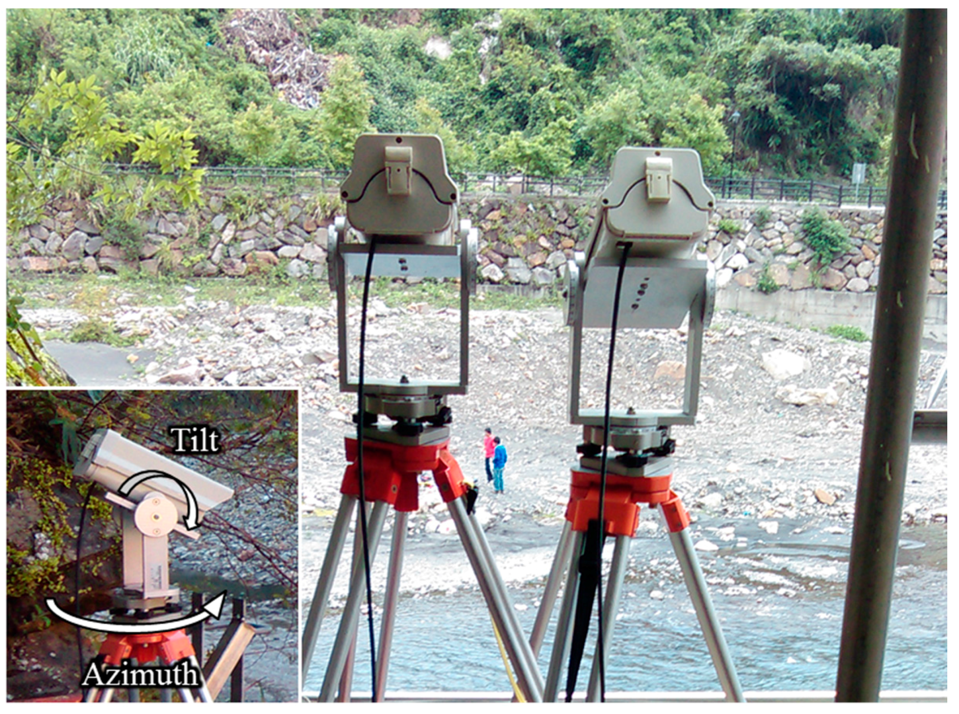
To protect the hardware system, both cameras were enclosed in weatherproof cases, which were also sealed with rubber gaskets to prevent water leaking (Figure 4). The enclosure cases were mounted on custom-made pan-tilt heads which were built on high-quality survey tribrachs. Thus, the cameras can be precisely rotated in the tilt (about vertical axis) and azimuth (about horizontal axis) directions for a desired image view (see the inset part in Figure 4).
2.3. ADIS Software System
The ADIS software system for the automatic measurement of surface velocities and discharges was developed using MATLAB language. This program mainly (i) solves camera parameters for image calibration; (ii) maps images to the physical coordinate system; (iii) measures surface velocities using LSPIV; and, (iv) calculates the discharge of the river by a velocity-index approach. The program of ADIS software which was developed by our team can be used to calibrate cameras in the field and to capture images, which are mapped to the physical coordinate system. The velocity field across the cross section can be extracted and calculated from images. Then, the discharge is obtained according to velocity-index approach and velocity-area method. In the following, detailed LSPIV algorithms are given.
- (i) Image Calibration
A two-step calibration procedure was applied before mapping the raw images to a physical coordinate. First, the so-called interior calibration was used to correct radial and tangential distortions (commonly appeared in the photographs from spherical-lens cameras). The distortion parameters are defined by the collinearity equations can be found in Wanek and Wu [21]. In Figure 5, the parameters, (uc, vc), represent the center of the image; r is the distance from image center to an arbitrary point; (k1, k2) and (p1, p2) are the lens parameters of radial and tangential distortions, respectively.
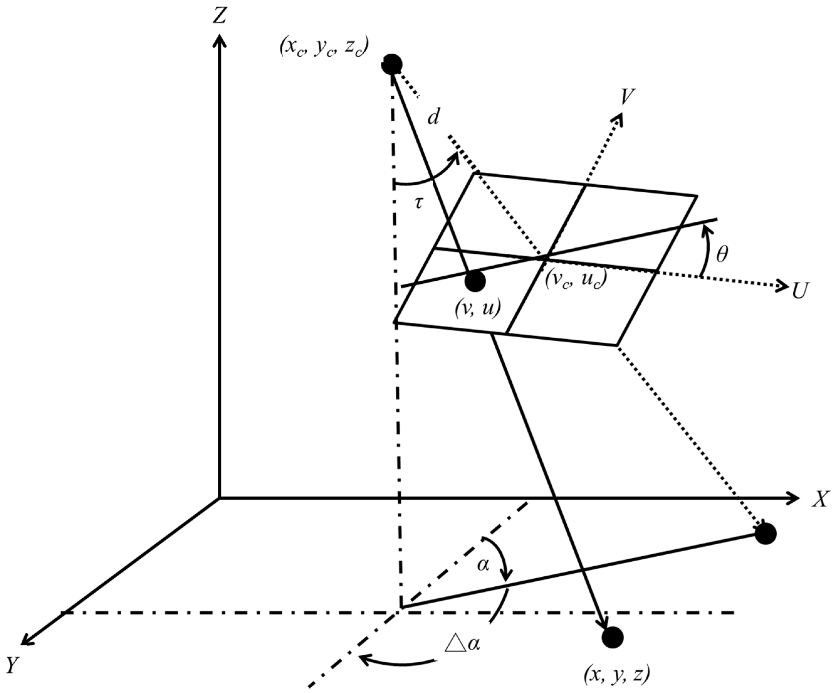
Next, the exterior calibration based upon a pinhole camera model (see Figure 5) was adopted to determine a geometric relationship between an image point (u, v) and its physical position in space (x, y, z). In Figure 5, d is the focal length of camera lens; xc, yc, zc are the physical locations of the cameras; coefficients rij are rotational angles (i.e., components of azimuth α, tilt τ, and roll θ) of the camera [22]. The detailed formulas to express a geometric relationship between an image point (u, v) and physical position in space (x, y, z) can be found in Bechle et al. [13].
The procedure of interior calibration is used to obtain the parameters (uc, vc and d), while the procedure of exterior calibration is used to yield the parameters (xc, yc, zc, α, τ and θ). Based on the procedure of interior and exterior calibrations, the parameters of right and left cameras are obtained and are shown in Table 1.
For robust/accurate image calibration, a large number (at least more than 15) of high-quality control points are essential [22]. In the present study, 44 control points were established and measured using a total station (see the image in Figure 3 for their distribution and physical coordinates). Also, a rotational calibration technique was developed for the in-situ conditions. The basic idea was to rotate both of the cameras between the observation region (river channel) and an area (stairs) where the control points existed. The rotational calibration can be conducted before/after image acquisition since our cameras always can be rotated back to the initial orientation α [13]. The main reason that the control points are selected at stairs in the gauging station is to prevent the researchers who intrude the river channel region for measuring the physical coordinates using total station. The other one reason is that if the control points are set in the river channel region, they should be inundated when river banks are flooded during the typhoon events.
Note that 30 known control points were utilized to determine camera parameters and the rest 14 points were further used to examine the accuracy of image calibration. Based upon the resolved parameters from rotational calibration approach, the images of right and left cameras can adequately estimate the positions of those testing points with average errors of 0.82 and 2.2 cm, respectively.
- (ii) Image Mapping
A quasi three-dimensional approach was adopted to map each recorded image to the physical coordinate system. Two images (at least) were taken from different vantage points to triangulate three-dimensional coordinates of water surface [13,21,23]. Based on the camera orientation parameters, two conditions are insufficient to resolve the three unknowns (x, y, z) for image points (u, v) in either near- or far-field observation area. By the quasi three-dimensional approach in which automatic gauged water level z from the Yufeng gauging station was provided, therefore, the corresponding location (x, y) of a featured object can be determined. The same approach of image mapping that was used by Bechle et al. [13] was employed in current study.
Note that the free surface of shallow-water flow [24] was assumed to be relatively flat and parallel to the XY plane. At current study site (i.e., Yufeng gauging station), measurement results from a level meter indicated that slope of water surface was generally smaller than 0.002 in the flow direction. Along the centerline of Yufeng Creek, changes in water levels were about only ±1.5 cm from the mean. In this study, the use of mean water level merely caused a tiny error of 0.01 cm in estimated horizontal position, supporting validity of flat water surface assumption.
- (iii) Velocity Measurement
Surface velocity, including its magnitude and direction, is a valuable indicator to the discharge condition of a river. In this study, the LSPIV tracking motion of features on water surface over time was used to measure surface velocity. The procedure for LSPIV analysis is described as follows. First, images are selected from those created ortho-photos (in the previous image mapping step) using a constant time interval, e.g., a time step Δt = 0.05 s in this study. Second, two successive images (A and B) are used to analyze the velocity field. Image A is divided into a uniform grid of subarrays, which are known as interrogation areas. The dimension of interrogation areas (100 × 100 pixels) can be decided according to the size of flow patterns [7]. A subarray is then moved and located in Image B with an image intensity correlation method to determine the displacement of interrogation areas. The most likely displacement of the visible features on water surface is determine as the maximum cross-correlation coefficient computed between two ensembles of gray-scale pixels in interrogation areas [20]. The overlap between interrogation areas in two successive images is 50% for typhoon event and 95% for normal flow condition. Such interrogation areas (100 × 100 pixels) were adequate to capture the motion of surface water.
Ten images (i.e., 0.5 s) were used to obtain the time averaged velocity field. The image resolution is not modified for LSPIV analysis. Because the time averaged velocity field was calculated automatically in the field, all images were recorded and saved in the computer. All velocity values across the image are simply averaged. The measured data before averaging is not smoothed and processed, therefore, no range for measured velocity using LSPIV is defined.
In this study, the LSPIV method was further when compared with other instruments for surface velocity measurements, including Stalker Pro II surface velocity radar (SVR) and SonTek acoustic Doppler current profile (ADCP). For the measurement capability of SVR (and ADCP), flow velocities up to 18.0 m/s (and 20.0 m/s) can be well captured (with errors smaller than 1%). The location of ADCP and SVR data acquisition campaign along cross-section is shown in Figure 3a.
- (iv) Discharge Calculation
The river discharge was calculated using a velocity-index approach that relates the surface velocity (Vsurf) obtained from LSPIV to a depth-averaged one (Vdepth-avg), i.e.,
and
where is the measured stream discharge obtained from ADCP; A is the cross-section area; k is the surface correction factor (i.e., velocity index). The depth-averaged velocity (Vdepth-avg) is obtained from ADCP measurement. In the laboratory, a surface correction factor based upon a parabolic vertical velocity profile was determined, i.e., k = 0.95 [25]. In the field, the correction factor k is site-specific and may show significant variability among various hydraulic/hydrologic conditions. Generally, correction factors present an increasing trend with water stages, e.g., k = 0.85 for the baseflow and k = 0.93 at a high flow condition [7].
In this study, a velocity-index relationship for ADIS was established based on the depth-averaged velocity derived from the ADCP cross-sectional measurement results. Once the correction factor is obtained, river discharges can be readily estimated from the surface velocities using Equations (3) and (4). Note that velocity fields from concurrent surveys with a standard velocity-area method [26] were also employed to calculate total river discharge (sum of products of depth-averaged velocity and area in divided subsections) for further comparison (or validation).
3. Results and Discussion
The costs of ADIS and ADCP instruments for measuring velocity are about 8 thousand and 70 thousand United States (US) dollars, respectively. Our ultimate goal is to promote this cost-effective ADIS for practical operations in the near future.
In the present study, the aim is to examine the performance of ADIS. In this section, the measured surface velocities using different instruments (i.e., LSPIV, ADCP, and SVR) were compared during normal flow first, followed by extreme-flow applications during typhoons in 2015. The ADCP and SVR instruments can not be used for flow measurement during typhoons because the surveyors are exposed to danger. Therefore, there is no other measurement that is available for comparison during typhoon events.
The analyzing approach using ADIS for normal flow and for typhoon event is same. The normal flow condition is defined as no rainfall during the measured date (see Table 2). The ADIS measurement for typhoon events in 2015 include Typhoon Chan-Hom (10–12 July), Typhoon Soudelor (7–9 August), Typhoon Goni (23–25 August), and Typhoon Dujuan (28–30 September).
3.1. Comparison of Surface Velocity from Different Instruments
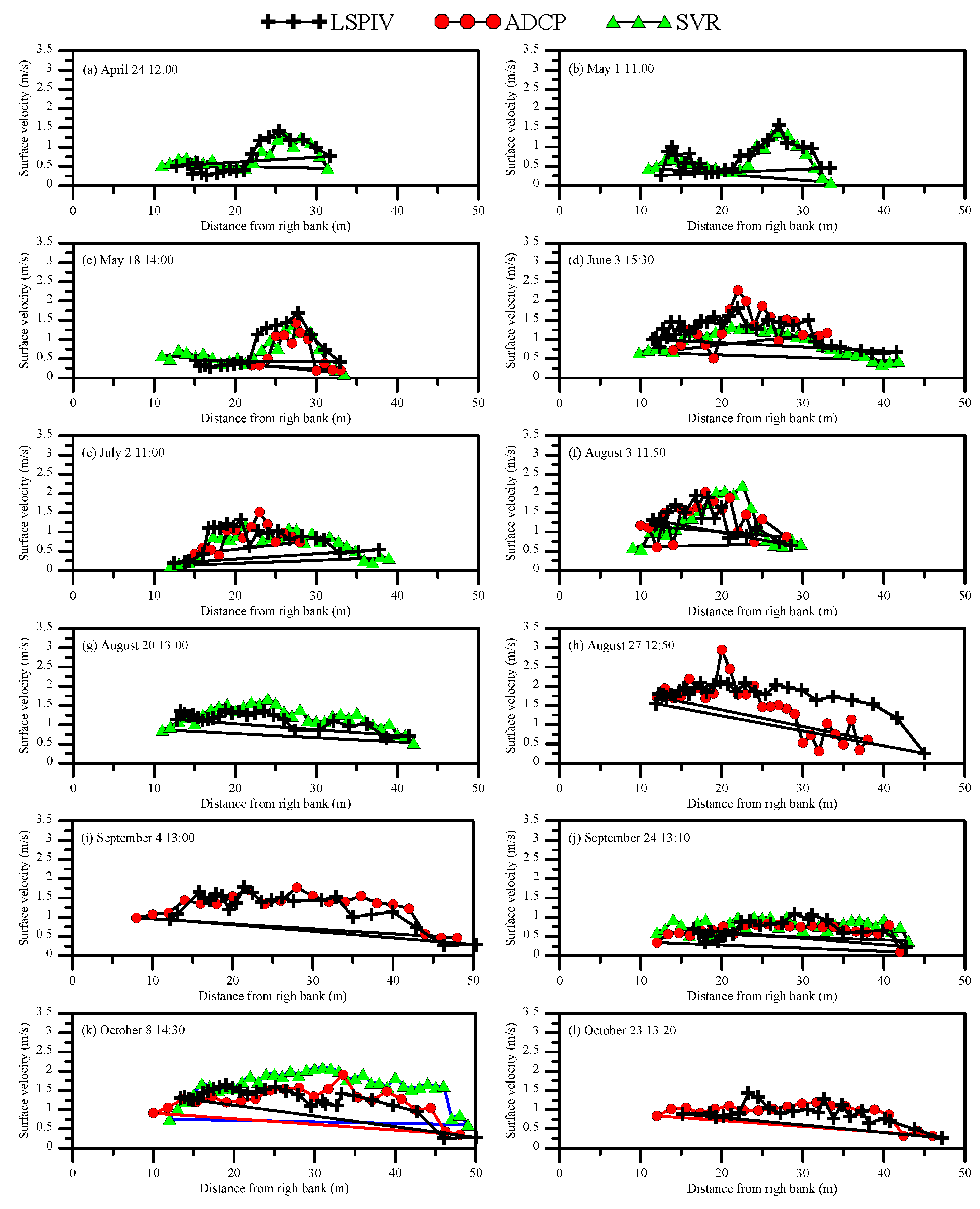
Figure 6 compares measured surface velocities along the channel cross-section in normal flow conditions. On each measured date, velocity patterns that were captured by LSPIV, ADCP, and SVR were quite consistent. From the right to the left river banks (i.e., the X axis in the figure), surface velocities close to both banks were smaller and gradually increased toward the central stream. During these periods, the maximum of surface velocity could reach 3 m/s approximately (see Figure 6h). Similar characteristics were also found in [8,20,27,28,29]. In terms of averaged surface velocity (shown in Table 2), differences between the ADIS/LSPIV and ADCP (or SVR) measurements range from 0.004 to 0.39 m/s (0.023 to 0.345 m/s).
Figure 7 shows a scatter plot for the averaged surface velocities from LSPIV and ADCP (or SVR) measurements. Also, the normalized root mean square error NRMSE, which is a statistical indicator, was used to quantify the accuracy, i.e.,
where N is the total number of data points; Oi is the measured results from ADCP (or SVR); Pi is the value measured with LSPIV. The NRMSE is 13.37% between LSPIV and ADCP measurements (or 6.75% when compared to SVR). Overall, comparisons indicated that ADIS/LSPIV is capable of measuring the surface velocities in river.
3.2. Comparison Surface Velocity and Water Level during Typhoon Event
ADIS based on LSPIV was further applied to measure surface velocities during typhoon events. Figure 8 presents the time series data for averaged surface velocities and self-recorded water depths at Yufeng gauging station during Typhoon Chan-Hom, Typhoon Soudelor, Typhoon Goni, and Typhoon Dujuan. In response to flash floods, both water depths and averaged surface velocities showed rapid increases. Especially, in the event of Typhoon Dujuan, the peak of averaged surface velocities up to 8 m/s was captured. The Froude numbers during measurement periods for Typhoon Chan-Hom, Typhoon Soudelor, Typhoon Goni, and Typhoon Dujuan are in the range of 0.6~1.05, 0.49~1.25, 0.48~0.56, and 0.34~1.04, respectively. We found that ADIS/LAPIV performed measurements well during a high Froude number. Noticed that no data were available in the nighttime currently since the ADIS would not work due to light limitation.
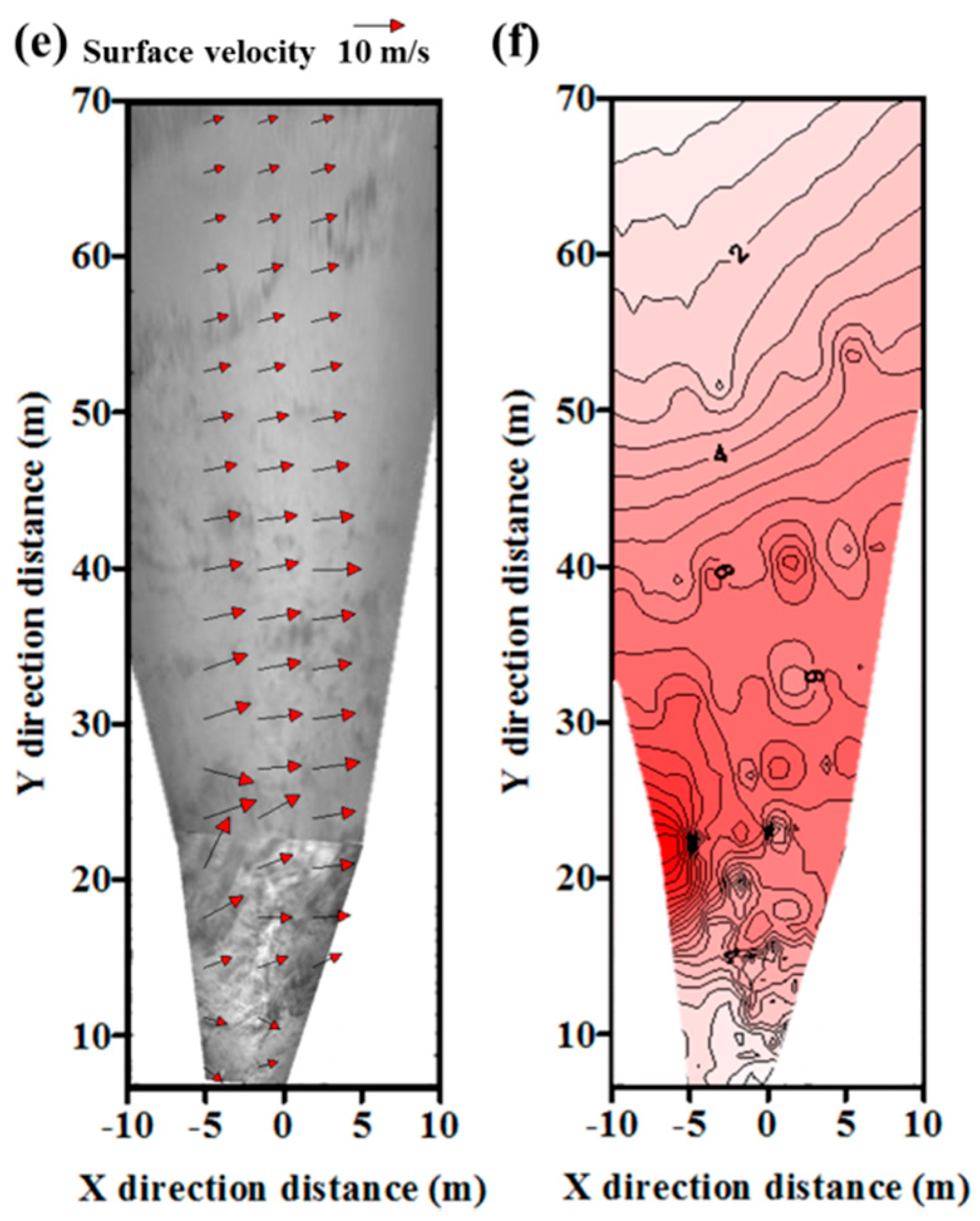
Figure 9 illustrates the velocity vectors and velocity contours using LSPIV on 28 September 2015 for Typhoon Dujuan. The value zero at X axis represents the camera location. Y axis is the lateral direction that represents across the river (see Figure 3). Because the river bank was flooded at 17:00, the river width at Y direction was extended when comparing to river width at 08:00 and 12:00. It also can be seen that the surface velocity at 17:00 is larger than that at 08:00 and 12:00. Because no measured data were collected using ADCP and SVR during typhoon events, the data in Figure 9 can not be reported in Figure 6 and Table 2.
Figure 10 shows the scatter plot for water depths and the averaged surface velocities in these four typhoon events, revealing a strong relationship with correlation coefficient R = 0.926. Similar results can be also found in the study of Creutin et al. [7] who conducted discharge measurement in the Iowa River using PIV techniques. Based on the high correlation, surface velocity of the flow was expressed as a function of water depth.
3.3. Index Velocity
Figure 11 compares the measured surface and depth-averaged velocities that were obtained at different dates. The surface velocity is measured from ADIS/LSPIV, while the depth-averaged velocity is obtained from ADCP measurement. Note that the cross-section area is calculated based on the actual water depth cross the river section, instead of assuming a constant averaged depth (see Figure 3d). Linear regression was used to yield the velocity-index relationship. The correction factor (velocity index) for Yu-Feng gauging station was k = 0.737 with a correlation coefficient R = 0.986. In the literature, Polatel [30] found that the velocity index ranges from 0.789 to 0.928 based on a series of laboratory experiments. Besides, Muste et al. [10] reported that the velocity index is dependent on the vertical profile of velocity affected by flow aspect ratio, Froude and Reynolds number, micro and macro bed roughness, and relative submergence of large-scale roughness elements. Le Coz et al. [20] utilized LSPIV approach to measure flash floods, giving a velocity index of 0.90 based upon available gauging data. By contrast, Jodeau et al. [8] considered a correction factor of k = 0.79 for a mountain stream under extreme flow conditions. In this study, the velocity index was 0.737, which is somewhat smaller but close to the value used in Jodeau et al. [8]. The reasonable explanation is that high bottom roughness (due to coverage of gravels and stones on the river bed) produces lower velocity index for the Yu-Feng Creek (at upper catchment of Shimen Reservoir).
3.4. Discharge Estimation
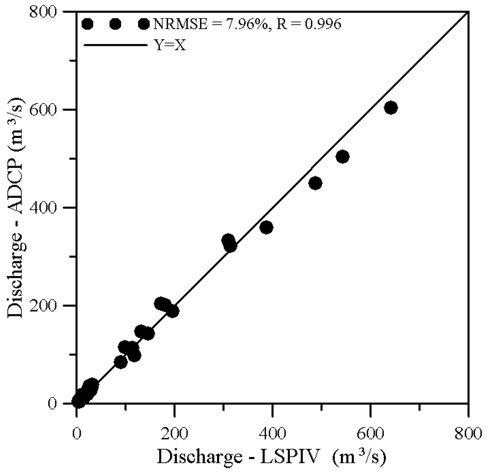
Discharge is calculated on the basis of the velocity-index and velocity-area methods. The measured surface velocity using LSPIV is transformed to depth averaged velocity, according to the velocity-index (shown in Figure 11). The depth averaged velocity multiplies by cross section area to yield the discharge. Figure 12 compares the estimated river discharges from ADIS/LSPIV and ADCP measurements. Good agreement (with R = 0.996 and NRMSE = 7.96%) indicates that the ADIS/LSPIV developed in this study provides a reliable tool for estimating flood discharge. Further, stream flows that were estimated using the conventional rating curve (from Water Resources Agency, Taiwan) are demonstrated in Figure 12. By comparison with the discharges from ADCP, flood estimations based on extrapolated part of the rating curve show significant credibility gaps [4], with a large statistical error of NRMSE = 42.2%.
The ADIS indirect flow measurement can be utilized to improve stage-discharge relationships and reduce uncertainties associated with flood discharges [31]. Later on, a combination with hydraulic analysis (from experimental investigation or numerical simulation) will be made to achieve further improvement for the LSPIV technique, e.g., capability in assessing various velocity structures over a range of flow conditions [20]. Overall, the results (see Figure 11 and Figure 12) indicated that the developed ADIS/LSPIV provides a promising, accurate, and robust alternative (or even a replacement to the conventional rating curve method) for estimating stream discharge over wide ranging flow conditions (especially in the mountainous cases like Taiwan) [20,32].
3.5. Sensitivity Analysis
The sensitivity analysis was conducted by varying the interior and exterior parameters at right and left cameras including uc, vc, d, xc, yc, zc, α, τ, and θ. The effect of each parameter at right and left cameras on the surface velocity using LSPIV was evaluated using two alternative cases, including 10% increase and 10% decrease in each parameter. The rate of change (RC) of surface velocity using LSPIV is given by following formula:
where Vsurf is the surface velocity obtained from LSPIV and Vsurf,sen is the surface velocity obtained from LSPIV according to sensitivity analysis of interior and exterior parameters at right and left cameras.
Table 1 illustrates the results of sensitivity analysis. It shows that two parameters τ and θ used in LSPIV technique are sensitive to the estimation of surface velocity. The increases in parameters τ and θ lead to a 49.67% decrease and an 84.11% increase in surface velocity, respectively. On the other hand, the decreases in parameters τ and θ yield a 294.75% increase and a 110.67% decrease for surface velocity, respectively. Given 10% change of surface velocity, the acceptable tolerances for parameters τ and θ are 0.8 and 3.5 degrees, respectively. In other words, one who measures the surface velocity using LSPIV should control the tilt (τ) and roll (θ) angles of camera within 0.8- and 3.5-degree deviation, respectively, in order to ensure effective measurement (i.e., less than 10% of error). We further deduced the uncertainty of measurement by specifying the parameters (τ = 0.8 degree and θ = 3.5 degree) with an increment of ±0.1 degree. In terms of τ (or θ), the resulting tolerance errors for surface velocity measurement were 10 ± 0.99% (or 10 ± 3.50%) under 95% confidence level. Note that the camera parameters should be carefully adjusted and calibrated to obtain accurate results. Once the positions of left/right cameras were shifted, the parameters must be re-calculated using the known control points to eliminate errors in surface velocity measurement.
4. Conclusions
In this study, the development of an automated discharge imaging system ADIS with LSPIV method for measuring flood discharges during typhoon events was presented. ADIS consists of dual cameras to capture complete surface images in the near and far fields. Surface velocities were accurately measured by the Large Scale Particle Image Velocimetry (LSPIV) technique. The ADIS/LSPIV was deployed at Yu-Feng gauging station in Shimen Reservoir upper catchment, northern Taiwan. For comparison (and validation), surface velocity measurements using ADIS/LSPIV and other instruments were carried out. All measured results were in good agreement with small differences in the averaged surface velocities, i.e., 0.004 to 0.39 m/s and 0.023 to 0.345 m/s when compared the ADIS/LSPIV to acoustic Doppler current profiler (ADCP) and surface velocity radar (SVR), respectively. The ADIS/LSPIV was further utilized to measure surface velocity during typhoon events in 2015. The measured water level and surface velocity were highly correlated, showing rapid changes simultaneously in response to flash floods.
The river discharge was calculated using a velocity-index approach that transfers the surface velocity that was obtained from LSPIV to a depth-averaged one. Due to coverage of gravels and stones on the river bed, high bottom roughness led to a small correction factor k = 0.737 in the Yu-Feng Creek. The stream discharge was also estimated from ADCP measurement results using the velocity-area method. Discharges obtained from ADIS/LSPIV and ADCP were quite comparable with R = 0.996 and NRMSE = 7.96%. Conventional flood estimation based upon extrapolated parts of a rating curve yielded significant credibility gaps with a large statistical error of NRMSE = 42.2%. The sensitivity analysis of parameter shows that components till (τ) and roll (θ) of the camera are the most sensitive parameter to affect the surface velocity using LSPIV technique. Overall, the promising ADIS/LSPIV provides non-intrusive, safe, and reliable measurement to obtain river discharges during flood events.
The limitation of ADIS/LSPIV indeed requires preliminary field-based intrusive experimental campaign for image calibration and the ADCP measurements for estimating the depth. The ADIS/LSPIV measurement in the nighttime would be supplied with an extra light source, which should be investigated and resolved.
In field experiments, despite its great performance, the ADIS/LSPIV technique for stream discharge measurement may still encounter uncertainties from various factors, such as orthorectification induced by camera movement, image quality and sampling, surface velocity errors affected by wind and trace quality, and complex flow structures. In the future study, field measurements will be investigated to assess uncertainties in the ADIS/LSPIV and to evaluate the sensitivity of the LSPIV for turbulent flow.
Acknowledgments
This study was supported by the Northern Region Water Resources Office, Water Resources Agency, Taiwan, under grant No. 104C10. This financial support is greatly appreciated. The authors acknowledge two anonymous reviewers provided useful comments and suggestions for improving the manuscript.
Author Contributions
Wen-Cheng Liu supervised the progress of the Water Resources Agency’s project, served as a general editor, and prepared a draft of the manuscript. Wei-Che Huang and Chih-Chieh Young performed the experiments, data collection and analysis, and model establishment and discussed the results with Wen-Cheng Liu. All authors read and approved the final manuscript.
Conflicts of Interest
The authors declare no conflict of interest.
References
- Buchanan, T.J.; Somers, W.P. Discharge measurements at gauging station: U.S. geological survey techniques of water-resources investigations. In Technical Reports; U.S. Geological Survey: Reston, VA, USA, 1969. [Google Scholar]
- Tauro, F.; Selker, J.; van de Giesen, N.; Abrate, T.; Uijlenhort, R.; Porfiri, M.; Manfreda, S.; Caylor, K.; Moramarco, T.; Benveniste, J.; et al. Measurements and observations in the XXI century (MOXXI): Innovation and multidisciplinary to sense the hydrological cycle. Hydrol. Sci. J. 2018, 63, 169–196. [Google Scholar] [CrossRef]
- Rantz, S.E. Measurement and computation of streamflow. Measurement of Stage and Discharge. In Water-Supply Paper 2175; U.S. Geological Survey: Washington, DC, USA, 1982; Volume 1. [Google Scholar]
- Lang, M.; Ponanz, K.; Renard, B.; Renouf, E.; Sauquet, E. Extrapolation of rating curves by hydraulic modeling, with application to flood frequency analysis. Hydrol. Sci. J. 2010, 55, 883–989. [Google Scholar] [CrossRef]
- Coata, J.; Cheng, R.; Haeni, F.; Melcher, N.; Spicer, K.; Hayes, E.; Plant, W.; Hayes, K.; Teague, C.; Barrick, D. Use of radars to monitor stream discharge by noncontact method. Water Resour. Res. 2006, 40, 14. [Google Scholar]
- Fujita, I.; Muste, M.; Kruger, A. Large-scale particle image velocimetry for flow analysis in hydraulic engineering applications. J. Hydraul. Res. 1998, 36, 397–414. [Google Scholar] [CrossRef]
- Creutin, J.D.; Muste, M.; Bradley, A.A.; Kim, S.C.; Kruger, A. River gauging using PIV techniques: A proof of concept experiment on the Iowa River. J. Hydrol. 2003, 277, 182–194. [Google Scholar] [CrossRef]
- Jodeau, M.; Hauet, A.; Paquier, A.; Le Coz, J.; Dramais, G. Application and evaluation of LS-PIV technique for the monitoring river surface velocities in high flow conditions. Flow Meas. Instrum. 2008, 19, 117–127. [Google Scholar] [CrossRef] [Green Version]
- Hauet, A.; Kruger, A.; Krajewski, W.F.; Bradley, A.; Muste, M.; Creutin, J.D. Experiment system for real-time discharge estimation using an imagine-based method. J. Hydrol. Eng. 2008, 13, 105–110. [Google Scholar] [CrossRef]
- Muste, M.; Fujita, I.; Hauet, A. Large-scale particle image velocimetry for measurements in riverine environments. Water Resour. Res. 2008, 44. [Google Scholar] [CrossRef]
- Sun, X.; Shiono, K.; Chandler, J.H.; Rameshwaran, P.; Sellin, H.J.; Fujita, I. Discharge estimation in small irregular river using LSPIV. Proc. Inst. Civ. Eng. Water Manag. 2010, 163, 247–254. [Google Scholar] [CrossRef] [Green Version]
- Tsubaki, R.; Fujita, I.; Tsutsumi, S. Measurement of the flood discharge of a small-sized river using an existing digital video recording system. J. Hydro-Environ. Res. 2011, 5, 313–321. [Google Scholar] [CrossRef]
- Bechle, A.; Wu, C.H.; Liu, W.C.; Kimura, N. Development and application of an automated river-estuary discharge imaging system. J. Hydraul. Eng. ASCE 2012, 138, 27–339. [Google Scholar] [CrossRef]
- Dobson, D.W.; Holland, K.T.; Calantoni, J. Fast, large-scale, particle image velocimetry-based estimations of river surface velocity. Comput. Geosci. 2014, 70, 35–43. [Google Scholar] [CrossRef]
- Tauro, F.; Olivieri, G.; Petroselli, A.; Porfiri, M.; Grimaldi, S. Flow monitoring with a camera: A case study on a flood event in the Tiber River. Environ. Monit. Assess. 2016, 188, 118. [Google Scholar] [CrossRef] [PubMed]
- Tauro, F.; Petroselli, A.; Porfiri, M.; Giandomenico, L.; Bernardi, G.; Mele, F.; Spina, D.; Grimaldi, S. A novel permanent gauge-cam station for surface-flow observations on the Tiber River. Geosci. Instrum. Methods Data Syst. 2016, 5, 241–251. [Google Scholar] [CrossRef]
- Tauro, F. Particle tracers and image analysis for surface flow observations. WIREs Water 2016, 3, 25–39. [Google Scholar] [CrossRef]
- Hauet, A.; Muste, M.; Ho, H.C. Digital mapping of riverine waterway hydrodynamic and geomorphic features. Earth Surf. Proc. Land. 2009, 34, 242–252. [Google Scholar] [CrossRef]
- Kantoush, S.A.; Schleiss, A.J. Channel formation during flushing of large shallow reservoirs with different geometries. Environ. Technol. 2009, 30, 855–863. [Google Scholar] [CrossRef] [PubMed]
- Le Coz, J.; Hauet, A.; Pierrefeu, G.; Dramais, G.; Camenen, B. Performance of imagine-based velocimetry (LSPIV) applied to flash-flood discharge measurements in Mediterranean rivers. J. Hydrol. 2010, 394, 542–552. [Google Scholar] [CrossRef]
- Wanek, J.M.; Wu, C.H. Automated trinocular stereo imaging system for three-dimensional surface wave measurements. Ocean Eng. 2006, 33, 723–747. [Google Scholar] [CrossRef]
- Wolf, P.; DeWitt, B. Elements of Photogrammetry: With Applications in GIS; McGraw-Hill: Boston, MA, USA, 2000. [Google Scholar]
- Holland, K.T.; Holman, R.A.; Lippmann, T.C.; Stanley, J.; Plant, N. Practical use of video imagery in nearshore oceanographic field studies. IEEE J. Ocean. Eng. 1997, 22, 81–92. [Google Scholar] [CrossRef]
- Mei, C.C. The Applied Dynamics of Ocean Surface; World Science: Singapore, 1989. [Google Scholar]
- Harpold, A.A.; Mostaghimi, S.; Vlachos, P.P.; Brannan, K.; Dillaha, T. Stream discharge measurement using Large-Scale Particle Image Velocimetry (LSPIV) prototype. Trans. ASABE 2006, 49, 1791–1805. [Google Scholar] [CrossRef]
- Herschy, R. Streamflow Measurement; Taylor & Francis: New York, NY, USA, 2009. [Google Scholar]
- Gunawan, B.; Sun, X.; Sterlingm, M.; Shiono, K.; Tsubaki, R.; Rameshwaran, P.; Knight, D.W.; Chandler, J.H.; Yang, X.; Fujita, I. The application of LS-PIV to a small irregular river for inbank and overbank flows. Flow Meas. Instrum. 2012, 24, 1–12. [Google Scholar] [CrossRef] [Green Version]
- Daigle, A.; Berube, F.; Bergeron, N.; Matte, P. A methodology based on particle image velocimetry for river ice velocity measurement. Cold Reg. Sci. Technol. 2013, 89, 36–47. [Google Scholar] [CrossRef]
- Patalano, A.; Garcia, C.M.; Brevis, W.; Bleninger, T.; Guillen, N.; Moreno, L.; Rodriguez, A. Recent advances in Eulerian and Lagragian large-scale particle image velocimetry. In Proceedings of the 36th IAHR World Congress, The Hague, The Netherlands, 26 June–3 July 2015; pp. 1–6. [Google Scholar]
- Polatel, C. Indexing free-surface velocity. In Proceedings of the a Prospect for Remote Discharge Estimation, Paper Presented at 31st Congress, International Association of Hydraulic Engineering and Research, Seoul, Korea, 11–16 September 2005. [Google Scholar]
- Dramais, G.; Le Coz, J.; Camenen, B.; Hauet, A. Advantages of a mobile LSPIV method for measuring flood discharges and improving stage-discharge curves. J. Hydro-Environ. Res. 2011, 5, 301–312. [Google Scholar] [CrossRef]
- Muste, M.; Ho, H.C.; Kim, D. Consideration on direct stream flow measurements using video imagery: Outlook and research needs. J. Hydro-Environ. Res. 2011, 5, 289–300. [Google Scholar] [CrossRef]
Figure 1.
Location map of the study site. The Yufeng Creek is an upstream tributary of the Dahan River.
Figure 1.
Location map of the study site. The Yufeng Creek is an upstream tributary of the Dahan River.
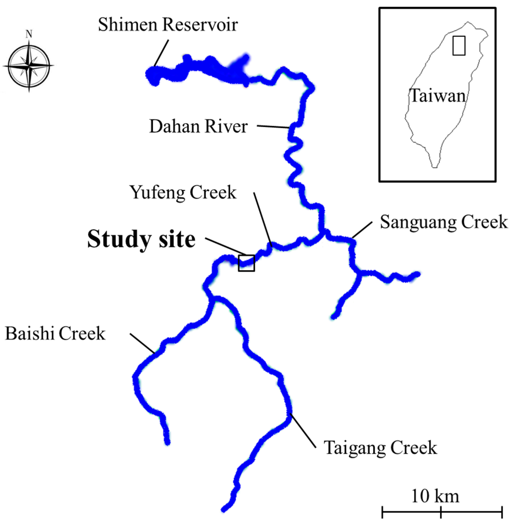
Figure 2.
The far- and near-field photos obtained from the dual cameras: (a,b) for the normal flow condition; (c,d) for Typhoon Soudelor in August 2015.
Figure 2.
The far- and near-field photos obtained from the dual cameras: (a,b) for the normal flow condition; (c,d) for Typhoon Soudelor in August 2015.

Figure 3.
(a) Illustration for the near-field and far-field camera view angles at Yufeng gauging station. Note that the acoustic Doppler current profile (ADCP) and surface velocity radar (SVR) data acquisition campaign along the river is also shown in the figure, (b) cross section of the river (from right bank to left bank), (c) picture of the control points, and (d) measured locations of control points in a horizontal plane during image calibration.
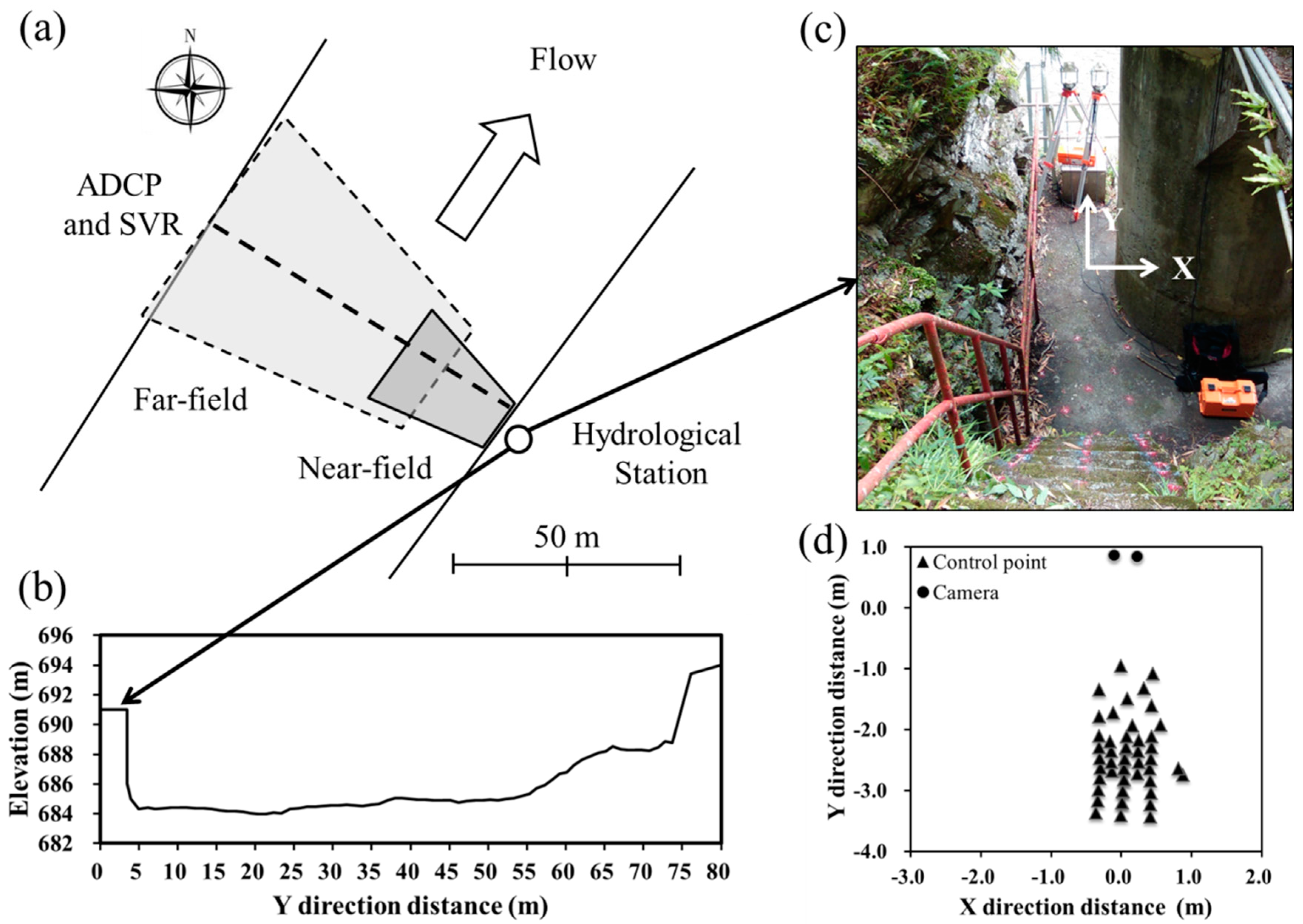
Figure 4.
The automated discharge imaging system (ADIS) hardware system consists of two cameras, both enclosed in the weatherproof cases.
Figure 4.
The automated discharge imaging system (ADIS) hardware system consists of two cameras, both enclosed in the weatherproof cases.

Figure 5.
The collinearity relationship between the object (x, y, z), image point (u, v), and camera (xc, yc, zc). Note that ∆α is the change of angle from the initial azimuth α to the observation area.
Figure 5.
The collinearity relationship between the object (x, y, z), image point (u, v), and camera (xc, yc, zc). Note that ∆α is the change of angle from the initial azimuth α to the observation area.

Figure 6.
Comparison of surface velocities measured by LSPIV, ADCP, and SVR on different dates under normal flow conditions: (a) 24 April, (b) 1 May, (c) 18 May, (d) 3 June, (e) 2 July, (f) 3 August, (g) 20 August, (h) 27 August, (i) 4 September, (j) 24 September, (k) 8 October, and (l) 23 October in the year of 2015.

Figure 7.
Scatter plot of averaged surface velocities for Large Scale Particle Image Velocimetry (LSPIV) against SVR (solid circles) and ADCP (open circles) measurements.
Figure 7.
Scatter plot of averaged surface velocities for Large Scale Particle Image Velocimetry (LSPIV) against SVR (solid circles) and ADCP (open circles) measurements.
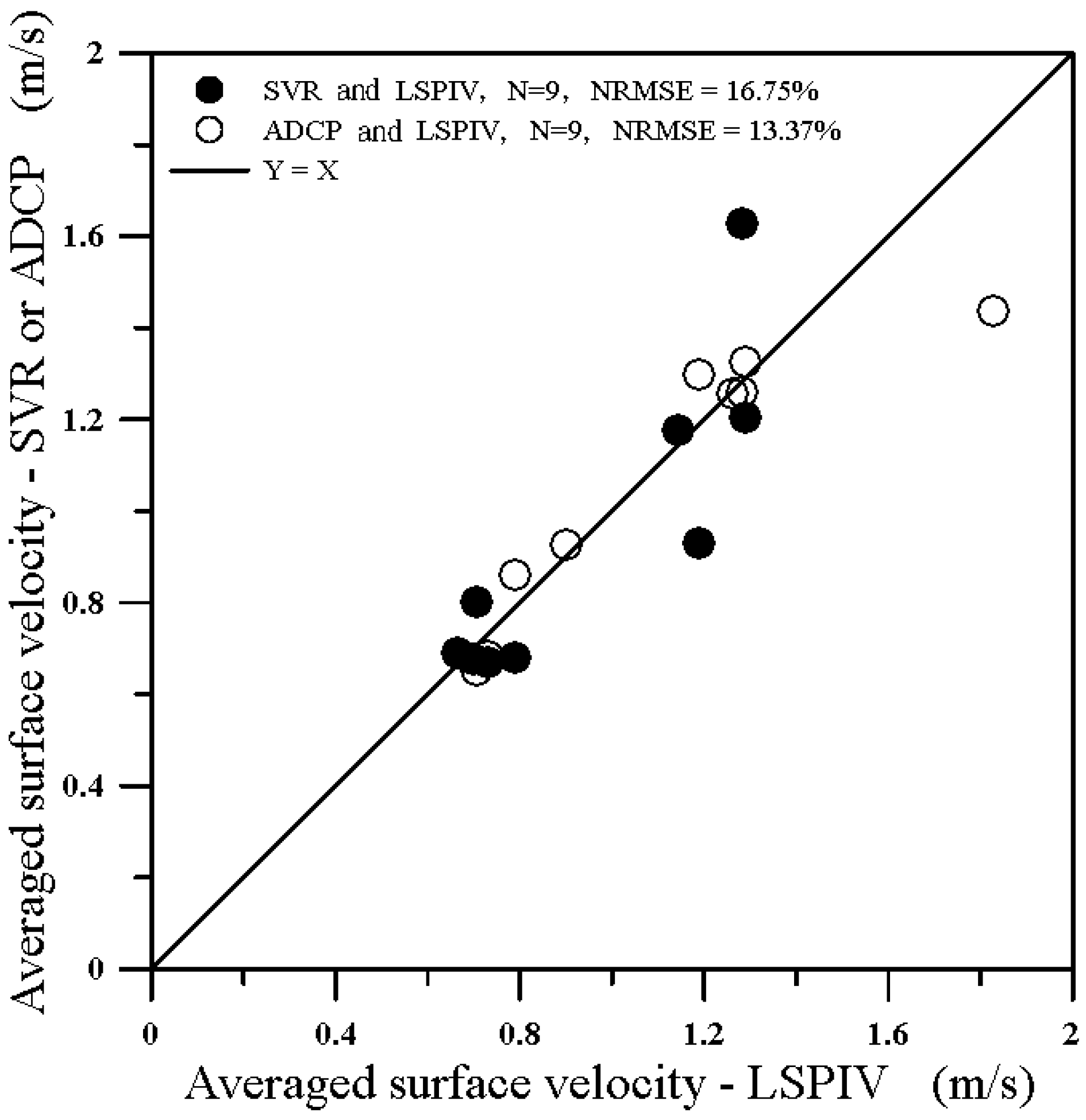
Figure 8.
Time series data of self-recorded water levels and averaged surface velocities obtained by LSPIV at the Yufeng gauging station during (a) Typhoon Chan-Hom, (b) Typhoon Soudelor, (c) Typhoon Goni, and (d) Typhoon Dujuan in the year of 2015.
Figure 8.
Time series data of self-recorded water levels and averaged surface velocities obtained by LSPIV at the Yufeng gauging station during (a) Typhoon Chan-Hom, (b) Typhoon Soudelor, (c) Typhoon Goni, and (d) Typhoon Dujuan in the year of 2015.
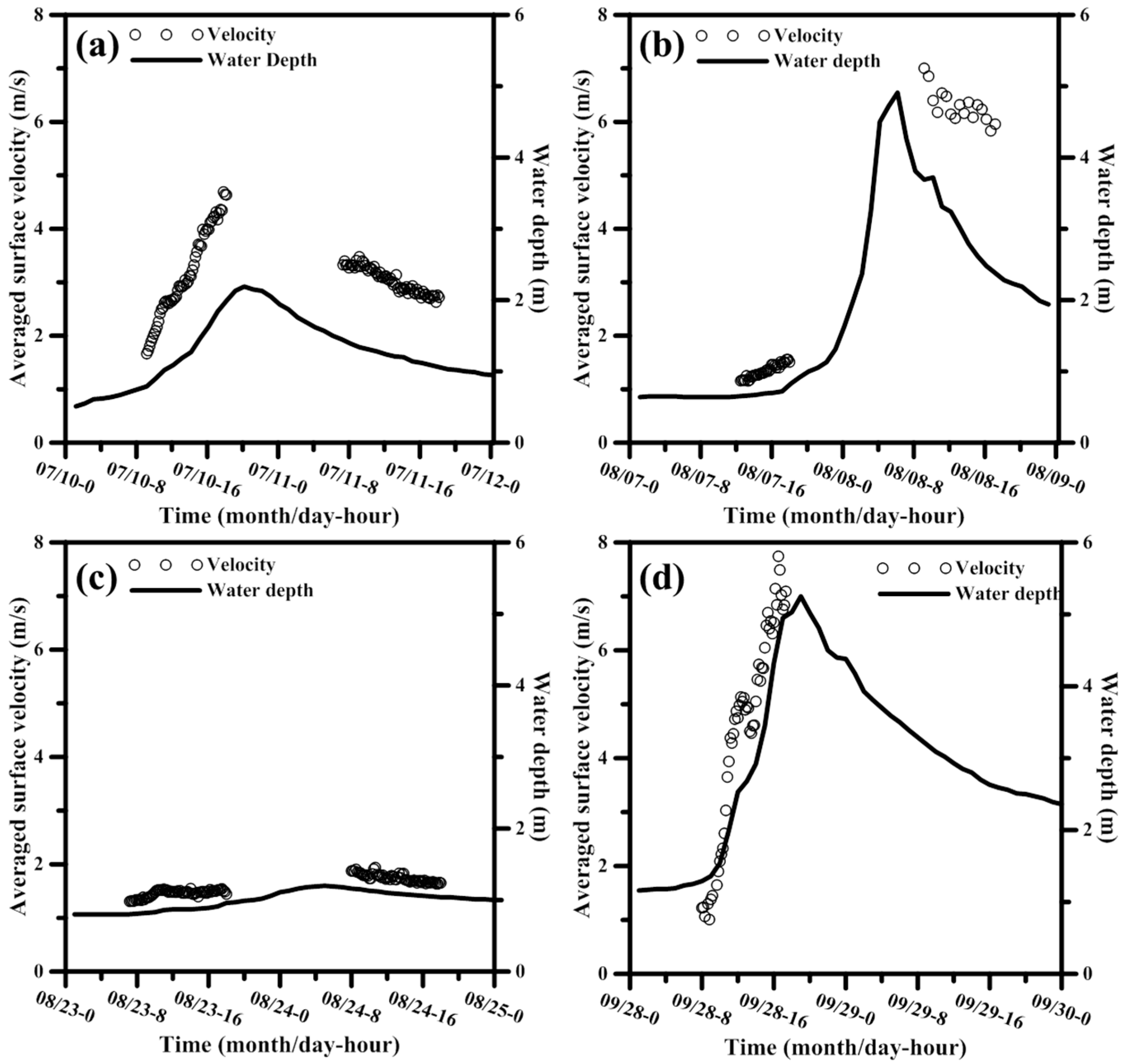
Figure 9.
Measured surface velocity using LSPIV on 28 September 2015 (Typhoon Dujuan) (a) velocity vector at 08:00, (b) velocity contour at 08:00, (c) velocity vector at 12:00, (d) velocity contour at 12:00, (e) velocity vector at 17:00, and (f) velocity contour at 17:00.
Figure 9.
Measured surface velocity using LSPIV on 28 September 2015 (Typhoon Dujuan) (a) velocity vector at 08:00, (b) velocity contour at 08:00, (c) velocity vector at 12:00, (d) velocity contour at 12:00, (e) velocity vector at 17:00, and (f) velocity contour at 17:00.
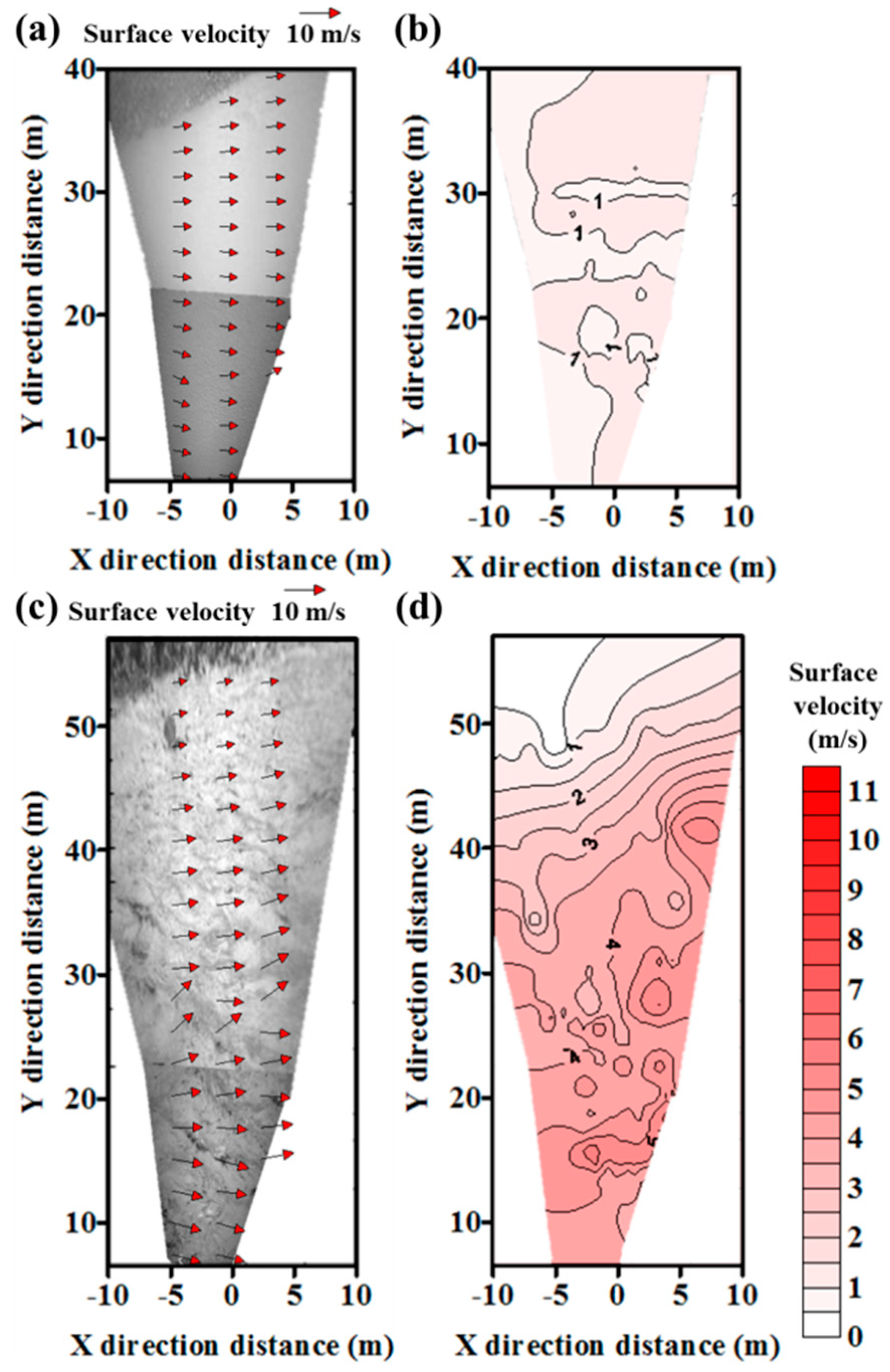

Figure 10.
Scatter plot between measured water depths and averaged surface velocities for all typhoon events in 2015.
Figure 10.
Scatter plot between measured water depths and averaged surface velocities for all typhoon events in 2015.
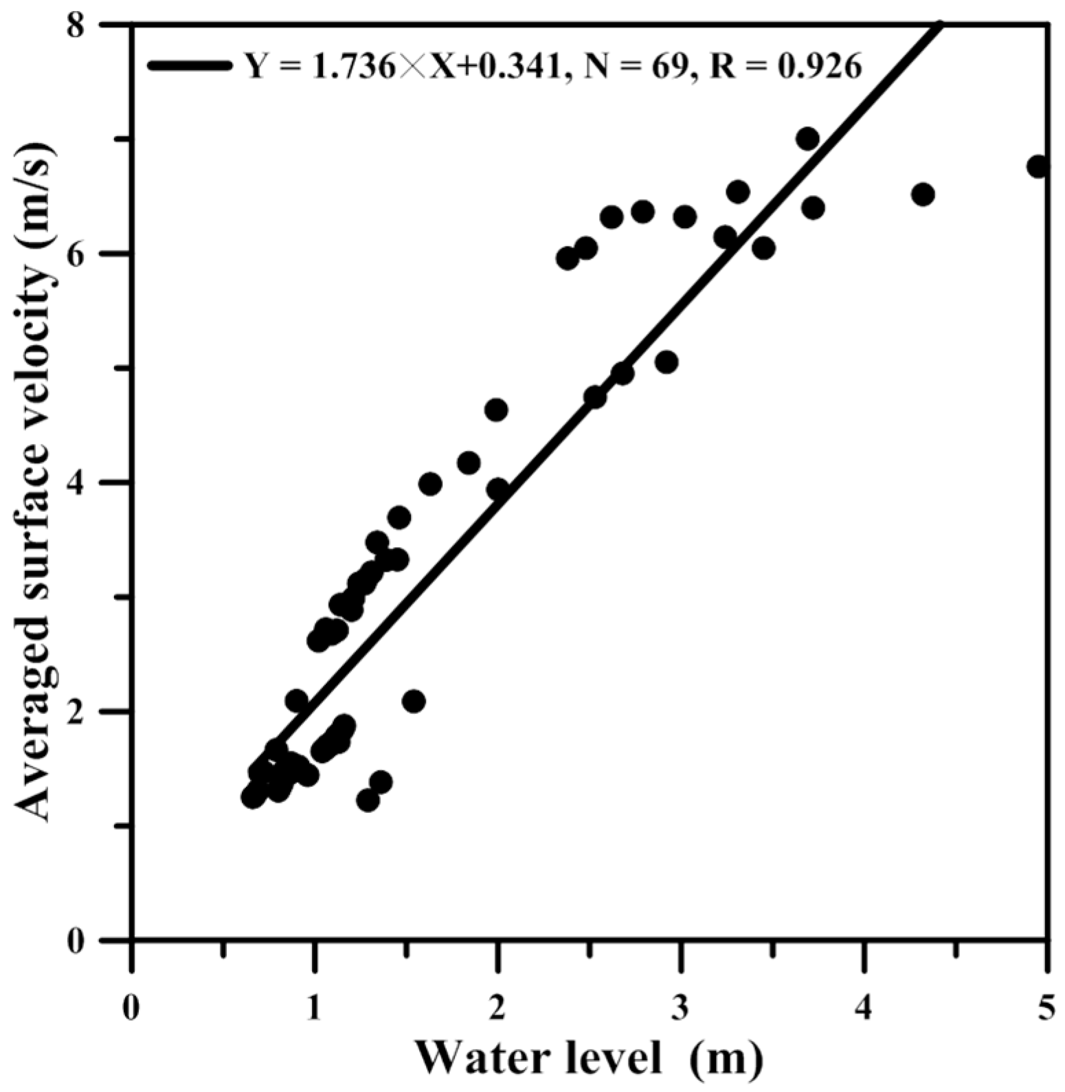
Figure 11.
The velocity-index relationship between LSPIV averaged surface velocity and depth-averaged velocity.
Figure 11.
The velocity-index relationship between LSPIV averaged surface velocity and depth-averaged velocity.
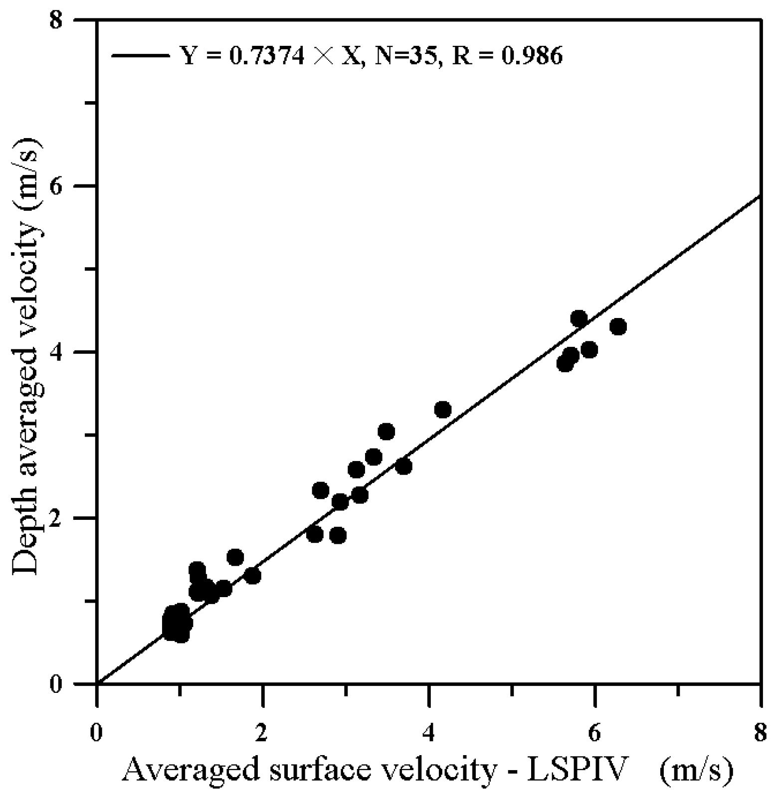
Figure 12.
Comparison of estimated river discharge from the ADIS/LSPIV and ADCP measurements.


Table 1.
Parameters used for right and left cameras and results of parameter sensitivity analysis.
| Parameter | Right Camera | Left Camera | Rate of Change (RC) of Surface Velocity Using LSPIV (%) | |
|---|---|---|---|---|
| Parameter Used at Right and Left Cameras Increases 10% | Parameter Used at Right and Left Cameras Decreases 10% | |||
| uc (pixel) | 800 | 800 | −0.56 | 0.57 |
| vc (pixel) | 600 | 600 | 10.14 | −7.67 |
| d (m) | 0.0147 | 0.0168 | −7.77 | 10.44 |
| α (degree) | 2.44 | −1.98 | 0.00 | 0.00 |
| τ (degree) | 115.86 | 98.22 | −49.67 | 294.75 |
| θ (degree) | 178.15 | 178.94 | 84.11 | −110.67 |
| xc (m) | 0.230 | −0.091 | 0.00 | 0.00 |
| yc (m) | 1.056 | 1.622 | 0.00 | 0.00 |
| zc (m) | 1.785 | 1.738 | 2.23 | −2.23 |
Table 2.
Averaged surface velocities from ADIS, ADCP, and SVR measurements.
| Measured Date in Year 2015 | Averaged Surface Velocity (m/s) | ||||
|---|---|---|---|---|---|
| LSPIV (A) | ADCP (B) | SVR (C) | |||
| 24 April, 12:00 | 0.663 | -- | 0.691 | -- | 0.028 |
| 1 May, 11:00 | 0.698 | -- | 0.675 | -- | 0.023 |
| 18 May, 14:00 | 0.73 | 0.682 | 0.67 | 0.048 | 0.06 |
| 3 June, 15:30 | 1.189 | 1.3 | 0.929 | 0.111 | 0.26 |
| 2 July, 11:00 | 0.79 | 0.861 | 0.679 | 0.071 | 0.111 |
| 3 August, 11:50 | 1.291 | 1.325 | 1.206 | 0.034 | 0.085 |
| 20 August, 13:00 | 1.144 | -- | 1.178 | -- | 0.034 |
| 27 August, 12:50 | 1.827 | 1.437 | -- | 0.39 | -- |
| 4 September, 13:00 | 1.26 | 1.256 | -- | 0.004 | -- |
| 24 September, 13:10 | 0.706 | 0.654 | 0.8 | 0.052 | 0.094 |
| 8 October, 14:30 | 1.283 | 1.26 | 1.628 | 0.023 | 0.345 |
| 23 October, 13:20 | 0.9 | 0.928 | -- | 0.028 | -- |
© 2018 by the authors. Licensee MDPI, Basel, Switzerland. This article is an open access article distributed under the terms and conditions of the Creative Commons Attribution (CC BY) license (http://creativecommons.org/licenses/by/4.0/).
Share and Cite
MDPI and ACS Style
Huang, W.-C.; Young, C.-C.; Liu, W.-C. Application of an Automated Discharge Imaging System and LSPIV during Typhoon Events in Taiwan. Water 2018, 10, 280. https://doi.org/10.3390/w10030280
AMA Style
Huang W-C, Young C-C, Liu W-C. Application of an Automated Discharge Imaging System and LSPIV during Typhoon Events in Taiwan. Water. 2018; 10(3):280. https://doi.org/10.3390/w10030280
Chicago/Turabian StyleHuang, Wei-Che, Chih-Chieh Young, and Wen-Cheng Liu. 2018. "Application of an Automated Discharge Imaging System and LSPIV during Typhoon Events in Taiwan" Water 10, no. 3: 280. https://doi.org/10.3390/w10030280
Note that from the first issue of 2016, this journal uses article numbers instead of page numbers. See further details here.