The Influence of Climate Variability Effects on Groundwater Time Series in the Lower Central Plains of Thailand

1
Department of Civil Engineering, Faculty of Engineering, King Mongkut’s Institute of Technology Ladkrabang, Bangkok 10520, Thailand
2
Groundwater Research Center, Faculty of Technology, Khon Kaen University, Khon Kaen 40002, Thailand
*
Author to whom correspondence should be addressed.
Water 2018, 10(3), 290; https://doi.org/10.3390/w10030290
Submission received: 24 January 2018
/
Revised: 5 March 2018
/
Accepted: 5 March 2018
/
Published: 8 March 2018
Abstract
:This research studies the relationship between the climate index and the groundwater level of the lower Chao Phraya basin, in order to forecast the groundwater level in the studied area by using Autoregressive Integrated Moving Average with Explanatory (ARIMAX). The combination of 6 climate indices—Dipole Mode Index, Indian Summer Monsoon Index, Multivariate ENSO Index, Sea Surface Temperature NINO4, Southern Oscillation Index and the Western North Pacific Monsoon Index—were used, along with the groundwater level data from 14 stations during the period 1980–2011 to develop the forecast model and verify it with the data of 2012.The first step was correlation of the ARIMA model with Autocorrelation Function and Partial Autocorrelation Function. The possible model was then selected using BIC statistics. Diagnostic Checking was done to consider the white noise characteristic of estimated residuals by using the statistics of Box and Ljung (Q-statistic). If the selected models were found to be proper, then the Granger Causality Test of the leading parameters or the climate index would be performed as the next step. The results show that there is a relationship between the groundwater level and the climate index. The model could be used to forecast effectively the average RMSE value at 0.6. The last step was to develop the MODFLOW for a conceptual model and synthesize groundwater levels in the study area, which covers around 43,000 km2 and has 8 layers of groundwater, with Bangkok clay on the top. All other boundary values were set to be steady. The calibration was done using the data of 325 observed wells. The normalized RMS value was 9.705%. The results were verified by the data using ARIMAX over the same time periods. To conclude, the simulated results of the monthly groundwater level in 2012 of the wells have a confidence interval of around 95%, which is near the result from the ARIMAX model. The advantages of the ARIMAX model include high accuracy, no requirement for a large amount of data and inexpensive implementation. It is one of the effective tools for the groundwater prediction.
1. Introduction
As is widely known, the world’s weather is currently facing global changes [1], which can be seen from the variability of weather and changes in the climate in many parts of the world [2]. Every aspect is involved in this climate variability, including atmosphere, ocean levels and average temperature, resulting in changes in season timing and rain distribution [3]. The studies of the Intergovernmental Panel on Climate Change (IPCC) in 2001 [4] showed that the average world temperature had increased by 1.4 to 5.8 degrees Celsius. This resulted in the melting of polar ice and the expansion of the ocean area, the increase of sea level by at least 0.09 m to 0.88 m and variability in the distribution of rain, which could result in both more severe drought and flooding.
Thailand, which is located in the Southeast Asia region, is affected by the climate variability caused by the interaction between the ocean, atmosphere and the ground in the equatorial area between the Indian Ocean and the Pacific Ocean. Two important climate variability phenomena in this area are the Indian Ocean Dipole (IOD) and the El Nino–Southern Oscillation (ENSO). Therefore, the study of climate variability to understand the effect on water resources and the preparation of water management is definitely an essential activity.
Groundwater is one of the most important water resources for billions of people, especially for many developing countries in Asia. Groundwater use accounts for about 50 percent of consumed water, 40 percent of all industrial water usage and 20 percent of agricultural water usage. In Asia-Pacific, approximately 32 percent of the population uses groundwater as drinking water [5]. More than 2 million people in Asia use only groundwater for consuming. In some countries, such as Bangladesh, India, China, Indonesia, the Philippines, Thailand and Vietnam, more than 50 percent of households use groundwater [6]. Furthermore, in most of the big cites, groundwater has been used more for industry than consumption. In Bangkok, the groundwater accounts for about 60 percent of all water used in industry, so the quantity of groundwater used is related to Gross Domestic Product (GDP). All of the above factors could affect the overall quantity of groundwater.
The objectives of this paper are to find the relationship between climate variability and groundwater by comparing groundwater level results when analyzed and forecasted using two models. The ARIMAX model is used to forecast the groundwater level with the exogenous climate index variable. The result of the ARIMAX model is used in comparison with the result from the groundwater level in the study area analyzed by the MODFLOW model. The Chao Phraya River basin is the largest groundwater basin in Thailand, which is one of the most important industrial areas and high residential population areas of Thailand, covering 15 provinces, and it is the focus of this study. Understanding the connection between climate variability and groundwater could lead to better knowledge about groundwater levels, better preparation, development and management of natural resources and the ability to lessen the sensitivity of people to climate change.
2. Linkages between Climate Variability and Water Resources
Worldwide, people’s water resources respond to climate variability very quickly. Regional climates are affected by many forms of climate variability. The one that is most well-known is the El Nino–Southern Oscillation (ENSO) [7]. Moreover, variations in the phenomena were found in decade-long spans such as Pacific Decadal Oscillation (PDO) [8,9], the North Atlantic Oscillation (NAO) [10] and the Atlantic Multidecadal Oscillation (AMO) [11].
Previous studies have shown the relationship between rainfall and climate variability in many areas throughout the world, such as in Queensland by Chiew et al. [12] and in the southwestern region of the United States by Hanson et al. [2]. Thailand has been affected by the difference in climate from both the Indian and Pacific Ocean. Yearly rainfall decreases in El Nino years and increases in the La Nina years [13]. The relationship between climate index and change of multi-year rainfall, up to decades, was researched and found by Kusreesakul [14], Limsakul and Goes [15]. The variations in the world’s climate have also impacted surface water resources and groundwater resources in Thailand. Limsakul et al. [16] has found that the yearly raining period is related to the Indian Ocean Monsoon Index (IMI) and the Western North Pacific Monsoon Index (WNPMI).
In the future, water use will rely on groundwater more because of the quickly changing and unreliable surface water level. In many areas, the surface water level is forecast to become more variable, which could drop the quality of surface water because of more severe drought and more frequent rain [17]. In the IPCC report, current surface water management is not sufficient to ensure the quantity of tap water impacted by climate change. Therefore, the number of wells is increasing very quickly [18] because farmers rely on it more and the surface water supply will be unreliable due to climate change.
Although the number of journal publications per year and the cumulative number of papers about the impact of climate change on ground water resources from 1990 to 2010 had largely increased [1], more research is still needed urgently to define conjunctive use adaptation strategies to improve the management of groundwater [19], under the impact of world climate change and variation [20]. Studying the probable impact of climate change on groundwater variation is much more complex than the impact on the surface water [21]. The groundwater could have a lifetime from a few days to a hundred thousand years. Although groundwater could slow down the impact from climate change, the impact on the groundwater is difficult to monitor and detect [22]. Moreover, many activities caused by humans, such as pumping up the groundwater, could affect the groundwater in the same period as the climate change, which makes the differentiation of impact from climate change and human activity more complex. USGS has tried to study the groundwater level hydrology and agronomical chemistry response signal in the interannual to multidecadal time scales because this time scale variation could be highly significant for groundwater resource management [2,23,24,25].
The main interest of groundwater and the climate change research is the forecasting and estimation of probable direct impact on the rainfall variation and temperature formation [26,27,28]. These studies could be simulated by different models, such as the water and soil equilibrium model [28,29], Empirical model [30], conceptual model [31] and complex distribution model [32,33]. In addition, Changnon et al. [34] have studied the relationship between monthly precipitation (P) and the shallow groundwater level (GW) in 20 wells scattered across the American state of Illinois using autoregressive integrated moving average (ARIMA) modeling. The model found that a lag of 1 month between P to GW has the strongest temporal relationship found across Illinois, followed by no (0) lag in the northern two-thirds of Illinois, where mollisols predominate and a lag of 2 months in the alfisols of southern Illinois. Adhikary et al. [35] also used ARIMA to simulate the fluctuation of the groundwater table of all monitored wells in the Kushtia district of Bangladesh. The results show that the predicted data represented the actual data very well for each monitored well. Furthermore, groundwater heads at a confined aquifer in southwest Florida show a nonstationary long-term (multi-year) fluctuation. Ahn and Salas [36] introduced an approach to build a time series models of nonstationary data at different time intervals based on an observed time series sampled at a reference interval. The model utilized in their study was a first-order difference ARIMA model. However, some groundwater head data may also be fitted adequately by a second-order difference time series model [37]. Five-time series models were applied: autoregressive (AR), moving average (MA), auto-regressive moving-average (ARMA), autoregressive integrated moving-average (ARIMA) and seasonal auto-regressive integrated moving-average (SARIMA). The results showed that the AR model with a two-time lag (AR(2)) shows the best forecasting of groundwater level. However, they should be combined with several time series models for a better prediction of groundwater level [38].
The MODFLOW model, which was developed by the U.S. Geological Survey, is widely used for groundwater modelling [39]. Visual MODFLOW was then developed by Waterloo Hydrogeologic, Inc. (Kitchener, ON, Canada) to help prepare the data and conveniently display the groundwater model. For instance, Lawrence et al. [40] used MODFLOW for the hydrogeology study in the Hat Yai district of Songkhla province in Thailand to see the influence on the amount of groundwater usage in an urban area. Margane et al. [41], with the Department of Mineral Resources, applied MODFLOW in the hydrogeology study in the Chiang Mai–Lampoon basin to organize the quality of groundwater data and to show the risk of contaminated groundwater. The Department of Groundwater Resources (DGR) [42] did research about the addition of water to the groundwater through the pond system in the northern watershed area (Phitsanulok, Sukhothai and Phichit) and they did a study on the impact of underground structure due to the restoration of water pressure in Bangkok and vicinity. Moreover, choosing the parameters in different modeling programs, such as hydraulic conductivity, is an important step [43,44], because any groundwater basin might have many k values, since the soil and rock layers are different. Most of the modeling on Thailand data used the anisotropic ratio at about 10 times [44]. In a study similar to this research study, the lower Chao Phraya River basin and the surrounding area was also researched by Arlai et al. [45], who looked into the effective approaches to assessing the reliable parameters in the Bangkok aquifer model. The previous research is greatly beneficial to this study. However, using a lot of data may take a long time to do modeling and the scope of the model may be limited. The data assigned for the model ought to be the minimum necessary, for the sake of simplicity [46].
Climate change impacts the groundwater resources critically. Other change and trends that are difficult to forecast also have an important impact that cannot be neglected. In particular, climate change can impact the quality and quantity of groundwater more and more, so prediction models are important, because groundwater could become a more important and reliable water resource than surface water.
3. Study Area
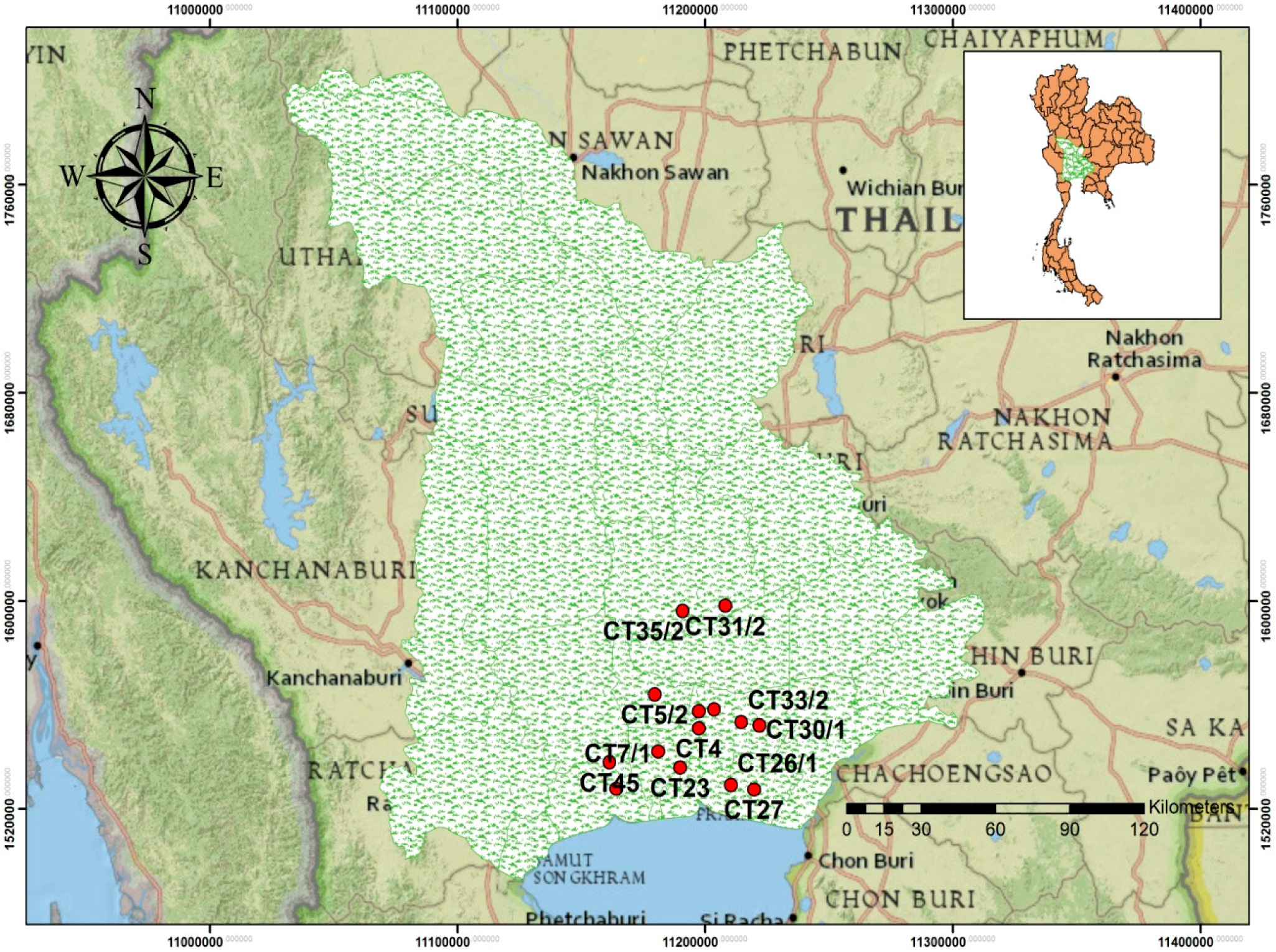
The groundwater basin in the lower Chao Phraya River is located in one of the most important and populous parts of Thailand, the lower central region. As shown in Figure 1, the area covers about 20 provinces with approximately 43,333 km2 and has the biggest groundwater basin in Thailand, at 269.312 billion m3. The area can be divided into 2 major parts. The lower plains part covers the area from the plain in Manorom city in Chainat province to the estuary area of the Chao Phraya River, which contains the water from the ground level to about 600 m deep. The other part is the borders of the Chao Phraya basin on both the east and west side, which is a mountainous area and has less water. The west side of the Chao Phraya basin edge covers the area from Uthai Thani province and the west side of Suphanburi province to Nakorn Pathom province. The east side of the Chao Phraya basin edge covers the area from Lopburi province, Saraburi province, Nakorn Nayok province, Prachinburi province and Cha Choeng Sao province.
Most of the area is the lower plains, except the north of Nakorn Pathom province, which is an upland area. The Chao Phraya River is the major river that runs from the north of Phra Nakorn Sri Ayutthaya province to the estuary area in Samut Prakarn province. The characteristics and types of rock and the geological structure of the edge of lower central region plain are mostly river sediment that flowed into the sediment basin, which is composed of Quaternary deposits. The hydrogeology of the lower central region plains is composed of both unconsolidated rocks and consolidated rocks [47].
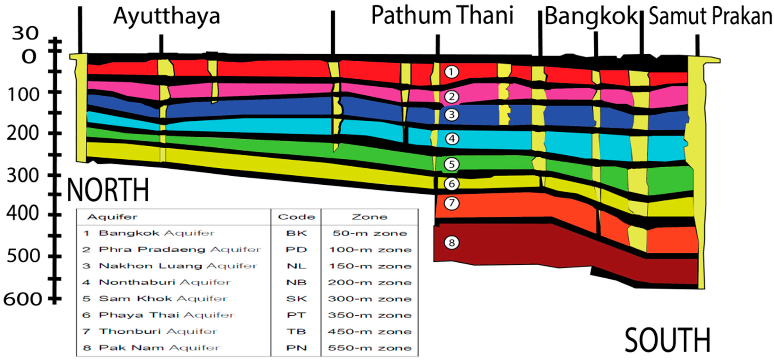
From the drill hole in the studied area, which collected data to a depth of 700 m, it was found that there is a groundwater level, which is the gravel level and which could be divided into 8 levels, as shown in Figure 2, which is modified from Asian Institute of Technology [48].
The water levels in wells that are screened in the upper-most unit (Bangkok aquifer) are going to respond differently from the water levels in wells in deeper hydrogeologic units. Because the upper-most unit wells have been influenced by the ground water recharge such as precipitation and stream runoff, the response happens more quickly than in other wells.
4. Methodology
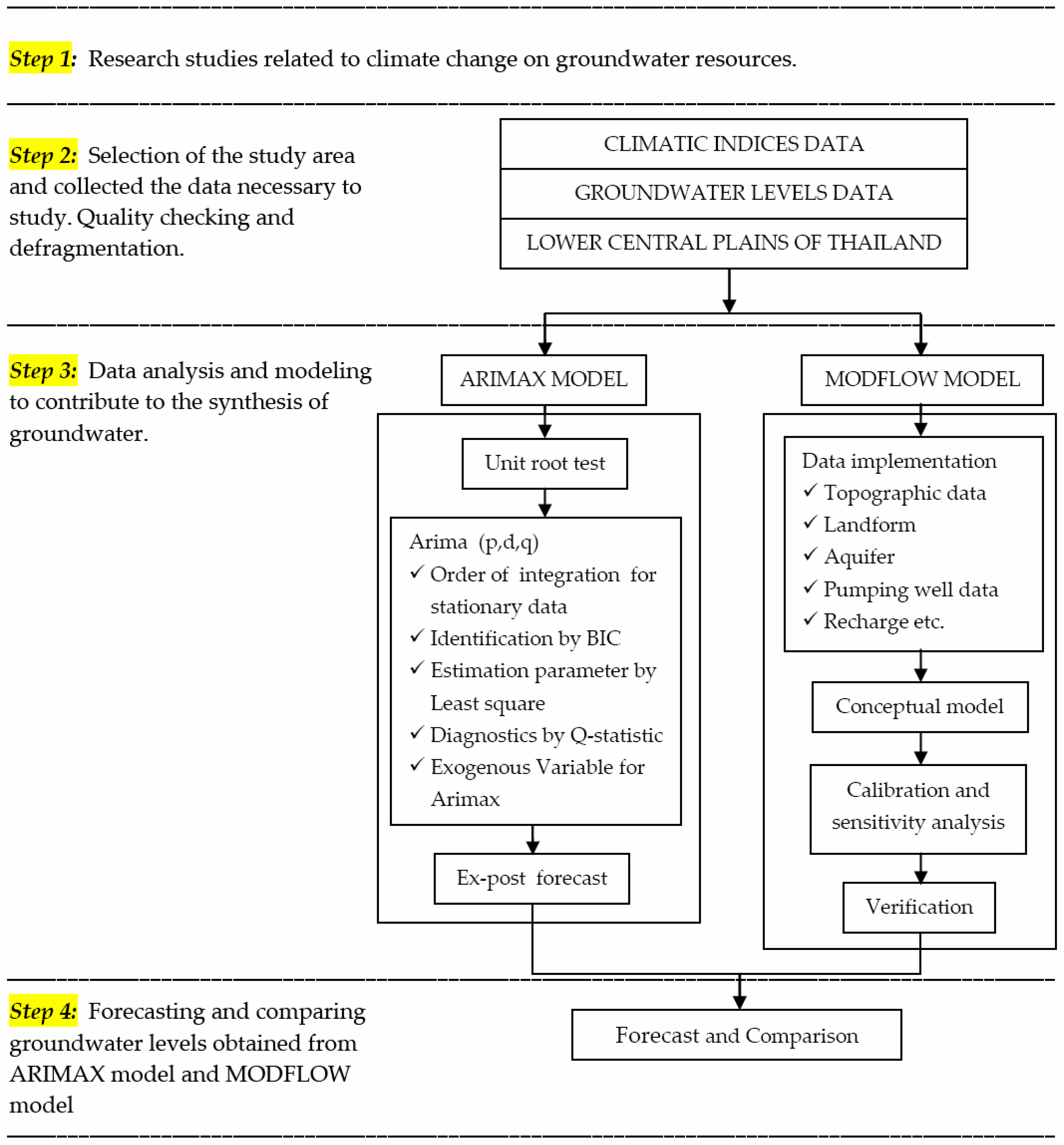
The data collected included a climatic/oceanography index and groundwater levels, to study the interrelation between them by analysis of ARIMAX. The water level forecasting of the ARIMAX method was compared with groundwater levels obtained from the simulation MODFLOW model, a flowchart of methodology shown in Figure 3 and the details are discussed below.
4.1. Available Data
4.1.1. Climatic Indices Data
According to NOAA, the major climate variation of this region is the Asian summer monsoon, which is analyzed with the Indian Summer Monsoon Index (IMI) and Western North Pacific Monsoon Index (WNPMI) and the Indian Ocean Dipole (IOD) is analyzed with the Dipole Mode Index. Those indices were used to consider the differences in sea water surface temperature around the equator area from the western Indian Ocean (50–70° E and 10° S–10° N) to the southeastern part of the Indian Ocean (90–110° E and 10° S–10° N).
Another phenomenon in this region is the El Nino–Southern Oscillation (ENSO), which involves several indices, such as the Multivariate ENSO Index (MEI), Southern Oscillation Index (SOI) and Sea Surface Temperature (SST). NINO4 is in the western equatorial part of the Pacific Ocean, or the so-called warm water basin and is located in latitude 5° N–5° S and longitude 150° W–160° E, which is the area that has the highest sea water temperature. It can affect many countries in the western Pacific; a total of 6 indices are used in analysis. The data also has been collected from 1960 to the present.
4.1.2. Groundwater Data
The monthly groundwater level data was monitored in wells in the lower Chao Phraya basin by the DGR. The data was collected from 14 wells in the studied area, which includes about 15 provinces; information from 4 sample stations is shown in Figure 4.
From the groundwater data that was collected from 1980 to 2012, measured from the land surface at the CT48-2 station, the water level has the highest variation and at the CT23 station, the water level has the lowest variation. At the same time, the average water level at the edge of the well is highest at CT33-2 station, at 47.60 m. The overall groundwater level has the negative kurtosis and negative skewness distribution.
4.2. Theory
When all necessary data, such as climate/oceanography index and groundwater level, had been collected, the model was developed using ARIMAX. It is one of the most popular statistical models in economic analytics for many types of time series forecasts, such as monthly incoming visitor forecasts [49] and daily car count forecasts [50]. ARIMAX has been constantly developed from the ARIMA mode, which had originally been presented by Box and Jenkins [51].
The climate/oceanography index+ and groundwater level used in the analysis should be stationary, so that the time series data has the constant mean (µ), variance (σ2) and covariance (γ). Therefore, the characteristics of the data need to be inspected with the unit root test, which can be done by using the Augmented Dicky-Fuller Test (ADF) [52] in 3 forms, as shown in Equations (1)–(3).
The parameter that is considered in every equation is δ. If δ = 0, Yt will have a unit root from comparing the calculated t-statistic value and the value from the Dickey-Fuller tables, or the MacKinnon critical values.
4.2.1. ARIMA Model
The Box-Jenkins method is the way to find the proper model for the time series value by using the Autocorrelation Function (ACF) and Partial Autocorrelation Function (PACF) to consider the model. The model is composed of 3 major parts, which are the Autoregressive Model (AR(p)), Integrated Process (I(d)) and Moving Average Model (MA(q)).
Autoregressive (AR(p)) is the model to show the observed yt value; it was assigned from the values of yt−1,...,yt−p or the previous observed value (p) by using the process of system AR(p), which is the process of the Autoregressive system at p order, which can be written as shown in Equation (4).
where yt is the groundwater level at time t; μ is the constant value; φi is the I ordered parameter; and εt is the error at time t.
Moving Average (MA(q)) is the model to calculate the observed yt value, which is assigned from the error at εt−1,…,εt−q or the previous error by using the process or system MA(q), which is the Moving Average at the q order, which can be written as in Equation (5).
The last step is to assign the proper model of the ARIMA model, which can be done by considering the Autocorrelation Function (ACF) and Partial Autocorrelation Function (PACF). In considering the Autoregressive Process model at p ordered and Moving Average at q ordered would result in Autoregressive Integrated Moving Average mode at p, d and q ordered, or ARIMA (p,d,q), which can be written as shown in Equation (6).
where yt is the groundwater level at time t; p is the order of Autoregressive; d is the number of times that differences were found in the constant characteristic time series data; q is the order of Moving Average; ∆d is the sign of finding the difference at d ordered (d-th difference operator); δ is the constant value; φ1, φp is the parameter of Autoregressive; θ1, θq is the parameter of Moving Average; εt is the error at the time t, which has been assigned to be white noise; and t is the time index.
4.2.2. ARIMAX Model
ARIMAX is the model that was adapted by including X, which is the leading variable (or Structural Variable or Exogenous Variable) to improve the forecasting accuracy. In this study, this variable is the climate and oceanography index and was newly formulated into Equation (6) to create Equation (7), as follows.
When the independent variable is included in the ARIMA model, it results in the ARIMAX model, shown in Equation (8).
where θ(L) is for Lag Polynomial, where .
In Equation (8), xt is the climate/oceanography index, where θ(L) is the degree of polynomial of the Exogenous variable that affects the Endogenous variable.
In testing to see whether X influences Y or not but using the null hypothesis (that is, H0: X does not influence Y) which can be said that to conclude that X influences Y, the null hypothesis needs to be rejected and when the variable passes the leading index testing, that variable could then be used to analyze the ARIMAX model.
When the proper order of ARIMAX model has been set up from the consideration of Bayesian Information Criteria (BIC), diagnostics should be done by the insignificant Ljung-Box Q statistic. After the most proper model is devised, then the groundwater level should be forecast to compare with the observed value, to compute the Root Mean Square Error (RMSE) and Mean Absolute Percent Error (MAPE). Finally, the groundwater level forecast by the statistical process would then be compared to the groundwater level that was synthesized from the physical model, which is MODFLOW in this case.
5. Conceptual Groundwater Model
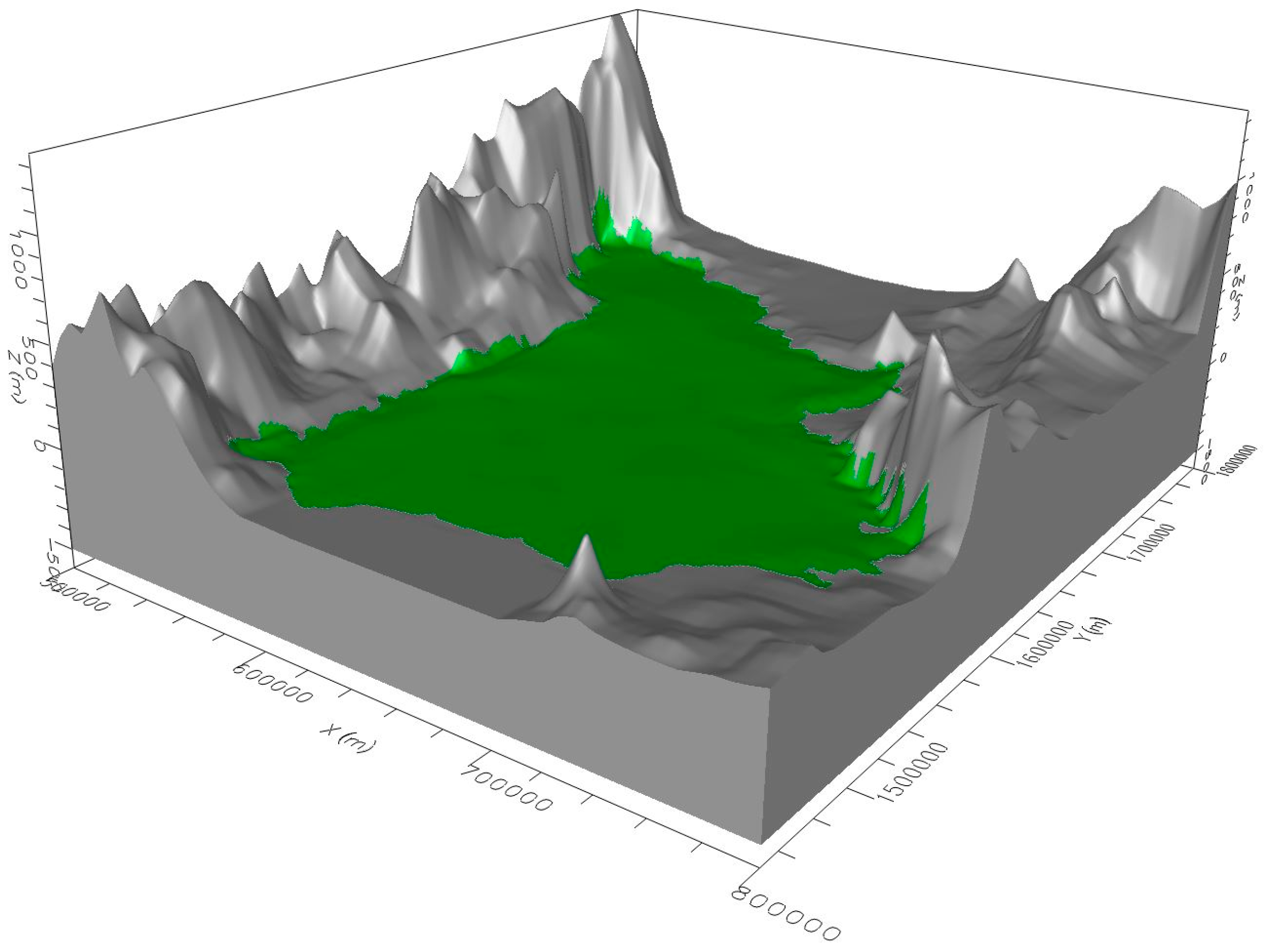
The analysis of data composed of geological data, hydrogeological data, groundwater characteristics, geographical data, groundwater usage data, mapping data and hydrological cross section graphics, which are partly modified from Arlai et al. [45], Department of Groundwater Resources [47] and Fornés and Pirarai [53], resulted in the conceptual model by MODFLOW as shown in Figure 5. The model is rectangular between (north-south) UTM 1,450,000 to 1,800,000 m and (east-west) 500,000 to 800,000 m. By having a fixed grid size at 1 km2, the model has a total of 945,000 grids, which are divided into 9 layers, comprising 8 layers of groundwater and the average 20-m thick Bangkok clay as the top layer.
5.1. Boundary
The hydrogeological model employs the following assumptions. The groundwater in the study area flows from north to south, which shows that horizontal permeability is better than vertical. The density of water is constant. Each aquifers layer is heterogeneous and anisotropic. The confining beds are homogeneous and isotropic. The groundwater flow is in steady state and the no-flux boundary around the area means that all aquifers are inactive cells, as shown in Figure 6, except for the south set, which is the constant head boundary. The water level at the Gulf of Thailand edge is set to be +0.00 m (MSL), according to Barlow [54] and Langevin [55], as shown in Table 1. The proper boundary of the model is in accordance with the hydrogeological characteristic of groundwater basin system in lower Chao Phraya from the study of DGR, such as the aquifer type of the Bangkok clay, on the top, which is set as an unconfined aquifer. But the groundwater from the Bangkok (BK) aquifer all the way to the Pak Nam (PN) aquifer is set as confined.
5.2. Parameters
The Digital Elevation Model (DEM) data is imported in order to have the height of the top and bottom of each layer as the model. The ground surface elevation is imported from the elevation data of the DGR national chart at the scale of 1:50,000. The study area has the elevation level at around 0–900 m above MSL. The initial head of every water layer is set from the groundwater level using the data from the wells observed by the DGR in 2009.
The assumption initially set the soil layer to be heterogeneous and anisotropic, referred from the hydraulic conductivity in the model by Spitz and Moreno [56]. The initial values for the calculation are shown in Table 2.
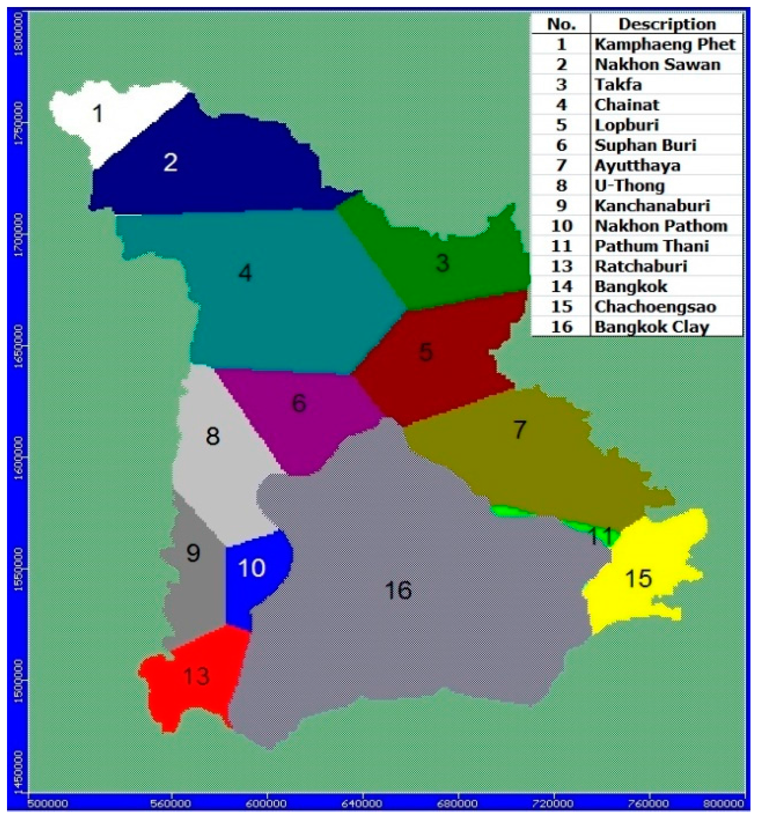
Estimation of the recharge rate is derived from the study by the DGR, which calculated the recharge rate to be about to 10% of rainfall in the area [57]. In this study, the rainfall distribution is set as Thiessen polygons, which are divided into 15 areas, as shown in Figure 7. Bangkok and the vicinity is found to be mostly the 20-m thick Bangkok clay. Therefore, there is no set recharge rate in this area.
The data of the major rivers in the study area–the Chao Phraya River, Tha Chin River, Pa Sak River and Mae Klong River–include river cross section graphic, river stage, riverbed bottom and the river width, from the Royal Irrigation Department. Bangkok and its vicinity are covered by the Bangkok clay, resulting in no recharging water from the river into the top layer of the model. However, the recharge from the river is still significant to the recharging area outside of Bangkok. The riverbed bottom level such Table 3 of the rivers is laid down on the second layer of the model (BK aquifer).
The pumping rate data is for groundwater users authorized by the DGR. The data is estimated by comparing the water usage rate in each province divided by the number of wells. Approximately 8800 wells are distributed over the area shown in Figure 8. Actually, there are still more users that use just a little water but they are not authorized; water smuggling also occurs but there is no data that could be included in this model development.
5.3. Simulation Scenarios
This study models in the steady state by initial calibration with data from 2009 to 2010, since, during this time, the data is quite complete and has little variation, corresponding to the steady flow hypothesis. To obtain a representative hydraulic conductivity value, the model was verified by using the period 2011–2012. The value of the recharge was adjusted every month, including 24 values into the model. The monthly groundwater level of each month was synthesized. Finally, the groundwater level is obtained and compared with the groundwater level forecast by the ARIMAX method.
6. Results and Discussion
6.1. Unit Root Test
The unit root test was done to consider whether the data is stationary [I(0); integrated of order 0] or nonstationary [I(d); d > 0; integrated of order d], to avoid the spurious regression or the timely nonstationary average and fluctuation data, by using the ADF (Augmented Dicky-Fuller Test) of the groundwater level data from 14 stations.
The initial time series data test found that the groundwater level data was nonstationary. The results from the ADF on values of each station showed that the values were lower than the critical value at the 0.01 and 0.05 significant level and under the null hypothesis acceptance (H0: θ = 0), which means that this data set had unit root. Then, the time series data was adjusted to be stationary by transforming the time series data with the 1st difference. When the adjusted data was retested with the ADF, the results showed that the ADF test statistic values were all higher than the critical value at the 0.01 and 0.05 significance level. This means that the 1st differential data were suitable for developing the ARIMA and ARIMAX model for forecasting the groundwater level in the study area, as shown in Table 4.
6.2. Identification
Initially, according to the principal of ARIMA modeling, considering the correlation graph of ACF and PACF of the groundwater level in each station, no station showed any sign of nonstationary seasonal form or data which was related to the unit root test result. The correlation graph of ACF showed the long-term regression, while in the correlation graph of PACF, the value quickly lowered to zero at every tested station. The sample of CT4 station in Figure 9 shows that the PACF lowered to 0 in lag 2.
After adjusting the time series data to be stationary by transforming the initial time series groundwater level data with the 1st difference, or ARIMA(p,1q) and after considering the correlogram of ACF and PACF, such as the time series, the results of the CT4 station are shown in Figure 10. It was found to be a stationary time series. Therefore, the forecasting model is possible, as shown in Table 5.
Table 6 shows the possible models of individual study stations, based on the correlogram of ACF and PACF. The model for station CT4 is probably only one form, ARIMA(0,1,2), while station CT5/2 has probably 2 models: ARIMA(1,1,10) and ARIMA(0,2,4). The model that has the lowest value of BIC is ARIMA(1,1,10), which would be used in forecasting for station CT5/2. The other stations are considered in the same way.
In Table 6, the constant term coefficient is −0.033. The t-statistic value is close to 0, with the 0.05 significance level. This means that the constant term relies on ∆yt. On the other hand, the coefficient of AR(4) is 0.169. The t-statistic value is 3.079, which is far from 0, with the significance level at 0.05. This means that the change of AR(4) is in the same direction with ∆yt. The coefficient of MA(1) is 0.891 and the t-statistic value is 18.618, which is different from 0, with the significance level at 0.05. This means that the change of MA(1) is in the same direction as ∆yt.
6.3. Parameter Estimation
6.4. Diagnostics
The results of diagnostic checking for white noise consideration of estimated residual (εt) show that the correlogram of residuals of autocorrelation (ACF) show no sign of exponential regression. At the same time, the calculated Box and Ljung (Q-statistic) value is lower that the critical value of Chi-square at the 0.10 significance level (prob. < 0.10), which means that εt is white noise or has normal distribution. The mean is equal to 0 and variances σ2, so it could be said that εt has no autocorrelation and no heteroscedasticity. Table 7 shows the analytic results, showing that all the time series samples passed the diagnostic checking and were suitable for use in forecasting.
6.5. ARIMAX
In the ARIMA model, more of the exogenous parameter would be included in the study, such as the climate/oceanology index, IMI, WNPMI, DMI, MEI, SOI and NINO4. All of these were brought in for the Granger Causality Test to see if the index could influence the groundwater level in the study area. The leading parameter test was at the 95% confidence level, so the leading parameter test result was different from station to station. The analytic results of the CT30/1 station are shown in Table 8.
Table 8 shows that the 1-month lag IMI index, 3-month lag MEI index, 3-month lag SOI index and 1-month lag WNPMI index were the leading parameters of the groundwater level. The DMI and Nino index were not the cause of groundwater level at the CT30/1 station, because the test rejected the hypothesis “H0: The test index was not the cause of groundwater level” and accepted the hypothesis “H0: The groundwater level was not the cause of the text index”. The test results of each station for the ARIMAX model are shown in Table 9.
The model from Table 9 can be used to make forecasts in the short time interval for the 14-station monthly groundwater level data in 2011. This was used for accuracy confirmation checking by using the Relative Root Mean Square Error (RRMSE) index. If the RRMSE value was more than 1, the ARIMAX forecasting had less error than the ARIMA model forecasting. Table 10 shows the comparison of RRMSE value between the ARIMAX model and the ARIMA model. At all stations, the forecasting results of ARIMAX model had obviously fewer errors than the ARIMA model, which means that including more climate indices in the ARIMAX model results in more accurate forecasting.
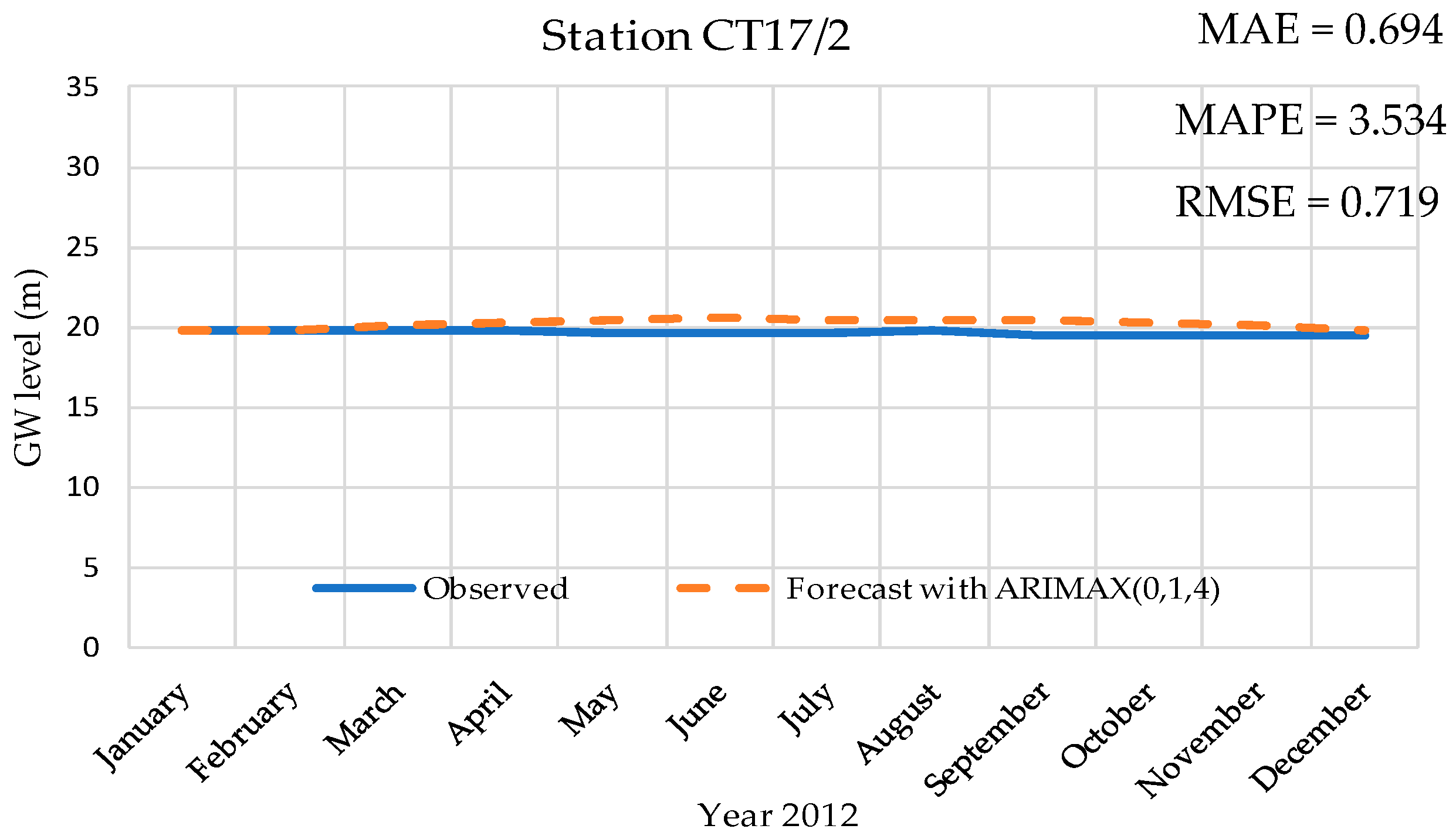
After the suitable ARIMAX model had been developed, it was used for the Ex-ante forecast because the ARIMAX model performed very well in the short time interval forecasting. In this study, 12 time intervals were selected for forecasting, January 2012 to December 2012. The forecast value then was compared with the real data. Figure 11 shows the sample of 12-month groundwater level forecasts for CT17/2 station. The forecast value was 19.75 in January 2012 and 19.87 in December 2012. The Root Mean Square Error (RMSE) was 0.719 and MAPE was 3.434% for this station. The results were used for Ex-ante forecasting to compare with the groundwater level data synthesized from the MODFLOW model in the same time interval as the step.
6.6. MODFLOW Simulation in Steady State
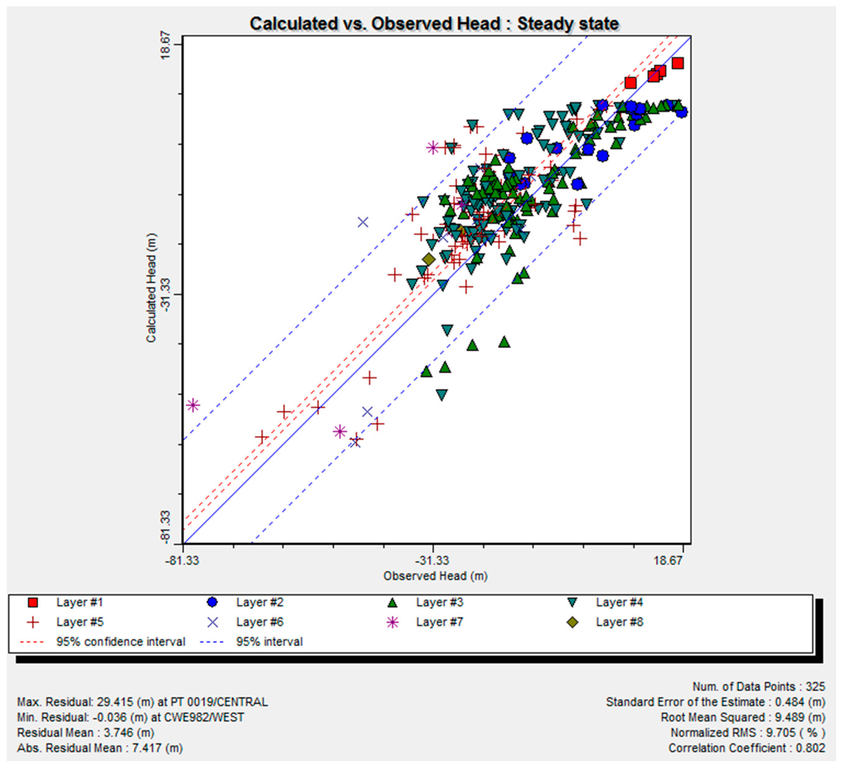
After the adjustment of the model using the 325 observed wells distributed in the study area, it was found that the calculated water pressure had the Absolute Residual Mean equal to 7.417 m; the Root Mean Squared Error (RMSE) was 9.489 m; the Normalized RMS was 9.705%; and the Correlation Coefficient was 0.802, as shown in Figure 12.
The water level from the model in the steady state has the error in the comparison of the calculated value and the real value measured from the observed wells because there is a large number of observed wells and the study area is vast. Moreover, the assigned hydraulic conductivity for each aquifer had to be the least possible, for the purpose of simplicity of the model. Each aquifer had been set with approximately 2 values–the calibrated vertical hydraulic conductivity and the calibrated horizontal hydraulic conductivity–as shown in Table 11.
Groundwater flow characteristics of the model assume flow from the edge of the area to the middle of the basin and from north to south. From the retrieved equipotential line and flow direction, the model related to the conceptual model, as shown in Figure 13.
From the verification of groundwater level at 325 wells, using the parameter adjustment of the model from the data in 2011, the water level at the time was quite steady, compared with the data from other years. The calculated water pressure value had the Absolute Residual Mean at 9.024 m; Root Mean Squared Error (RMSE) at 11.575 m; Normalized RMS at 11.54%; and Correlation Coefficient at 0.724. The error was seen to be a little higher than those of the calibration.
The sensitivity analysis of the model was carried out by repeating the modeling, by changing the parameters in the model one by one, after the completion of the model adjustment (which related to the conceptual model and had small error), to see the head pressure error caused by changes in each parameter. If any parameter caused a major change, this could mean that that parameter was pertinent to the change in the model.
Changing parameters one at a time and 25% at a time resulted in sensitivity analysis of the model and a better understanding of the influences of the parameters on the model. This information could be used to plan the additional field data collection, to adjust the model for differences in future hydrogeological conditions, or to make the fine parameter adjustments to have smaller errors and to confirm the parameter set correctness before continuing to the next step of model development. From the sensitivity analysis in Figure 14, looking at the relationship between the percentage of parameter changing and the absolute residual mean of head pressure, it was found that the most influential parameter changes were the hydraulic conductivity (K), the pumping rate and RCH value, in that order.
After the process of sensitivity analysis and changing parameters, the verification of the model was repeated with the monthly recharge value at approximately 10% of the monthly rainfall from 2012, in order to synthesize the monthly groundwater level in comparison with the groundwater level retrieved from the ARIMAX model.
6.7. Comparison of ARIMAX Groundwater Level and MODFLOW Groundwater Level
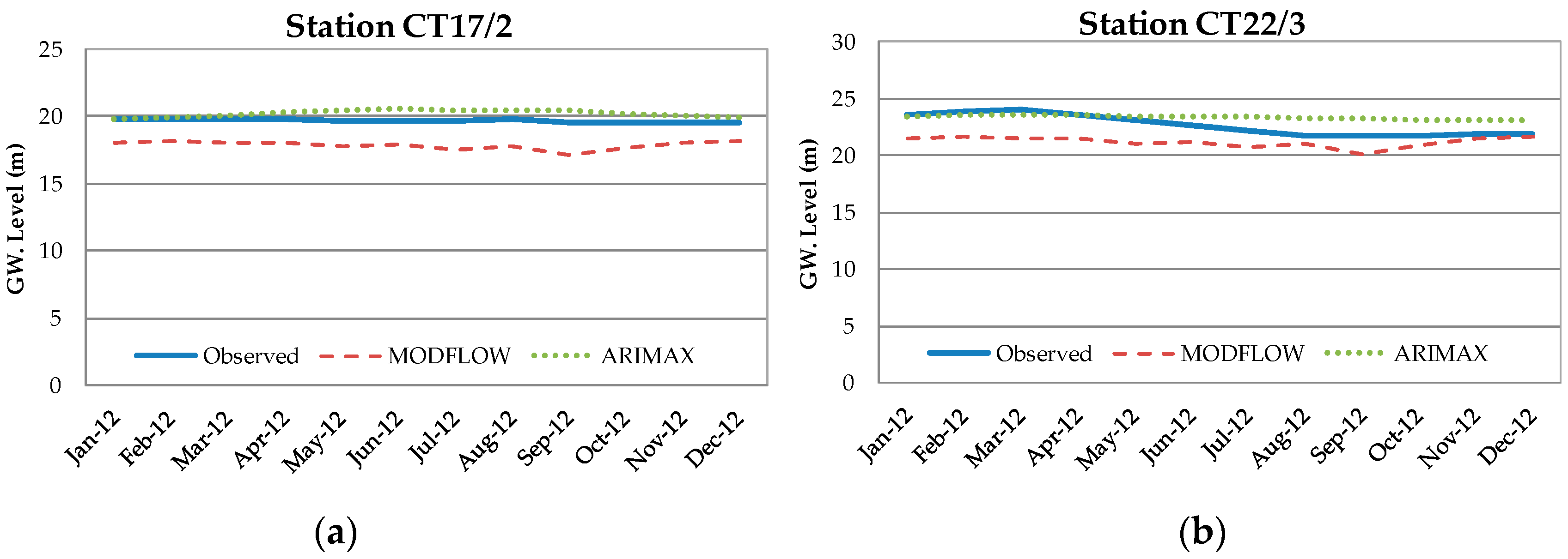
The forecast groundwater level from both ARIMAX and MODFLOW were compared by use of the Relative Root Mean Square Error (RRMSE). The results show that the ARIMAX model gave more accurate results than MODFLOW gave. Figure 15 shows the sample of the forecasting at CT17/2 and CT22/3 stations that were done by the MODFLOW model at the 95% confidence interval, which gave results close to the ARIMAX model. In some wells that were outside of the 95% confidence interval, more different forecast results would be presented. It could go up to 100% error in some wells. However, the MODFLOW model analysis in this case was set to be steady flow, so the data brought into the model needed to use the average value, which could have some error.
The advantage of using the ARIMAX analysis in this case is the ability to analyze the groundwater level for each well accurately by using only the past groundwater level data and climate indices that were suitable for the case. For MODFLOW, more physical data were needed, such as geographical data, aquifer and river water level, to develop the model. However, there were a number of advantages to using MODFLOW, such as the convenience in importing data about the complex aquifers, ease of data pre-processing and post-processing and the ability to display the regional results, which could clearly show the flow behavior. The selection depended on the analysis objective of each case.
7. Conclusions
Groundwater is affected both directly and indirectly by climate change. Because groundwater recharge varies with the filling process, groundwater is dependent on many factors, such as the size and type of recharge area and the water recharge rate. These effects can be observed by monitoring groundwater levels continuously over a long period. Long-term observations will enable us to plan and manage groundwater use effectively.
The study examined the relationship between the climate index and the groundwater level in the lower Chao Phraya basin by using the climate indices, DMI, IMI, MEI, NINO4, SOI and WNPMI and groundwater level data for 14 stations between 1980 and 2012. In the ARIMAX analysis, the first step was to analyze the stationary characteristics of data before finding the proper model by the Unit Root Test, using the Augmented Dicky-Fuller Test (ADF Test). The results show that the groundwater level was not steady; therefore, the time-series data transformation using the 1st difference was applied, in order to have more appropriate data. The ARIMA model consideration was done by considering the correlogram of ACF and PACF, which gave around 25 possible forms. The BIC statistics were then used to select 1 form per station. The next step was to perform the diagnostic checking to consider the white noise characteristics of the estimated residual (εt) by the Box and Ljung process (Q-statistic); in this step, it was found that every selected form was appropriate. The Granger Causality Test of the leading parameters and climate indices was applied to see which index could be used in the ARIMAX model and could forecast the groundwater level for 2012. The results showed that the groundwater level was related to the climate index and could give an effective forecast result at the approximate average RMSE of 0.6. The MODFLOW model then was developed for the study area, with 8 groundwater layers and topped with Bangkok clay. Other boundaries were set to be steady. The verification was done according to the procedure giving the monthly groundwater level result in 2012 at the 95% confidence interval, close to those from the ARIMAX modelling.
The time series forecast of groundwater level by ARIMAX found that it can predict better than ARIMA. It shows that the groundwater level is linked to the climate index and the use of exogenous variables is appropriate. The groundwater simulation model using Visual MODFLOW was found to have advantages in many applications. Importing complicated aquifer information is convenient and it is easy to perform pre-processing and post-processing. However, the definitions of the conditions in this model may not correspond to the actual state of nature, so the simulation results may differ slightly from observation data.
In this study, the MODFLOW model was used with the basic parameter boundary setting and the steady state analysis. The study could be further done in the transient condition. Although, the sensitivity analysis showed that the groundwater pumping was the important parameter, there are still a lot of other unpresented groundwater usage data. This lack of data is one of the cause resulted in the error of the model. If the groundwater pumping influence could be cut out of the groundwater level data [58], the model could then have more chance to get higher accuracy.
Climate change is expected to affect the groundwater resources and the world’s populations in the future, so it is going to be a genuine risk factor and will probably become increasingly severe. The study has shown that applying statistical analysis to the study and assessment of the relationship between the climate and the groundwater could be very useful for planning water use for sustainable development. A relatively small amount of data is required and the expense is not very high, either. This could be another way to cope with climate change effectively. In the past few decades, a lot more modeling techniques were presented to the research in hydrological modeling, such as, Artificial Neural Networks (ANNs) [59,60,61]. It would be more useful if these techniques were applied to the groundwater analysis.
Acknowledgments
For the successful completion of this research, the corresponding author would like to extend his deep gratitude to Uma Seeboonruang and the data was provided by the Bureau of Meteorology, as well as King Mongkut’s Institute of Technology Ladkrabang (KMITL). Authors acknowledge the support and cooperation of all these institutions. The authors are also sincerely grateful to the anonymous reviewers for providing thorough reviews and useful suggestions.
Author Contributions
Korrakoch Taweesin conducted the research, including data collection, analysis and preparation of the manuscript. Uma Seeboonruang and Phayom Saraphirom supervised the research, discussed the results and contributed to the finalization of the manuscript.
Conflicts of Interest
The authors declare no conflict of interest.
References
- Green, T.R.; Taniguchi, M.; Kooi, H.; Gurdak, J.J.; Allen, D.M.; Hiscock, K.M.; Treidel, H.; Aureli, A. Beneath the surface of global change: Impacts of climate change on groundwater. J. Hydrol. 2011, 405, 532–560. [Google Scholar] [CrossRef]
- Hanson, R.; Newhouse, M.; Dettinger, M. A methodology to asess relations between climatic variability and variations in hydrologic time series in the southwestern united states. J. Hydrol. 2004, 287, 252–269. [Google Scholar] [CrossRef]
- McBride, J.L.; Nicholls, N. Seasonal relationships between australian rainfall and the southern oscillation. Mon. Weather Rev. 1983, 111, 1998–2004. [Google Scholar] [CrossRef]
- Smithson, P.A. Ipcc, 2001: Climate change 2001: The scientific basis. Contrib. Work. Group 2002, 1, 1144. [Google Scholar]
- Morris, R.M.; Vergin, K.L.; Cho, J.-C.; Rappé, M.S.; Carlson, C.A.; Giovannoni, S.J. Temporal and spatial response of bacterioplankton lineages to annual convective overturn at the bermuda atlantic time-series study site. Limnol. Oceanogr. 2005, 50, 1687–1696. [Google Scholar] [CrossRef]
- UNEP Chemicals; Inter-Organization Programme for the Sound Management of Chemicals. Global Mercury Assessment; UNEP Chemicals: Nairobi, Kenya, 2002. [Google Scholar]
- Philander, S. E1 Nifio, La Nifia, and the Southern Oscillation; International Geophysics Series; Elsevier: Amsterdam, The Netherlands, 1990; Volume 46. [Google Scholar]
- Mantua, N.J.; Hare, S.R. The pacific decadal oscillation. J. Oceanogr. 2002, 58, 35–44. [Google Scholar] [CrossRef]
- Minobe, S. A 50–70 year climatic oscillation over the north pacific and North America. Geophys. Res. Lett. 1997, 24, 683–686. [Google Scholar] [CrossRef]
- Fye, F.K.; Stahle, D.W.; Cook, E.R.; Cleaveland, M.K. Nao influence on sub-decadal moisture variability over central North America. Geophys. Res. Lett. 2006, 33. [Google Scholar] [CrossRef]
- Kerr, R.A. A north Atlantic climate pacemaker for the centuries. Science 2000, 288, 1984–1985. [Google Scholar] [CrossRef] [PubMed]
- Chiew, F.H.; Piechota, T.C.; Dracup, J.A.; McMahon, T.A. El nino/southern oscillation and australian rainfall, streamflow and drought: Links and potential for forecasting. J. Hydrol. 1998, 204, 138–149. [Google Scholar] [CrossRef]
- Limjirakan, S.; Limsakul, A. Spatio-Temporal Changes in Total Annual Rainfall and the Annual Number of Rainy Days; International Atomic Energy Agency: Vienna, Austria, 2007. [Google Scholar]
- Kusreesakul, K. Spatio-Temporal Rainfall Changes in Thailand and Their Connection with Regional and Global Climate Variability. Master of Science Thesis, Environmental University, Prince of Songkla University, Hat Yai, Thailand, 2009. [Google Scholar]
- Limsakul, A.; Goes, J.I. Empirical evidence for interannual and longer period variability in thailand surface air temperatures. Atmos. Res. 2008, 87, 89–102. [Google Scholar] [CrossRef]
- Limsakul, A.; Limjirakan, S.; Suttamanuswong, B. Asian summer monsoon and its associated rainfall variability in thailand. Environ. Asia 2010, 3, 79–89. [Google Scholar]
- Kundzewicz, Z.W.; Mata, L.J.; Arnell, N.; Doll, P.; Kabat, P.; Jimenez, B.; Miller, K.; Oki, T.; Zekai, S.; Shiklomanov, I. Freshwater Resources and Their Management; Cambridge University Press: Cambridge, UK, 2007. [Google Scholar]
- Shah, T. Wells and Welfare in the Ganga Basin: Public Policy and Private Initiative in Eastern Uttar Pradesh, India; IWMI: Colombo, Sri Lanka, 2001; Volume 54. [Google Scholar]
- Pulido-Velazquez, D.; Garrote, L.; Andreu, J.; Martin-Carrasco, F.-J.; Iglesias, A. A methodology to diagnose the effect of climate change and to identify adaptive strategies to reduce its impacts in conjunctive-use systems at basin scale. J. Hydrol. 2011, 405, 110–122. [Google Scholar] [CrossRef]
- Taylor, R.G.; Scanlon, B.; Döll, P.; Rodell, M.; Van Beek, R.; Wada, Y.; Longuevergne, L.; Leblanc, M.; Famiglietti, J.S.; Edmunds, M. Ground water and climate change. Nat. Clim. Chang. 2013, 3, 322–329. [Google Scholar] [CrossRef] [Green Version]
- Holman, I.P. Climate change impacts on groundwater recharge-uncertainty, shortcomings, and the way forward? Hydrogeol. J. 2006, 14, 637–647. [Google Scholar] [CrossRef] [Green Version]
- Chen, Z.; Grasby, S.E.; Osadetz, K.G. Relation between climate variability and groundwater levels in the upper carbonate aquifer, southern manitoba, canada. J. Hydrol. 2004, 290, 43–62. [Google Scholar] [CrossRef]
- Hanson, R.; Dettinger, M.; Newhouse, M. Relations between climatic variability and hydrologic time series from four alluvial basins across the southwestern united states. Hydrogeol. J. 2006, 14, 1122–1146. [Google Scholar] [CrossRef]
- Faunt, C.C.; Hanson, R.; Belitz, K. Groundwater Availability of the Central Valley Aquifer, California; U.S. Geological Survey: Reston, VA, USA, 2009.
- Gurdak, J.J.; Hanson, R.T.; McMahon, P.B.; Bruce, B.W.; McCray, J.E.; Thyne, G.D.; Reedy, R.C. Climate variability controls on unsaturated water and chemical movement, high plains aquifer, usaall rights reserved. No part of this periodical may be reproduced or transmitted in any form or by any means, electronic or mechanical, including photocopying, recording, or any information storage and retrieval system, without permission in writing from the publisher. Vadose Zone J. 2007, 6, 533–547. [Google Scholar]
- Yusoff, I.; Hiscock, K.; Conway, D. Simulation of the impacts of climate change on groundwater resources in eastern england. Geol. Soc. Lond. Spec. Publ. 2002, 193, 325–344. [Google Scholar] [CrossRef]
- Loaiciga, H.; Maidment, D.; Valdes, J. Climate-change impacts in a regional karst aquifer, texas, USA. J. Hydrol. 2000, 227, 173–194. [Google Scholar] [CrossRef]
- Arnell, N.W. Climate change and water resources in britain. Clim. Chang. 1998, 39, 83–110. [Google Scholar] [CrossRef]
- Stringham, T.K.; Krueger, W.C.; Thomas, D.R. Application of non-equilibrium ecology to rangeland riparian zones. J. Range Manag. 2001, 210–217. [Google Scholar] [CrossRef]
- Chen, Z.; Grasby, S.E.; Osadetz, K.G. Predicting average annual groundwater levels from climatic variables: An empirical model. J. Hydrol. 2002, 260, 102–117. [Google Scholar] [CrossRef]
- Cooper, V.; Nguyen, V.; Nicell, J. Evaluation of global optimization methods for conceptual rainfall-runoff model calibration. Water Sci. Technol. 1997, 36, 53–60. [Google Scholar]
- Croley, T.E.; Luukkonen, C.L. Potential effects of climate change on ground water in lansing, michigan. J. Am. Water Resour. Assoc. 2003, 39, 149–163. [Google Scholar] [CrossRef]
- Rios, M.A.; Kirschen, D.S.; Jayaweera, D.; Nedic, D.P.; Allan, R.N. Value of security: Modeling time-dependent phenomena and weather conditions. IEEE Trans. Power Syst. 2002, 17, 543–548. [Google Scholar] [CrossRef]
- Changnon, S.A.; Huff, F.A.; Hsu, C.-F. Relations between precipitation and shallow groundwater in illinois. J. Clim. 1988, 1, 1239–1250. [Google Scholar] [CrossRef]
- Adhikary, S.K.; Rahman, M.; Gupta, A.D. A stochastic modelling technique for predicting groundwater table fluctuations with time series analysis. Int. J. Appl. Sci. Eng. Res. 2012, 1, 238–249. [Google Scholar]
- Ahn, H.; Salas, J.D. Groundwater head sampling based on stochastic analysis. Water Resour. Res. 1997, 33, 2769–2780. [Google Scholar] [CrossRef]
- Ahn, H. Modeling of groundwater heads based on second-order difference time series models. J. Hydrol. 2000, 234, 82–94. [Google Scholar] [CrossRef]
- Mirzavand, M.; Ghazavi, R. A stochastic modelling technique for groundwater level forecasting in an arid environment using time series methods. Water Resour. Manag. 2015, 29, 1315–1328. [Google Scholar] [CrossRef]
- Harbaugh, A.W.; Banta, E.R.; Hill, M.C.; McDonald, M.G. Modflow-2000, the U.S. Geological Survey Modular Ground-Water Model-User Guide to Modularization Concepts and the Ground-Water Flow Process; Open-File Report; U.S. Geological Survey: Reston, VA, USA, 2000; p. 134.
- Lawrence, A.; Barker, J.; Boonyakarnkul, T.; Chanvaivit, S.; Nagesuwan, P.; Sirirat, P.; Stuart, M.; Thandat, P.; Varathan, P. Impact of Urbanisation on Groundwater: Hat Yai. Thailand; British Geological Survey (BGS): Keyworth, UK, 1994. [Google Scholar]
- Margane, A. Environmental Geology for Regional Planning; Department of Mineral Resources: Bangkok, Thailand, 2001.
- Department of Groundwater Resources. Experrimental Study on the Addition of Water to Groundwater through the Pond System in the Northern Water Shed Area (Pisanulok, Sukhothai and Pichit); Ministry of Natural Resources and Environment: Putrajaya, Malaysia, 2011.
- Fogg, G.E. Groundwater flow and sand body interconnectedness in a thick, multiple-aquifer system. Water Resour. Res. 1986, 22, 679–694. [Google Scholar] [CrossRef]
- Maxwell, R.M.; Kollet, S.J. Interdependence of groundwater dynamics and land-energy feedbacks under climate change. Nat. Geosci. 2008, 1, 665–669. [Google Scholar] [CrossRef]
- Arlai, P.; Koch, M.; Koontanakulvong, S. Statistical and stochastic approaches to assess reasonable calibrated parameters in a complex multi-aquifer system. In Proceedings of the “CMWR XVI-Computational Methods in Water Resources, Copenhagen, Denmark, 19–22 June 2006. [Google Scholar]
- Voss, C.I. Editor’s message: Groundwater modeling fantasies—Part 1, adrift in the details. Hydrogeol. J. 2011, 19, 1281–1284. [Google Scholar] [CrossRef]
- Department of Groundwater Resources. Study on the Impact of Underground Structure Due to the Restoration of Water Pressure in Bangkok and Vicinity; Ministry of Natural Resources and Environment: Bangkok, Thailand, 2012.
- Asian Institute of Technology. Sustainable Water Management Policy (SWMP) Study on Groundwater Management Bangkok, Thailand; Asian Institute of Technology: Bangkok, Thailand, 2007. [Google Scholar]
- Lim, C.; Min, J.C.; McAleer, M. Modelling income effects on long and short haul international travel from japan. Tour. Manag. 2008, 29, 1099–1109. [Google Scholar] [CrossRef]
- Williams, B. Multivariate vehicular traffic flow prediction: Evaluation of arimax modeling. Transp. Res. Rec. J. Transp. Res. Board 2001, 194–200. [Google Scholar] [CrossRef]
- Box, G.E.; Jenkins, G.M. Time Series Analysis: Forecasting and Control; Holden-Day: San Francisco, CA, USA, 1976. [Google Scholar]
- Dickey, D.A.; Fuller, W.A. Distribution of the estimators for autoregressive time series with a unit root. J. Am. Stat. Assoc. 1979, 74, 427–431. [Google Scholar]
- Fornés, J.; Pirarai, K. Groundwater in thailand. J. Environ. Sci. Eng. B 2014, 3, 304–315. [Google Scholar]
- Barlow, P.M. Ground Water in Fresh Water-Salt Water Environments of the Atlantic; Geological Survey (USGS): Reston, VA, USA, 2003; Volume 1262.
- Langevin, C.D. Simulation of Ground-Water Discharge to Biscayne Bay, Southeastern Florida; U.S. Geological Survey: Reston, VA, USA, 2001.
- Spitz, K.; Moreno, J. A Practical Guide to Groundwater and Solute Transport Modeling; John Wiley and Sons: Hoboken, NJ, USA, 1996. [Google Scholar]
- Sanford, W.E.; Buapeng, S. Assessment of a groundwater flow model of the bangkok basin, thailand, using carbon-14-based ages and paleohydrology. Hydrogeol. J. 1996, 4, 26–40. [Google Scholar] [CrossRef]
- Seeboonruang, U. An empirical decomposition of deep groundwater time series and possible link to climate variability. Global NEST J. 2014, 16, 87–103. [Google Scholar]
- Taormina, R.; Chau, K.-W.; Sivakumar, B. Neural network river forecasting through baseflow separation and binary-coded swarm optimization. J. Hydrol. 2015, 529, 1788–1797. [Google Scholar] [CrossRef]
- Chen, X.; Chau, K.; Busari, A. A comparative study of population-based optimization algorithms for downstream river flow forecasting by a hybrid neural network model. Eng. Appl. Artif. Intell. 2015, 46, 258–268. [Google Scholar] [CrossRef]
- Gholami, V.; Chau, K.; Fadaee, F.; Torkaman, J.; Ghaffari, A. Modeling of groundwater level fluctuations using dendrochronology in alluvial aquifers. J. Hydrol. 2015, 529, 1060–1069. [Google Scholar] [CrossRef]
Figure 1.
Location of study area and observations wells in the lower central plains of Thailand.

Figure 2.
The groundwater and aquifer levels in the study area.

Figure 3.
Methodological process for obtaining groundwater levels.

Figure 4.
Characteristics of groundwater levels at 4 sample stations.
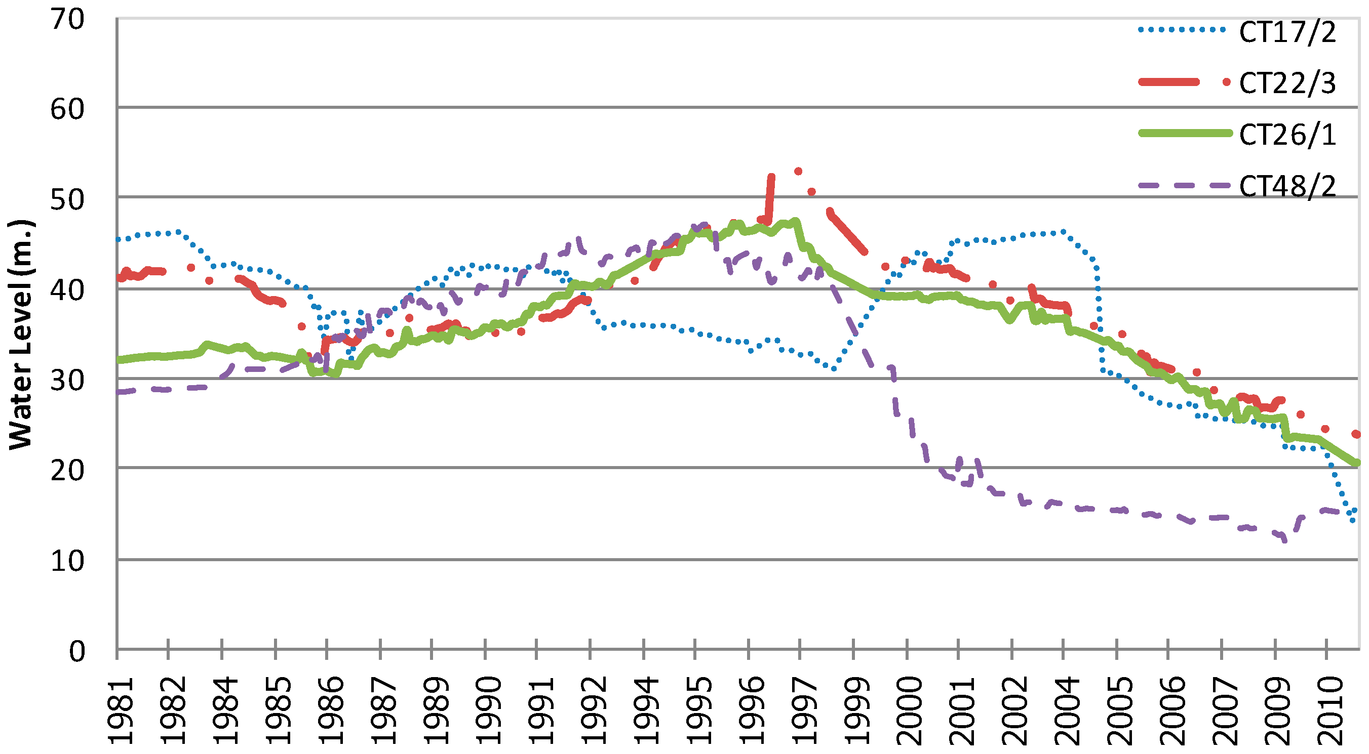
Figure 5.
The 3D boundary and conceptual model of study area.

Figure 6.
Study area and the no-flux boundary.
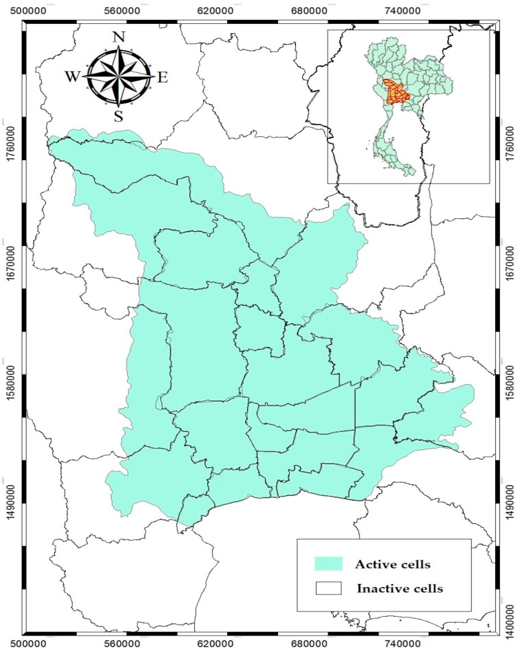
Figure 7.
The recharge area using the Thiessen polygon rainfall distribution in the study area.

Figure 8.
Distribution of pumping wells in the model.
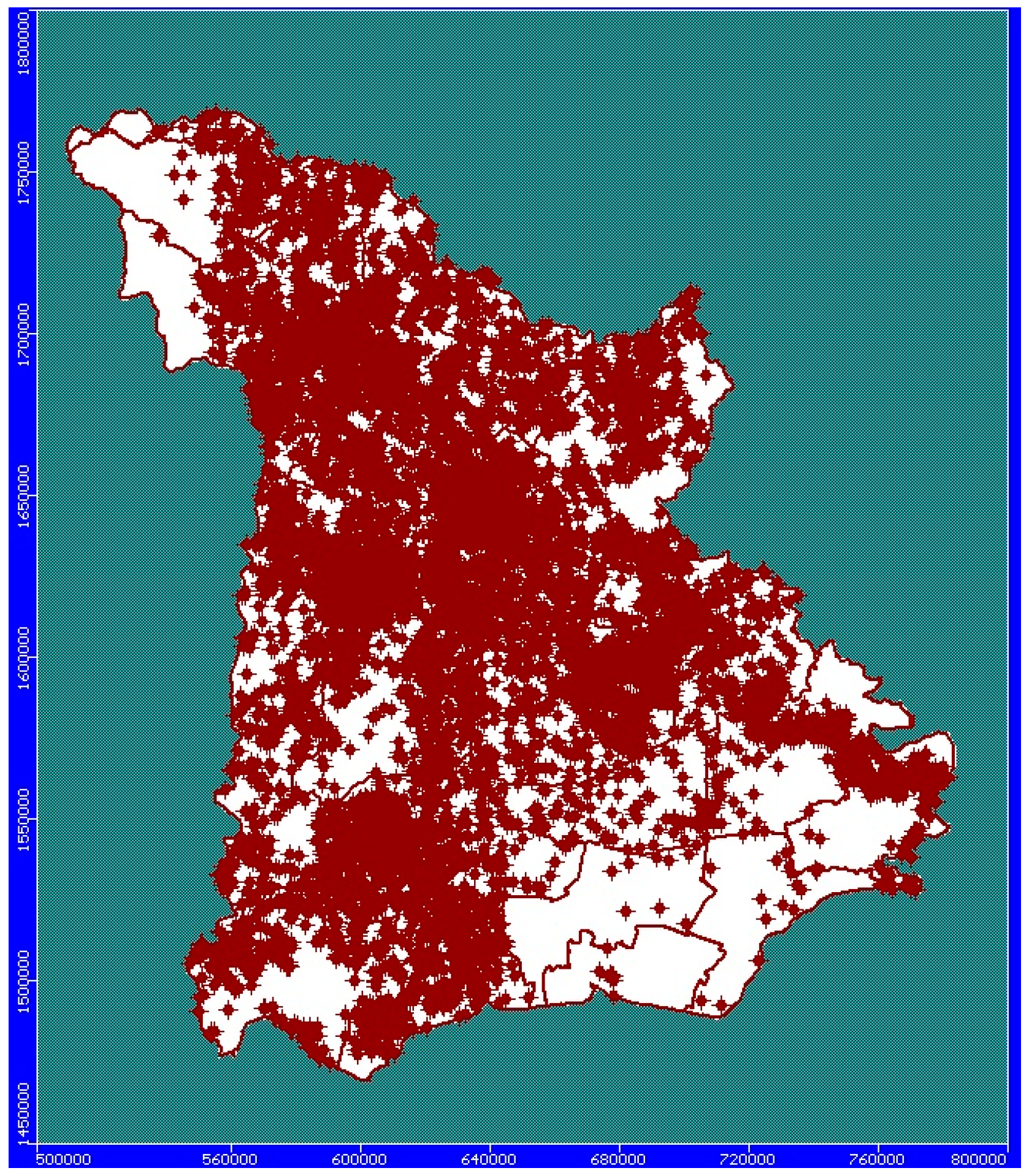
Figure 9.
Correlogram of ACF and PACF in case of ARIMA(0,0,0) analysis of CT4 station.
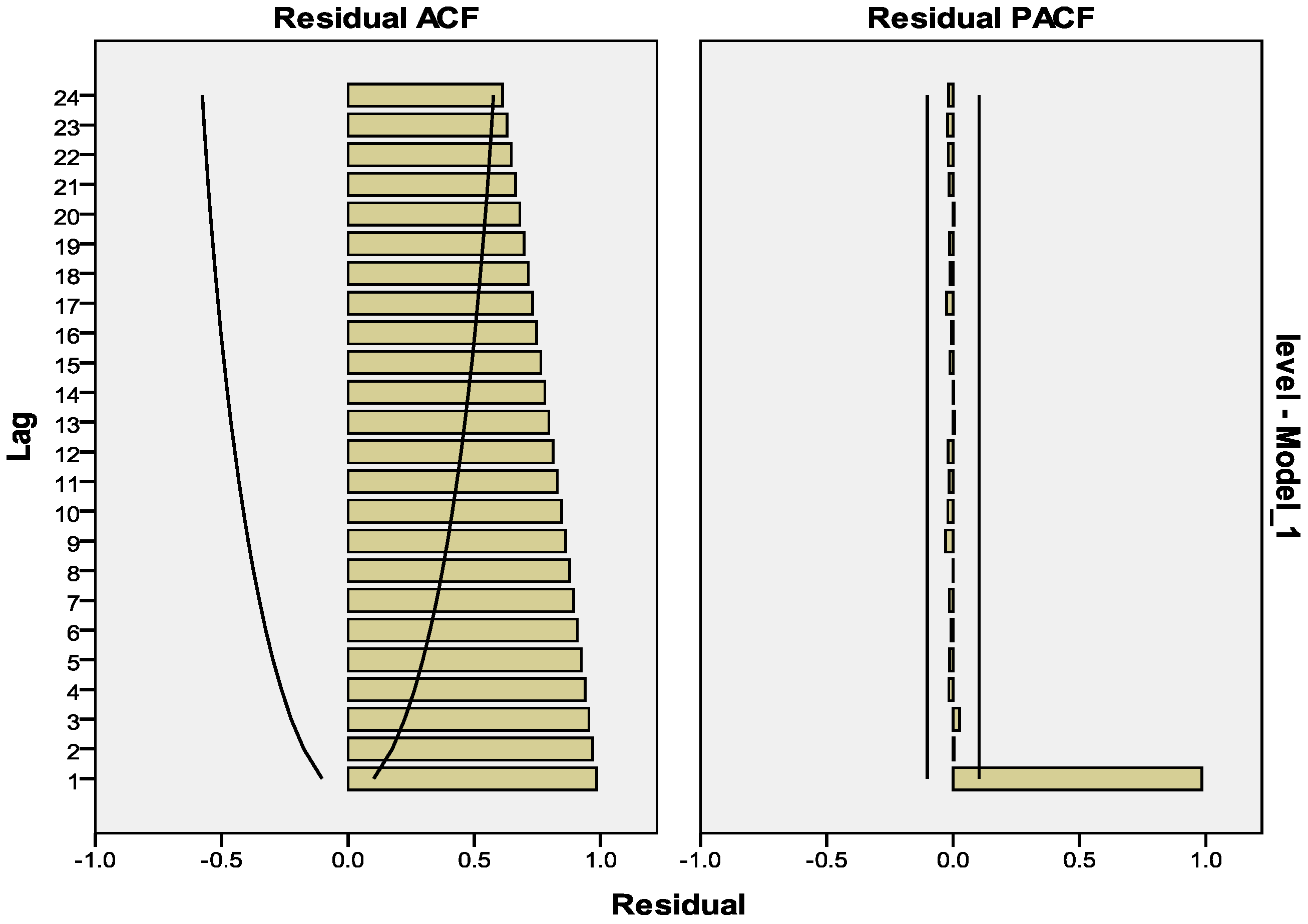
Figure 10.
Correlogram of ACF and PACF in the ARIMA(0,1,0) analysis of CT4 station.
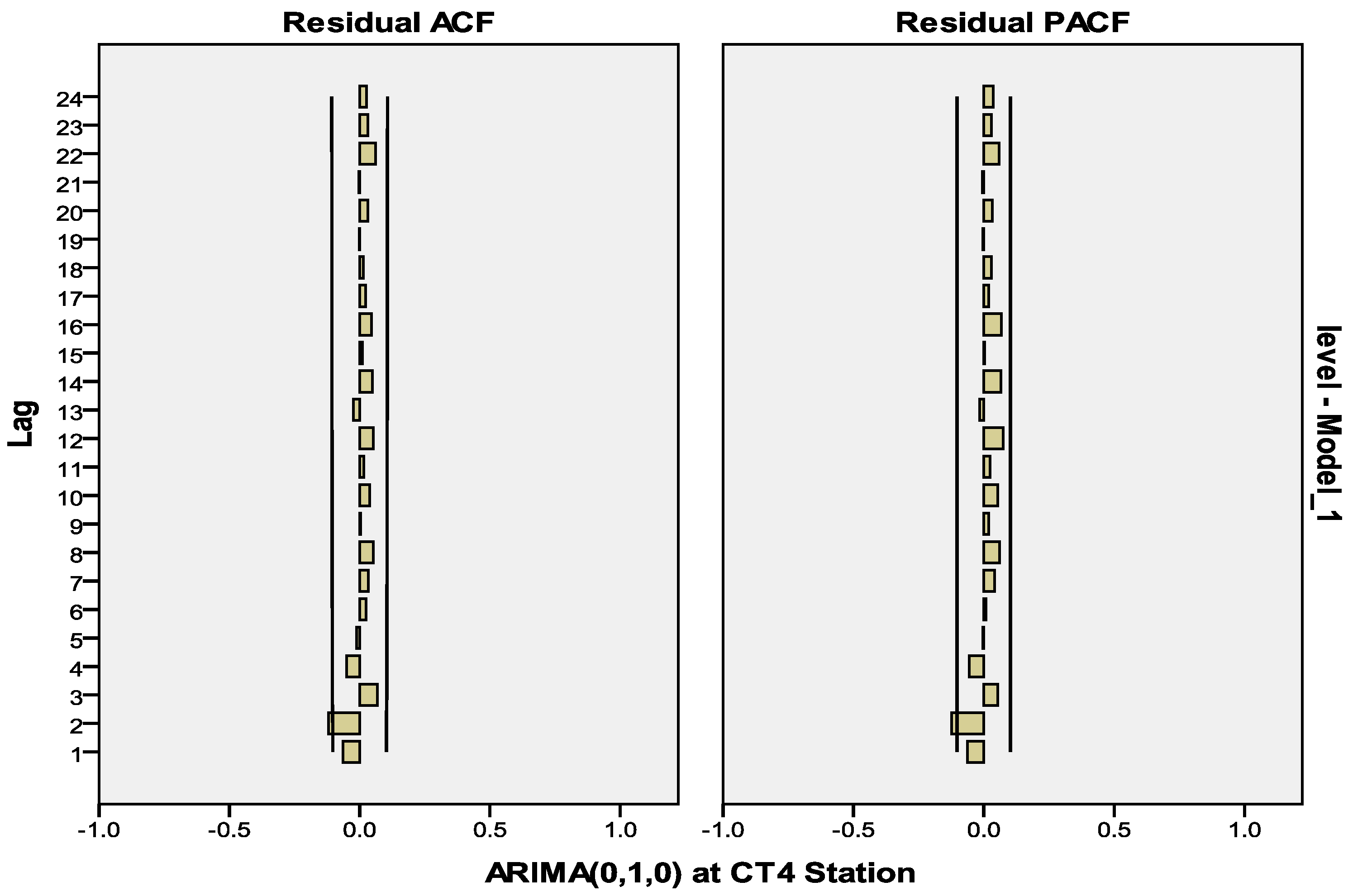
Figure 11.
Comparison of groundwater level in the Ex-ante forecast by the ARIMAX(0,1,4) model for the CT17/2 station.
Figure 11.
Comparison of groundwater level in the Ex-ante forecast by the ARIMAX(0,1,4) model for the CT17/2 station.

Figure 12.
Calibrated results of the groundwater level model in the study area.

Figure 13.
Equipotential line and flow direction results in the steady state: (a) Layer 1; (b) Layer 2.
Figure 13.
Equipotential line and flow direction results in the steady state: (a) Layer 1; (b) Layer 2.
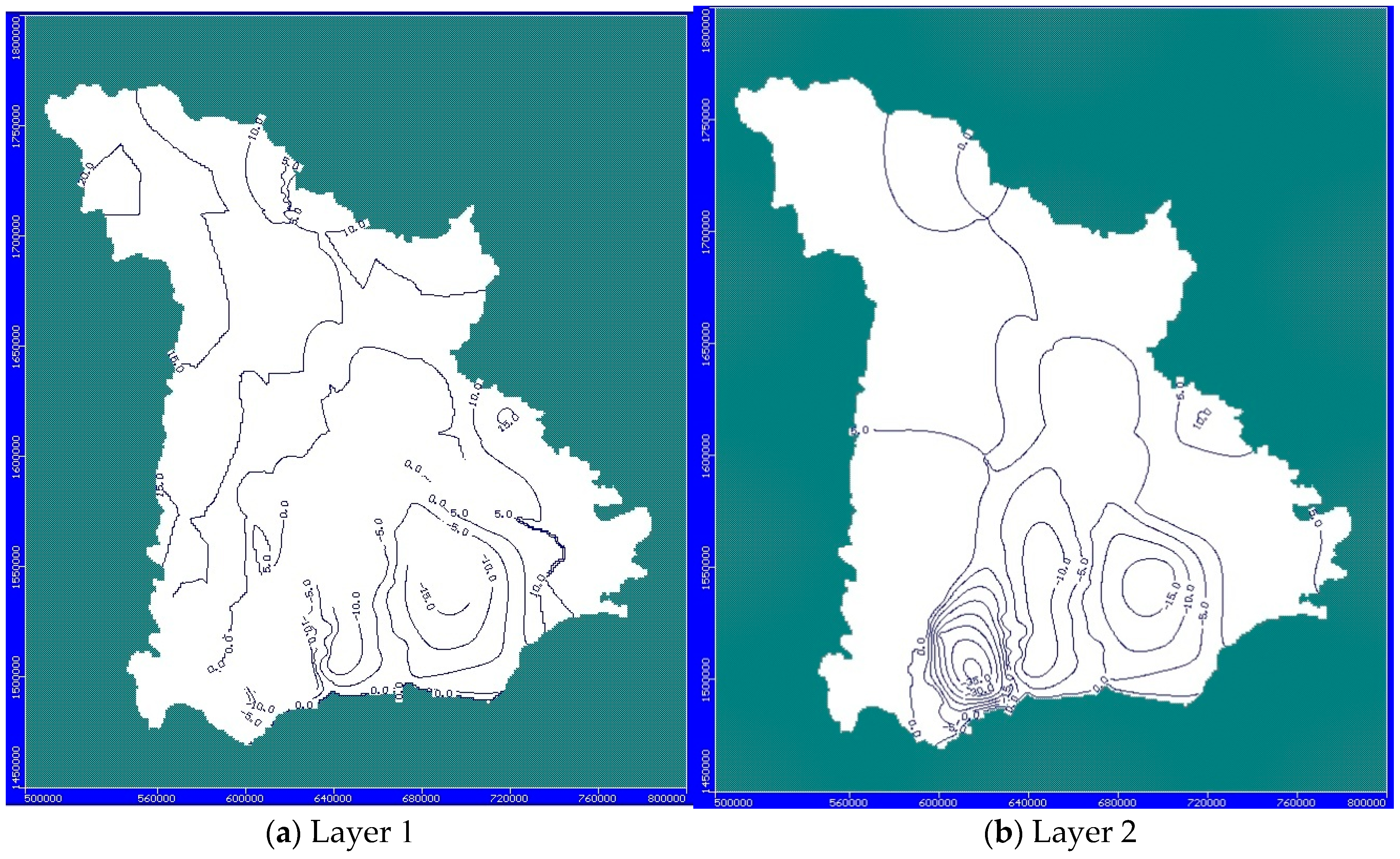
Figure 14.
Sensitivity analysis of the parameters in the MODFLOW model.
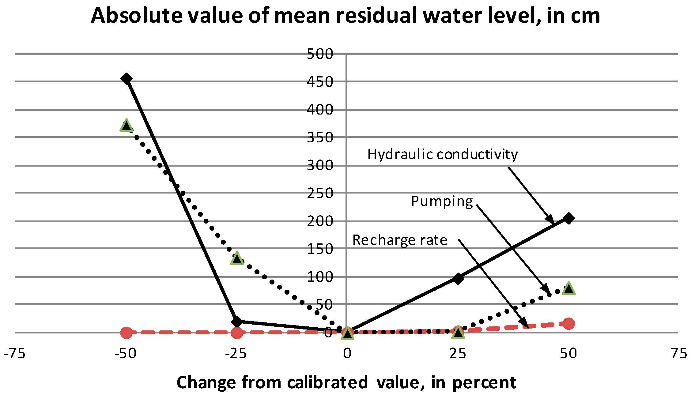
Figure 15.
Comparison of forecast groundwater levels between ARIMAX and MODFLOW, examples for (a) CT17/2 and (b) CT22/3 stations.
Figure 15.
Comparison of forecast groundwater levels between ARIMAX and MODFLOW, examples for (a) CT17/2 and (b) CT22/3 stations.


Table 1.
Mean hydraulic heads of the aquifers.
| Top to the Deepest | Aquifers | hf (m) |
|---|---|---|
| 1 | Bangkok (BK) | 1.00 |
| 2 | Phra Pradaeng (PD) | 2.25 |
| 3 | Nakorn Luang (NL) | 4.0 |
| 4 | Nonthaburi (NB) | 6.25 |
| 5 | Sam Khok (SK) | 7.5 |
| 6 | Phaya Thai (PT) | 8.75 |
| 7 | Thonburi (TB) | 11.25 |
| 8 | Pak Nam (PN) | 13.75 |
Table 2.
Initial hydraulic conductivity, K, for model.
| Zone | Kx (m/s) | Ky (m/s) | Kz (m/s) |
|---|---|---|---|
| 1 | 3.50 × 10⁻⁹ | 3.50 × 10⁻⁹ | 3.50 × 10⁻¹⁰ |
| 2 | 1.50 × 10⁻² | 1.50 × 10⁻² | 1.50 × 10⁻³ |
| 3 | 9.50 × 10⁻⁷ | 9.50 × 10⁻⁷ | 9.50 × 10⁻⁸ |
| 4 | 9.00 × 10⁻⁵ | 9.00 × 10⁻⁵ | 9.00 × 10⁻⁶ |
| 5 | 3.50 × 10⁻⁶ | 3.50 × 10⁻⁶ | 3.50 × 10⁻⁷ |
| 6 | 3.00 × 10⁻⁷ | 3.00 × 10⁻⁷ | 3.00 × 10⁻⁸ |
| 7 | 8.50 × 10⁻⁸ | 8.50 × 10⁻⁸ | 8.50 × 10⁻⁹ |
| 8 | 1.50 × 10⁻⁶ | 1.50 × 10⁻⁶ | 1.50 × 10⁻⁷ |
| 9 | 3.00 × 10⁻⁹ | 3.00 × 10⁻⁹ | 3.00 × 10⁻¹⁰ |
| 10 | 8.00 × 10⁻⁵ | 8.00 × 10⁻⁵ | 8.00 × 10⁻⁶ |
| 11 | 2.00 × 10⁻¹⁰ | 2.00 × 10⁻¹⁰ | 2.00 × 10⁻¹¹ |
| 12 | 1.00 × 10⁻⁶ | 1.00 × 10⁻⁶ | 1.00 × 10⁻⁷ |
| 13 | 8.00 × 10⁻⁴ | 8.00 × 10⁻⁴ | 8.00 × 10⁻⁵ |
| 14 | 8.00 × 10⁻⁸ | 8.00 × 10⁻⁸ | 8.00 × 10⁻⁹ |
| 15 | 6.30 × 10⁻⁴ | 6.30 × 10⁻⁴ | 6.30 × 10⁻⁵ |
| 16 | 5.70 × 10⁻⁶ | 5.70 × 10⁻⁶ | 5.70 × 10⁻⁷ |
| 17 | 1.00 × 10⁻⁹ | 1.00 × 10⁻⁹ | 1.00 × 10⁻¹⁰ |
Table 3.
Values of the river boundary parameter for the RIV of the initial model.
| River | River Stage (m. msl.) | Riverbed Bottom (m. msl.) |
|---|---|---|
| Mae Klong River | 2.274–(−5.785) | 0.311–(−6.625) |
| Tha Chin River | (−0.289)–(−2.694) | (−2.828)–(−4.328) |
| Chao Phraya River | (−3.252)–(−2.928) | (−9.673)–(−12.075) |
| Pa Sak River | 11.486–(−2.417) | 7.606–(−12.698) |
Table 4.
Results of the unit root test.
| Station | Level | First Difference | ||||
|---|---|---|---|---|---|---|
| ADF | MacKinnon Critical | ADF | MacKinnon Critical | |||
| 1% | 5% | 1% | 5% | |||
| CT4 | −0.603 | −3.983 | −3.422 | −20.590 | −3.983 | −3.422 |
| CT5/2 | 1.713 | −3.983 | −3.422 | −14.080 | −3.983 | −3.422 |
| CT7/1 | 0.013 | −3.983 | −3.422 | −14.156 | −3.983 | −3.422 |
| CT17/2 | −1.301 | −3.983 | −3.422 | −15.747 | −3.983 | −3.422 |
| CT22/3 | −0.101 | −3.983 | −3.422 | −11.451 | −3.983 | −3.422 |
| CT23 | −0.761 | −3.983 | −3.422 | −22.690 | −3.983 | −3.422 |
| CT26/1 | 0.230 | −3.983 | −3.422 | −19.002 | −3.983 | −3.422 |
| CT27 | 0.916 | −3.983 | −3.422 | −19.491 | −3.983 | −3.422 |
| CT30/1 | −0.639 | −3.983 | −3.422 | −13.330 | −3.983 | −3.422 |
| CT31/2 | −2.816 | −3.983 | −3.422 | −6.091 | −3.984 | −3.422 |
| CT33/2 | 0.143 | −3.983 | −3.422 | −22.445 | −3.983 | −3.422 |
| CT35/2 | 1.225 | −3.983 | −3.422 | −16.313 | −3.983 | −3.422 |
| CT45 | −0.342 | −3.983 | −3.422 | −21.881 | −3.983 | −3.422 |
| CT48/2 | −1.663 | −3.983 | −3.422 | −21.548 | −3.983 | −3.422 |
Table 5.
Possible model of each station.
| Observation Wells | Seasonal | Model | BIC | Proper Model |
|---|---|---|---|---|
| CT4 | None | ARIMA(0,1,2) | −2.358 | ARIMA(0,1,2) |
| CT5/2 | None | ARIMA(1,1,10) | −0.974 | ARIMA(1,1,10) |
| None | ARIMA(0,2,4) | −0.997 | ||
| CT7/1 | None | ARIMA(0,1,3) | −2.09 | ARIMA(0,1,4) |
| None | ARIMA(0,1,4) | −2.086 | ||
| CT17/2 | None | ARIMA(1,1,0) | −0.485 | ARIMA(0,1,4) |
| None | ARIMA(0,1,4) | −0.468 | ||
| CT22/3 | None | ARIMA(2,1,0) | −1.291 | ARIMA(2,1,0) |
| None | ARIMA(1,1,1) | −1.303 | ||
| CT23 | None | ARIMA(0,1,1) | −1.732 | ARIMA(0,1,1) |
| CT26/1 | None | ARIMA(4,1,0) | −1.812 | ARIMA(4,1,0) |
| None | ARIMA(1,1,1) | −1.89 | ||
| CT27 | None | ARIMA(4,1,0) | −2.845 | ARIMA(4,1,0) |
| None | ARIMA(1,1,1) | −2.899 | ||
| CT30/1 | None | ARIMA(2,1,0) | −2.334 | ARIMA(2,1,0) |
| None | ARIMA(0,1,2) | −2.337 | ||
| CT31/2 | None | ARIMA(0,1,0) | −1.744 | ARIMA(0,1,0) |
| CT33/2 | None | ARIMA(1,1,2) | −0.38 | ARIMA(1,1,2) |
| None | ARIMA(2,1,1) | −0.381 | ||
| CT35/2 | None | ARIMA(13,1,0) | −2.893 | ARIMA(13,1,0) |
| None | ARIMA(0,1,13) | −2.9 | ||
| CT45 | None | ARIMA(1,1,6) | −0.783 | ARIMA(1,1,6) |
| None | ARIMA(1,2,2) | −0.847 | ||
| CT48/2 | None | ARIMA(1,2,4) | −0.57 | ARIMA(4,1,1) |
| None | ARIMA(4,1,1) | −0.577 |
Table 6.
Parameter estimation of ARIMA(4,1,1) model of CT48/2 station.
| Variable | Coefficient | Std. Error | t-Statistic | Prob. |
|---|---|---|---|---|
| Constant | −0.033 | 0.102 | −0.326 | 0.745 |
| AR(4) | 0.169 | 0.055 | 3.079 | 0.002 |
| MA(1) | 0.891 | 0.048 | 18.618 | 0.000 |
| R-squared | 0.996 | Ljung-Box Q | ||
| BIC | −0.570 | 18.634 | 0.135 | |
Table 7.
Diagnostic checking of selected models.
| Station | Model | Ljung-Box Q | Prob. |
|---|---|---|---|
| CT4 | ARIMA(0,1,2) | 12.369 | 0.718 |
| CT5/2 | ARIMA(1,1,10) | 25.831 | 0.072 |
| CT7/1 | ARIMA(0,1,4) | 29.503 | 0.109 |
| CT17/2 | ARIMA(0,1,4) | 10.213 | 0.746 |
| CT22/3 | ARIMA(2,1,0) | 22.271 | 0.135 |
| CT23 | ARIMA(0,1,1) | 7.976 | 0.967 |
| CT26/1 | ARIMA(4,1,0) | 26.044 | 0.126 |
| CT27 | ARIMA(4,1,0) | 25.131 | 0.083 |
| CT30/1 | ARIMA(2,1,0) | 12.025 | 0.742 |
| CT31/2 | ARIMA(0,1,0) | 11.225 | 0.885 |
| CT33/2 | ARIMA(1,1,2) | 14.047 | 0.522 |
| CT35/2 | ARIMA(13,1,0) | 10.337 | 0.066 |
| CT45 | ARIMA(1,1,6) | 12.591 | 0.321 |
| CT48/2 | ARIMA(1,2,4) | 17.876 | 0.162 |
Table 8.
Granger Causality Test of the groundwater level leading parameter at the CT30/1 station.
| Index | Lag (Months) | p-Value of H0 : | p-Value of H0 : | ||
|---|---|---|---|---|---|
| Index | GW Level | ||||
| Has No Granger Causality | Has No Granger Causality | ||||
| GW Level | Index | ||||
| DMI | - | - | - | - | - |
| IMI | 1 | 0.0319 | Reject | 0.6674 | Accept |
| MEI | 3 | 0.0342 | Reject | 0.9747 | Accept |
| NINO4 | - | - | - | - | - |
| SOI | 3 | 0.0145 | Reject | 0.8931 | Accept |
| WNPMI | 1 | 0.0318 | Reject | 0.9254 | Accept |
Table 9.
ARIMAX model of each station.
| Station | Model | BIC | Ljung-Box Q | ||
|---|---|---|---|---|---|
| CT4 | ∆y | constant | MA(2) DMI(-3) IMI(-2) NINO4(-3) | −2.307 | 9.172 |
| CT5/2 | ∆y | constant | AR(1) MA(10) DMI(-3) IMI(-3) MEI(-3) WNPMI(-2) | −0.900 | 7.407 |
| CT7/1 | ∆y | constant | MA(4) DMI(-1) SOI(-1) | −2.053 | 18.051 |
| CT17/2 | ∆y | constant | MA(4) MEI(-1) NINO4(-2) SOI(-1) | −0.437 | 7.840 |
| CT22/3 | ∆y | constant | AR(2) DMI(-1) IMI(-1) MEI(-1) | −1.241 | 20.781 |
| CT23 | ∆y | constant | MA(1) IMI(-2) SOI(-10) WNPMI(-2) | −1.672 | 6.874 |
| CT26/1 | ∆y | constant | AR(4) DMI(-3) IMI(-1) | −1.788 | 21.647 |
| CT27 | ∆y | constant | AR(4) IMI(-3) MEI(-3) SOI(-2) WNPMI(-2) | −2.780 | 18.694 |
| CT30/1 | ∆y | constant | AR(2) IMI(-1) MEI(-3) SOI(-3) WNPMI(-1) | −2.290 | 14.131 |
| CT31/2 | ∆y | constant | NINO4(-2) SOI(-2) | −1.720 | 11.206 |
| CT33/2 | ∆y | constant | AR(1) MA(2) IMI(-1) WNPMI(-3) | −0.376 | 15.899 |
| CT35/2 | ∆y | constant | AR(13) IMI(-1) SOI(-1) WNPMI(-4) | −2.893 | 7.994 |
| CT45 | ∆y | constant | AR(1) MA(6) DMI(-7) IMI(-4) WNPMI(-5) | −0.732 | 13.977 |
| CT48/2 | ∆y | constant | AR(4) MA(1) IMI(-5) MEI(-1) NINO4(-4) SOI(-1) | −0.513 | 16.629 |
Table 10.
Comparison of accuracy of ARIMA model and ARIMAX model forecasting.
| Station | Model | (1) | (2) | (3) = (1)/(2) |
|---|---|---|---|---|
| RMSE | RMSE | RRMSE | ||
| (ARIMA) | (ARIMAX) | – | ||
| CT4 | ARIMA(0,1,2) | 0.357 | 0.130 | 2.746 |
| CT5/2 | ARIMA(1,1,10) | 0.223 | 0.159 | 1.404 |
| CT7/1 | ARIMA(0,1,4) | 0.646 | 0.439 | 1.472 |
| CT17/2 | ARIMA(0,1,4) | 0.717 | 0.645 | 1.111 |
| CT22/3 | ARIMA(2,1,0) | 0.167 | 0.152 | 1.097 |
| CT23 | ARIMA(0,1,1) | 0.398 | 0.118 | 3.386 |
| CT26/1 | ARIMA(4,1,0) | 0.077 | 0.075 | 1.023 |
| CT27 | ARIMA(1,1,1) | 0.304 | 0.128 | 2.373 |
| CT30/1 | ARIMA(2,1,0) | 0.481 | 0.108 | 4.469 |
| CT31/2 | ARIMA(0,1,0) | 0.809 | 0.450 | 1.800 |
| CT33/2 | ARIMA(2,1,1) | 1.239 | 0.330 | 3.754 |
| CT35/2 | ARIMA(13,1,0) | 0.229 | 0.027 | 8.463 |
| CT45 | ARIMA(1,1,6) | 0.420 | 0.098 | 4.307 |
| CT48/2 | ARIMA(4,1,1) | 0.514 | 0.123 | 4.178 |
Table 11.
Hydraulic conductivity summary from the calibration in steady state.
| Layer | Kx [m/s] | Ky [m/s] | Kz [m/s] |
|---|---|---|---|
| 1 | 5.5 × 10 −9 | 5.5 × 10 −9 | 5.5 × 10 −10 |
| 2 | 0.00968 | 0.00968 | 0.000968 |
| 3 | 0.0099 | 0.0099 | 0.0099 |
| 4 | 0.0001 | 0.0001 | 1 × 10 −6 |
| 5 | 2.26 × 10 −6 | 2.26 × 10 −6 | 2.26 × 10 −7 |
| 6 | 2.23 × 10 −7 | 2.23 × 10 −7 | 2.23 × 10 −8 |
| 7 | 1.07 × 10 −7 | 1.07 × 10 −7 | 1.07 × 10 −9 |
| 8 | 2.76 × 10 −6 | 2.76 × 10 −6 | 2.76 × 10 −7 |
| 9 | 4.38 × 10 −10 | 4.38 × 10 −10 | 4.38 × 10 −11 |
| 10 | 4 × 10 −9 | 4 × 10 −9 | 4 × 10 −10 |
| 11 | 4.85 × 10 −5 | 4.85 × 10 −5 | 4.85 × 10 −7 |
| 12 | 9.48 × 10 −6 | 9.48 × 10 −6 | 9.48 × 10 −10 |
| 13 | 7.5 × 10 −8 | 7.5 × 10 −8 | 7.5 × 10 −9 |
| 14 | 8 × 10 −6 | 8 × 10 −6 | 8 × 10 −8 |
| 15 | 4.8 × 10 −8 | 4.8 × 10 −8 | 4.8 × 10 −9 |
| 16 | 9.1 × 10 −9 | 9.1 × 10 −9 | 9.1 × 10 −9 |
| 17 | 8.92 × 10 −7 | 8.92 × 10 −7 | 8.92 × 10 −8 |
© 2018 by the authors. Licensee MDPI, Basel, Switzerland. This article is an open access article distributed under the terms and conditions of the Creative Commons Attribution (CC BY) license (http://creativecommons.org/licenses/by/4.0/).
Share and Cite
MDPI and ACS Style
Taweesin, K.; Seeboonruang, U.; Saraphirom, P. The Influence of Climate Variability Effects on Groundwater Time Series in the Lower Central Plains of Thailand. Water 2018, 10, 290. https://doi.org/10.3390/w10030290
AMA Style
Taweesin K, Seeboonruang U, Saraphirom P. The Influence of Climate Variability Effects on Groundwater Time Series in the Lower Central Plains of Thailand. Water. 2018; 10(3):290. https://doi.org/10.3390/w10030290
Chicago/Turabian StyleTaweesin, Korrakoch, Uma Seeboonruang, and Phayom Saraphirom. 2018. "The Influence of Climate Variability Effects on Groundwater Time Series in the Lower Central Plains of Thailand" Water 10, no. 3: 290. https://doi.org/10.3390/w10030290
Note that from the first issue of 2016, this journal uses article numbers instead of page numbers. See further details here.