Evaluating Consistency between the Remotely Sensed Soil Moisture and the Hydrological Model-Simulated Soil Moisture in the Qujiang Catchment of China

Abstract

Accurate soil moisture estimation plays a crucial role in agricultural management and hydrological studies. Considering the scarcity of direct in-situ measurements, it is important to evaluate the consistency of soil moisture data acquired in indirect ways, including both satellite products and simulation values obtained via hydrological models. In this study, two types of high spatial-resolution remotely sensed values, namely the surface soil moisture (SSM) and the profile soil water index (SWI), are estimated from each of the ASCAT-A, ASCAT-B, SMAP and SMOS microwave satellites. They are compared with two groups of model-simulated daily soil moisture values, which are obtained by implementing the lumped Xinanjiang (XAJ) model and the DEM-based distributed hydrological model (DDRM) across the Qujiang catchment, located in southwest China. The results indicate that for each satellite product, SWI values always show closer agreement with model-simulated soil moisture values than SSM values, and SWI values estimated from ASCAT products perform best in terms of correlation coefficient with the model-simulated soil moisture, at around 0.8 on average, followed by the SMAP product, which shows a correlation coefficient of 0.48 on average, but the SMOS product shows poor performance. This evaluation of consistency provides useful information on their systematic differences and suggests subsequent studies to ensure their reconciliation in long-term records.

1. Introduction

As a key component in the hydrological cycle, soil moisture plays a crucial role in atmosphere-land surface interactions through controlling the available energy exchange among the hydrosphere, the atmosphere and the biosphere [1]. Thus, continuous and accurate acquisition of soil moisture data at local, regional and global scales is of vital importance for simulation of the climate system and the Earth system. However, current ways to obtain soil moisture fail to satisfy all these needs.

Soil moisture information can be obtained in both direct and indirect ways. The direct field measurements of soil moisture are thought to be fairly accurate, but are costly, with small coverage areas, and only provide point-based measurements rather than areal values, which are of more interest for practical applications. Indirect acquisition ways, including remote sensing (optical, thermal infrared and microwave) and hydrological models (either the physically-based land-surface models, or rainfall-runoff hydrological models), offer the possibility to provide the areal soil moisture information on a low-cost basis, but with less accuracy than ground point measurements [2,3].

Remote sensing (optical, thermal infrared and microwave) techniques can generally measure near-surface soil moisture contents [4]. The remotely sensed soil moisture of both optical and thermal techniques is thought to be vulnerable to easy contamination by weather conditions and many other noise sources, and their precision can hardly satisfy the needs of practical applications. In contrast, numerous studies have shown that microwave (passive and active) remotely sensed soil moisture has good potential for applications in different fields [5]. Active microwave satellites, include the Advanced Scatterometer (ASCAT) on the Meteorological Operational Satellite (Metop), emit a microwave signal and then acquire the backscatter signal strength reflected by the surface soil to retrieve soil moisture information [6,7]. These satellites provide soil saturation degrees ranging between zero (dry) to one (wet) with high spatial resolution but low temporal repeat. The mean values of these products are around 0.5. Passive microwave satellites, including the Advanced Microwave Scanning Radiometer for Earth Observing System (AMSR-E) and the Microwave Imaging Radiometer with Aperture Synthesis (MIRAS) on the Soil Moisture and Ocean Salinity (SMOS) satellite [8], receive natural microwaves from the Earth and then retrieve soil moisture through analyzing the dielectric properties of soil surfaces. These satellites provide soil moisture contents (m³ m⁻³) ranging between 0 and 0.6 with high temporal repeat but low spatial resolution. The mean values of these products are around 0.3. In addition, the National Aeronautics and Space Administration’s (NASA) Soil Moisture Active Passive (SMAP) mission, launched in 2015, aimed to retrieve soil moisture information from both active and passive microwave sensors [9]. All these microwave sensors can only acquire near-surface soil moisture content. Researchers have tried to combine different remotely sensed soil moisture products or proposed machine learning methods for better surface soil moisture estimations in recent years [10,11].

Soil moisture simulated by hydrological models is to represent the moisture contents at different layers or the total depth of the soil profile. Physically-based land-surface models, such as the Community Land Model (CLM) and the Variable Infiltration Capacity (VIC) models, account for both water and energy budgets to simulate multiple layers of surface soil moisture with complex parametrization schemes [12,13]. Rainfall-runoff hydrological models, which mainly account for only water budgets, can be further classified into lumped or distributed models, depending on their degree of spatial discretization of the catchment area. Lumped hydrological models provide catchment-averaged soil moisture contents of one or more upper layers of the soil profile, while the distributed models can provide the spatial distribution of the vertically-integrated or layered soil moisture information. For conceptual rainfall-runoff models, their soil moisture calculations vary in complexity with different simplifications and assumptions about the hydrological processes [14]. For example, the Xinanjiang (XAJ) model can simulate water storages in the upper, lower and deepest layer of the soil profile respectively [15]. TOPMODEL can simulate soil water storages at both the root-zone layer and the underlying unsaturated layer [16]. The DEM-based distributed model (DDRM) estimates the total soil moisture storage for the whole soil profile [17].

There have been some studies comparing microwave satellite soil moisture products with ground measurements or with both the model-simulated soil moisture and ground measurements at coarse spatial scales such as the catchment or sub-catchment scales [18,19,20,21,22] or at fine spatial scales such as grid scales [23,24]. For example, Reichle et al. compared the monthly Scanning Multichannel Microwave Radiometer (SMMR) soil moisture retrievals with the monthly soil moisture simulated by the NASA Catchment Land Surface Model for the period of 1979–1987 to examine their consistency, and validated these soil moisture values through the ground-based measurements [25]. Brocca et al. validated the reliability of the daily ASCAT soil moisture product through the comparisons with both the in-situ ground observations and the soil moisture simulated by a lumped hydrological (soil water balance) model but considered no comparisons between the model-simulated soil moisture and the ground measurements [26]. Albergel et al. used remotely sensed soil moisture to analyze soil moisture in a numerical weather prediction system in Europe, and evaluated both of them using global ground-based in situ observations from more than 200 stations located in Africa, Australia, Europe and the United States [27]. Al-Yaari et al. applied regression analysis on SMAP L-band temperature brightness observations by calibrating the regressions against SMOS soil moisture to obtain a new soil moisture dataset, and validated both of SMOS and SMAP soil moisture against in-situ measurements spread over the globe [28]. Pan et al. assessed SMAP soil moisture retrievals using high-resolution model simulations and in-situ observations [24]. Overall, in-situ soil moisture measurements are thought to be more accurate, and are more likely to be involved in comparing soil moisture information from different sources. However, comparing satellite soil moisture products and the model-simulated soil moisture with the ground measurements is in fact a challenging task for two reasons. One reason is that the in-situ ground measurements are not widely and easily available. Another reason is that they are usually point-based measurements and are sensitive to the small-scale land surface related components [29], compared to the satellite-based and the model-simulated soil moistures that are more sensitive to the atmospheric-forcing variability.

In areas where in-situ soil moisture measurements are sparse or hardly available, the satellite soil moisture products and the hydrological model-simulated soil moisture are two alternative sources of the soil moisture information. Remotely sensed soil moisture data have been integrated with models for different purposes. For example, calibrating hydrological models against remotely sensed soil moisture has attracted a lot of attention in hydrology in the last decade. Parajka et al. compared the European Remote-sensing Satellite (ERS) scatterometer soil moisture product with soil moisture simulations from a semi-distributed dual layer hydrological model for different seasons and elevations in Austria, and assessed the added value of satellite soil moisture estimates in the multiple objective calibration of the model [29]. Wanders et al. used remotely sensed soil moisture in parameter identification of large-scale lumped hydrological models to better simulate soil moisture content throughout the catchment and better simulate discharge in upstream areas. Besides, remotely sensed soil moisture products have also been used for updating the soil moisture states of models [13]. Grillakis et al. estimated antecedent soil moisture by remotely sensed soil moisture to contribute to the understanding of the importance of the initial soil moisture state for flash flood magnitudes simulated by a distributed model [30]. Alvarez-Garreton et al. improved streamflow prediction of a lumped hydrological model in data-scarce catchments by dual assimilation of remotely sensed soil moisture [31]. Tian et al. improved water balance component estimates of a distributed water balance model through joint assimilation of different remotely sensed soil moisture [32]. Once consistency between remotely sensed and hydrological model-simulated soil moisture is well evaluated, better potential will be offered in integrating remotely sensed soil moisture with models.

However, scarce studies have focused on evaluating consistencies between the remotely sensed and the model-simulated soil moisture. Wagner et al. evaluated the agreement between the scatterometer-derived monthly soil moisture and monthly soil moisture modeled by a global vegetation and water balance model at a spatial resolution of 28 km for 1992–1998 [1]. Sinclair et al. (2010) compared ASCAT and modelled soil moisture at a spatial resolution of 12.5 km for 5 months during 1 August to 31 December 2008 over South Africa, using Topographic Kinematic Approximation and Integration (TOPKAPI) in land surface module [33]. Hain et al. compared available soil moisture estimates from thermal infrared, passive microwave remote sensing and distributed land surface modeling during 2003–2008 at a resolution of 25 km [34]. More researchers tended to integrate remotely sensed soil moisture with lumped or distributed models directly, rather than evaluating their consistency in first place. In this study, multi-comparisons are involved. Considering different temporal coverages of satellites, four kinds of latest satellite soil moisture products, including ASCAT-A, ASCAT-B, SMAP and SMOS products, are selected in this study to compare with soil moisture simulations from two rainfall-runoff models, a lumped XAJ model [15] and a DEM-based distributed hydrological model [17], at both the large spatial scale (i.e., the whole catchment) and fine spatial scales (i.e., grids) for different seasons during 2010 to 2016 across the Qujiang catchment in southwestern China.

The rest of the paper is organized as follows: firstly, the study area and datasets section includes the description of the background of the Qujiang catchment, the hydrologic and climatic datasets used for hydrological modelling, and the remotely sensed soil moisture products. Secondly, the methodology section presents the two hydrological models used to simulate the soil moisture, as well as the methodology of comparisons and indexes for assessing soil moisture. Thirdly, the results of both the remotely sensed and the hydrological model-simulated soil moistures are analyzed and compared. Finally, in the conclusions section the potential of different soil moisture products in regard to their application in the study catchment is discussed and some conclusions are drawn.

2. Study Area and Datasets

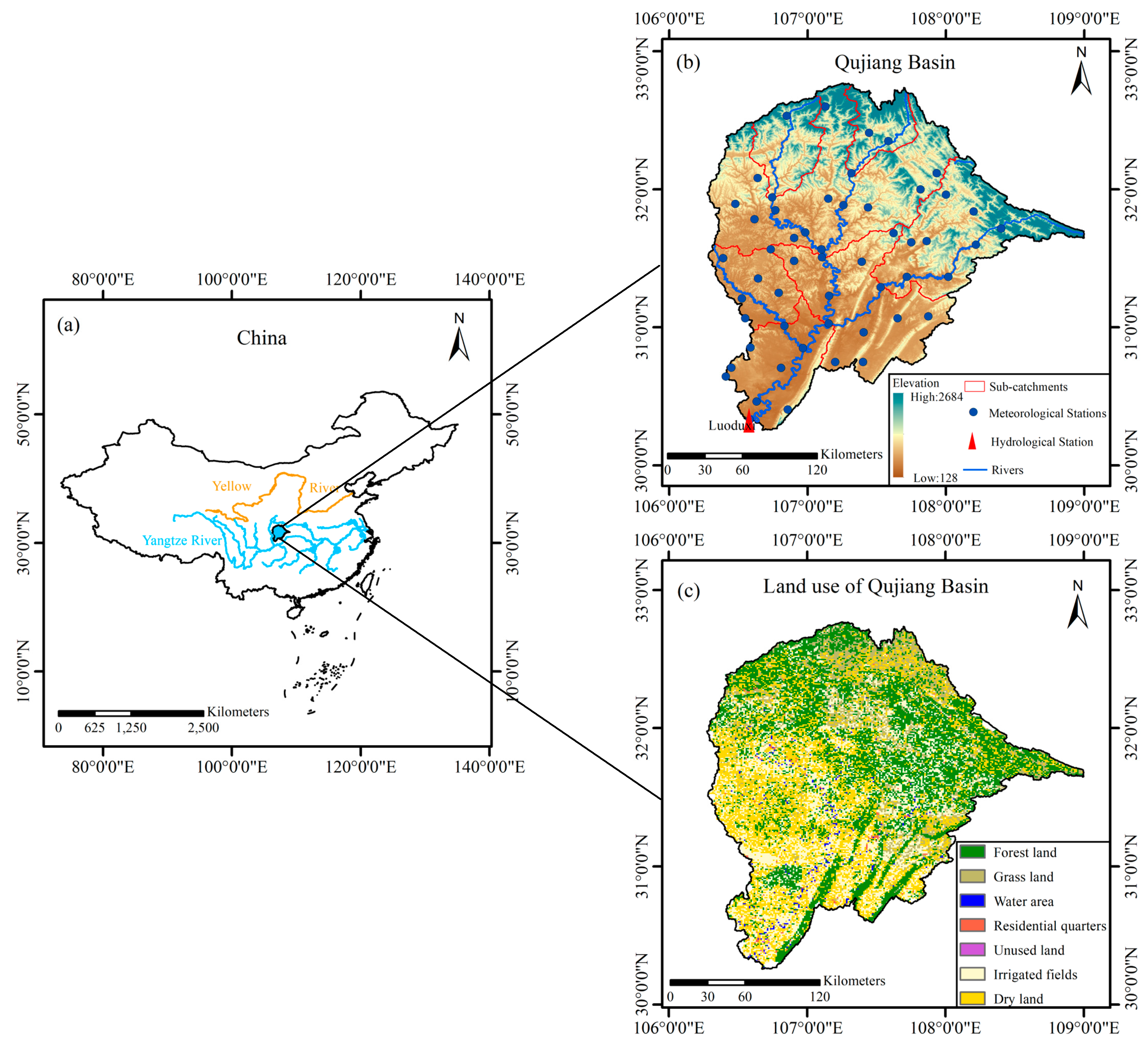
2.1. Study Area

The Qujiang catchment, located between 106°00′ E–109°00′ E and 30°00′ N–33°00′ N, is a typical humid catchment in southwestern China [35] with a drainage area of 39211 km² (Figure 1). It originates at Tiechuan Mountain situated at the juncture of the Shanxi and Sichuan Provinces of China and flows southwest to the Jialing River at the north of Chongqing. The catchment is divided into seven sub-catchments (circled by red lines in Figure 1b) based on the river networks, which are in accordance with the sub-catchments divided by DDRM when modelling the Qujiang catchment. The northern part of the catchment contains the Daba Mountain and Michang Mountain while the southern part is a plateau. The elevation within the Qujiang catchment ranges from 128 to 2684 m a.s.l., and decreases from northeast to southwest.

The Qujiang catchment is characterized by a subtropical monsoon climate. The middle and lower reaches of the catchment have moderate temperatures and abundant precipitation, while the temperature of the upper reaches is relatively low. The annual rainfall of the catchment ranges from 1014 to 1253 mm, and the annual rainfall in areas of Michang Mountain and Daba Mountain ranges from 1014–1500 mm. The rainy season in this catchment generally starts in April and ends in October. The annual runoff at the outlet station (Luoduxi station) is 23 billion m³, contributing about 30% of the Jialing River’s total discharge.

Vegetation covering varies greatly over time across the Qujiang catchment, as shown in Figure 2. The middle and lower reaches are covered mostly by cultivated and dry land, while the upper reaches are covered mostly by forest land, as shown in Figure 1b. According to the Harmonized World Soil Database (HWSD) [36], the soil texture across Qujiang catchment encompasses loamy, silt loamy, light clayey and loamy sand, and the great majority of the catchment has a loamy texture. The soil porosity values and soil (root-zone) depth values across Qujiang catchment are estimated by results of Saxton and Rawls, at around 0.46 and 100 cm, respectively [37].

2.2. Hydro-Meteorological Data

The hydro-meteorological data used in this study for hydrologic modelling include the daily discharge data from the Luoduxi hydrological station and daily meteorological data for the period of 2010–2016 (precipitation and mean air temperature data) from 53 meteorological stations, which are evenly distributed in the Qujiang catchment (Figure 1b). The daily meteorological data from 53 meteorological stations are obtained from the China Meteorological Data Sharing Service System developed by the National Climate Centre of China Meteorological Administration.

The Blaney-Criddle method is used to calculate potential evaporation, PET from daily mean air temperature data from the 53 meteorological stations [37]. The input data for DDRM are grid-based precipitation and PET. The Inverse Distance weighted method (IDW) is used for spatial interpolation of precipitation and PET to fit the discrete grids of DDRM [38]. In this study, the resolution of grids applied in DDRM is 1 km. The inputs of XAJ model are areal mean precipitation and PET data of Qujiang catchment, which are calculated as the overall averages from 53 stations. The output data of XAJ model are areal soil moisture averages across the Qujiang catchment from 2010 to 2016.

2.3. Remotely Sensed Soil Moisture Products

Four remotely sensed soil moisture products are used in the study, i.e., ASCAT-A, ASCAT-B, SMAP and SMOS. This study considers only ascending overpasses of satellites, which have a better spatial coverage of the study area.

The ASCAT, flying on the board of the polar-orbiting Meteorological Operational (MetOp) satellite series and using active microwave at a frequency of 5.255 GHz (C-band), was initially designed for monitoring winds over the oceans and was thought to be sub-optimal for soil moisture detection [39], but recent studies have shown that ASCAT soil measurements can be well suited for tracking changes on soil moisture [40] and have a positive impact in practical applications [41]. There are two available ASCAT products currently: the ASCAT-A was launched on the MetOp-A satellite in October 2006, which then became fully operational in May 2007 and continues to operate today, while the ASCAT-B instrument on the MetOp-B satellite became operational in September 2012. In the study, the raw ASCAT Surface Soil Moisture Level-2 (L2) products (ASCAT-A and ACAT-B) given in swath geometry are available from European Organization for the Exploitation of Meteorological Satellites (EUMETSAT) with a spatial sampling resolution of 12.5 km [41]. Retrievals are available at least once a day (in descending orbit and/or in ascending orbit), and a time-series based change-detection method to remove the adverse influence of surface roughness and eliminate the contribution of vegetation is used. ASCAT products provide a relative measurement of the soil moisture contents in the top 0.5–2 cm of the soil profile. The soil moisture information is derived and expressed as the saturation degree (%) of surface soil moisture, denoted by ${\omega }_{SSM}^{ASCAT}$, whose values for the historical highest and lowest measurements are 100% and 0% respectively. The porosity values are required to convert saturation degree ${\omega }_{SSM}^{ASCAT}$ to soil moisture contents given in m³ m⁻³, which are denoted by ${\theta }_{SSM}^{ASCAT}$. ASCAT-A product used in this study covers the period of January 2010 to December 2016, while ASCAT-B product covers the period of May 2013 to December 2016. In the study, the soil moisture data with a noise error (ERR) greater than 14% were screened out [42].

Launched in 31 January 2015, NASA’s SMAP satellite, which was specially designed for providing high tempo-spatial resolution global maps of soil moisture and landscape thaw/freeze state, is the newest L-band soil moisture dedicated satellite in orbit. It was initially designed to incorporate an L-band (1.26 GHz) active radar and an L-band (1.41 GHz) passive radiometer over large domains [9]. However, its active radar broke down in July 2015. In this paper, the SMAP enhanced Level-3 (L3) radiometer global surface soil moisture (${\theta }_{SSM}^{SMAP}$) product (version 1) sourced from the National Snow and Ice Data Center (NSIDC) is used [43]. This soil moisture product is based on the Single Channel Algorithm V-pol (SCA-V) [44]. It has an initial spatial resolution of nearly 36 km and is subsequently resampled to 9-km resolution by NSIDC with a sensing depth of the top 5 cm of the soil profile and covers the period after April 2015. In the study, only the SMAP soil moisture data that the Retrieval Quality Flag (RQF) recommended were used.

The SMOS, which is the first satellite designated for soil moisture acquisitions using fully polarized passive microwave observed at multiple angles, was launched in November 2009 by European Space Agency (ESA) [45]. The Microwave Imaging Radiometer uses Aperture Synthesis extracts L-Band microwave emissions (1.400–1.427 GHz) from Earth’s surface (0–5 cm of the soil) to map levels of soil moisture. The SMOS provides regular observations of a revisit time of nearly 3 days with a spatial resolution of 35–50 km. In this study, the surface soil moisture contents (${\theta }_{SSM}^{SMOS}$) given in percentage volumetric units (m³ m⁻³) are sourced from the ESA Level 2 processor based on the L-Band Microwave Emission of the Biosphere (L-MEB) model [46], namely SMOS operational Soil Moisture User Dara Product 2, version 6.50 (SMUDP2) and cover the period from June 2010. The product is available on hexagon grids of 15 km resolution over the Discrete Global Grid (DGG) [18]. For SMOS product, the soil moisture data were masked out if the Data Quality Index (DQX) is equal to 0 (filled value) or larger than 0.06, or the radio frequency interferences (RFI) are larger than 30% [47].

Before comparisons, raw ASCAT swath soil moisture products and SMOS DGG soil moisture product are resampled to gridded soil moisture through nearest resampling technique via ArcGIS without changing their spatial resolutions. The output grid value of the overlapping is the average of the overlapping grids. The spatial resolution of gridded soil moisture from ASCAT, SMAP and SMOS are 12.5 km, 9 km and 15 km respectively.

Table 1. Periods of satellite products chosen for this study.

Satellites	ASCAT-A	ASCAT-B	SMAP	SMOS
Period	2010.1–2016.12	2013.5–2016.12	2015.4–2016.12	2010.6–2016.12

presents the time periods of data chosen in the study of each remotely sensed soil moisture product.

The exponential filter proposed by Wagner et al. is adopted to define a soil water index (SWI) to represent the profile soil moisture contents for each remotely sensed soil moisture product. It is denoted by ${\theta }_{SWI}^{RS}$ with a unit of m³ m⁻³, under the assumption that the variation in time of the profile soil moisture is linearly related to the difference between the surface soil moisture and the profile soil moisture [48]. The recursive formulation is represented as follows:

$${\theta }_{SWI}^{RS}\left(t_n\right)={\theta }_{SWI}^{RS}\left(t_{n-1}\right)+K_n\left[{\theta }_{SSM}^{RS}\left(t_n\right)-{\theta }_{SWI}^{RS}\left(t_{n-1}\right)\right]$$

(1)

where time t_n indicates the acquisition time of surface soil moisture contents acquired from satellites, which are denoted by ${\theta }_{SSM}^{RS}$, and t_n−1 indicates the previous acquisition time. K_n is the gain term at the acquisition time t_n varying between 0 and 1 as follows:

$$K_n=\frac{K_{n-1}}{K_{n-1}+e^{-\left(\frac{t_n-t_{n-1}}{T}\right)}}$$

(2)

where T is the characteristic time length representing the timescale of soil moisture variation, which is calculated by maximizing the correlation between the soil water index and the model-simulated soil moisture. For the initialization of the filter, K₁ is set to 1.

3. Methodology

In this section, the XAJ model and the DDRM are first presented in details to explain how to simulate catchment-averaged soil moisture values as well as the spatial distribution of soil moisture values. Then, methodology of comparisons, the correlation coefficient R and the root mean square difference RMSD used in comparison study are described.

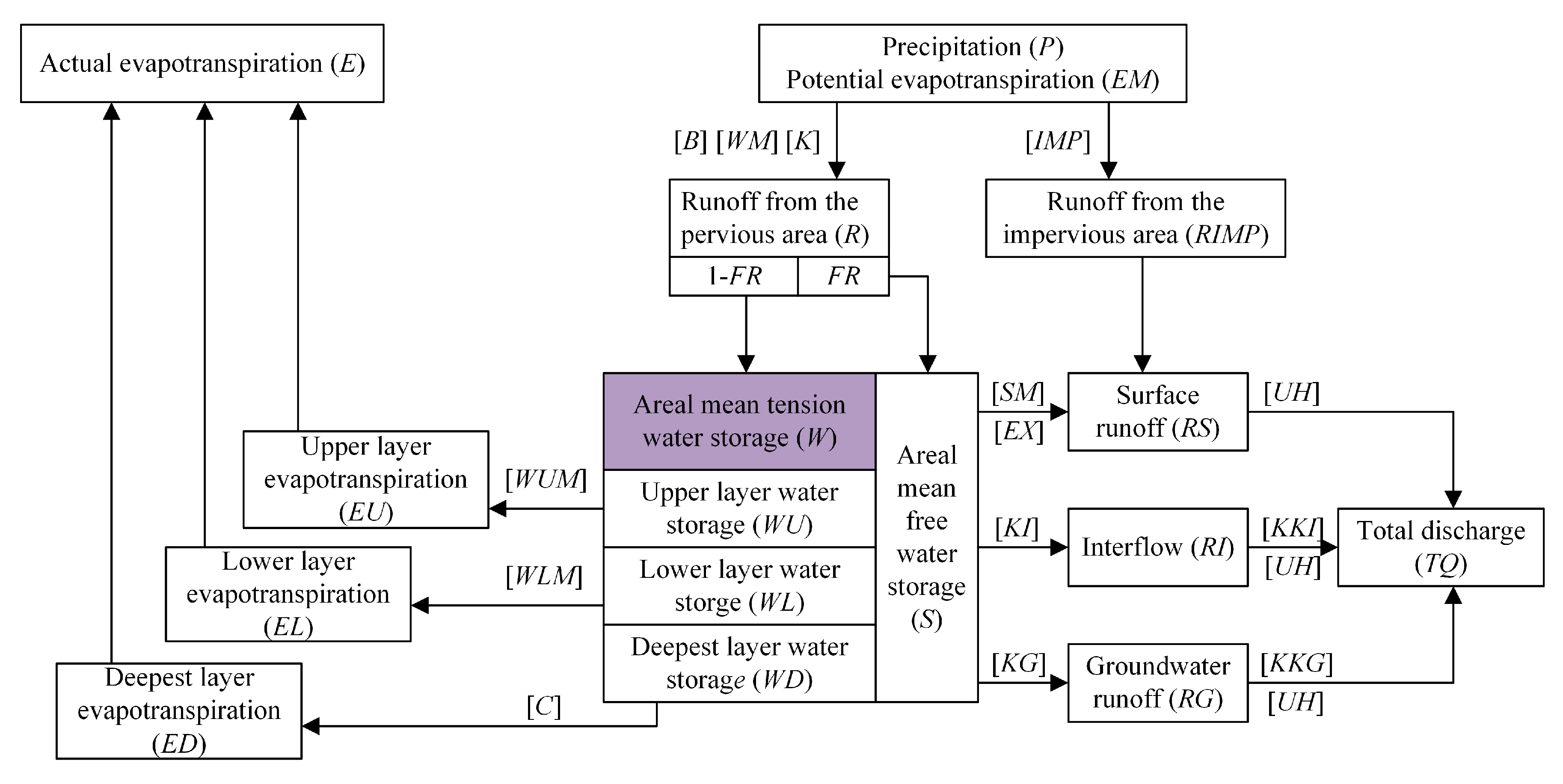
3.1. The Xinanjiang (XAJ) Model

3.1.1. Model Structure

The XAJ model is a widely-used conceptual hydrological model for flood forecasting in China [15]. It can provide accurate flow predictions in humid and semi-humid regions where saturation excess runoff dominates [49]. This model consists of four calculation components, including evapotranspiration, runoff generation, runoff separation and flow concentration. As Figure 3 shows, the XAJ model divides the vertical soil depth into three layers, i.e., upper layer, lower layer and deepest layer. In the runoff producing area, three soil layers will generate the respective runoff components, i.e., surface runoff, interflow and groundwater. For each of three layers, its soil moisture content changes due to evapotranspiration and possible runoff. For this model, runoff production occurs only at points where the tension water storage is replete, thus a distribution curve of tension water capacity across the catchment is built to calculate the spatial distribution of the tension water storage. The calculation of the interflow and the groundwater flow is based on the linear reservoir method. A unit hydrograph is used to calculate runoff concentration. More details of the XAJ model are shown in [15].

3.1.2. Model Parameters

The lumped XAJ model has 13 parameters and a dimensionless unit hydrograph UH. They can be classified into evapotranspiration parameters (K, WUM, WLM, C), runoff generation parameters (WM, B, IMP, SM, EX, KI, KG) and routing parameters (KKI, KKG).

All the parameters are estimated by the Shuffled Complex Evolution (SCE-UA) method, which combines the strengths of multiple methods and has good performance in parameter calibration [50]. A widely used performance criterion Nash-Sutcliffe Coefficient of Efficiency (NSE) is chosen as the objective function. More details about XAJ model parameters are shown in

Table 2. Descriptions of the XAJ model parameters.

Parameters	Unit	Prior Ranges	Description	Optimized Values
K	-	0.5–1	The ratio of potential evapotranspiration to pan evapotranspiration	0.52
IMP	-	0–0.3	The fraction of the impervious area of the catchment	0.01
B	-	0–0.5	A parameter relating to the distribution of tension water capacity	0.40
WM	mm	100–700	Areal mean free water storage capacity	272.32
WUM	mm	30–100	Upper layer water storage capacity	10.01
WLM	mm	10–90	Lower layer water storage capacity	62.29
C	-	0.08–0.3	A factor of remaining potential evaporation in the deepest layer	0.24
SM	mm	10–50	Areal mean free water storage capacity	34.76
EX	-	0.5–2	A parameter relating to the distribution of free water storage capacity	0.99
KG	-	0–0.45	A coefficient relating to a contribution to groundwater storage	0.08
KI	-	0–0.35	A coefficient relating a contribution to interflow storage	0.13
KKG	-	0–1	The groundwater reservoir constant	0.99
KKI	-	0–0.9	The interflow reservoir constant	0.86

.

3.1.3. Calculation of Soil Moisture

In the XAJ model, the variable W (purple-shaded in Figure 3) is the sum of soil moisture storage depths of three soil layers, i.e., W = WU + WL + WD, and is more likely to represent the profile soil moisture. This variable is given in a single storage depth (mm), representing the daily catchment-averaged soil moisture, and can convert to the soil moisture content θ^XAJ (m³ m⁻³) when catchment-averaged soil depth (D) is given, which can be represented as:

$${\theta }^{XAJ}=\frac{W\cdot A}{D\cdot A}=\frac{W}{D}$$

(3)

where A (m²) represents the whole catchment area.

3.2. The DEM-Based Distributed Hydrological Model

The DEM-based distributed hydrological model (DDRM) was proposed by Xiong et al. and has been used in the humid and semi-humid regions for flood forecasting in southern China [17,51,52,53]. In the model, a big catchment will be divided into a number of sub-catchments, and each sub-catchment is represented by a number of DEM grids, with the outlets of each sub-catchment are connected to constitute the river networks of the total catchment, as demonstrated by Figure 4. The DDRM has three calculation components: grid excess rainfall calculation, sub-catchment outlet streamflow calculation, and streamflow routing through the river network.

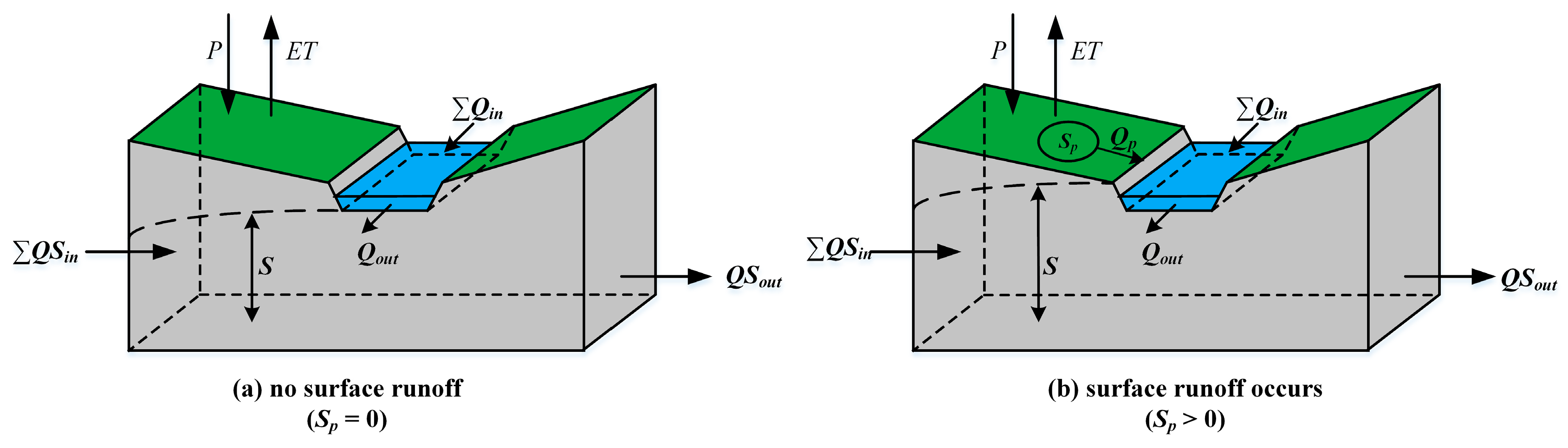
3.2.1. Grid Excess Rainfall Calculation

Grid excess rainfall is largely influenced by soil water storage in each grid. For the DDRM, soil water storage capacity (S_mc) differs from grids to grids. The DDRM establishes linkages between S_mc and the corresponding topographic index ln(α/tanβ) at grid i by the following relationship:

$$S_{mc,i}=S_0+SM\cdot {\left\{\frac{\ln {\left(\alpha /\tan \beta \right)}_i-\underset{j}{\min }\left[\ln {\left(\alpha /\tan \beta \right)}_j\right]}{\underset{j}{\max }\left[\ln \left(\alpha /\tan \beta \right)\right]-\underset{j}{\min }\left[\ln {\left(\alpha /\tan \beta \right)}_j\right]}\right\}}^a$$

(4)

where S₀ and SM respectively represent the minimum water storage capacity of the catchment and the range of water storage capacity across the catchment, a denotes as an empirical index that can be acquired by calibration.

For grid i of DDRM, the actual evapotranspiration ET_i is calculated by:

$$E{T}_i=\frac{S_i}{S_{mc,i}}PE{T}_i$$

(5)

where S_i is the actual soil moisture storage, and PET_i represents potential evapotranspiration.

The inflow of groundwater QS_in,i and the outflow of groundwater QS_out,i for grid i can be calculated as:

$$Q{S}_{in,i}={\displaystyle \sum _{}^{}Q{S}_{out,j}}$$

(6)

$$Q{S}_{out,i}=\frac{\max \left\{\left(S_i-S{T}_i\right),0\right\}}{T_s}\cdot {\left[\tan \left({\overline{\beta }}_i\right)\right]}^b$$

(7)

where QS_out,j represents the groundwater outflow from the surrounding upstream grids j of grid $i$. ST_i is the residual groundwater and can be considered as a constant portion a of S_mc,i, where a is an empirical parameter. T_s is a time constant reflecting the underground flow properties of grid i. $\tan \left({\overline{\beta }}_i\right)$ stands for the average slope across the study area. T_s and b are model parameters acquired by model calibration. Soil moisture storage S_i can be calculated as:

$$S_i\left(t\right)=S_i\left(t-\Delta t\right)+\left[P_i\left(t\right)-E{T}_i\left(t\right)\right]\cdot \Delta A\cdot \Delta t+\left[Q{S}_{in,i}\left(t\right)-Q{S}_{out,i}\left(t\right)\right]\cdot \Delta t$$

(8)

where t denotes time, Δt denotes time step, P_i is precipitation, and ΔA is the grid area. Runoff generation in each grid of DDRM is based on saturation excess runoff mechanism. Where the soil is unsaturated, i.e., S_i < S_mc,i, there is no excess rainfall generated to replenish the surface ponding water storage S_p,i (Figure 5a). When S_i > S_mc,i (Figure 5b), S_p,i will be replenished and updated as follows:

$$S_{p,i}\left(t\right)=S_{p,i}\left(t-\Delta t\right)+\max \left\{S_i\left(t\right)-S_{mc,i},0\right\}$$

(9)

Then the grid excess rainfall generation rate Q_p,i is generated from S_p,i and calculated under the linear reservoir assumption as:

$$Q_{p,i}=S_{p,i}/T_p$$

(10)

where T_p is a time constant estimated by model calibration.

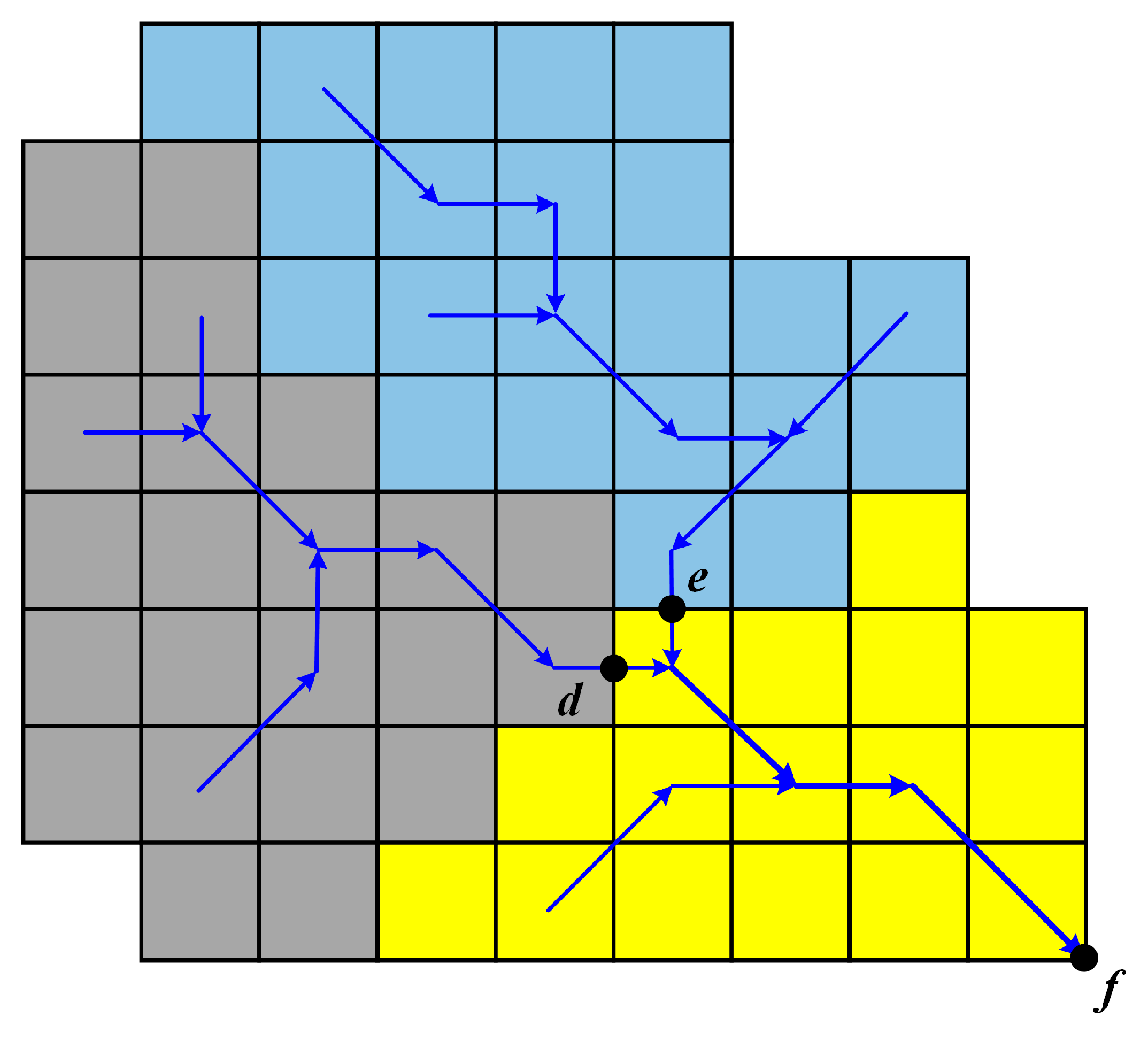
3.2.2. Sub-Catchment Outlet Streamflow Calculation by Grid Channel Routing

As shown in Figure 4, DDRM divides catchment into a number of sub-catchments according to requirements. Within each sub-catchment, the Muskingum method is used to route the grid excess rainfall generation rate Q_p,i through grids one by one from upstream to downstream in order to finally get the streamflow values at the sub-catchment outlet. For grid i, the routed streamflow is denoted as Q_out,i, which is expressed as:

$$Q_{out,i}\left(t\right)=c_0\left[Q_{in,i}\left(t\right)+Q_{p,i}\left(t\right)\right]+c_1\left[Q_{in,i}\left(t-\Delta t\right)+Q_{p,i}\left(t-\Delta t\right)\right]+c_2{Q}_{out,i}\left(t-\Delta t\right)$$

(11)

where c₀, c₁ and c₂ are grid channel parameters of the Muskingum method, which are all between 0 and 1, and their sum equals 1. The D8 algorithm, which is probably the most popular algorithm for automated drainage recognition, is used in this model to determine the sequence of channel routing across all the grids within the sub-catchment [54].

3.2.3. Streamflow Routing through River Networks

Streamflow from all sub-catchment outlets is further routed through the river networks also by the Muskingum method. As Figure 4 shows, a big catchment consists of multiple sub-catchments. The discharge at the outlet f of the whole catchment, denoted by O^f, contains three components, i.e., O^df, the discharge routed from the streamflow at the sub-catchment outlet d; O^ef, the discharge routed from the streamflow at the sub-catchment outlet e; and O_out,f, the discharge at the sub-catchment outlet f that is generated only from the rainfall falling on the sub-catchment 3. Thus O^f is expressed as follows:

$$O^f\left(t\right)=O^{df}\left(t\right)+O^{ef}\left(t\right)+O_{out,f}\left(t\right)$$

(12)

$$O^{df}\left(t\right)=h{c}_0^{df}{O}^{df}\left(t-\Delta t\right)+h{c}_1^{df}{Q}_{out,d}\left(t\right)+h{c}_2^{df}{Q}_{out,d}\left(t-\Delta t\right)$$

(13)

$$O^{ef}\left(t\right)=h{c}_0^{ef}{O}^{ef}\left(t-\Delta t\right)+h{c}_1^{ef}{Q}_{out,e}\left(t\right)+h{c}_2^{ef}{Q}_{out,e}\left(t-\Delta t\right)$$

(14)

where O_out,d and Q_out,e represent streamflow at sub-catchment outlets d (sub-catchment 1) and e (sub-catchment 2) respectively, while $h{c}_0^m$, $h{c}_1^m$ and $h{c}_2^m$ (m represents df or ef) are the river network routing parameters of Muskingum method.

3.2.4. Model Parameters

The DDRM has 10 parameters, including runoff generation parameters (S₀, SM, T_s, T_p, a, b), grid channel routing parameters c_i (i = 0,1), and the river networks routing parameters $h{c}_i^m\left(i=0,1\right)$, m represents the routing processes of streamflow from the outlets of different sub-catchments. In the study, only one set of river networks’ routing parameters is used. Like in the XAJ model, all the parameters are calibrated by SCE-UA method. More details about DDRM model parameters are shown in

Table 3. Descriptions of the DDRM parameters.

Parameters	Unit	Prior Ranges	Description	Optimized Values
S0	mm	5–100	Minimum water storage capacity	96.35
SM	mm	5–500	Range of water storage capacity across the catchment	498.49
Ts	h	2–200	Time constant, reflecting the characteristic of groundwater	112.89
Tp	h	2–200	Time constant, reflecting the characteristic of surface flow	27.70
a	-	0–1	Empirical parameter, reflecting the characteristic of ground outflow	0.10
b	-	0–1	Empirical parameter, reflecting the relationship between Smc and corresponding topographic index	0.98
c0	-	0–1	A grid channel parameter of the Muskingum method	0.98
c1	-	0–1	A grid channel parameter of the Muskingum method	0.01
$h{c}_0^m$	-	0–1	River networks routing parameters of Muskingum method	0.09
$h{c}_1^m$c1	-	0–1	River networks routing parameters of Muskingum method	0.46

.

3.2.5. Calculation of Soil Moisture

For the DDRM, the soil moisture storage depth S_i of grids (given in mm), which is comparable to the profile soil moisture, is chosen to make comparisons with the remotely sensed gridded soil moisture in the study. This variable plays an important role in simulating the runoff generation of each grid of DDRM. Moreover, daily catchment-averaged soil moisture is also calculated based on gridded soil moisture. Similar with the XAJ model, $S_i$ can be converted to the soil moisture contents ${\theta }_i^{DDRM}$, which is calculated as:

$${\theta }_i^{DDRM}=\frac{S_i\cdot A_i}{D_i\cdot A_i}=\frac{S_i}{D_i}$$

(15)

where ${\theta }_i^{DDRM}$ is the model-simulated soil moisture of grid i given in m³ m⁻³, and D_i and A_i are the soil depth and grid area of grid i.

3.3. Methodology of Comparisons

Although all remotely sensed and model-simulated soil moisture can be converted to soil moisture contents (θ) when soil porosity values and soil (root-zone) depth values are given, the error of estimation of θ is probably large, since soil texture characteristics are highly simplified due to the scarcity of soil data. Thus, all soil moisture datasets are rescaled between 0 to 1 using a minimum-maximum correction technique [42], showing as saturation degree (ω) to allow for robust comparisons. There is no physical meaning for saturation degree in fact, it is only a relative value. Previous studies have rescaled soil moisture using this technique when they used multiple remotely sensed soil moisture datasets with different units [55,56].

Before comparing with the model-simulated soil moisture, catchment-wide averages of four remotely sensed soil moisture products are directly compared with each other firstly, which can give a preliminary assessment of their consistencies. The lumped XAJ model-simulated soil moisture and DDRM catchment-wide soil moisture averages are compared with catchment-wide averages of remotely sensed soil moisture for the whole period, the dormant seasons and the growing seasons respectively. It aims to evaluate the overall consistencies over the whole study area, and also evaluate the seasonal effect on the consistencies. Besides, direct comparisons of their time series have also been attempted to check the soil moisture evolution with time.

Only DDRM model-simulated soil moisture can compare with distributed remotely sensed soil moisture to evaluate consistencies of their spatial distributions. Since satellite products have different spatial resolutions (SMAP-15 km, ASCAT-12.5 km, SMOS-15 km), while the study area is divided into 1 km grids with DDRM modelling, gridded DDRM soil moisture of 1 km is resampled to match the resolution of each satellite product before comparisons. The consistency of soil moisture in each grid has been evaluated for the whole period, the dormant seasons and the growing seasons, while regional effect on their consistencies can also been shown. This kind of comparisons provides more details about their consistencies than only comparing their catchment-wide averages. For each remotely sensed soil moisture product, the highest, mean and lowest correlations across the study area have been shown and their corresponding soil moisture time series are compared to check the soil moisture evolution of characteristic grids with time.

3.4. Indexes for Soil Moisture Comparisons

In this study, two widely used indexes, the correlation coefficient R and the root mean square difference RMSD are used for comparisons. The first index R is defined as:

$$R\left({\omega }^{pro1},{\omega }^{pro2}\right)=\frac{{\displaystyle \sum _{t=1}^T\left({\omega }^{pro1}\left(t\right)-\overline{{\omega }^{pro1}\left(t\right)}\right)\times \left({\omega }^{pro2}\left(t\right)-\overline{{\omega }^{pro2}\left(t\right)}\right)}}{\sqrt{{\displaystyle \sum _{t=1}^T{\left({\omega }^{pro1}\left(t\right)-\overline{{\omega }^{pro1}\left(t\right)}\right)}^2}\times {\displaystyle \sum _{t=1}^T{\left({\omega }^{pro2}\left(t\right)-\overline{{\omega }^{pro2}\left(t\right)}\right)}^2}}}$$

(16)

where ω^pro1(t) and ω^pro2(t) are the saturation degrees on day t obtained from products pro1 and pro2, respectively, T is the total number of days during the period of comparison. To investigate the statistical significance of the correlation between products pro1 and pro2, the p-value (a measure of the correlation significance) is also calculated.

The second index RMSD is defined as:

$$RMSD\left({\omega }^{pro1},{\omega }^{pro2}\right)=\sqrt{\frac{1}{T}{\displaystyle \sum _{t=1}^T{\left({\omega }^{pro1}\left(t\right)-{\omega }^{pro2}\left(t\right)\right)}^2}}$$

(17)

Since both soil moisture datasets are not considered as actual soil moisture, this study uses the RMS difference terminology instead of RMS error (RMSE).

4. Results and Discussion

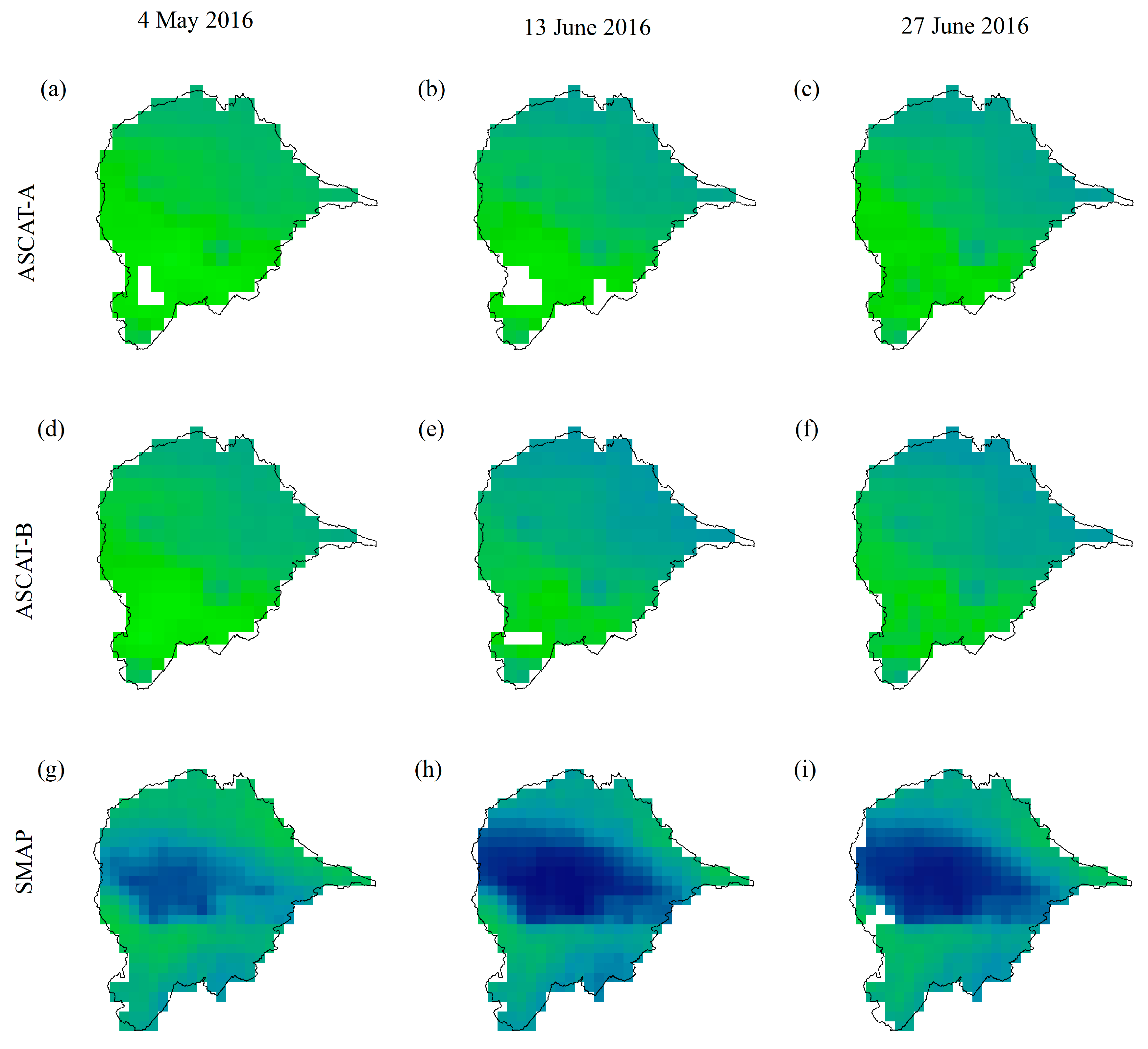
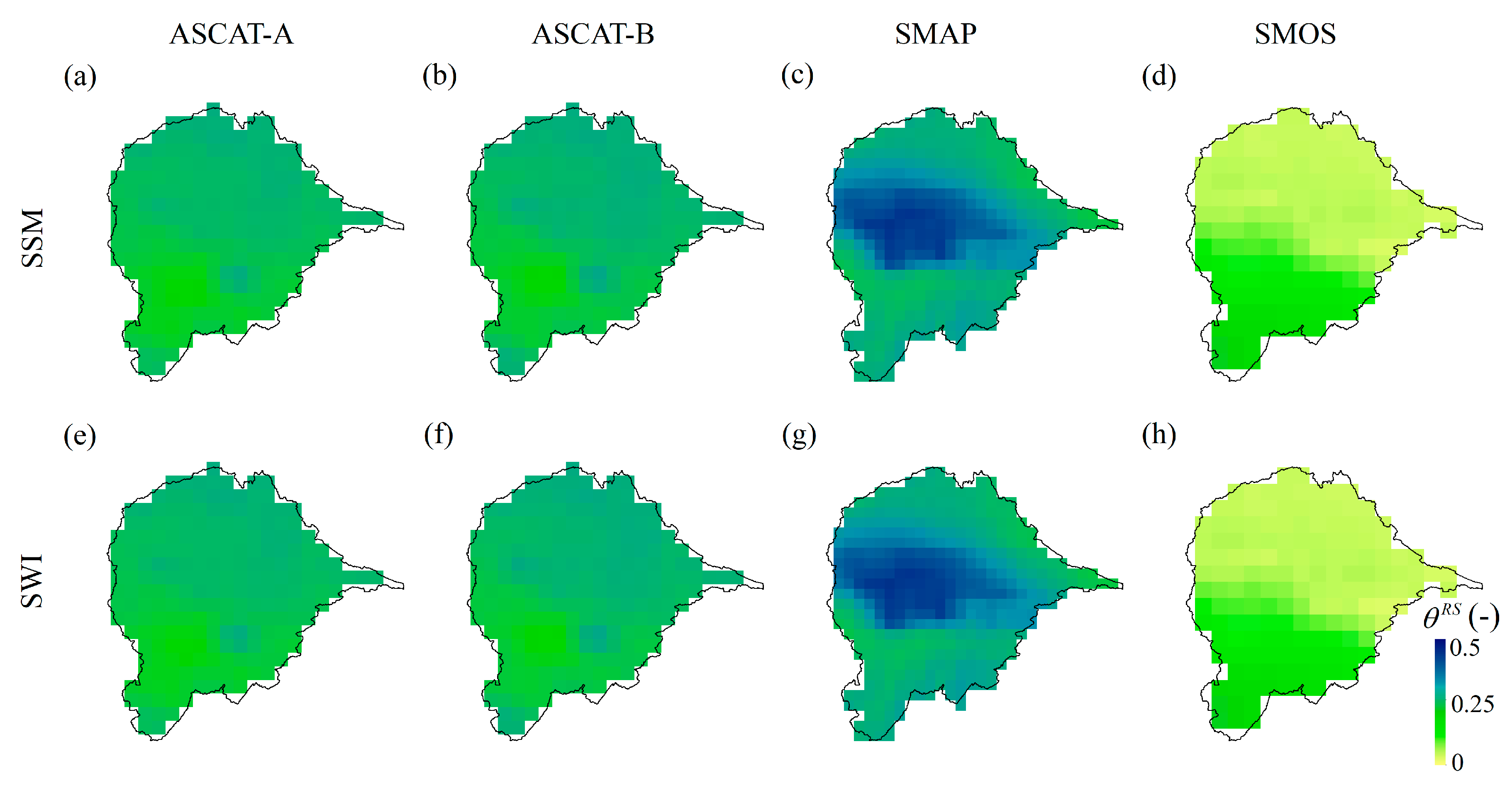
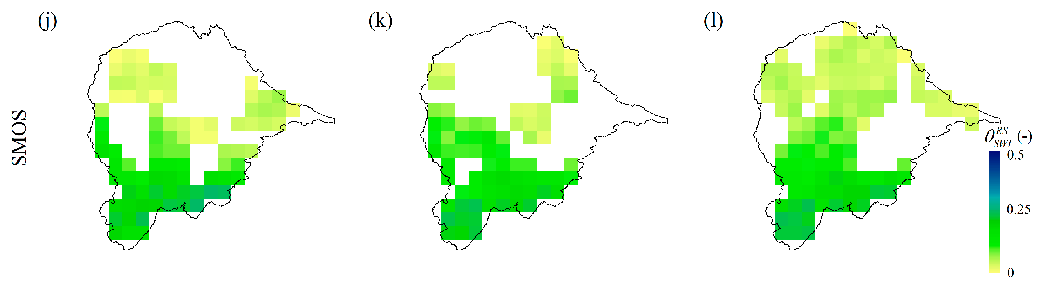
4.1. Remotely Sensed SSM and SWI from Satellites

All surface soil moisture (SSM) information across the Qujiang catchment is acquired from remotely sensed soil moisture products. The evaluation of SWI data is obtained from maximizing the overall correlation coefficient R between catchment-wide remotely sensed averages and model-simulated averages by varying the T parameter of the exponential filter from 1 to 100 days at a step of 1 day. This T value, which equals to 20 days, is applied to different sensors (ASCAT, SMAP and SMOS) and is used to calculate SWI to be compared to different models (the XAJ and DDRM). The estimated parameter T value is similar to the results of Wagner et al. who found T was 20 days for the 0–100 cm layer, and within the optimized characteristic time length obtained by Albergel et al. for soils with lower depth (around 50 cm soil depth with T around 20 days) [48,57].

Figure 6 presents averaged gridded surface soil moisture contents ${\theta }_{SSM}^{RS}$ and gridded soil wetness index ${\theta }_{SWI}^{RS}$ over the whole period of the different remotely sensed products. Figure 7 presents the profile soil moisture contents ${\theta }_{SWI}^{RS}$ from satellites across the Qujiang catchment on three specific days during a water-rising stage of 2016. It can be seen from Figure 6 that averaged ${\theta }_{SSM}^{SMAP}$ values are higher than averaged ${\theta }_{SSM}^{ASCAT}$ and ${\theta }_{SSM}^{SMOS}$ values, and soils of high altitudes are wetter than soils of lower altitudes for SMAP and ASCAT products. In contrast, SMOS product may underestimate soil moisture in mountain areas on these days, since soil moisture in high altitudes are significantly lower than those in lower altitudes. This may due to the fact that mountain areas of the Qujiang catchment affected by RFI experience either data loss or an underestimation in the retrieved geophysical parameters [58], since there are only around 200 soil moisture retrievals in high altitudes and around 400 soil moisture retrievals in lower altitudes, and the SMOS underestimates soil moisture due to the strong RFI in southwest China [59].

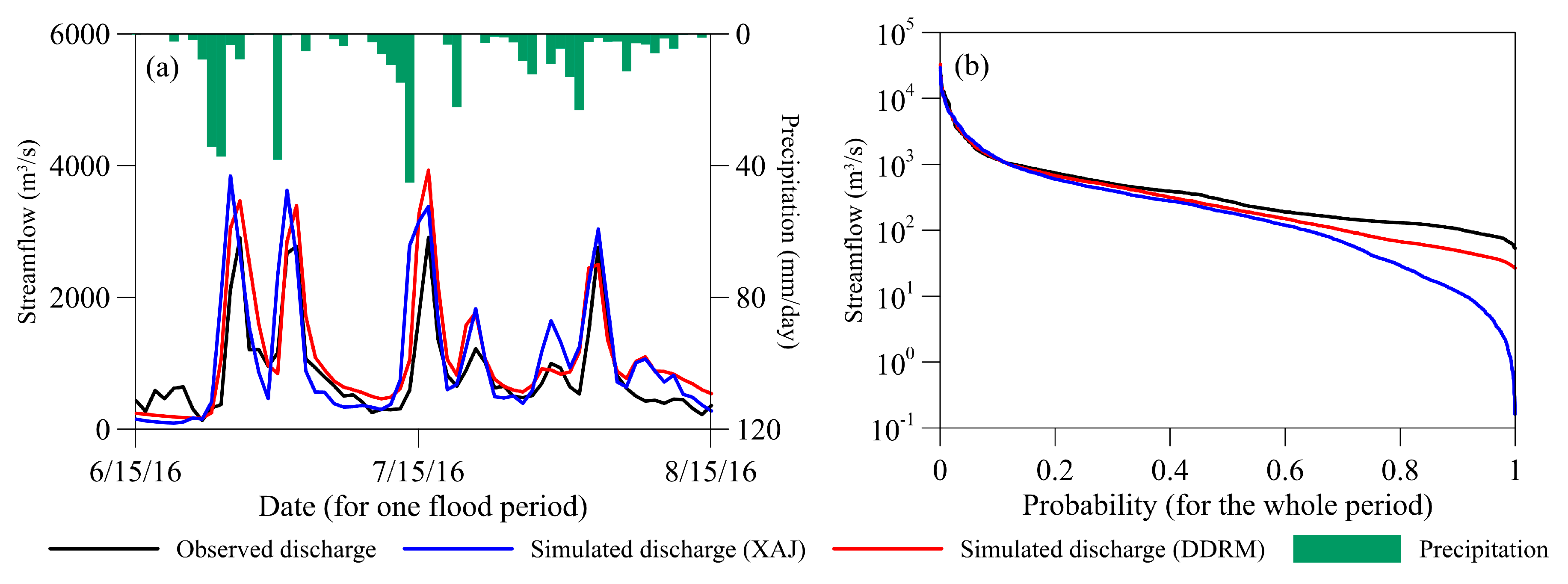
4.2. Simulations of Runoff and Soil Moisture Content by Hydrological Models

The observed discharge at the outlet of the Qujiang catchment during the period of 2010–2016 is used to calibrate parameters for both the XAJ model and the DDRM. Figure 8 presents the observed and simulated discharge time series acquired from the XAJ model and the DDRM respectively during the flood time period in 2016, as well as the daily flow duration curve of observed and simulated discharges for the whole time period of 2010–2016.

4.2.1. The XAJ Model

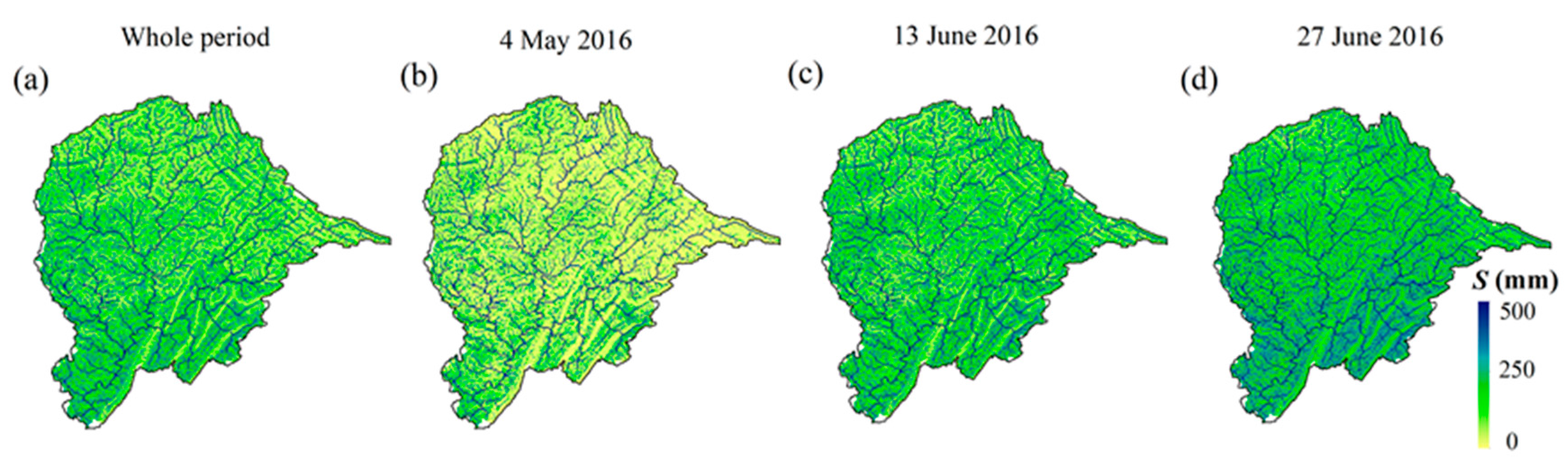
Table 2 presents the optimized parameter values for the XAJ model, the catchment-averaged soil moisture storage capacity WM is 272.32 mm, and the variable W of the XAJ model ranges from 153.53 mm to 272.32 mm. The NSE between the observed and simulated discharge for XAJ model during the whole period, the dormant season (from November to March) and the growing season (from May to October) of 2010–2016 is 0.85, 0.29 and 0.86 respectively. It reveals that XAJ model performs well during the growing seasons of 2010–2016, but poor during the dormant seasons, since the objective function NSE focuses more on high flows, which normally occur in the growing seasons rather than the dormant seasons in the Qujiang catchment. As shown in Figure 8, the XAJ model overestimates some flood peaks, and consistently underestimates some low flows. The prediction error for XAJ model may due to the error of input data and the lumped model structure, since the spatial heterogeneity of precipitation and soil moisture storage across the catchment is ignored when running a lumped hydrological model for the entire huge catchment.

4.2.2. The DDRM

The optimized parameter values for the DDRM are presented in Table 3. The soil moisture storage capacity of DDRM grids across Qujiang catchment ranges from 96.35 mm to 594.84 mm. The NSE between the observed and simulated discharge for the DDRM during the whole period, the dormant season and the growing season of 2010–2016 is 0.85, 0.63 and 0.82 respectively. Obviously, the DDRM performs better than the XAJ model during dormant seasons. As shown in Figure 8, there are some mismatches between calibrated DDRM and observed discharges. A key factor for prediction error in the DDRM is the low density of rainfall gauges across the catchment, which can lead to low quality gridded precipitation data. Another factor to consider is the simplification of runoff generation processes across the catchment. Besides, both models use Blaney-Criddle methodology for calculating PET, which has limitation and may result in uncertainty of the PET in the study area, and then leads to over or under estimations of soil moisture.

The catchment-averaged soil moisture storage depth calculated based on gridded soil moisture S_i ranges from 112.37 mm to 277.17 mm during 2010 to 2016. This range is similar to that of XAJ model, which means soil moisture simulated by the XAJ model and the DDRM probably represents soil moisture of similar soil depth. Figure 9 presents overall soil moisture averages over the whole period of DDRM modelling and soil moisture storage depth values simulated by DDRM on three specific days during a water-rising stage of 2016.

According to HWSD, soil depth values across the Qujiang catchment can be simplified to 100 cm. In this section, soil moisture storage depth S simulated by the DDRM is converted to θ^DDRM for the preliminary comparison with ${\theta }_{SSM}^{RS}$ and ${\theta }_{SWI}^{RS}$. A comparison of Figure 7 and Figure 9 indicates that satellites provide slightly higher soil moisture values than the DDRM, probably due to the over-simplified soil depth values when estimating θ^DDRM across the Qujiang catchment. Besides, the DDRM simulates wetter soil in lower altitudes, and this result conflicts with that of satellites. The reason for the difference may be that gridded soil moisture storage capacity values of the DDRM depending on topographic index tend to be higher in lower areas, similar to other models based on topographic index, such as TOPMODEL-based Land-Atmosphere Transfer Scheme (TOPLATS) [60].

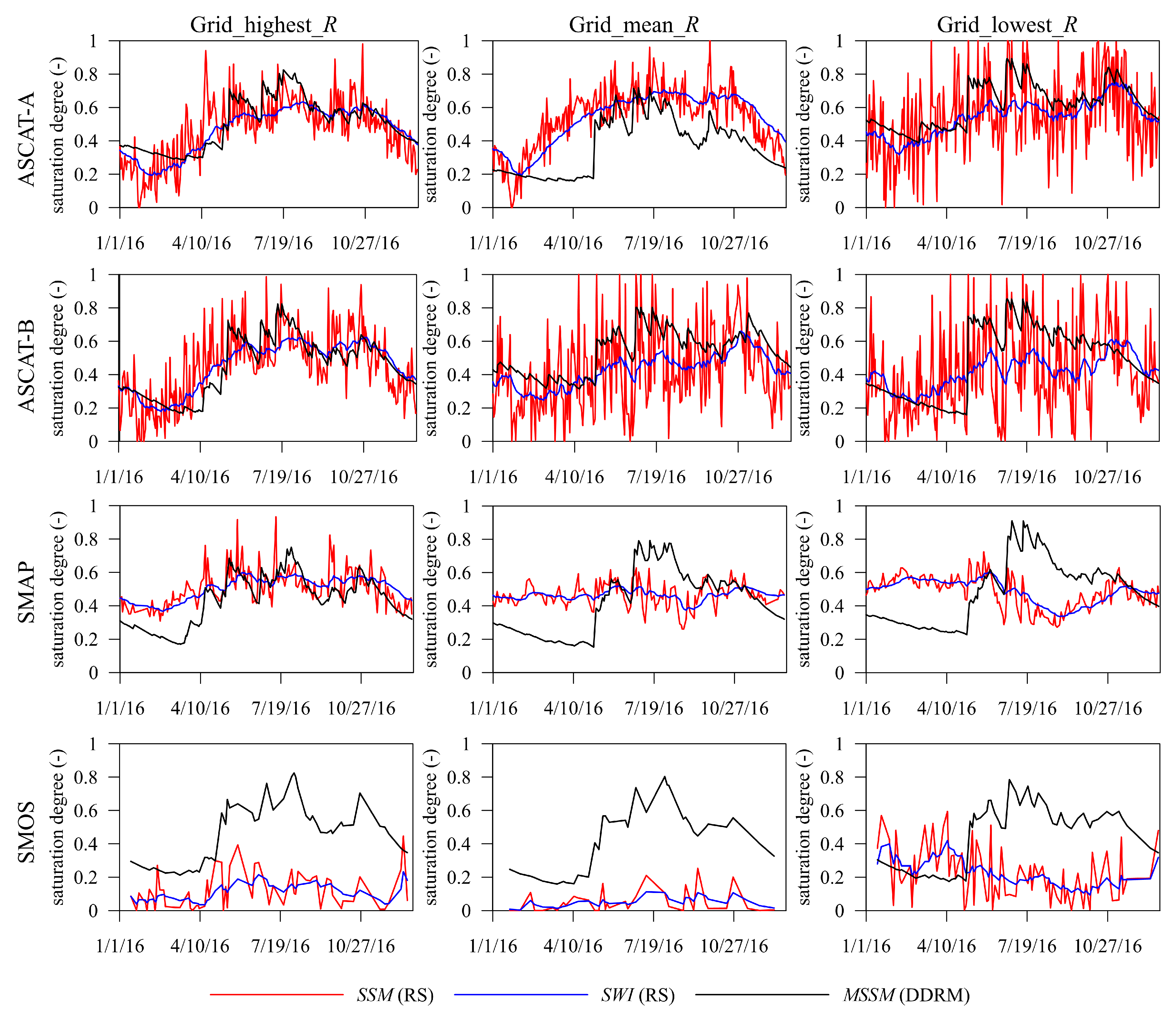
4.3. Comparisons of the Remotely Sensed and Model-Simulated Soil Moisture

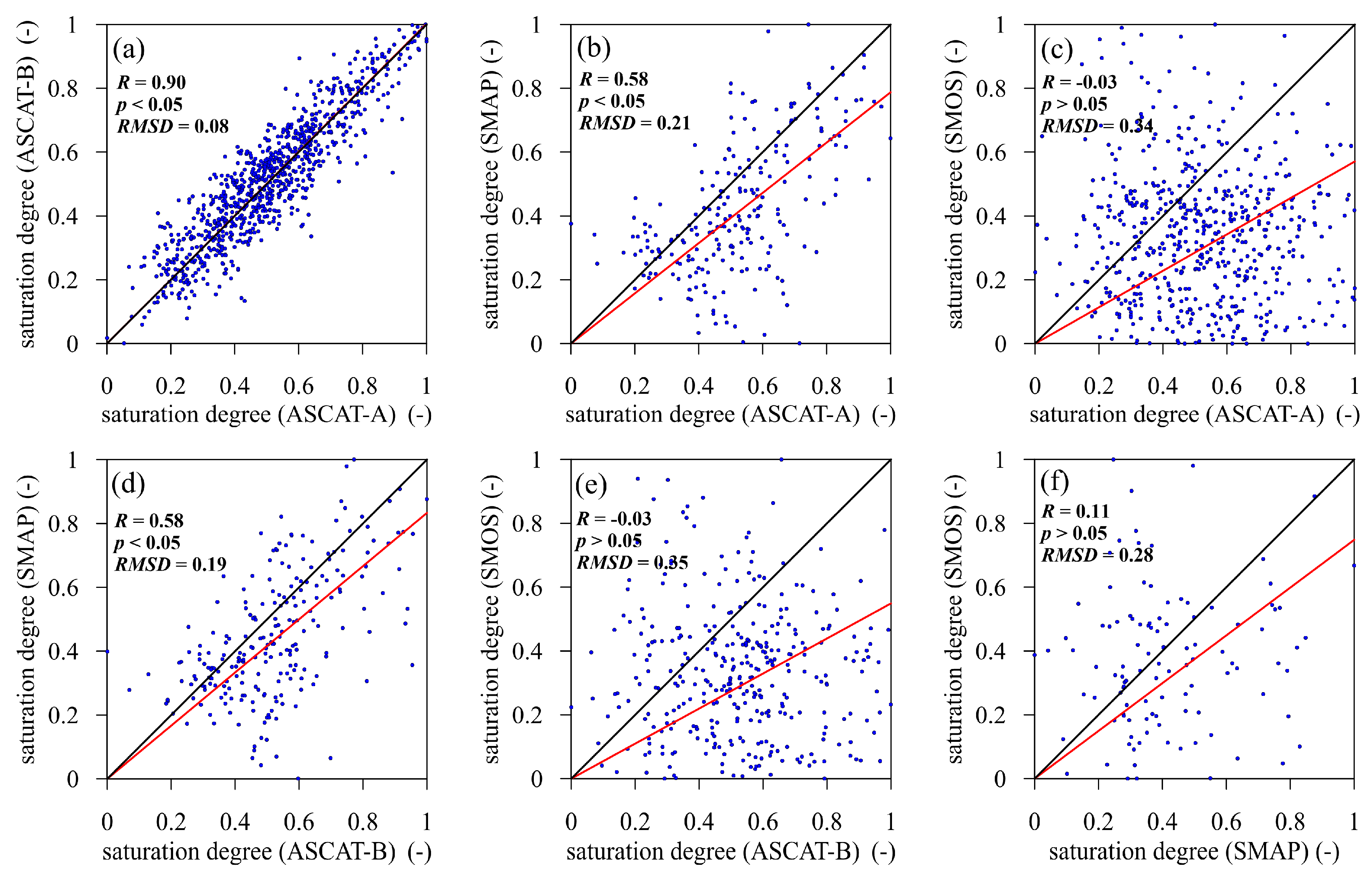
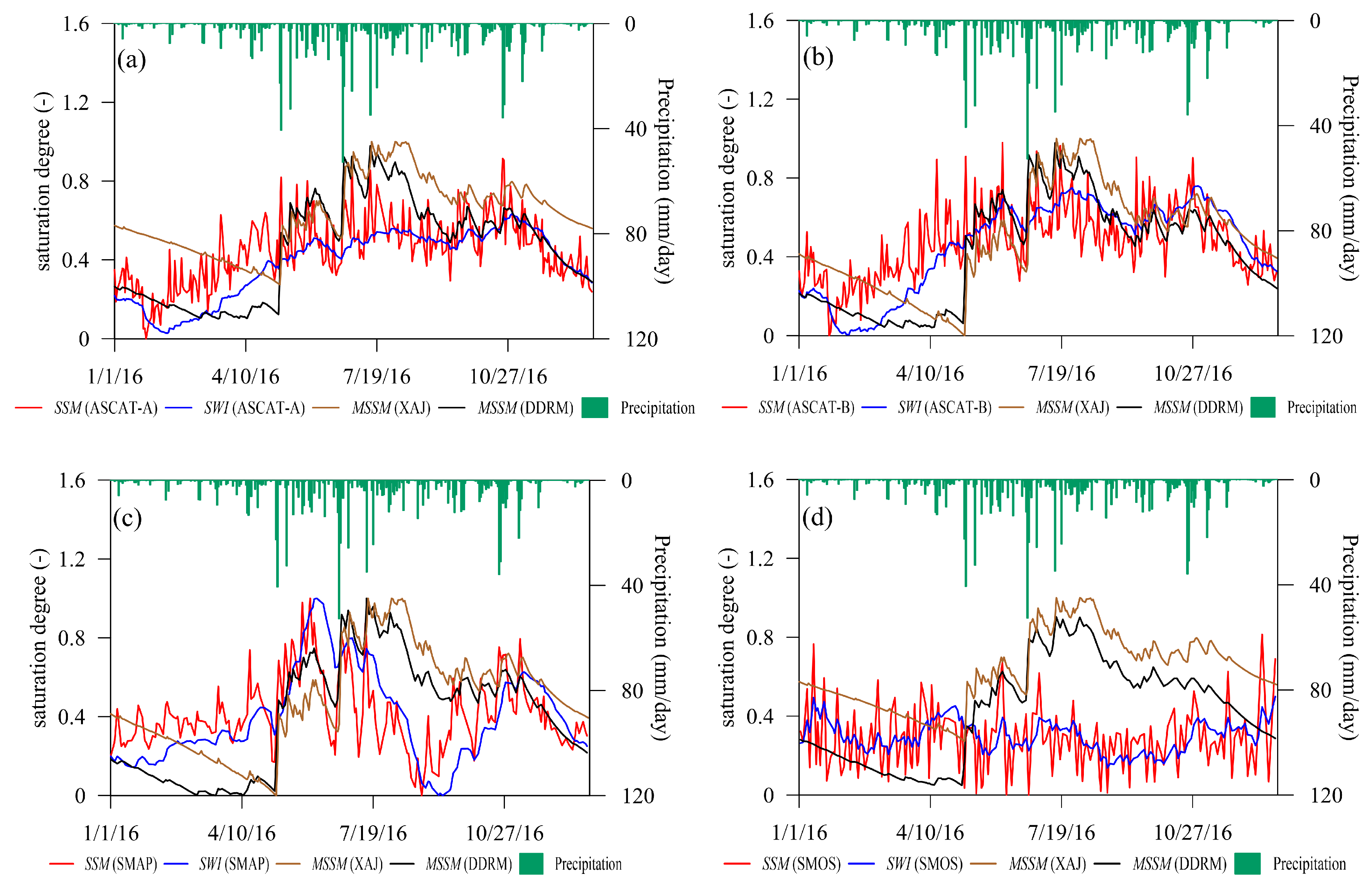
4.3.1. Catchment-Wide Average Values

In this section, the remotely sensed and the model-simulated catchment-averaged soil moistures across the Qujiang catchment are considered. Figure 10a–f present the correlations between the catchment-averaged ${\omega }_{SSM}^{RS}$ from different satellites. Since ASCAT-A and ASCAT-B soil moisture products are based on the same retrieval algorithm, ${\omega }_{SSM}^{ASCAT-A}$ and ${\omega }_{SSM}^{ASCAT-B}$ show the highest correlation coefficient at 0.90 with low RMSD of 0.08 (Figure 10a). The correlation coefficient of ${\omega }_{SSM}^{ASCAT-A}$ and ${\omega }_{SSM}^{SMAP}$, as well as that of ${\omega }_{SSM}^{ASCAT-B}$ and ${\omega }_{SSM}^{SMAP}$ are both 0.58 with RMSD of around 0.2 (Figure 10b,d). Although both SMAP and SMOS soil moistures are acquired from passive sensors, their correlation value is quiet low, at 0.12 with p-value is above 0.05. Other comparisons with SMOS soil moisture also show respectively low correlations. This shows that large errors may occur for SMOS soil moisture product over the study area, which is similar with the result of Peng et al. [59]. Besides, high correlation-coefficient value is obtained between ω^XAJ and ω^DDRM, at 0.98 with low RMSD of 0.09, which indicates high consistency of catchment-wide soil moisture simulated by lumped and distributed hydrological models.

Table 4. Correlation values R and the root mean square difference RMSD between remotely sensed products (${\omega }_{SSM}^{RS}$ and ${\omega }_{SWI}^{RS}$) and model-simulated soil moisture values from XAJ (ω^XAJ) and DDRM (ω^DDRM) for different periods of 2010–2016 (the whole period, the dormant seasons and the growing seasons). R values are shown in brackets when p > 0.05.

Satellites	Whole	Dormant	Growing	Whole	Dormant	Growing
	R(${\mathit{\omega }}_{\mathit{S}\mathit{S}\mathit{M}}^{\mathit{R}\mathit{S}}$,ωXAJ)/R(${\mathit{\omega }}_{\mathit{S}\mathit{W}\mathit{I}}^{\mathit{R}\mathit{S}}$,ωXAJ)			RMSD(${\mathit{\omega }}_{\mathit{S}\mathit{S}\mathit{M}}^{\mathit{R}\mathit{S}}$,ωXAJ)/RMSD(${\mathit{\omega }}_{\mathit{S}\mathit{W}\mathit{I}}^{\mathit{R}\mathit{S}}$,ωXAJ)
ASCAT_A	0.60/0.82	0.45/0.77	0.34/0.63	0.24/0.19	0.23/0.16	0.25/0.22
ASCAT_B	0.59/0.83	0.47/0.81	0.36/0.73	0.24/0.16	0.23/0.16	0.25/0.17
SMAP	0.35/0.45	0.47/0.60	0.26/0.32	0.31/0.30	0.25/0.23	0.37/0.36
SMOS	−0.11/−0.32	−0.12/−0.28	(0.01)/−0.19	0.44/0.43	0.29/0.30	0.54/0.51
	R(${\omega }_{SSM}^{RS}$,ωDDRM)/R(${\omega }_{SWI}^{RS}$,ωDDRM)			RMSD(${\omega }_{SSM}^{RS}$,ωDDRM)/RMSD(${\omega }_{SWI}^{RS}$,ωDDRM)
ASCAT_A	0.67/0.85	0.51/0.82	0.49/0.65	0.21/0.15	0.23/0.14	0.19/0.17
ASCAT_B	0.68/0.87	0.55/0.87	0.52/0.74	0.22/0.16	0.24/0.18	0.18/0.14
SMAP	0.40/0.46	0.52/0.63	0.38/0.36	0.27/0.27	0.24/0.23	0.31/0.32
SMOS	−0.12/−0.34	−0.12/−0.29	(−0.02)/−0.26	0.40/0.39	0.28/0.30	0.48/0.45

presents the statistics for corresponding comparisons during the whole periods, the dormant seasons and the growing seasons, configurations where the p-value is above 0.05 are shown in brackets. For each satellite product, the comparisons with catchment-averaged ω^XAJ and ω^DDRM present similar results in terms of R, this is due to the high consistency of catchment-averaged ω^XAJ and ω^DDRM. The uptrend of correlation values is remarkable when SWI data are involved, ranging from 0.06 to 0.34, while the downtrend of RMSD values ranges from 0.01 to 0.08, indicating catchment-averaged SWI always fits better with modelled soil moisture than SSM, even though the same T value is applied for different remotely sensed products. Besides, correlation-coefficient values of the remotely sensed and the model-simulated soil moisture in dormant seasons are higher than those in growing seasons for all satellite products, which is in contrast with previous studies that showed there was no significant seasonal effect for these remotely sensed products [56,59]. On average, ASCAT soil moisture shows the highest correlation coefficients with the model-simulated soil moisture (0.68 for catchment-averaged ${\omega }_{SSM}^{ASCAT}$, 0.86 for catchment-averaged ${\omega }_{SWI}^{ASCAT}$), followed by SMAP (0.41 for catchment-averaged ${\omega }_{SSM}^{SMAP}$ and 0.47 for catchment-averaged ${\omega }_{SWI}^{SMAP}$), and poor values are obtained with SMOS product. This result is consistent with preliminary comparisons between remotely sensed products. The averaged correlation-coefficient value between ${\omega }_{SSM}^{SMAP}$ and ω^DDRM is similar with the results of [24], which got averaged correlation-coefficient value of 0.5 between SMAP soil moisture product and soil moisture simulated by the VIC model. Besides, according to [61], SMAP product performs better than ASCAT-A and ASCAT-B products when compared with in-situ networks, thus the model-simulated soil moisture may be responsible for the low correlation values of SMAP soil moisture and DDRM soil moisture.

Figure 11 shows the catchment-averaged ${\omega }_{SSM}^{RS}$ and ${\omega }_{SWI}^{RS}$ time series and their corresponding catchment-averaged ω^XAJ and ω^DDRM during 2016. For each satellite, the range of ${\omega }_{SSM}^{RS}$ is wider than that of ${\omega }_{SWI}^{RS}$, and ${\omega }_{SWI}^{RS}$ fits better with the model-simulated soil moisture than ${\omega }_{SSM}^{RS}$. It can be seen from Figure 11c that SMAP product is drying faster than the model-simulated soil moisture after rainfall events, and all satellite products respond faster than the model-simulated soil moisture with rainfall events. It is mainly because satellites observe the surface soil moisture, which usually responds quickly to weather conditions, while there is a time delay in soil moisture simulations from models.

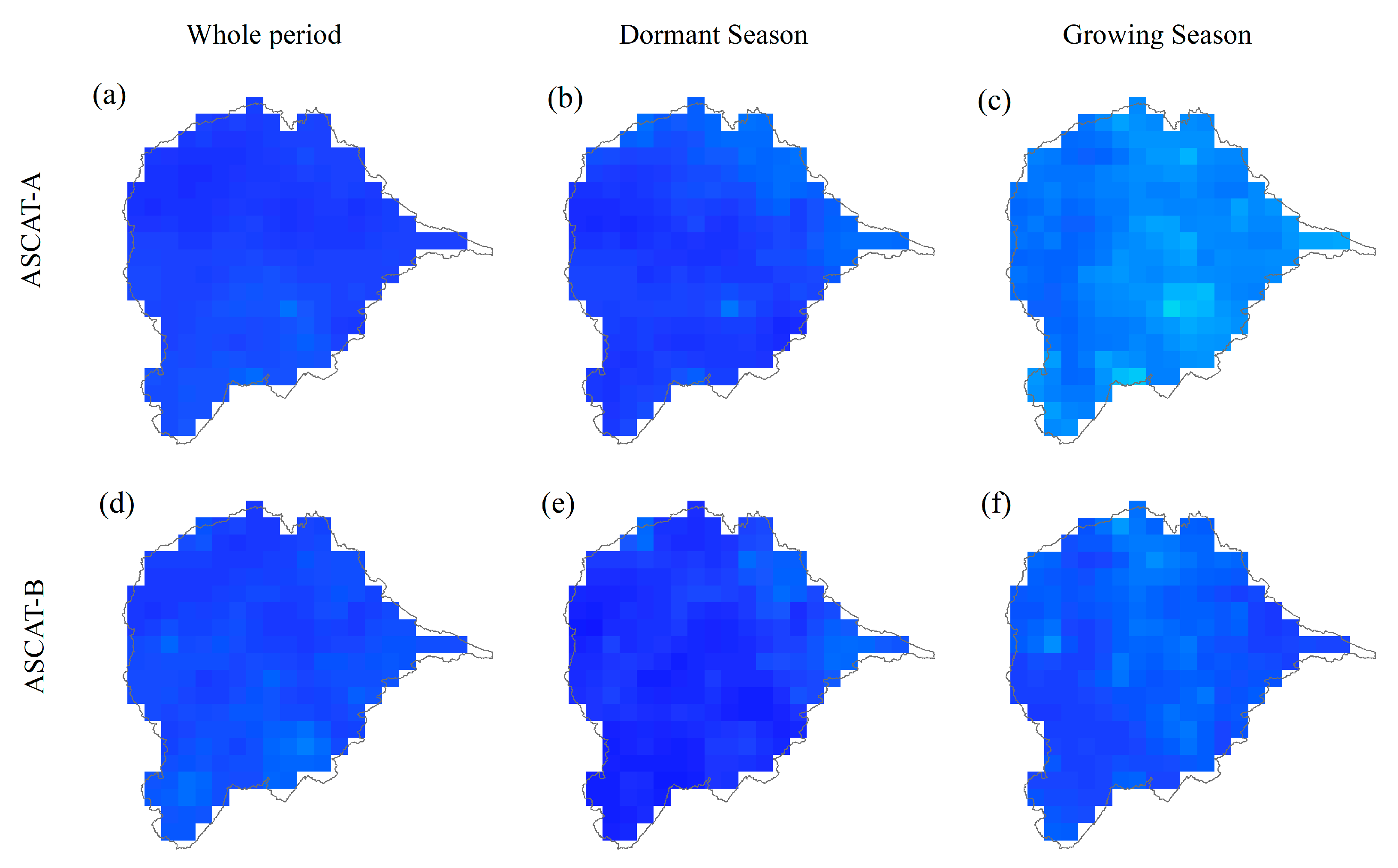
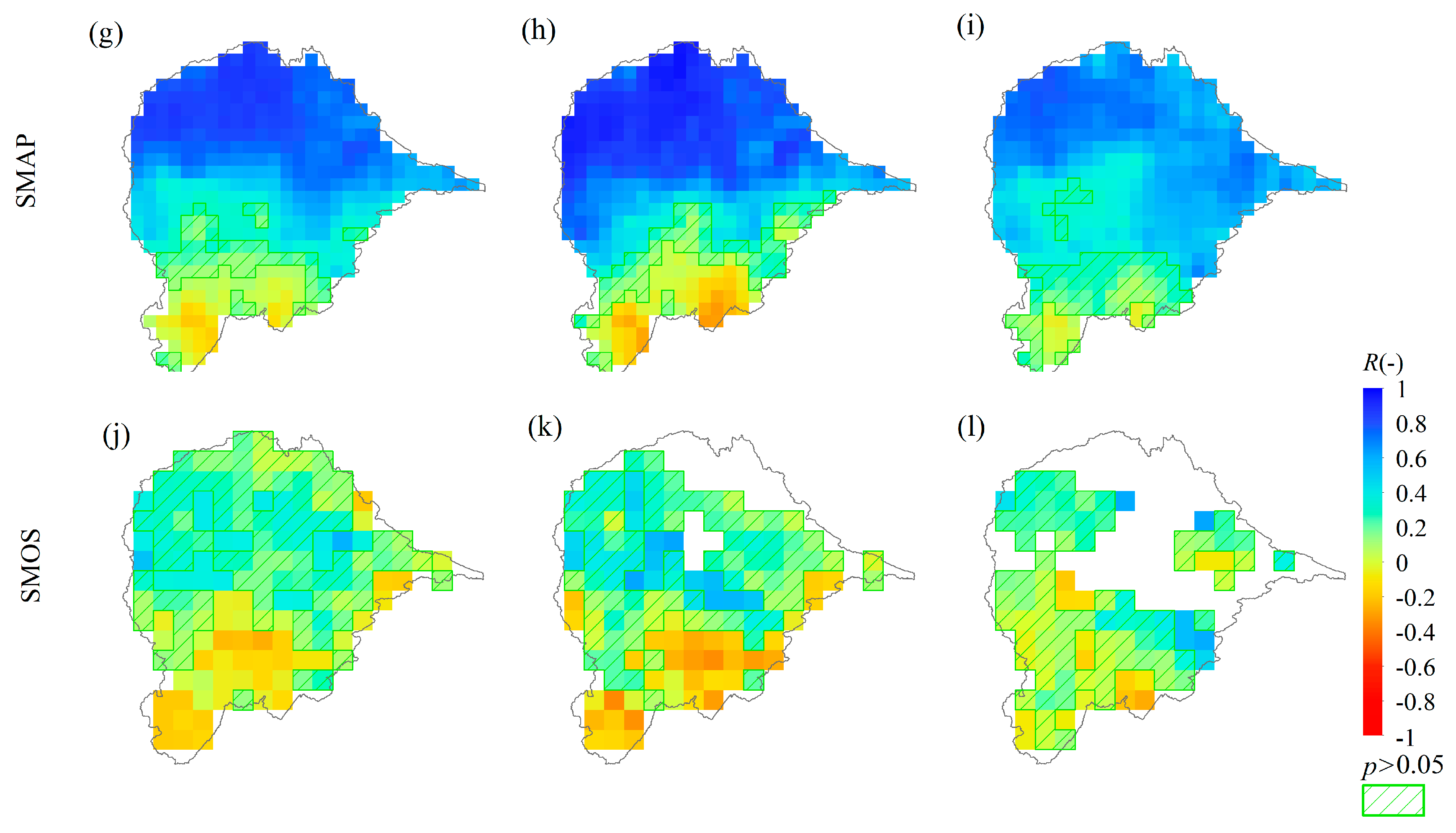
4.3.2. Spatial Distributions

In this section, ${\omega }_{SSM}^{RS}$ and ${\omega }_{SWI}^{RS}$ values derived from remotely sensed products are compared with saturation degree simulated by DDRM (ω^DDRM) at grid scale.

Table 5. Statistics of grid correlation-coefficient values between saturation degree values acquired from each remotely sensed product (${\omega }_{SSM}^{RS}$ and ${\omega }_{SWI}^{RS}$) with those from DDRM (ω^DDRM) during different periods of 2010–2016 (the whole period, the dormant seasons and the growing seasons). N represents sample sizes used for comparisons. R values are shown in brackets when p > 0.05.

Satellite	Period	R(${\mathit{\omega }}_{\mathit{S}\mathit{S}\mathit{M}}^{\mathit{R}\mathit{S}}$,ωDDRM)/N			R(${\mathit{\omega }}_{\mathit{S}\mathit{W}\mathit{I}}^{\mathit{R}\mathit{S}}$,ωDDRM)/N
		Highest	Mean	Lowest	Highest	Mean	Lowest
ASCAT-A	Whole	0.71/1912	0.61/1913	0.39/1887	0.88/1913	0.81/1913	0.67/1885
	Dormant	0.62/1112	0.45/1105	0.27/1106	0.89/1110	0.79/1105	0.65/1105
	Growing	0.57/802	0.43/802	0.31/802	0.71/802	0.61/802	0.36/802
ASCAT-B	Whole	0.75/1006	0.60/1007	0.41/990	0.89/1007	0.83/1007	0.68/990
	Dormant	0.65/542	0.48/549	0.28/547	0.93/544	0.83/549	0.66/549
	Growing	0.55/459	0.45/459	0.34/459	0.89/459	0.83/459	0.68/459
SMAP	Whole	0.66/305	0.33/305	−0.35/303	0.87/305	0.38/305	−0.48/303
	Dormant	0.73/162	0.35/160	−0.30/160	0.96/162	0.42/160	−0.63/160
	Growing	0.64/145	0.34/143	−0.28/138	0.76/144	0.37/143	−0.32/138
SMOS	Whole	0.36/280	(0.08)/358	(−0.12)/434	0.54/281	(0.13)/348	−0.27/445
	Dormant	0.34/114	(0.06)/150	−0.24/226	0.56/114	(0.13)/151	−0.28/223
	Growing	0.30/119	(0.06)/147	−0.25/215	0.40/119	(0.07)/148	−0.36/215

presents the statistics of correlation-coefficient values between gridded saturation degree values from satellites with those from DDRM during the whole period, the dormant season and the growing season. For all satellites, the differences between the remotely sensed soil moisture and the model-simulated soil moisture tend to be smaller for ${\omega }_{SWI}^{RS}$. This is because SWI is more likely to represent the profile soil moisture, which is more comparable to the model-simulated soil moisture, but SSM represents the soil moisture for the depth of about 0–5 cm of the soil layer. For each remotely sensed product, the regional influences on R with ω^DDRM are similar for ${\omega }_{SSM}^{RS}$ and ${\omega }_{SWI}^{RS}$ values, thus, for the sake of brevity, only parts of ${\omega }_{SWI}^{RS}$ data are chosen to show spatial distributions of comparisons with ω^DDRM , as presented in Figure 12, in which the grids where p-value is above 0.05 are highlighted by green lines. As Table 5 and Figure 12 show, correlation-coefficient values between ${\omega }_{SSM}^{RS}$ and ω^DDRM, as well as those between ${\omega }_{SWI}^{RS}$ and ω^DDRM, are higher in dormant seasons than those in growing seasons.

This is different from results of Peng et al., who found that ASCAT and SMOS products have small variations over different seasons in terms of R and RMSD values with ground measurements [59]. Thus, the seasonal difference of R is probably due to the relatively poor performance of DDRM in dormant seasons than in growing seasons, so ω^DDRM tends to be less reliable during dormant seasons.

Figure 13 depicts, for each satellite product and for three kinds of concerned grids (grids with the highest, mean and the lowest correlation-coefficient values between ${\omega }_{SWI}^{RS}$ and ω^DDRM), three soil moisture time series, i.e., the remotely sensed soil moisture (${\omega }_{SWI}^{RS}$ and ${\omega }_{SWI}^{RS}$) and the corresponding ω^DDRM over the whole year 2016. Similar to Figure 11, this figure indicates that grids with ${\omega }_{SWI}^{RS}$ time series of high fluctuant intensity show lower correlation-coefficient values with ω^DDRM than those with ${\omega }_{SWI}^{RS}$ time series of low fluctuant intensity. For all remotely sensed soil moisture, the range of ${\omega }_{SWI}^{RS}$ values tends to be narrower than that of ω^DDRM values, similar to the results of [26]. This may related to the simple criterion used in the study to select the same T value applied to different remotely sensed products.

Two ASCAT products (ASCAT-A and ASCAT-B) show similar patterns in terms of R with the model-simulated soil moisture across Qujiang catchment. The average correlation-coefficient values of ${\omega }_{SSM}^{ASCSAT}$ and ω^DDRM range from 0.43 to 0.61, and those of ${\omega }_{SWI}^{ASCSAT}$ and ω^DDRM range from 0.61 to 0.83. Compared to other satellite products, ${\omega }_{SWI}^{ASCSAT}$ show the highest correlation-coefficients with ω^DDRM. As shown in Figure 13, time series of soil moisture values from both ASCAT products also fit quiet well with soil moisture values simulated by DDRM in three specific grids, which is consistent with the results of catchment-wide averages (Figure 11). Moreover, the standard-deviation values of correlation coefficient are notably low for ASCAT products, ranging from 0.04 to 0.08, which means the agreement between ASCAT products and DDRM soil moisture does not notably change with land use groups and altitudes. This result is in agreement with Peng et al. [59], who show different land use groups have similar performance in terms of R for ASCAT products over southwest China. This is not always the case in previous studies [42,62,63], which showed a strong connection between the quality of ASCAT retrieves and vegetation density.

The reason for the discrepancy in southwest area of China may be that different land-use types do not represent different vegetation densities in the study area. According to Figure 2, the Normalized Difference Vegetation Index (NDVI) over the study area only changes with seasons, but not changes obviously with land uses. On the other hand, the discrepancy may be due to the small variation of the DDRM soil moisture with different land uses, since DDRM failed to consider the influence of land uses on soil moisture estimations. Thus, the results of the comparison between ASCAT products and the model-simulated soil moisture are reasonable.

SMAP product is with relatively higher standard deviation values than ASCAT products, from 0.17 to 0.44. The highest correlation-coefficient values of ${\omega }_{SWI}^{SMAP}$ and ω^DDRM are 0.87, 0.96 and 0.76 for the whole period, the dormant seasons and the growing seasons, respectively, while the lowest values are −0.48, −0.63, −0.32. Figure 12 presents that the correlation-coefficient values of ${\omega }_{SWI}^{SMAP}$ and ω^DDRM are high in higher grids with land use group of forest, at around 0.75, while lower grids with land use group of dry and cultivated land show poor correlations, where correlation-coefficient values are around or below 0. This difference is especially notable in dormant seasons. According to Figure 11 and Figure 13, the poor correlations in the flat regions may partly due to the fact that SMAP soil moisture is drying faster than the model-simulated soil moisture after rainfalls because of high evaporation rates of dry and cultivated land in flat regions of Qujiang catchment. This result is similar to the findings of Shellito et al. (2016), who found SMAP soil moisture differs from in situ observed soil moisture in drying rate [64].

Both ${\omega }_{SSM}^{SMOS}$ and ${\omega }_{SWI}^{SMOS}$ show poor correlations with ω^DDRM across the Qujiang catchment. The grids with the highest correlation-coefficient values of SMOS soil moisture and the model-simulated soil moisture, which are 0.36 for ${\omega }_{SSM}^{SMOS}$ and 0.54 for ${\omega }_{SWI}^{SMOS}$ during the whole period, are situated at high altitudes. For this product, the p-value exceeds 0.05 for more than half number of the total grids, most of which are situated in lower areas. This is largely due to the severe effects of radio frequency interference (RFI) over southwestern China. This result is in agreement with findings of previous studies [34], which found large errors occurred for SMOS soil moisture data when they were compared with ground measurements over southwestern China. Another reason to consider is the low temporal resolution for each grid, where available data of soil moisture from SMOS are considerably less than that of the SMAP and ASCAT products.

5. Conclusions

This study evaluates the consistency between daily soil moisture acquired from four remotely sensed soil moisture products, including ASCAT-A, ASCAT-B, SMAP and SMOS products, and two hydrological models, including XAJ model and DDRM across the Qujiang catchment in southwest China during 2010–2016. It compares: (i) the spatial distributions of daily remotely sensed and model-simulated soil moisture and (ii) the daily catchment-averaged soil moisture from different sources across the Qujiang catchment. Since surface soil moisture SSM acquired from satellites and the soil moisture storage simulated by hydrological models represent different soil layers, the profile soil moisture, which is represented by SWI and is rather comparable to the depth of the model-simulated soil moisture, is estimated by the exponential filter to address this mismatch. The same T value is used to calculate SWI from different sensors to be compared with different model-simulated soil moisture. On the other hand, since the discrepancies in the way the remotely sensed and the model-simulated soil moisture are obtained, they typically exhibit very different mean values and variability. These discrepancies pose a severe obstacle to exploiting the useful information contained in satellite retrievals through data comparisons or assimilation. In the study, soil moisture datasets from all sources are rescaled between 0 and 1 in their long-term periods for error removals.

The following conclusions are drawn:

• Soil moisture simulated by the XAJ model and DDRM tends to represent soil moisture of similar soil depth, and each satellite soil moisture product shows similar correlations when compared with soil moisture from XAJ model or DDRM.
• The quantitative assessments of the different results between SSM and SWI values in this study indicate that SWI is more likely to reveal the change of XAJ and DDRM model-simulated soil moisture. The characteristic time length $T$ of the exponential filter that maximizes the overall correlation coefficient R between catchment-wide remotely sensed SWI averages and model-simulated averages equals to 20 days in this study. Better results could be acquired for SWI when optimal T values are applied to sensors measuring different soil depth to be compared to different model-simulated soil moistures, since optimal T value is affected by a range of environmental factors, such as soil depth, soil texture, and climatic conditions and other soil or climatic variables.
• SMAP soil moisture values are higher than ASCAT and SMOS soil moisture values across the Qujiang catchment. ASCAT soil moisture products (ASCAT-A and ASCAT-B) show the highest agreement with the model-simulated soil moisture at both high spatial resolutions (i.e., grids) and large spatial scales (i.e., the whole catchment) for different seasons, followed by SMAP product. However, SMOS soil moisture product always shows low correlations with the model-simulated soil moisture.
• Correlation-coefficient values between the remotely sensed and the model-simulated soil moisture are likely influenced by different land use types. Different remotely sensed soil moisture products have different patterns in terms of correlation-coefficient values with model-simulated soil moisture in alpine (forest land) and flat regions (dry and cultivated land). The regional differences of correlations between the ASCAT products and model-simulated soil moisture are generally smaller than the differences between the SMAP product and model-simulated soil moisture. ASCAT products show similar correlations with the model-simulated soil moisture in either alpine or flat regions of the Qujiang catchment, while the SMAP product shows high correlation-coefficient values in the alpine regions, but dramatically lower figures in the flat regions, especially in dormant seasons. The difference may be due to the different retrieval algorithms between active and passive sensors.
• Although all remotely sensed soil moisture products agree better with the model-simulated soil moisture in dormant seasons, the consistency during these seasons might not be reliable because of slight changes of low soil moisture values and poor performances of streamflow simulations for models during these seasons.

Overall, the results are encouraging, and modelers can consider using these remotely sensed soil moisture data for model validation, calibration, or input assimilation, but careful consideration is also required when using soil moisture information acquired from indirect ways in ground measurement-sparse areas. The same T value used may lead to uncertainty, since no clear criteria are defined to maintain the T value as a general value. In fact, the different representativeness of soil layers makes how to propagate remotely sensed surface soil moisture information to the root-zone layer a well-recognized challenge. More sophisticated criteria are needed to be used to select suitable T values for different sensors and models in the further study. Besides, the rescaling method used in the study has its limitations as well, since when remotely sensed soil moisture products are compared with the model-simulated soil moisture, non-linearity appears. Thus, non-linear rescaling methods, i.e., Variance Matching (VM) or Cumulative Distribution Function (CDF), are needed to be considered for bias removal in the future.

Considering that the currently employed objective function NSE focuses more on high flows than on low flows thus leading to the worse performance of streamflow simulation for hydrological models during dormant seasons, further study could choose other objective functions that are more capable for simulating soil moisture during low-flow periods. In the study, both models use Blaney-Criddle method for PET estimations. Since this methodology has its limitations and can result to significant over or under estimations of the PET, more sophisticated estimation methods for the PET can be used when simulating soil moisture by hydrological models. Besides, more satellite soil moisture products and longer time series of soil moisture can be considered in the future research.

References

1. Wagner, W.; Scipal, K.; Pathe, C.; Gerten, D.; Lucht, W.; Rudolf, B. Evaluation of the agreement between the first global remotely sensed soil moisture data with model and precipitation data. J. Geophys. Res. Atmos. 2003, 108, 4611. [Google Scholar] [CrossRef]
2. Tayfur, G.; Brocca, L. Fuzzy logic for rainfall-runoff modelling considering soil moisture. Water Resour. Manag. 2015, 29, 3519–3533. [Google Scholar] [CrossRef]
3. Srivastava, P.K. Satellite soil moisture: Review of theory and applications in water resources. Water Resour. Manag. 2017, 31, 3161–3176. [Google Scholar] [CrossRef]
4. Walker, J.P. Estimating Soil Moisture Profile Dynamics from Near-Surface Soil Moisture Measurements and Standard Meteorological Data. Ph.D. Thesis, University of Newcastle, Callaghan, Australia, 1999. [Google Scholar]
5. Pal, M.; Maity, R.; Dey, S. Statistical Modelling of vertical soil moisture profile: Coupling of memory and forcing. Water Resour. Manag. 2016, 30, 1973–1986. [Google Scholar] [CrossRef]
6. Liu, Y.Y.; Parinussa, R.; Dorigo, W.A.; De Jeu, R.A.; Wagner, W.; Van Dijk, A.; McCabe, M.F.; Evans, J. Developing an improved soil moisture dataset by blending passive and active microwave satellite-based retrievals. Hydrol. Earth Syst. Sci. 2011, 15, 425–436. [Google Scholar] [CrossRef] [Green Version]
7. Bartalis, Z.; Wagner, W.; Naeimi, V.; Hasenauer, S.; Scipal, K.; Bonekamp, H.; Figa, J.; Anderson, C. Initial soil moisture retrievals from the METOP-A Advanced Scatterometer (ASCAT). Geophys. Res. Lett. 2007, 34, L20401. [Google Scholar] [CrossRef]
8. Kerr, Y.H.; Al-Yaari, A.; Rodriguez-Fernandez, N.; Parrens, M.; Molero, B.; Leroux, D.; Birchera, S.; Mahmoodia, A.; Mialona, A.; Richaumea, P.; et al. Overview of SMOS performance in terms of global soil moisture monitoring after six years in operation. Remote Sens. Environ. 2016, 180, 40–63. [Google Scholar] [CrossRef]
9. Entekhabi, D.; Njoku, E.G.; O’Neill, P.E.; Kellogg, K.H.; Crow, W.T.; Edelstein, W.N.; Entin, J.K.; Goodman, S.D.; Jackson, T.J.; Johnson, J. The soil moisture active passive (SMAP) mission. Proc. IEEE 2010, 98, 704–716. [Google Scholar] [CrossRef]
10. Alexakis, D.; Mexis, F.-D.; Vozinaki, A.-E.; Daliakopoulos, I.; Tsanis, I. Soil moisture content estimation based on Sentinel-1 and auxiliary earth observation products. A hydrological approach. Sensors 2017, 17, 1455. [Google Scholar] [CrossRef] [PubMed]
11. Xing, C.; Chen, N.; Zhang, X.; Gong, J. A machine learning based reconstruction method for satellite remote sensing of soil moisture images with in situ observations. Remote Sens. 2017, 9, 484. [Google Scholar] [CrossRef]
12. Srivastava, P.K.; Han, D.; Rico-Ramirez, M.A.; Al-Shrafany, D.; Islam, T. Data fusion techniques for improving soil moisture deficit using SMOS satellite and WRF-NOAH land surface model. Water Resour. Manag. 2013, 27, 5069–5087. [Google Scholar] [CrossRef]
13. Wanders, N.; Bierkens, M.F.; de Jong, S.M.; de Roo, A.; Karssenberg, D. The benefits of using remotely sensed soil moisture in parameter identification of large-scale hydrological models. Water Resour. Res. 2014, 50, 6874–6891. [Google Scholar] [CrossRef]
14. Silvestro, F.; Gabellani, S.; Rudari, R.; Delogu, F.; Laiolo, P.; Boni, G. Uncertainty reduction and parameter estimation of a distributed hydrological model with ground and remote-sensing data. Hydrol. Earth Syst. Sci. 2015, 19, 1727–1751. [Google Scholar] [CrossRef]
15. Zhao, R.J. The Xinanjiang model applied in China. J. Hydrol. 1992, 135, 371–381. [Google Scholar] [CrossRef]
16. Beven, K. TOPMODEL: A critique. Hydrol. Process. 1997, 11, 1069–1085. [Google Scholar] [CrossRef]
17. Xiong, L.; Guo, S.L.; Tian, X.R. DEM-based distributed hydrological model and its application. Adv. Water Sci. 2004, 15, 517–520. (In Chinese) [Google Scholar]
18. Jackson, T.J.; Bindlish, R.; Cosh, M.H.; Zhao, T.; Starks, P.J.; Bosch, D.D.; Seyfried, M.; Moran, M.S.; Goodrich, D.C.; Kerr, Y.H. Validation of soil moisture and ocean salinity (SMOS) soil moisture over watershed networks in the US. IEEE Trans. Geosci. Remote Sens. 2012, 50, 1530–1543. [Google Scholar] [CrossRef] [Green Version]
19. Yee, M.S.; Walker, J.P.; Monerris, A.; Rüdiger, C.; Jackson, T.J. On the identification of representative in situ soil moisture monitoring stations for the validation of SMAP soil moisture products in Australia. J. Hydrol. 2016, 537, 367–381. [Google Scholar] [CrossRef]
20. Rüdiger, C.; Calvet, J.C.; Gruhier, C.; Holmes, T.R.; De Jeu, R.A.; Wagner, W. An intercomparison of ERS-Scat and AMSR-E soil moisture observations with model simulations over France. J. Hydrometeorol. 2009, 10, 431–447. [Google Scholar] [CrossRef]
21. Albergel, C.; Rüdiger, C.; Carrer, D.; Calvet, J.C.; Fritz, N.; Naeimi, V.; Bartalis, Z.; Hasenauer, S. An evaluation of ASCAT surface soil moisture products with in-situ observations in Southwestern France. Hydrol. Earth Syst. Sci. 2009, 13, 115–124. [Google Scholar] [CrossRef]
22. Lacava, T.; Matgen, P.; Brocca, L.; Bittelli, M.; Pergola, N.; Moramarco, T.; Tramutoli, V. A first assessment of the SMOS soil moisture product with in situ and modeled data in Italy and Luxembourg. IEEE Trans. Geosci. Remote Sens. 2012, 50, 1612–1622. [Google Scholar] [CrossRef]
23. Dall’Amico, J.T.; Schlenz, F.; Loew, A.; Mauser, W. First results of SMOS soil moisture validation in the upper Danube catchment. IEEE Trans. Geosci. Remote Sens. 2012, 50, 1507–1516. [Google Scholar] [CrossRef]
24. Pan, M.; Cai, X.; Chaney, N.W.; Entekhabi, D.; Wood, E.F. An initial assessment of SMAP soil moisture retrievals using high-resolution model simulations and in situ observations. Geophys. Res. Lett. 2016, 43, 9662–9668. [Google Scholar] [CrossRef]
25. Reichle, R.H.; Koster, R.D.; Dong, J.; Berg, A.A. Global soil moisture from satellite observations, land surface models, and ground data: Implications for data assimilation. J. Hydrometeorol. 2004, 5, 430–442. [Google Scholar] [CrossRef]
26. Brocca, L.; Melone, F.; Moramarco, T.; Wagner, W.; Hasenauer, S. ASCAT soil wetness index validation through in situ and modeled soil moisture data in central Italy. Remote Sens. Environ. 2010, 114, 2745–2755. [Google Scholar] [CrossRef]
27. Albergel, C.; De Rosnay, P.; Gruhier, C.; Muñoz-Sabater, J.; Hasenauer, S.; Isaksen, L.; Kerr, Y.; Wagner, W. Evaluation of remotely sensed and modelled soil moisture products using global ground-based in situ observations. Remote Sens. Environ. 2012, 118, 215–226. [Google Scholar] [CrossRef]
28. Al-Yaari, A.; Wigneron, J.P.; Kerr, Y.; Rodriguez-Fernandez, N.; O’Neill, P.E.; Jackson, T.J.; De Lannoy, G.J.M.; Al Bitar, A.; Mialon, A.; Richaume, P.; et al. Evaluating soil moisture retrievals from ESA’s SMOS and NASA’s SMAP brightness temperature datasets. Remote Sens. Environ. 2017, 193, 257–273. [Google Scholar] [CrossRef]
29. Parajka, J.; Naeimi, V.; Blöschl, G.; Komma, J. Matching ERS scatterometer based soil moisture patterns with simulations of a conceptual dual layer hydrologic model over Austria. Hydrol. Earth Syst. Sci. 2009, 13, 259–271. [Google Scholar] [CrossRef]
30. Grillakis, M.G.; Koutroulis, A.G.; Komma, J.; Tsanis, I.K.; Wagner, W.; Blöschl, G. Initial soil moisture effects on flash flood generation—A comparison between basins of contrasting hydro-climatic conditions. J. Hydrol. 2016. [Google Scholar] [CrossRef]
31. Alvarez-Garreton, C.; Ryu, D.; Western, A.W.; Crow, W.T.; Su, C.H.; Robertson, D.R. Dual assimilation of satellite soil moisture to improve streamflow prediction in data-scarce catchments. Water Resour. Res. 2016, 52, 5357–5375. [Google Scholar] [CrossRef]
32. Tian, S.; Tregoning, P.; Renzullo, L.J.; van Dijk, A.I.; Walker, J.P.; Pauwels, V.; Allgeyer, S. Improved water balance component estimates through joint assimilation of GRACE water storage and SMOS soil moisture retrievals. Water Resour. Res. 2017, 53, 1820–1840. [Google Scholar] [CrossRef]
33. Sinclair, S.; Pegram, G.G.S. A comparison of ASCAT and modelled soil moisture over South Africa, using TOPKAPI in land surface mode. Hydrol. Earth Syst. Sci. 2010, 14, 613–626. [Google Scholar] [CrossRef]
34. Hain, C.R.; Crow, W.T.; Mecikalski, J.R.; Anderson, M.C.; Holmes, T. An intercomparison of available soil moisture estimates from thermal infrared and passive microwave remote sensing and land surface modeling. J. Geophys. Res. Atmos. 2011, 116. [Google Scholar] [CrossRef]
35. Hu, Z.; Chen, Y.; Yao, L.; Wei, C.; Li, C. Optimal allocation of regional water resources: From a perspective of equity–efficiency tradeoff. Resour. Conserv. Recycl. 2016, 109, 102–113. [Google Scholar] [CrossRef]
36. Nachtergaele, F.O.; van Velthuizen, H.; Verelst, L.; Batjes, N.H.; Dijkshoorn, J.A.; van Engelen, V.W.P.; Fischer, G.; Jone, A.; Montanarella, L.; Petri, M.; et al. Harmonized World Soil Database (Version 1.0); Food and Agriculture Organization of the UN (FAO); International Inst. for Applied Systems Analysis (IIASA); ISRIC-World Soil Information; Inst. of Soil Science-Chinese Academic of Sciences (ISS-CAS); EC-Joint Research Centre (JRC): Laxenburg, Austria, 2008. [Google Scholar]
37. Saxton, K.E.; Rawls, W.J. Soil water characteristic estimates by texture and organic matter for hydrologic solutions. Soil Sci. Soc. Am. J. 2006, 70, 1569–1578. [Google Scholar] [CrossRef]
38. Hargreaves, G.H.; Samani, Z.A. Estimating potential evapotranspiration. J. Irrig. Drain. Div. 1982, 108, 225–230. [Google Scholar]
39. Tomczak, M. Spatial interpolation and its uncertainty using automated anisotropic inverse distance weighting (IDW)-cross-validation/jackknife approach. J. Geogr. Inf. Decis. Anal. 1998, 2, 18–30. [Google Scholar]
40. Figa-Saldaña, J.; Wilson, J.J.; Attema, E.; Gelsthorpe, R.; Drinkwater, M.; Stoffelen, A. The advanced scatterometer (ASCAT) on the meteorological operational (MetOp) platform: A follow on for European wind scatterometers. Can. J. Remote Sens. 2002, 28, 404–412. [Google Scholar] [CrossRef]
41. Anderson, C.; Figa, J.; Bonekamp, H.; Wilson, J.; Verspeek, J.; Stoffelen, A.; Portabella, M. Validation of backscatter measurements from the advanced scatterometer on MetOp-A. J. Atmos. Ocean. Technol. 2011, 29, 77–88. [Google Scholar] [CrossRef]
42. Wagner, W.; Hahn, S.; Kidd, R.; Melzer, T.; Bartalis, Z.; Hasenauer, S.; Figa-Saldaña, J.; de Rosnay, P.; Jann, A.; Schneider, S. The ASCAT soil moisture product: A review of its specifications, validation results, and emerging applications. Meteorol. Z. 2013, 22, 5–33. [Google Scholar] [CrossRef]
43. O’Neill, P.E.; Chan, S.; Njoku, E.G.; Jackson, T.; Bindlish, R. SMAP Enhanced L3 Radiometer Global Daily 9 km EASE-Grid Soil Moisture, Version 1. [Indicate Subset Used]. Boulder, Colorado USA. NASA National Snow and Ice Data Center Distributed Active Archive Center. 2016. Available online: http://dx.doi.org/10.5067/ZRO7EXJ8O3XI (accessed on 27 May 2017).
44. Zeng, J.; Chen, K.S.; Bi, H.; Chen, Q. A preliminary evaluation of the SMAP radiometer soil moisture product over United States and Europe using ground-based measurements. IEEE Trans. Geosci. Remote Sens. 2016, 54, 4929–4940. [Google Scholar] [CrossRef]
45. Kerr, Y.H.; Waldteufel, P.; Richaume, P.; Wigneron, J.P.; Ferrazzoli, P.; Mahmoodi, A.; Al Bitar, A.; Cabot, F.; Gruhier, C.; Juglea, S.E. The SMOS soil moisture retrieval algorithm. IEEE Trans. Geosci. Remote Sens. 2012, 50, 1384–1403. [Google Scholar] [CrossRef]
46. Wigneron, J.P.; Kerr, Y.; Waldteufel, P.; Saleh, K.; Escorihuela, M.J.; Richaume, P.; Ferrazzoll, P.; de Rosnay, P.; Gurney, R.; Calvet, J.C.; et al. L-band microwave emission of the biosphere (L-MEB) model: Description and calibration against experimental data sets over crop fields. Remote Sens. Environ. 2007, 107, 639–655. [Google Scholar] [CrossRef]
47. Al-Yaari, A.; Wigneron, J.P.; Ducharne, A.; Kerr, Y.H.; Wagner, W.; De Lannoy, G.; Reichle, R.; Al Bitar, A.; Dorigo, W.; Richaume, P.; et al. Global-scale comparison of passive (SMOS) and active (ASCAT) satellite based microwave soil moisture retrievals with soil moisture simulations (MERRA-Land). Remote Sens. Environ. 2014, 152, 614–626. [Google Scholar] [CrossRef] [Green Version]
48. Wagner, W.; Lemoine, G.; Rott, H. A Method for Estimating Soil Moisture from ERS Scatterometer and Soil Data. Remote Sens. Environ. 1999, 70, 191–207. [Google Scholar] [CrossRef]
49. Hu, C.; Guo, S.L.; Xiong, L.; Peng, D. A modified Xinanjiang model and its application in northern China. Hydrol. Res. 2005, 36, 175–192. [Google Scholar]
50. Duan, Q.; Sorooshian, S.; Gupta, V. Effective and efficient global optimization for conceptual rainfall-runoff models. Water Resour. Res. 1992, 28, 1015–1031. [Google Scholar] [CrossRef]
51. Xiong, L.; Guo, S.L.; Chen, H.; Lin, K.R.; Cheng, J.-Q. Application of the hydro-network model in the distributed hydrological modeling. J. China Hydrol. 2007, 2, 005. (In Chinese) [Google Scholar]
52. Xiong, L.; Guo, S.L. Distributed Watershed Hydrological Model; China Water Power Press: Beijing, China, 2004. [Google Scholar]
53. Long, H.-F.; Xiong, L.; Wan, M. Application of DEM-based distributed hydrological model in Qingjiang river basin. Resour. Environ. Yangtze Basin 2012, 21, 71–78. (In Chinese) [Google Scholar]
54. Jones, R. Algorithms for using a DEM for mapping catchment areas of stream sediment samples. Comput. Geosci. 2002, 28, 1051–1060. [Google Scholar] [CrossRef]
55. Massari, C.; Brocca, L.; Barbetta, S.; Papathanasiou, C.; Mimikou, M.; Moramarco, T. Using globally available soil moisture indicators for flood modelling in Mediterranean catchments. Hydrol. Earth Syst. Sci. 2014, 18, 839–853. [Google Scholar] [CrossRef] [Green Version]
56. Cho, E.; Choi, M.; Wagner, W. An assessment of remotely sensed surface and root zone soil moisture through active and passive sensors in northeast Asia. Remote Sens. Environ. 2015, 160, 166–179. [Google Scholar] [CrossRef]
57. Albergel, C.; Rüdiger, C.; Pellarin, T.; Calvet, J.C.; Fritz, N.; Froissard, F.; Suquia, D.; Petitpa, A.; Piguet, B.; Martin, E. From near-surface to root-zone soil moisture using an exponential filter: An assessment of the method based on in-situ observations and model simulations. Hydrol. Earth Syst. Sci. 2008, 12, 1323–1337. [Google Scholar] [CrossRef]
58. Sánchez-Ruiz, S.; Piles, M.; Sánchez, N.; Martínez-Fernández, J.; Vall-llossera, M.; Camps, A. Combining SMOS with visible and near/shortwave/thermal infrared satellite data for high resolution soil moisture estimates. J. Hydrol. 2014, 516, 273–283. [Google Scholar] [CrossRef]
59. Peng, J.; Niesel, J.; Loew, A.; Zhang, S.; Wang, J. Evaluation of satellite and reanalysis soil moisture products over Southwest China using ground-based measurements. Remote Sens. 2015, 7, 15729–15747. [Google Scholar] [CrossRef]
60. Pauwels, V.R.; Hoeben, R.; Verhoest, N.E.; De Troch, F.P. The importance of the spatial patterns of remotely sensed soil moisture in the improvement of discharge predictions for small-scale basins through data assimilation. J. Hydrol. 2001, 251, 88–102. [Google Scholar] [CrossRef]
61. Kim, H.; Parinussa, R.; Konings, A.G.; Wagner, W.; Cosh, M.H.; Lakshmi, V.; Zohaib, M.; Choi, M. Global-scale assessment and combination of SMAP with ASCAT (active) and AMSR2 (passive) soil moisture products. Remote Sens. Environ. 2017, 204, 260–275. [Google Scholar] [CrossRef]
62. Parinussa, R.; Meesters, A.G.; Liu, Y.Y.; Dorigo, W.; Wagner, W.; De Jeu, R.A.M. Error estimates for near-real-time satellite soil moisture as derived from the land parameter retrieval model. IEEE Geosci. Remote Sens. Lett. 2011, 8, 770–783. [Google Scholar] [CrossRef]
63. Brocca, L.; Hasenauer, S.; Lacava, T.; Melone, F.; Moramarco, T.; Wagner, W.; Dorigo, W.; Matgen, P.; Martínez-Fernández, J.; Llorens, P.; et al. Soil moisture estimation through ASCAT and AMSR-E sensors: An intercomparison and validation study across Europe. Remote Sens. Environ. 2011, 115, 3390–3408. [Google Scholar] [CrossRef]
64. Shellito, P.J.; Small, E.E.; Colliander, A.; Bindlish, R.; Cosh, M.H.; Berg, A.A.; Bosch, D.D.; Caldwell, T.G.; Goodrich, D.C.; McNairn, H. SMAP soil moisture drying more rapid than observed in situ following rainfall events. Geophys. Res. Lett. 2016, 43, 8068–8075. [Google Scholar] [CrossRef]
Figure 1. Topography (b) and land use (c) in 2010 of the Qujiang catchment in China (a): (a) the location of the Qujiang catchment (blue-shaded); (b) river networks (blue lines) and sub-catchments (circled by red lines), as well as meteorological stations (blue dots) and a hydrological station (red triangle) at the outlet of the Qujiang catchment.
Water 10 00291 g001
Figure 2. Normalized Difference Vegetation Index (NDVI) in different months of the year 2016 for the Qujiang catchment.
Water 10 00291 g002
Figure 3. Flow chart for the Xinanjing model. This model is driven by precipitation and potential evapotranspiration, and the main outputs are actual evapotranspiration, total outflow, and soil moisture content. It generates runoff from both pervious area (FR) and impervious areas (1-FR). This paper choses areal mean tension water storage (W) (purple-shaded) as the XAJ model-simulated soil moisture content. The symbols in square brackets such as [K] represent the model parameters, while the symbols in brackets such as (EW) represent state variables.
Water 10 00291 g003
Figure 4. Discretization of catchment into sub-catchments and grids, and also delineation of streamflow routing (represented by blue lines) in the DEM-based rainfall-runoff model (DDRM). d, e, f represent the outlet of sub-catchments 1 (grey-shaded), 2 (light blue-shaded) and 3 (yellow-shaded), respectively.
Water 10 00291 g004
Figure 5. Hydrological processes involved in a grid where there is no excess rainfall generation (a) and a grid where there is the excess rainfall generation (b), and streamflow movement across both kinds of grids in DDRM.
Water 10 00291 g005
Figure 6. Averaged surface soil moisture contents ( θ S S M R S ) (top panel) and soil wetness index ( θ S W I R S ) (bottom panel) over the whole period of the different remotely sensed products.
Water 10 00291 g006
Figure 7. Soil wetness index ( θ S W I R S ) given in m3 m−3 estimated based on θ S S M R S acquired from four remotely sensed soil moisture products on the fourth of May (left column), the thirteenth of June (middle column) and the twenty-seventh of June (right column) during a water-rising stage of 2016.
Water 10 00291 g007aWater 10 00291 g007b
Figure 8. Observed daily discharge (black lines) for the Qujiang catchment compared with simulated discharge from XAJ model (red lines) and DDRM (blue line) and corresponding precipitation (green-shaded) during the flood period (6.15–8.15) of 2016 (a). (b) Observed and modelled daily flow duration curve during the whole period of 2010–2016.
Water 10 00291 g008
Figure 9. Overall averages of DDRM model-simulated soil moisture storage depth over the whole period (a), and DDRM model-simulated soil moisture storage depth on the fourth of May (b), the thirteenth of June (c) and the twenty-seventh of June (d) during a water-rising stage of 2016. The resolution is 1 km.
Water 10 00291 g009
Figure 10. Correlations between catchment-averaged ω S S M R S from different satellite products. (a) between ASCAT-A and ASCAT-B; (b) between ASCAT-A and SMAP; (c) between ASCAT-A and SMOS; (d) between ASCAT-B and SMAP; (e) between ASCAT-B and SMOS; (f) between SMAP and SMOS.
Water 10 00291 g010
Figure 11. Time series (ad) of catchment-averaged ω S S M R S and ω S W I R S , and their corresponding catchment-averaged model-simulated soil moisture (MSSM), which is denoted as ωXAJ for XAJ and ωDDRM for DDRM, respectively, as well as corresponding precipitation (green-shaded) during a one-year period (January 2016–December 2016).
Water 10 00291 g011
Figure 12. Correlation-coefficients between gridded SWI of each remotely sensed soil moisture product ( ω S W I R S ) with DDRM model-simulated soil moisture (ωDDRM) across the Qujiang catchment for the whole period (left column), the dormant seasons (middle column) and the growing seasons (right column), respectively. Grids where p-value is above 0.05 are highlighted by green lines.
Water 10 00291 g012aWater 10 00291 g012b
Figure 13. Time series of remotely sensed soil moisture ( ω S S M R S and ω S W I R S ) and model-simulated soil moisture (MSSM), which is denoted as ωDDRM in three kinds of grids (grids which show the highest, mean and lowest correlation coefficient between ω S W I R S and ωDDRM) over a one-year period of 2016. For one given remotely sensed product (each row), locations of grids which show the highest, mean and lowest correlation coefficient are different. For different remotely sensed products (each column), locations of one given kind of grids, e.g., grids show the highest correlation coefficient (Grid_Highest_R), are also different.
Water 10 00291 g013