Evaluating Regime Change of Sediment Transport in the Jingjiang River Reach, Yangtze River, China


1
Key Laboratory of Water Cycle and Related Land Surface Processes, Institute of Geographic Sciences and Natural Resources Research, Chinese Academy of Sciences, Beijing 100101, China
2
College of Resources and Environment, University of Chinese Academy of Sciences, Beijing 100049, China
3
Jingjiang Hydrology and Water Resources Surveying Bureau, Yangtze River Water Resources Commission, Wuhan 434020, China
*
Author to whom correspondence should be addressed.
Water 2018, 10(3), 329; https://doi.org/10.3390/w10030329
Submission received: 6 February 2018
/
Revised: 6 March 2018
/
Accepted: 14 March 2018
/
Published: 15 March 2018
(This article belongs to the Special Issue Adaptive Catchment Management and Reservoir Operation)
Abstract
:The sediment regime in the Jingjiang river reach of the middle Yangtze River has been significantly changed from quasi-equilibrium to unsaturated since the impoundment of the Three Gorges Dam (TGD). Vertical profiles of suspended sediment concentration (SSC) and sediment flux can be adopted to evaluate the sediment regime at the local and reach scale, respectively. However, the connection between the vertical concentration profiles and the hydrologic conditions of the sub-saturated channel has rarely been examined based on field data. Thus, vertical concentration data at three hydrological stations in the reach (Zhicheng, Shashi, and Jianli) are collected. Analyses show that the near-bed concentration (within 10% of water depth from the riverbed) may reach up to 15 times that of the vertical average concentration. By comparing the fractions of the suspended sediment and bed material before and after TGD operation, the geomorphic condition under which the distinct large near-bed concentrations occur have been examined. Based on daily discharge-sediment hydrographs, the reach scale sediment regime and availability of sediment sources are analyzed. In total, remarkable large near-bed concentrations may respond to the combination of wide grading suspended particles and bed material. Finally, several future challenges caused by the anomalous vertical concentration profiles in the unsaturated reach are discussed. This indicates that more detailed measurements or new measuring technologies may help us to provide accurate measurements, while a fractional dispersion equation may help us in describing. The present study aims to gain new insights into regime change of sediment suspension in the river reaches downstream of a very large reservoir.
1. Introduction
Characteristics of the sediment regime are one of the most important factors that control the processes in the transportation and sedimentation zones of a fluvial system [1]. Changes in the sediment regime cause not only varied fluvial evolution processes but also the inner physical processes of sediment suspension. Using a reach scale, the sediment regime of a river reach can be expressed as the suspended sediment load (sediment flux). Regarding the physical processes of suspension on a local scale, they may be related to the vertical profiles of suspended sediment concentration (SSC), which are essential for estimating sediment flux, and also numerical simulation [2]. Thus, a large number of researchers have paid, and are paying, attention to the vertical concentration profiles.
During the early stage of physical or analytical analyses, many studies have investigated steady and equilibrium sediment transport [3]. For equilibrium sediment transport, traditional advection-diffusion equation (ADE) theory and the improvements (including sediment turbulent diffusion coefficient, vertical flow velocity distribution, and suspension index) are widely used [4,5]. For calculating profiles of SSC, numerical models produce good results for uniform sediments in equilibrium situations [6,7]. However, this is not the case for non-uniform sediments in equilibrium situations, not to mention non-uniform sediments in non-equilibrium situations [6,7]. For instance, Nicholas et al. [8] compared observed flow widths with results from a theoretical model developed for non-equilibrium (aggradation) conditions. Analysis results illustrated that models derived for equilibrium conditions may have limited utility in non-equilibrium situations, despite their widespread use to date [8].
In the non-equilibrium condition, the deviations of the vertical profiles of SSC from the local equilibrium state are different from those of the equilibrium state [9,10]. For hydraulic engineers, the vertical concentration profiles are essential for estimating erosion and deposition using the sediment balanced method, and also for estimating sediment-associated contaminants [11,12]. For geomorphologies, non-equilibrium suspended sediment transport (SST) is one of the key processes driving the channel evolution by erosion or deposition [13]. Thus, various approaches have been employed in non-uniform sediments in non-equilibrium sediment transport. However, most of these analyses are based on flume data or theoretical analysis [14,15]. The connection between the hydrologic condition of the non-equilibrium channel and the vertical concentration profiles has rarely been examined based on field data [16].
The regime of sediment transport in the Jingjiang river reach (JJRR, about 102 km downstream of the Three Gorges Dam (TGD)) has been significantly changed from quasi-equilibrium to sub-saturation, as the impoundment of the TGD. More and more researchers are focusing on the changed sediment regime of the sub-saturated channel in the reach scale. However, field observation has revealed frequent occurrences of remarkable large concentrations in the near-bed zone by extending the vertical measuring to the near-bed zone (i.e., with a distance of 0.1 m from the riverbed). Thus, it is also necessary to analyze the changed sediment regime in the local scale. The contribution of the remarkable, large, near-bed concentration on the sediment flux in the unsaturated channel has been analyzed [17]. Here, this paper aims to evaluate the changed sediment regime of the JJRR from both a local-scale view (vertical concentration profiles) and a reach-scale view (sediment flux). It also helps one to understand the connection between the concentration profiles (local-scale) and the hydrologic conditions of the sub-saturated channel.
Firstly, the vertical profiles of SSC are analyzed by their characteristics, hydrodynamic conditions, and geomorphic conditions to exhibit the changed sediment regime at the local scale. Secondly, the temporal variation of sediment flux is analyzed with the cumulative anomaly method to exhibit the changed sediment regime at the reach scale. Thirdly, the relationship between SSC and discharge is analyzed with the method of the sediment rating curve (SRC), which is used to investigate the conditions for the occurrence of the remarkable large near-bed concentration. Finally, the challenges that may be caused by the remarkable, large, near-bed concentration are discussed.
2. Study Reach, Data, and Methodology
2.1. The Study Reach
The length of the Yangtze River (YR) is 6.3 × 10³ km, and the drainage area is 1.8 × 10⁶ km2 (Figure 1). The TGD, located at the end of the upper reach of the YR, controls a drainage area of 1.0 × 10⁶ km2. The dam is 185 m high, and storage capacity of the reservoir is 3.93 × 10⁴ Hm3. The main purposes of the project are flood control, power generation, and navigation.
The JJRR (between Zhicheng and Chenglingji stations) is about 60 km downstream from the Yichang hydrological station. There are five hydrological stations in the JJRR: Zhicheng, Shashi (Jing 45), Xinchang (Jing 84), Jianli, and Chenglingji (Figure 1b). Moreover, there are three distributary channels on the reach through which YR delivers water and sediment into Dongting Lake, Songzikou, Taipingkou, and Ouchikou. The river reach can be divided by Ouchikou into the upper and lower sub-reaches (Figure 1b). The lengths of these two sub-reaches are 172 km and 176 km, respectively.
2.2. Data
Both daily data and field surveyed data were used in the present study.
Daily discharge and suspended sediment load (SSL) are measured and published by the Yangtze River Water Resources Commission (YRWRC). Data at three stations (Zhicheng, Shashi, and Jianli) in 1987–2014 were obtained from yearbooks. Distances of these three stations downstream from the Yichang station are 60 km, 157 km, and 300 km, respectively.
Field surveyed data were provided by the Jingjiang Hydrology and Water Resources Surveying Bureau (JHWRSB), YRWRC. Data include vertical concentration, sediment gradation, and corresponding velocities. Table 1 manifests the years of measurement and the numbers of vertical profiles. Profiles measured before and after 2010 are different. Before 2010, there are five measuring points in each vertical profile. The normalized depths are approximately 1.0H, 0.8H, 0.4H, 0.2H, and 0.1H (H is the water depth of the vertical line, in meters), respectively. After 2010, there are seven measuring points in each vertical profile. The normalized depths of the upper five points are approximately 1.0H, 0.8H, 0.4H, 0.2H, and 0.1H, respectively. The other two points were measured in the near-bed region with constant distances from the riverbed of 0.5 m and 0.1 m.
For profiles measured at Shashi station, measured flow depths range from 2.09 m to 19.7 m, and the normalized depths of these two near-bed points are approximately (0.02–0.2)H. For profiles measured at Jianli station, measured flow depths range from 2.13 m to 21.2 m, and the normalized depths of these two near-bed points are approximately (0.0047–0.047)H.
Equipment adopted in the field survey includes global navigation satellite system (GNSS, antenna, and receiver), total station, vessel-mounted acoustic Doppler current profilers (ADCP), digital level, GPS, and laser particle size analyzer (LPSA) [17]. All of this equipment has been strictly examined by professional surveyors. According to the technical manual by JHWRSB, several technical standards and criteria are illustrated, as follows:
- (1)
- Water depth is measured with ADCP, and verified with fish lead.
- (2)
- ADCP is applied to measure the flow twice. The deviation between each measured discharge and the average discharge should be less than ±5%. Otherwise, the data should be re-measured.
- (3)
- Vertical lines for measuring the velocity are positioned with a real-time kinematic (RTK) GNSS.
- (4)
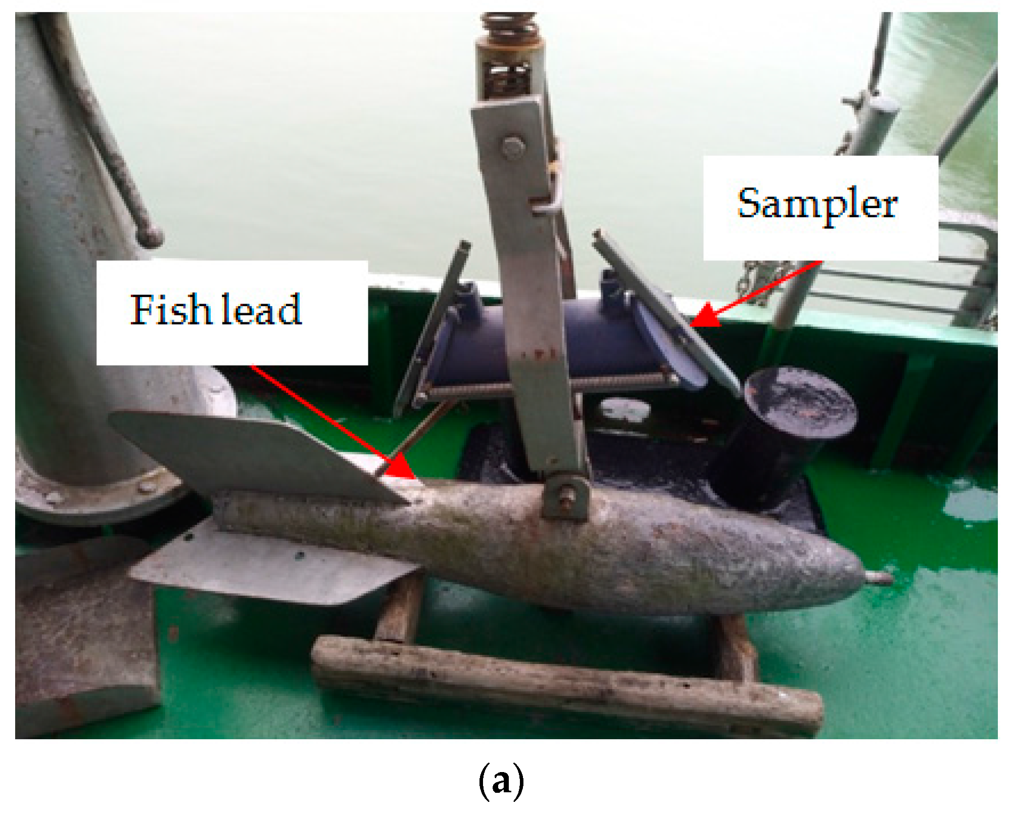
- Suspended sediments are sampled with samplers in the field, and its grain-size distributions are analyzed by the sieving method. All the sampling procedures should be finished within dozens of minutes, and sieving analyses should be finished following the manual operation. For all the five points measured before 2010 and the upper five points measured after 2010, the sampler shown in Figure 2a is adopted. For the two near-bed points measured after 2010, bottom-touched automatic-closing samplers shown in Figure 2b,c are adopted. With this kind of sampler (Figure 2b,c), the distances of the two near-bed points from the riverbed can be ensured. However, the potential disturbance on the riverbed when settling the sampler may still be questionable. Therefore, except a slowed down settling velocity of the sampler, the near-bed concentrations may be double-checked after sampling and grain-size analyses. The assumption is that the measured concentration is reliable only if the vertical concentration profiles of particles finer than 0.062 mm have no abrupt changing point in the near-bed region [17]. Thus, bed materials can be distinguished from suspended sediments, which may be caused by disturbance during the sampling processes.
2.3. Methodology
Methods of cumulative anomaly and SRCs are applied to investigate the changed sediment regime of un-saturated channel in reach scales. ADEs and the sediment-balance method are adopted to evaluate new challenges for the non-saturated channel.
2.3.1. Cumulative Anomaly
The cumulative anomaly has been widely applied to detect the trends and stages of time series [18]. For time series, the cumulative anomaly (Xt) for data point xi can be expressed as:
in which xi is the value of the time series; xm is the mean value of the series xi; and n is the length of the time series.
The mass curve of cumulative anomaly values describes the change process of a particular parameter by comparing it with the mean value of that parameter over the whole study period [18]. For instance, if the observed data of a given year is greater than the overall mean, the anomaly values will be positive and the mass curve will rise.
2.3.2. SRCs
The SRC is defined as the statistical relationship between SSC (kg·m−3) and discharge. SRCs are normally used to describe the flow-sediment relationships in river systems for various purposes [19]. The method is often applied to estimate the SSC or SSL in ungauged regions [20].
The power function of SRC is usually expressed as one of the following two formats:
in which Q is the discharge (m3·s−1), and e and f are the sediment rating coefficient and exponent, respectively. Linear regression, i.e., Equation (3), is often used to derive the values of the rating coefficient e and exponent f from empirical data (e.g., [21]). The e-parameter contains information on the conversion of Q into SSC, namely, the erosion severity index [22]. A high value of the e-parameter indicates easily-erodible materials and high loads of transported materials [20]. The exponent f-coefficient corresponds to the erosive power of the river and the influence on the sediment supplement. High values of the f-coefficient indicate a slight increase in discharge would significantly enhance the erosive power of the river [20]. Moreover, the f-coefficient is also related to climate, channel morphology, the grain-size distribution of sediments, and erodibility within the river basin [22].
2.3.3. ADEs
Three equations are adopted to evaluate the challenge in simulating the vertical concentration profiles in the unsaturated channel: the Rouse Equation, the Han Equation, and the fADE. These three equations may represent typical concentration profiles in equilibrium transport, non-equilibrium transport, and non-Fickion suspension in the non-equilibrium condition, respectively.
By assuming Fick’s first law for sediment diffusion in turbulence, the diffusion theory of sediment suspension can be expressed with traditional ADE model. The equation for equilibrium sediment transport can be expressed as:
in which S is the sediment concentration (W·L−3), y is the vertical coordinate (L), ω is the sediment settling velocity (L·T−1), and εsy is the sediment turbulent diffusion coefficient in the y direction (L·T−1).
By replacing εsy with the fluid eddy viscosity and assuming based on the Karman-Prandtl logarithmic velocity profile, Rouse et al. [4] obtained the analytical vertical concentration profile:
in which Sa is a reference concentration at a given height above the river bed (W·L−3), α is the reference height (L), H is the flow depth (L), κ is von Karman’s constant, and u∗ is the shear velocity (L·T−1). The frictional flow velocity can be calculated as , in which τb is the near-bed shear stress and is the water density. The Rouse equation, Equation (5), has been widely used for decades. However, its drawbacks are obvious: the concentration is calculated as zero at the water surface and infinity at the river bed. These drawbacks are caused by implicit assumptions, equilibrium sediment transport, and Fick’s first law. Extensive efforts have been put forward to improve the equation [10,23,24,25].
The assumption of equilibrium sediment transport limits its application in the field in which the sediment regime is far from equilibrium [26]. Among others, Han et al. [9] have modified Equation (4) to meet the non-equilibrium condition:
in which qs is the net flux due to the imbalance between downward sediment settling and upward turbulent dispersion. Han et al. [9] obtained the solution of Equation (6):
in which c is non-equilibrium coefficient defined as a function of the degree of saturation . is the depth-averaged sediment concentration (kg·m−3), and is the depth-averaged sediment capacity. If the saturation degree , c = 1; if , c > 1, which means the flow is unsaturated with sediment; and if , c < 1, which indicates an super-saturated flow. The von Karman’s constant κ is usually given a value of 0.408 for an unstratified flow.
According to Fick’s First Law, particles may make “local” jumps, as most particle jumps induced by turbulence are constrained to a small distance (Δy) in a given Δt according to the Central Limit Theorem (CLT), and Δy is characterized by the length of Representative Elementary Volume (REV) [27,28]. However, modern observations of coherent structures in turbulence have proven that high-speed currents may intermittently sweep the bed, carry much sediment, and eject directly into the upper part of the water column [27,29]. The non-Fickion suspension indicates that particles may make many “nonlocal” jumps in burst-like suspension events [27]. The non-Fickion suspension in non-equilibrium sediment suspension can be described by a fractional advection-dispersion equation (fADE) [27]:
in which α is the order of the fractional derivative (0 < α ≤ 1); (Lα·T−1) is the depth-averaged diffusivity expressed as follows:
We assume:
in which c0 is called the non-equilibrium coefficient, and c0 is a function of (S/S∗):
in which S∗ is the sediment transport capacity of flow; if S = S∗, then c0 = qs = 0, which means the flow reaches equilibrium; if S < S∗, then c0 > 0 and qs < 0, which means the flow is unsaturated with sediment; and if S > S∗, then c0 < 0 and qs > 0, which means flow is supper-saturated with sediment.
The analytical solution of Equation (8) is obtained:
in which Ea() is called Mittag-Leffler function (y ≤ a ≤ H), which can be calculated by series expansion or the MATLAB open-source code.
2.3.4. Contribution of Near-Bed Concentrations on SST Rate
The SST rate can be estimated with measured vertical concentration profiles, and the deposition/erosion amount of the channel can be estimated by the sediment balance method. Changed vertical concentration profiles in the unsaturated channel lead to new challenges in field surveying and estimating the SST rate. The field survey should be conducted according to its new characteristic (as extended measuring of near-bed zone by JHWRSB). The effect of the changed vertical concentration profiles on the SST rate can be estimated by evaluating the contribution of two near-bed concentrations on the SST rate:
in which Qs(7) and Qs(5) are cross-sectional SST rates by seven points and, artificially, by five points, respectively. The cross-sectional sediment flux can be estimated with all measured vertical profiles. The delta-shaped area between the left bank and the first vertical line from the left bank is also considered [17]. The delta-shaped area between the right bank and the last vertical line from the left bank is not considered due to the difficulty of identifying the right bank [17].
3. Change of the Sediment Regime
Vertical concentration profiles and SST rates are analyzed to evaluate the sediment regime of local and reach scales, respectively. Then, sediment rating curves are analyzed to investigate the availability of sediment for suspension from the riverbed.
3.1. Vertical Profiles of SSC
3.1.1. Remarkable Large Concentrations in the Near-Bed Zone
e depth-averaged concentration Savg (kg·m−3) is calculated as , in which Si is the measured concentration at each point in a vertical line (kg·m−3) and y is the vertical axis of the Cartesian coordinate system. The coordinate origin is located on the riverbed. To present the deviation of the near-bed concentration from the average, the relative concentration is defined as Sa/Savg, in which Sa is the measured concentration at the reference height. The reference height is the minimum distance of measuring points from the river bed. The reference height a equals 0.4–0.5 m for profiles measured before 2010, while the value is 0.1 m for profiles after 2010.
Figure 3 shows the typical vertical profiles measured at Shashi station before and after the impoundment of TGD. The relative concentrations (Sa/Savg) of these four vertical profiles are 2.47, 4.1, 2.10, and 1.52, respectively. Thus, remarkable large concentrations can be observed in the near-bed zone. The remarkable large near-bed concentration is defined by comparison to the vertical average concentration. This can be observed in vertical concentration profiles with large or small measured near-bed concentrations (3.01 kg·m−3 for Figure 3a and 0.041 kg·m−3 for Figure 3b).
The statistic characteristics of hundreds of vertical profiles are summarized in Table 2. Before TGD operation, the maximum relative concentrations (Sa/Savg) are 2.76 (Zhicheng), 2.30 (Shashi), and 3.62 (Jianli), respectively. After TGD operation, the maximum relative concentrations (Sa/Savg) are 15.05 (Shashi), and 14.45 (Jianli), respectively. The average relative concentrations before TGD are 1.35 (Shashi) and 1.57 (Jianli), respectively. These values jump to 3.22 (Shashi) and 4.89 (Jianli) after TGD, respectively. Thus, both the average and maximum values of relative concentrations (Sa/Savg) increase significantly after the impoundment of the TGD.
Relatively high concentrations near the bed region have also been pronounced in the estuary of YR, Qiantangjiang River, and the Taizhou sea area [30,31,32,33]. The near-bed concentration of the S-type vertical distribution is also relatively large [34]. However, the relative concentrations are relatively small (shown in Table 2). The maximum relative concentration (Sa/Savg) is approximately 4.3, and the minimum relative height of measured points from river bed is approximately 0.02. In total, the tailing phenomena in the unsaturated channel are much more apparent.
The coarsening of suspended sediment can be revealed by mean diameters of vertical profiles (shown in Table 2). For vertical lines measured at Jianli station, the average mean diameters after TGD range from 0.0087 mm to about 0.22 mm, while the values before TGD may range from 0.0037 mm to 0.07 mm. For vertical lines measured at Shashi station, the average mean diameters after TGD change from 0.0058–0.027 mm to 0.0098–0.224 mm. Thus, the coarsening process of suspended sediment after TGD operation is apparent, especially at Shashi station.
Both of the near-bed SSC and sediment flux are connected with hydrodynamic conditions [35]. Thus, hydrodynamic parameters (depth, velocity, and vertical average concentration) are also summarized in Table 2. The values of ω/u∗ vary dramatically (shown in Table 2). Remarkable large values of ω/u∗ indicate that relatively coarser particles may be suspended with a small bed shear velocity. Tang et al. [32] pointed out that the near-bed concentration may be more apparent when (ω/κu∗) > 5. Therefore, larger values of log(ω/u∗) in non-equilibrium channels contribute to remarkable large concentrations in the near-bed zone.
Normally, concentration at the water surface should be smaller than that at the riverbed. This means that the concentration gradient (estimated with d(Si − Si−1)/d(yi − yi−1)) should be negative. However, the occurrence of vertical concentration profiles with positive gradients increases (Table 3). For data measured before TGD, about 20% (Zhicheng, Shashi, and Jianli stations) vertical concentration profiles are characterized with positive gradients. For data measured after TGD, about 28–47% (Shashi and Jianli) of vertical concentration profiles are characterized with positive gradients (Table 3). The differential equation for vertical SSC distribution of non-uniform particles indicates that the concentration of finer particles group near the surface may be greater than that near the bed with wide grading non-uniformed suspended sediment [36]. Moreover, concentration gradients may be positive when the diameter of coarser particles is about eight times that of finer particles [36]. This indicates wide grading sediment particles in the non-equilibrium channel contribute to the remarkable large near-bed concentration.
3.1.2. Coarsening of Suspended and Bed Materials
Relatively large concentrations in the near-bed zone in estuary areas can be observed during tide periods and non-flood seasons [30]. Thus, the hydrologic condition (suspended sediment and bed materials) under which the remarkable large concentrations in the near-bed zone may occur is also analyzed.
With the operation of TGD, both the suspended and bed materials become much coarser, except for the dramatic decrease of the annual suspended sediment load (SSL) [37]. The temporal variation of suspended sediment size in the downstream channel may exhibit some complex processes [38]. This means that the saturation recovery process of fine sediments that responds to changing hydraulic conditions is different from that of the coarser one. Additionally, under non-uniform and non-equilibrium conditions, suspended sediment dynamics require a relatively large distance or time to approach equilibrium [13]. Thus, the variation trend of non-uniform sediment varies in different river reaches.
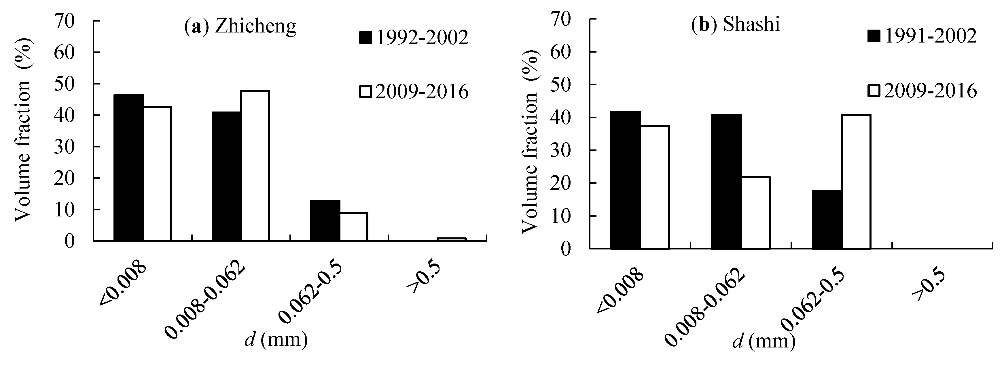
The mean diameter of SSC measured at Yichang station decreases from 0.009 mm (before impoundment) to 0.005 mm (2003–2008) [37]. Size distributions of suspended sediment and bed materials in the JJRR are shown in Figure 4 and Figure 5. For Zhicheng station, the proportion of grouped particles with diameters of 0.008–0.062 mm increases, while the proportions of finer (<0.008 mm) and coarser (0.062–0.5 mm) groups decreases. For Shashi station, the non-uniform sediment becomes a kind of wide grading (as shown in Figure 4b), as the proportion of grouped particles with diameters finer than 0.008 mm decreases and the proportion of grouped particles with diameters coarser than 0.062 mm increases. The mean diameter measured at Jianli station decreases from 0.009 mm (before impoundment) to 0.045 mm (2003–2008) [37]. This indicates that the coarser particles (>0.062 mm) around Shashi station have recovered by bed erosion. When flow transports the reach around Jianli station, the change of coarser particles (>0.062 mm) is much more apparent. Thus, wide grading suspended sediment at Shashi and Jianli stations may contribute to the remarkable large concentration in the near-bed zone.
The variations of volume fractions of bed materials indicate a remarkable coarsening process in the JJRR, especially the river reach of Zhicheng–Shashi (Figure 5). Zhang [30] pointed out that concentrations in the near-bed zone are more apparent with larger values of relative particle size (Di/Dm, particle-size over averaged particle size) of non-uniform sediment. Thus, the lifting and suspension of wide grading bed materials may also contribute to the remarkable large concentration in the near-bed region of the non-equilibrium channel.
3.2. Temporal Change of SSL
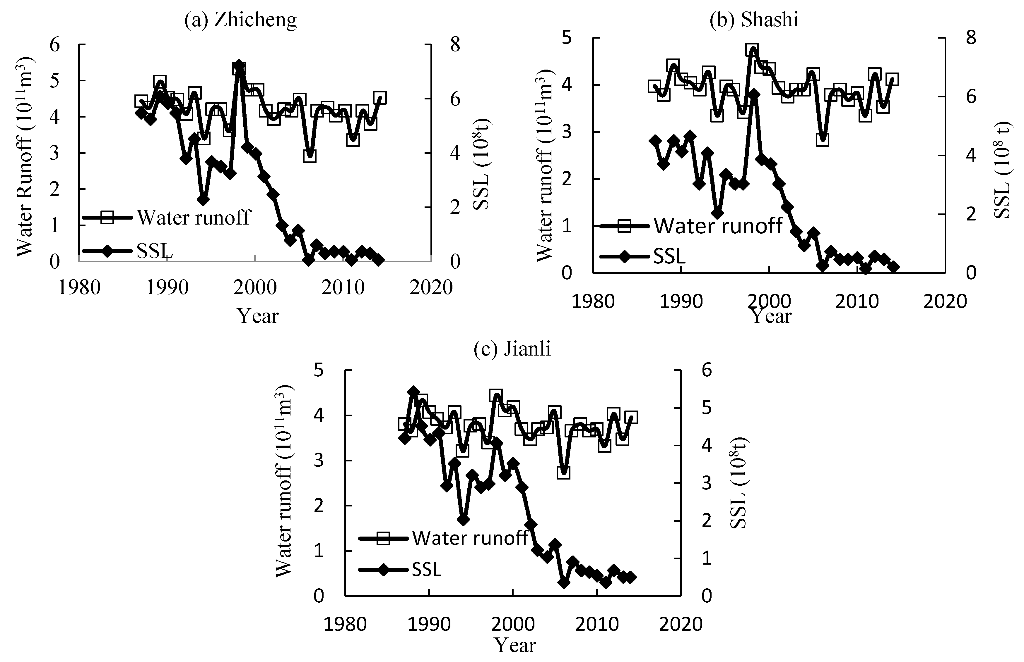
At the reach scale, the changed sediment regime can be described with temporal and spatial variations of SSL. The temporal and spatial variations of water runoff have also been analyzed to make a comparison. The temporal variation of water runoff and SSL show a decreasing trend, especially the SSL (Figure 6).
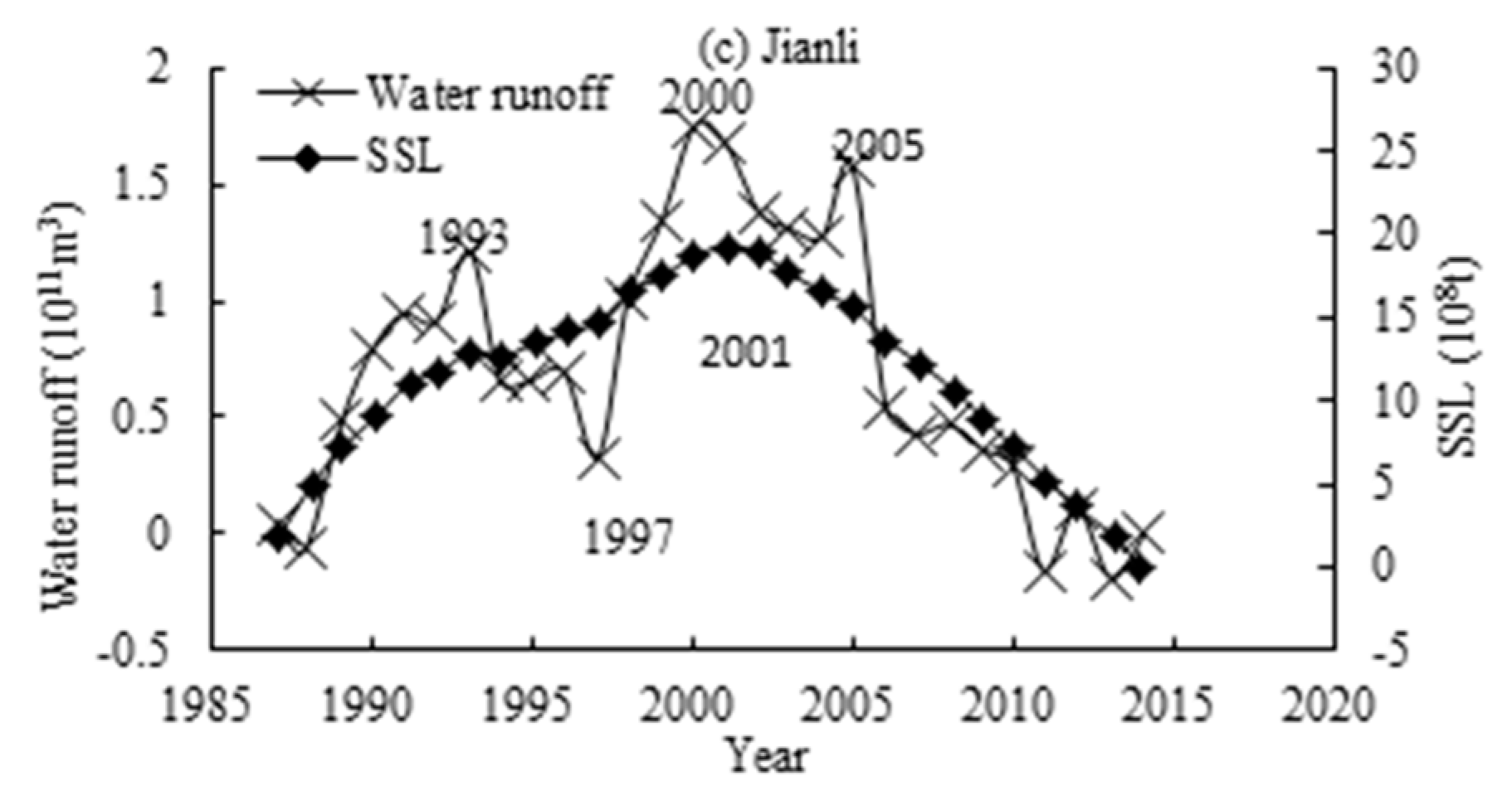
Figure 7 shows the mass curves of cumulative anomaly of annual runoff and SSL at the three stations (1987–2014). It shows that the water runoff and SSL show an increasing trend before 2000–2001 and then a decreasing trend after 2000–2001. Three Gorges Reservoir (TGR) was launched to construct in 1994, and TGD was completed and firstly impounded water in June 2003. The TGR started to operate regularly in June, 2006 and became fully operation in 2008. The other changing points of water runoff are 1993, 2005, and 2010, which are in accordance with the operation of TDR. The changing point of 1997 may be caused by the great 1998 flood, which was the highest in recorded history.
Thus, after 2005, both the runoff and SSL are less than the long-term average value.
3.3. Availability of Sediment Sources
The availability of weathered sediments in the unsaturated channel can be revealed by rating parameters. Thus, the SSC–Q rating curves with data measured before and after TGD operation at the JJRR is adopted to investigate the hydrological condition.
According to data measured in 2013, values of the f-parameter are 2.27 (Shashi) and 1.67 (Jianli), respectively, and values of the log(e)-parameter are −7.70 (Shashi) and −10.70 (Jianli), respectively (Figure 8). The long-term average values by Yang et al. [39] are illustrated as data before dam operation (Figure 8). The long-term average values of the log(e)-parameter and the f-parameter for Xinchang station are −1.92 and 1.17, respectively, and the values for Jianli station are −0.97 and 0.96, respectively [39]. Historical data adopted in the analysis of Yang et al. [39] were measured at four stations: Yichang (1950–1985), Xinchang (1956–1984), Jianli (1954–1986), and Chenglingji (1951–1982). According to Figure 6 and Figure 7, parameters by Yang et al. [39] may represent the hydrological conditions during the period before the changing point. Thus, with the operation of TGD, the values of the f-parameter increase while the values of the log(e)-parameter decrease.
Instantaneous SST rates are not only a function of the transport capacity of a river, but also of sediment availability [22]. For sediment rating parameters estimated through regression analysis, the e-coefficient is an erosion severity index in the river channel and is associated with the availability of weathered sediments in the basin area [22]. A high e-value indicates that this area is characterized with easily erodible materials and high loads of materials transported by runoffs [20]. The exponent f-coefficient corresponds to the erosive power of the river and the influence on the sediment supply from the entire basin surface. High values indicate a considerable increase in erosive power and sediment-carrying capacity with an increase in river discharge [20]. Thus, a slight increase in discharge enhances the erosive power of the river significantly. For the JJRR, the increased value of the f-parameter indicates a considerable increase of erosive power and sediment-carrying capacity with an increase in river discharge. A decreased value of the log(e)-parameter indicates a decreased availability of suspended sediments in the river channel.
The saturation recovery process in the JJRR can be described with Figure 4 and Figure 5, while the changed interactions between suspended sediment and bed material can be explained by the changed values of rating curves’ coefficients (Figure 8).
For river reaches around Zhicheng station, coarsening of bed material is obvious. As to its limited distance from the TGD dam (60 km), the saturation recovery process of suspended sediment is limited.
For river reaches around Shashi station, coarsening of bed material is also obvious. Finer-grouped suspended sediments (particles with diameter < 0.008 mm) are transported from the upper river reach instead of local bed materials. Coarser suspended particles (with diameter of 0.062–0.05 mm) have recovered, which are eroded from local bed materials as an increased value of the sediment rating exponent (f-parameter).
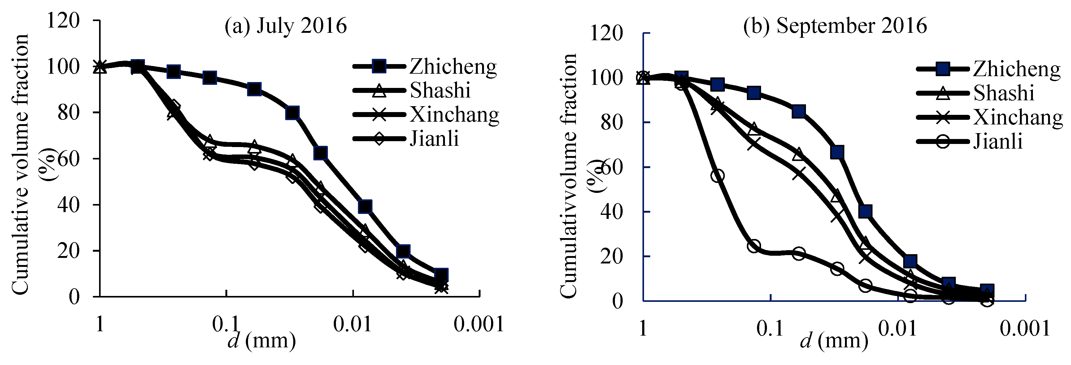
For river reaches around Jianli station, the coarsening of the bed material is limited. The coarsening of suspended sediment is obvious, especially after flooding (Figure 9). Coarser suspended particles (with diameter of 0.062–0.05 mm) may come from the erosion of the local river bed and transportation from upper reaches by an increased value of the f-parameter.
The variability in the relationship between the sediment concentration and water discharge (namely hysteretic patterns) has also been used to explain the variability of sediment sources from one flood to another [40]. Whitaker et al. [41] compared the estimated sediment yield for an un-sampled flood event, a single-event surrogate SSC–Q rating curve, or a long-term SSC–Q rating curve. Analysis revealed that the long-term SSC–Q rating curve estimates approximately 37% higher than the single-event SSC–Q estimates, which indicates a high degree of uncertainty. Analysis shows a high variability in the rating curve between similar floods [41]. This is the reason for erosion during the flood season.
4. Future Challenges
4.1. Accurate Measuring in Field Surveys
Accurate measurement of vertical concentration profiles is important for investigating the vertical distribution of SSC and the accurate estimation of sediment transport. For the field survey in the JJRR, the two near-bed points are measured with constant distances of 0.5 m and 0.1 m from the bed, respectively. However, the small distances may be doubtful due to difficulties in distinguishing the bed material and suspended sediment, especially when the bed is disturbed during settling sampling. Equipment and criteria adopted in the field survey have been described in detail in the Methodology section, and their availability and methods of improvement with regard to accuracy in the future are discussed.
The availabilities of ADCP and GNSS have been certified by field surveys conducted by other researchers. The error of hydrologic measurement with ADCP is ±1%, and the random uncertainty is 2–5% for measuring cross-sections in the middle and lower YR channel [42]. The integrated system (GPS and ADCP) delivers positioning with <15 cm accuracy vertically and <30 cm horizontally [42]. For GNSS, the differences between coordinates of the ground control points estimated using RTK–GNSS, and those computed from the classical topographic measurements during processing of the photogrammetric blocks have been analyzed by Pagliari et al. [43]. It was pointed out that an RTK–GNSS survey may be sufficient to reach the requested tolerance [43]. GNSS receivers have been adopted in field surveys in recent years, as their main advantages are of being faster, cheaper, and easier to use during the surveying phase than classical topographic survey [43,44]. For sediment grain-size analysis, the results by LPSA and sieving methods are comparable when particles are spherical [45]. Sieving methods for coarser particles are more acceptable than for finer ones [45]. Thus, the sieving method adopted by JHWRSB for fine suspended particles needs further verification.
In total, various efforts have being applied to measure the SSC profiles in field surveying, including methods and instrumentation [46,47,48]. Some new field instrumentation, including magnetic tracers, drone-based or plane-based topography surveys, and video analysis by spectral cameras can also be used to measure sediment transport and morphology evolution in future field surveys [49]. Except for these new instruments, already existing instruments can also be used with more details. For instance, ADCPs are increasingly used to measure the three-dimensional velocity distribution and sediment transport by measuring the Doppler shift in the backscattered signals from an array of acoustic beams [49,50]. According to the backscatter intensity of ADCP beams, SSC can also be estimated with inversion [51].
4.2. Describing Vertical Concentration Profiles
The vertical distribution of SSC needs to be described accurately for an accurate simulation of channel migration, i.e., a one-dimensional simulation for the transport of sediment mixture in non-equilibrium conditions [52]. Thus, finding a proper way to describe the vertical concentration profiles of the unsaturated channel is one of the key problems for hydraulic researchers [53].
Measured sediment profiles are compared with calculations by three equations, i.e., the Rouse Equation (Equation (5)), the Han Equation (Equation (7)), and the new fADE (Equation (12)). Figure 10 indicates the Rouse Equation is not applicable in the non-equilibrium reach. Compared to the Rouse Equation, the Han Equation for non-equilibrium, sediment-laden flow performs better in the upper part of a vertical but underestimates the concentration near the river bed, i.e., within 10% of the water depth. The fADE is able to characterize the dynamics of the non-equilibrium sediment suspension in “starving” river reaches.
No doubt, Equation (7) for non-equilibrium conditions can offer a better description of sediment profiles in river reaches with unsaturated or oversaturated flows. The inaccurate prediction is partly due to our poor understanding of the mechanism of sediment suspension, i.e., the spatially-stochastic transport behavior in sediment dispersion. For the changed sediment regime of the JJRR, more efforts are required to improve the description of vertical profiles of SSC, especially the physical processes. Additionally, “nonlocal” jumps in burst-like suspension events indicate that bursting eddies may sweep particles from the water bottom and directly eject them to the upper part of water bodies, which may lead to ecological-related problems. The ecology consequences include water quality of the riverine ecosystems, as nutrients and pollutants are often closely connected with sediments [49]. The three outlets (Songzikou, Taipingkou, and Ouchikou) have a special setting of the surface water system between YR and Dongting Lake, and the three diversion channels could interact directly with the lake. Thus, it may also have a profound impact on the biological connection between the main stream and the downstream lakes of Poyang and Dongting.
4.3. Estimating SST Rate
Measuring and describing the vertical SSC profiles accurately is also imperative to the quantification of the SST rate [2]. If near-bed concentrations are not measured or simulated correctly, the estimation of the SST rate may also be influenced.
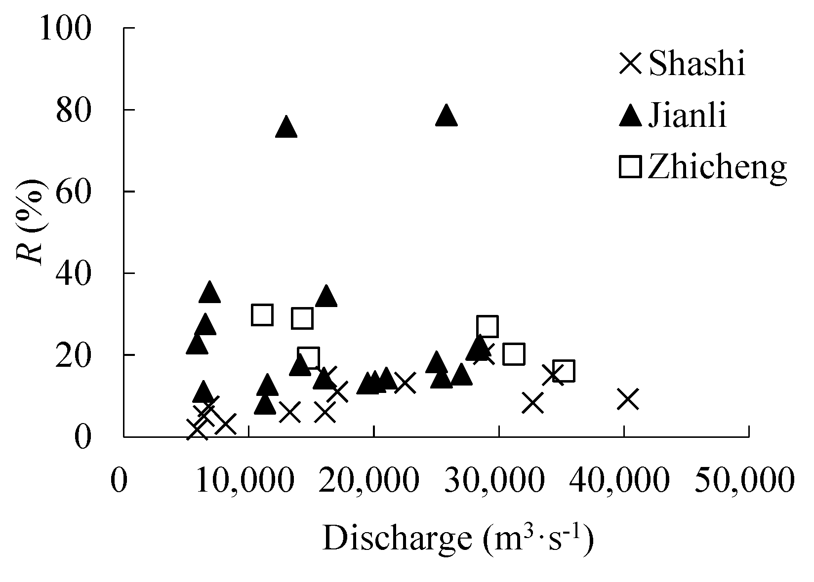
Figure 11 shows the estimated contributions by two near-bed points. Both of these two extremely large ratios (larger than 60%) occurred at Jianli station in 1996. For these two sections, the estimated sectional average velocities are different from measured data with a large deviation. This indicates that the assumption for Equation (13) is not adoptable in these two cross-sections. Thus, these two sections are excluded from discussion. Figure 11 shows that, if the near-bed concentrations are not included, the sediment flux may be underestimated by approximately 23.5% (Zhicheng), 9.35% (Shashi), and 18.68% (Jianli), respectively. Thus, for the unsaturated JJRR, sediment concentration within 10% of the water depth from the riverbed cannot be ignored. Otherwise, it will lead to underestimated results when calculating the erosion/deposition of the JJRR by the sediment-transport balance method and volume method. Additionally, an underestimated SST rate at Zhicheng station may also lead to overestimated sedimentation in the TGR, which is important for the water storage capacity of the reservoir. The reservoir’s functions of water supply, energy production, navigation, flood control, and increased maintenance costs are correlated with the reservoir’s water storage capacity [49]. Thus, underestimated sedimentation at Zhicheng station may also affect the reservoir’s waterway systems, hydraulic schemes, intakes and outlets, and flow regulation [49].
Fortunately, the influence of near-bed concentration on estimating sediment flux can also be verified by comparing the estimated deposition with the sediment-balance method and the geometric method.
Based on the hydrology data and geometry data measured in 2002–2008, contributing factors that may cause deviation during estimating deposition were distinguished [54,55]. Yuan et al. [53] pronounced that the contribution ratio by near-bed concretion varies in different hydrology years and river reaches (Table 4). For a certain hydrological station, the contribution ratios may also vary with the inflow condition. In total, they partially verified the reliability of measured vertical concentration profiles by comparing contribution ratios.
When suspension index A = ω/(βku∗) = 2.0, suspended sediment may concentrate in areas with a distance of 0.2 times of the water depth from the riverbed, in which β is a coefficient for non-uniform sediment [30]. The near-bed concentration may affect the estimated sediment load only if A > 0.15 [30]. If A = 2.0, the ratio of near-bed transportation over the total transportation is approximately 30% [30]. The values of ω/u∗ with data measured after TGD in Table 2 are much larger than the criteria by Zhang [30], and a large contribution of the near-bed transportation over the total transportation in Figure 11 can be certified. The ratio of the near-bed transportation over the total transportation is approximately 25% when Di/Dm > 3, in which Di/Dm is the particle size the over average size [30]. The wide grading distribution of SSC after TGD (as shown in Figure 4 and Figure 5) also indicates a large contribution to the total transportation. Thus, the potential doubt that refers to difficulties in distinguishing bed material and suspended sediment can partially be certified. Moreover, the impact of a remarkable large near-bed concentration must be given more attention in the future, especially at river reaches around Shashi station.
In total, fluvial and dynamic characteristics of distinct, large concentrations in near-bed regions may affect sediment flux, erosion/deposition estimation, sediment rating curve, and the channel geometry followed. This brings river engineers a lot of new problems, i.e., degradation of navigation, and dramatic bank erosion [56]. Additionally, the estimation of erosion in the JJRR has a profound impact on the hydrologic connection between the middle YR and Dongting Lake [57].
5. Conclusions
Sediment regime of the JJRR has changed dramatically with the operation of TGD. Based on daily and vertical concentration data at the three hydrological stations (Zhicheng, Shashi, and Jianli) in the JJRR, the sediment regime and its potential challenges are analyzed in this study. The conclusions can be summarized as follows:
- (1)
- In the unsaturated JJRR, measurements have revealed anomalous vertical profiles of SSC, as the near-bed concentrations normalized with the vertical average concentration are dramatically larger than that of the pre-equilibrium channel. The near-bed concentration (within 10% of the water depth from the river bed) may reach up to 15 times that of the vertical average concentration in the non-equilibrium channel.
- (2)
- In the unsaturated JJRR, the combination of wide grading suspended sediment and coarsened bed materials in non-equilibrium channel contribute to a remarkably large concentration in the near-bed zone. For the river reach around Shashi station, the remarkably large near-bed concentration is more apparent.
- (3)
- More detailed measurements or new measuring technologies may assist in the accurate measurement of vertical concentration profiles. A fractional dispersion equation may help to provide accurate descriptions. The outcomes can provide useful information for modeling the morphologic change of the JJRR.
Acknowledgments
The financial support from National Key R&D Program of China (no. 2016YFC0402303); and the National Natural Science Foundation of China (Nos. 51579230, 51779242, 51509234, 41330751 and 51479179).
Author Contributions
L.H. and D.C. conceived and designed the paper, S.Z. analyzed the data, M.L. contributed to figures, G.D. provided materials of vertical concentration, and L.H. wrote the paper.
Conflicts of Interest
The authors declare no conflict of interest.
References
- Schumm, S.A. The Fluvial System; Wiley: New York, NY, USA, 1977. [Google Scholar]
- McLean, S.R. Depth-integrated suspended load calculations. J. Hydraul. Eng. 1991, 117, 1440–1458. [Google Scholar] [CrossRef]
- Papanicolaou, A.N.; Elhakeem, M.; Krallis, G.; Prakash, S.; Edinger, J. Sediment transport modelling review-current and future developments. J. Hydraul. Eng. ASCE 2008, 134, 1–14. [Google Scholar] [CrossRef]
- Rouse, H. Modern conceptions of the mechanics of fluid turbulence. Trans. Am. Soc. Civ. Eng. 1938, 102, 463–543. [Google Scholar]
- Hunt, J.N. On the turbulent transport of sediment in open channel. Proc. R. Soc. Lond. A 1954, 224, 1158. [Google Scholar] [CrossRef]
- Aragon, J.A.G.; Salazar, S.S.; Reyes, P.M.; Delgado, C.D. Concentration profiles of suspended sediments calculation in non-uniform sediments, nonequilibrium situations. Ing. Hidraul. Mex. 2000, 15, 29–35. [Google Scholar]
- Maleki, F.S.; Khan, A.A. 1-D coupled non-equilibrium sediment transport modelling for unsteady flows in the discontinuous Galerkin framework. J. Hydrodyn. 2016, 28, 534–543. [Google Scholar] [CrossRef]
- Nicholad, A.P.; Clarke, L.; Quine, T.A. A numerical modelling and experimental study of flow width dynamics on alluvial fans. Earth Surf. Process. Landf. 2009, 34, 1985–1993. [Google Scholar] [CrossRef] [Green Version]
- Han, Q.W.; Chen, X.J.; Xue, X.C. On the vertical distribution of sediment concentration in non-equilibrium transportation. Adv. Water Sci. 2010, 21, 512–523. [Google Scholar]
- Zhao, L.J.; Wu, G.Y.; Wang, J.Y. Review and prospect of vertical distribution by non-equilibrium sediment concentration theory. J. Hydroelectr. Eng. 2015, 34, 63–69. [Google Scholar]
- Regüés, D.; Nadal-Romero, E. Uncertainty in the evaluation of sediment yield form badland areas: Suspended sediment transport estimated in the Araguás catchment (central Spanish Pyrenees). Catena 2013, 106, 93–100. [Google Scholar] [CrossRef]
- Zhu, H.W.; Cheng, P.D.; Li, W.; Chen, J.H.; Pang, Y.; Zhang, D.W. Empirical model for estimating vertical concentration profiles of re-suspended, sediment-associated contaminants. Acta Mech. Sin. 2017, 33, 846–854. [Google Scholar] [CrossRef]
- Cheng, C.; Huang, H.M.; Liu, C.Y.; Jiang, W.M. Challenges to the representation of suspended sediment transfer using a depth-averaged flux. Earth Surf. Process. Landf. 2016, 41, 1337–1357. [Google Scholar] [CrossRef]
- Wu, W. Depth-averaged two-dimensional numerical modelling of unsteady flow and nonuniform sediment transport in open channels. J. Hydraul. Eng. 2004, 130, 1013–1024. [Google Scholar] [CrossRef]
- Tayfur, G.; Singh, V.P. Transport capacity models for unsteady and non-equilibrium sediment transport in alluvial channels. Comput. Electron. Agric. 2012, 86, 26–33. [Google Scholar] [CrossRef]
- Singh, A.K.; Kothyari, U.C.; Raju, K.G.R. Rapidly varying transient flows in alluvial rivers. J. Hydraul. Res. 2004, 42, 473–486. [Google Scholar] [CrossRef]
- He, L. Quantifying the effects of near-bed concentration on the sediment flux after the operation of the Three Gorges Dam, Yangtze River. Water 2017, 9, 986. [Google Scholar] [CrossRef]
- He, Y.; Wang, F.; Tian, P.; Mu, X.M.; Gao, P.; Zhao, G.J.; Wu, Y.P. Impact assessment of human activities on runoff and sediment of Beiluo River in the Yellow River Based on Paired Years of Similar Climate. Pol. J. Environ. Stud. 2016, 25, 121–135. [Google Scholar] [CrossRef]
- Wang, H.J.; Yang, Z.S.; Wang, Y.; Saito, Y.; Liu, J.P. Reconstruction of sediment flux from the Changjiang (Yangtze River) to the sea since the 1860s. J. Hydrol. 2008, 349, 318–332. [Google Scholar] [CrossRef]
- Iadanza, C.; Napolitano, F. Sediment transport time series in the Tiber River. Phys. Chem. Earth 2006, 31, 1212–1227. [Google Scholar] [CrossRef]
- Desilets, S.L.E.; Nijssen, B.; Ekwurzel, B.; Ferre, T.P.A. Post-wildfire changes in suspended sediment rating curves: Sabino Canyon, Arizona. Hydrol. Process. 2007, 21, 1413–1423. [Google Scholar] [CrossRef]
- Asselman, N.E.M. Fitting and interpretation of sediment rating curves. J. Hydrol. 2000, 234, 228–248. [Google Scholar] [CrossRef]
- Huang, S.H.; Sun, Z.L.; Xu, D.; Xia, S.S. Vertical distribution of sediment concentration. J. Zhejiang Univ. Sci. A 2008, 9, 1560–1566. [Google Scholar] [CrossRef]
- Wilson, K.C. Rapid increase in suspended load at high bed shear. J. Hydraul. Eng. 2005, 131, 46–51. [Google Scholar] [CrossRef]
- Brown, G.L. Approximate profile for nonequilibrium suspended sediment. J. Hydraul. Eng. 2008, 134, 1010–1014. [Google Scholar] [CrossRef]
- Jobson, H.E.; Serge, W.W. Predicting concentration profiles in open channels. J. Hydraul. Div. 1970, 96, 1983–1996. [Google Scholar]
- Chen, D.; Sun, H.; Zhang, Y. Fractional dispersion equation for sediment suspension. J. Hydrol. 2013, 491, 13–22. [Google Scholar] [CrossRef]
- Nie, S.Q.; Sun, H.G.; Zhang, Y.; Chen, D.; Chen, W.; Chen, L.; Schaefer, S. Vertical distribution of suspended sediment under steady flow: Existing theories and fractional derivative model. Discret. Dyn. Nat. Soc. 2017. [CrossRef]
- Noguchi, K.; Nezu, I. Particle-turbulence interaction and local particle concentration in sediment-laden open-channel flows. J. Hydro-Environ. Res. 2009, 3, 54–68. [Google Scholar] [CrossRef]
- Sun, Z.L.; Zhang, C.F.; Du, L.H.; Xu, D. Transport rate of nonuniform suspended load. Shuili Xuebao 2016, 47, 501–508. [Google Scholar]
- Dong, X.T.; Li, R.J.; Fu, G.C.; Zhang, H.C. Relationship between vertical distribution of velocity and sediment concentration of sediment-laden flow. J. Hohai Univ. Natl. Sci. 2015, 43, 371–376. [Google Scholar] [CrossRef]
- Tang, M.L.; Cao, H.Q.; Li, Q.Y.; Zhai, W.L. Vertical distribution of suspended sediment in middle reaches of Yangtze River. Yangtze River 2017, 48, 6–11. [Google Scholar]
- Xia, Y.F.; Xu, H.; Chen, Z.; Wu, D.W.; Zhang, S.Z. Experimental study on suspended sediment concentration and its vertical distribution under spilling breaking wave actions in silty coast. China Ocean Eng. 2011, 25, 565–575. [Google Scholar] [CrossRef]
- Feng, Q.; Xiao, Q.L. An new S-type vertical distribution of suspended sediment concentration. J. Sedim. Res. 2015, 1, 19–24. [Google Scholar]
- Parsons, A.J.; Cooper, J.; Wainwright, J. What is suspended sediment? Earth Surf. Process. Landf. 2015, 40, 1417–1420. [Google Scholar] [CrossRef] [Green Version]
- Zhang, X.F.; Tan, G.M. Characteristics of vertical concentration distribution of non-uniform particles. Shuli Xuebao 1992, 10, 48–52. [Google Scholar]
- Han, J.Q.; Sun, Z.H.; Li, Y.T.; Tang, J.W. Changed and caused of lower water level in Yichang–Chenglingji reach after impounding of Three Gorges Reservoir. Eng. J. Wuhan Univ. 2011, 44, 685–695. [Google Scholar]
- Xu, J.X. Complex behaviour of suspended sediment grain size downstream from a reservoir: An example from the Hanjiang River, China. Hydrol. Sci. J. 1996, 41, 837–849. [Google Scholar]
- Yang, G.F.; Chen, Z.Y.; Yu, F.; Wang, Z.; Zhao, Y.; Wang, Z. Sediment rating parameters and their implications: Yangtze River, China. Geomorphology 2007, 85, 166–175. [Google Scholar] [CrossRef]
- Seeger, M.; Errea, M.-P.; Begueria, S.; Arnaez, J.; Marti, C.; Garcia-Ruiz, J.M. Catchment soil moisture and rainfall characteristics as determinant factors for discharge/suspended sediment hysteretic loops in a small headwater catchment in the Spanish Pyrenees. J. Hydrol. 2004, 288, 299–311. [Google Scholar] [CrossRef] [Green Version]
- Whitaker, A.C.; Sato, H.; Sugiyama, H. Changing suspended sediment dynamics due to extreme flood events in a small pluvial-nival system in northern Japan. Sedim. Dyn. Chang. Environ. 2008, 325, 192–199. [Google Scholar]
- Zhang, Q.; Shi, Y.F.; Xiong, M. Geometric properties of river cross sections and associated hydrodynamic implications in Wuhan-Jiujiang river reach, the Yangtze River. J. Geogr. Sci. 2009, 19, 58–66. [Google Scholar] [CrossRef]
- Pagliari, D.; Rossi, L.; Passoni, D.; Pinto, L.; De Michele, C.; Avanzi, F. Measuring the volume of flushed sediments in a reservoir using multi-temporal images acquired with UAS, Geomatics. Nat. Hazards Risk 2017, 8, 150–166. [Google Scholar] [CrossRef]
- Bandini, F.; Jakobsen, J.; Olesen, D.; Reyna-Gutierrez, J.A.; Bauer-Gottwein, P. Measuring water level in rivers and lakes from lightweight unmanned aerial vehicles. J. Hydrol. 2017, 548, 237–250. [Google Scholar] [CrossRef]
- Li, W.K.; Wu, Y.X.; Huang, Z.M.; Fan, R.; Lv, J.F. Measurement results comparison between Laser Particle Analyzer and Sieving method in particle size distribution. Zhongguo Fenti Jishu 2007, 13, 10–13. [Google Scholar]
- Pedocchi, F.; Garcia, M.H. Acoustic measurement of suspended sediment concentration profiles in an oscillatory boundary layer. Cont. Shelf Res. 2012, 46, 87–95. [Google Scholar] [CrossRef]
- Yu, Q.; Flemming, B.W.; Gao, S. Tide-induced vertical suspended sediment concentration profiles: Phase lag and amplitude attenuation. Ocean Dyn. 2011, 61, 403–410. [Google Scholar] [CrossRef]
- Pitarch, J.; Odermatt, D.; Kawak, M.; Wuest, A. Retrieval of vertical particle concentration profiles by optical remote sensing: A model study. Opt. Express 2014, 22, 947–959. [Google Scholar] [CrossRef] [PubMed]
- Schleiss, A.; Franca, M.J.; Juez, C.; Cesare, G. Reservoir sedimentation. J. Hydraul. Res. 2016, 54, 595–614. [Google Scholar] [CrossRef]
- Togneri, M.; Lewis, M.; Neill, S.; Masters, I. Comparison of ADCP observations and 3D model simulations of turbulence at a tidal energy site. Renew. Energy 2017, 114, 273–282. [Google Scholar] [CrossRef]
- Jin, W.F.; Liang, C.J.; Zhou, B.F.; Li, J.D. Measurement and analysis of high suspended sediment concentration in Jintang channel with vessel-mounted ADCP. J. Mar. Sci. 2009, 27, 31–39. [Google Scholar]
- Merkhali, S.P.; Ehteshami, M.; Sadrnejad, S.A. Assessment quality of a nonuniform suspended sediment transport model under unsteady flow condition (case study: Aras River). Water Environ. J. Promot. Sustain. Solut. 2015, 29, 189–498. [Google Scholar] [CrossRef]
- Eggenhuisen, J.T.; McCaffrey, W.D. The vertical turbulence structure of experimental turbidity currents encountering basal obstructions: Implications for vertical suspended sediment distribution in non-equilibrium currents. Sedimentology 2012, 59, 1101–1120. [Google Scholar] [CrossRef]
- Yuan, Y.; Zhang, X.F.; Duan, G.L. Modifying the channel erosion and deposition amount of Yichang–Jianli reach calculated by sediment discharge method. J. Hydroelectr. Eng. 2014, 33, 163–169. [Google Scholar]
- Duan, G.L.; Peng, Y.B.; Guo, M.J. Comparative analysis on riverbed erosion and deposition amount calculated by different methods. J. Yangtze River Sci. Res. Inst. 2014, 31, 108–118. [Google Scholar]
- Xia, J.Q.; Deng, S.S.; Lu, J.Y.; Xu, Q.X.; Zong, Q.L.; Tan, G.M. Dynamic channel adjustments in the Jingjiang reach of the middle Yangtze River. Sci. Rep. 2016, 6, 22802. [Google Scholar] [CrossRef] [PubMed]
- Li, Y.Y.; Yang, G.S.; Li, B.; Wan, R.R.; Duan, W.L.; He, Z. Quantifying the effects of channel change on the discharge diversion of Jingjiang Three outlets after the operation of the Three Gorges Dam. Hydrol. Res. 2016, 47, 161–174. [Google Scholar] [CrossRef]
Figure 1.
Sketch of the YR (a) and JJRR (b); (b) is drawn from [17].
Figure 1.
Sketch of the YR (a) and JJRR (b); (b) is drawn from [17].
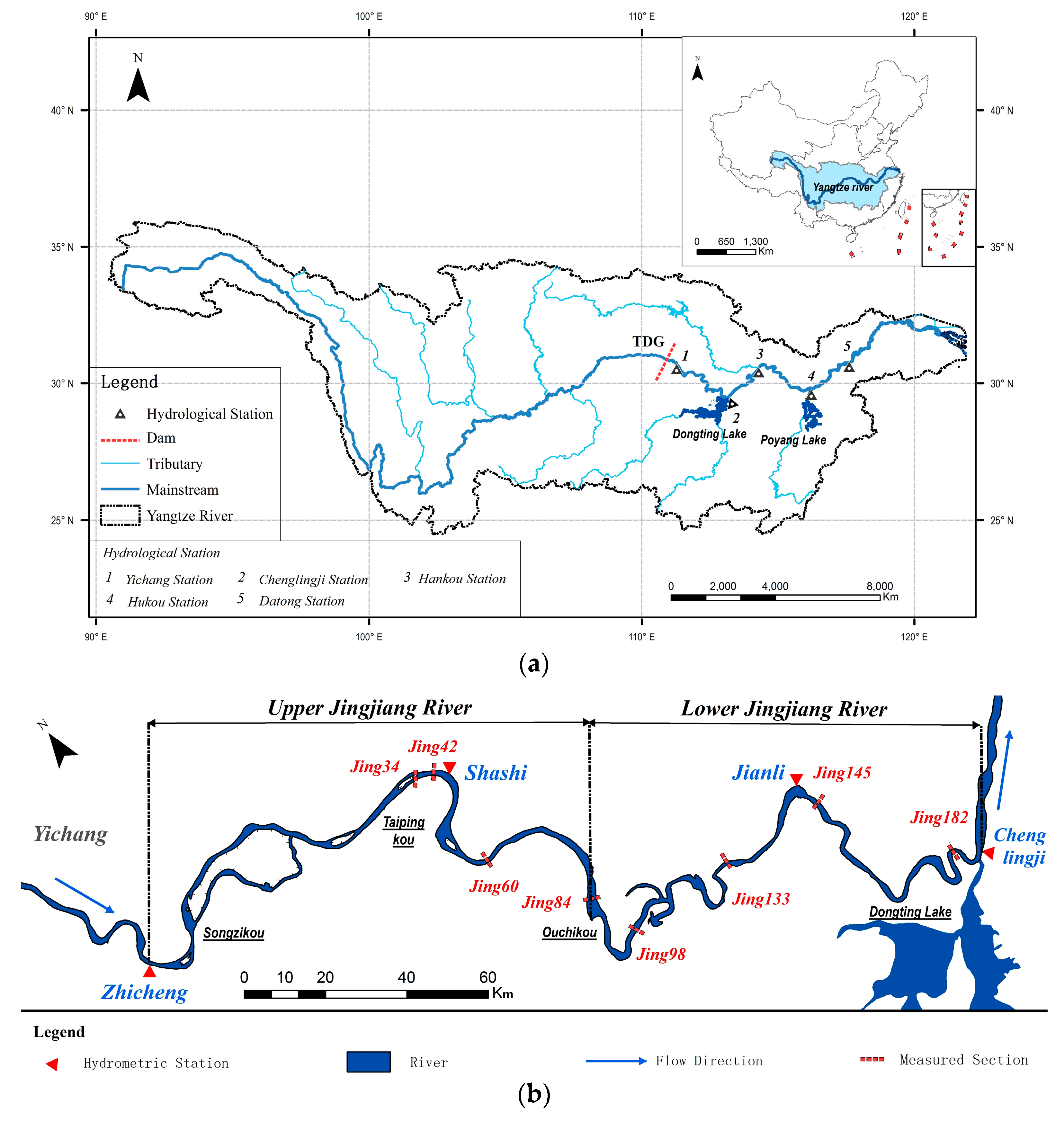
Figure 2.
Samplers for suspended sediment in the field survey; (a) is the sampler with fish lead, and (b,c) are the samplers for sampling suspended sediment at the two near-bed points (different camera angles).
Figure 2.
Samplers for suspended sediment in the field survey; (a) is the sampler with fish lead, and (b,c) are the samplers for sampling suspended sediment at the two near-bed points (different camera angles).

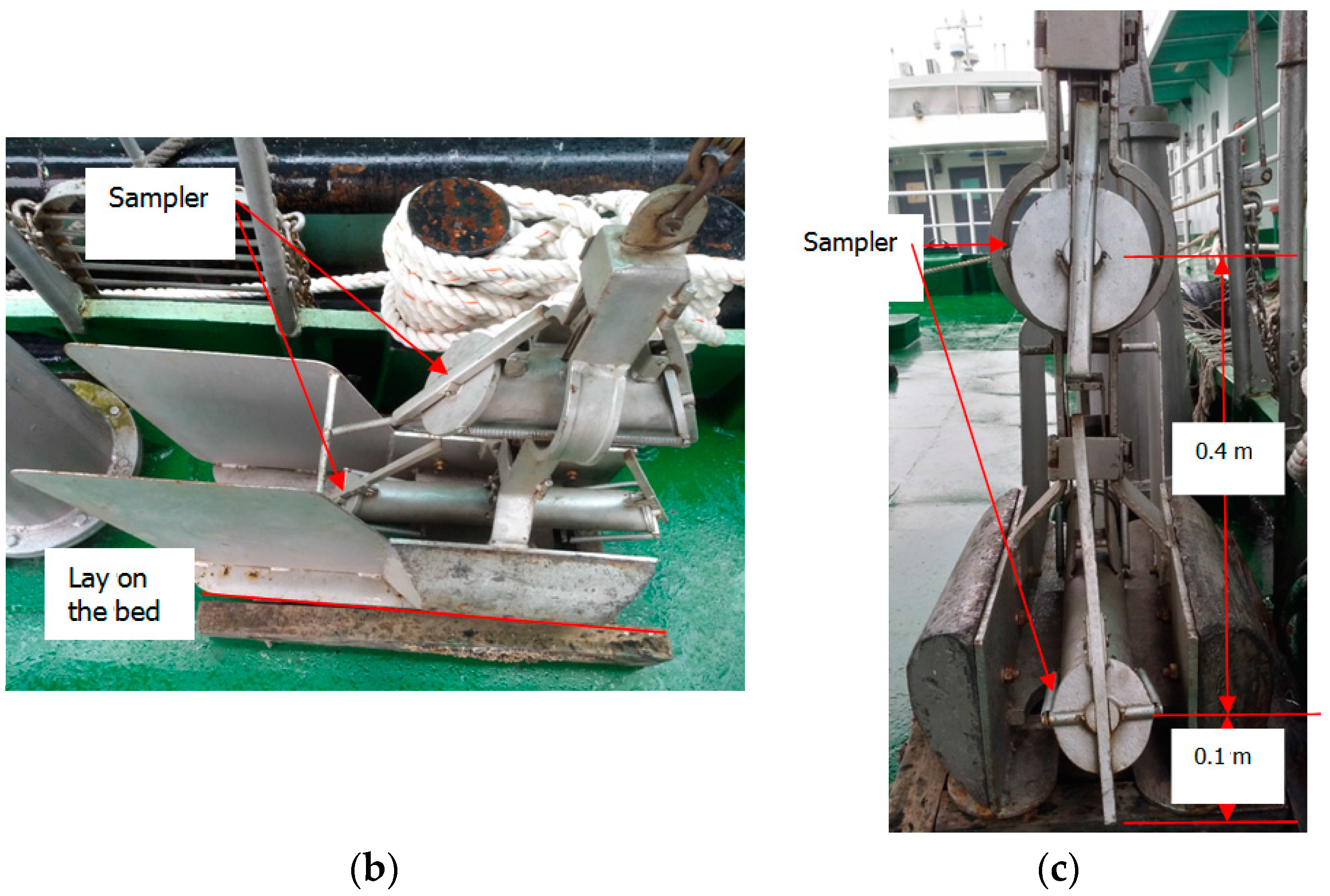
Figure 3.
Typical measured vertical profiles of SSC and vertical averaged concentration in the JJRR, measured at Shashi hydrological station before (c,d) and after 2010 (a,b).
Figure 3.
Typical measured vertical profiles of SSC and vertical averaged concentration in the JJRR, measured at Shashi hydrological station before (c,d) and after 2010 (a,b).
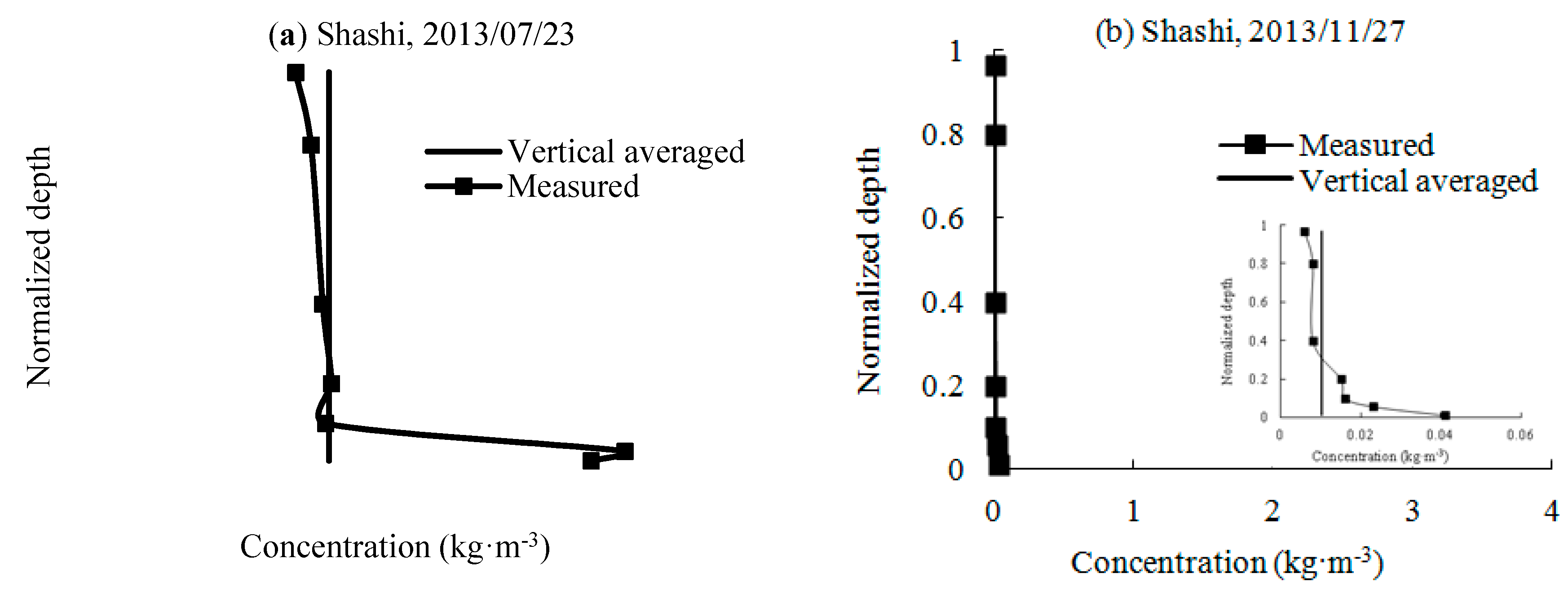
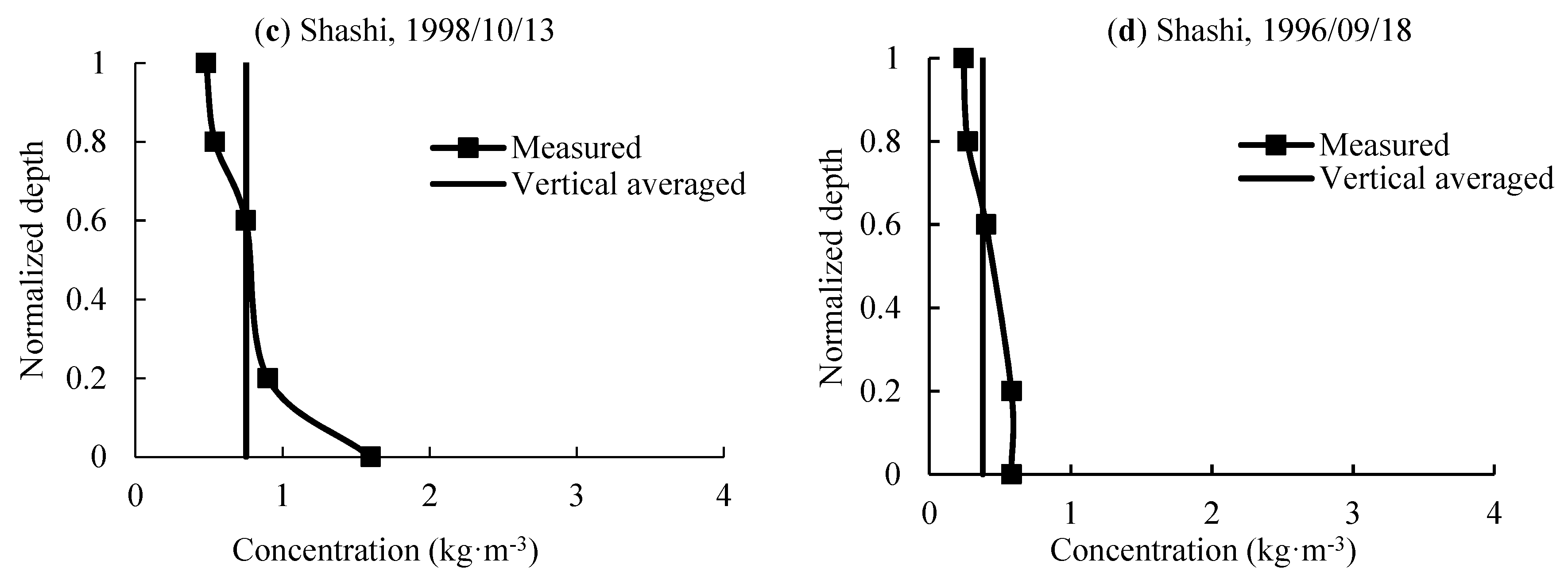
Figure 4.
Volume fractions of suspended sediment measured at Zhicheng (a), Shashi (b), and Jianli (c) stations.
Figure 4.
Volume fractions of suspended sediment measured at Zhicheng (a), Shashi (b), and Jianli (c) stations.

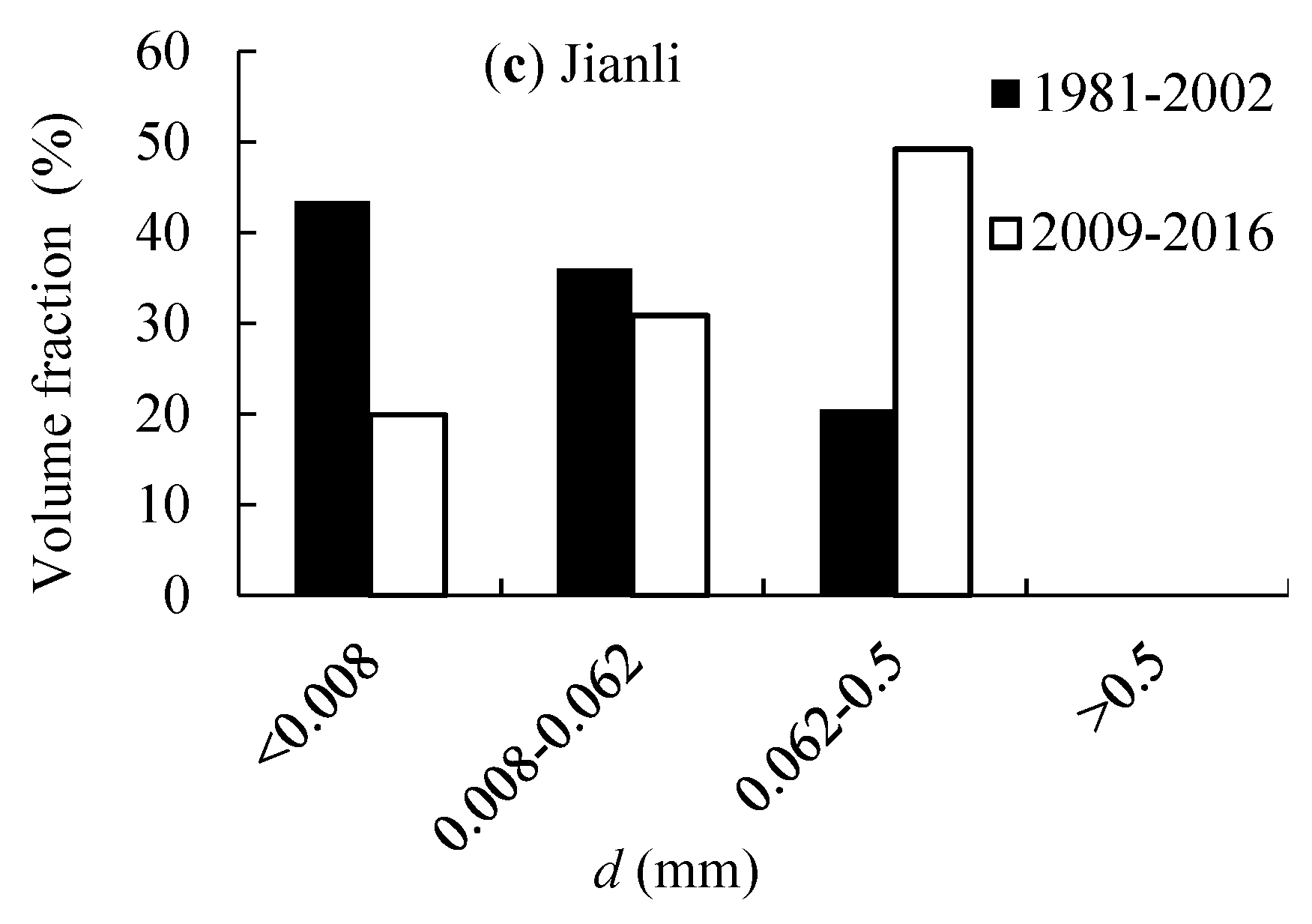
Figure 5.
Cumulative volume fractions of bed materials measured at Zhichegn (a), Shashi (b), and Xinchang (c) stations.
Figure 5.
Cumulative volume fractions of bed materials measured at Zhichegn (a), Shashi (b), and Xinchang (c) stations.
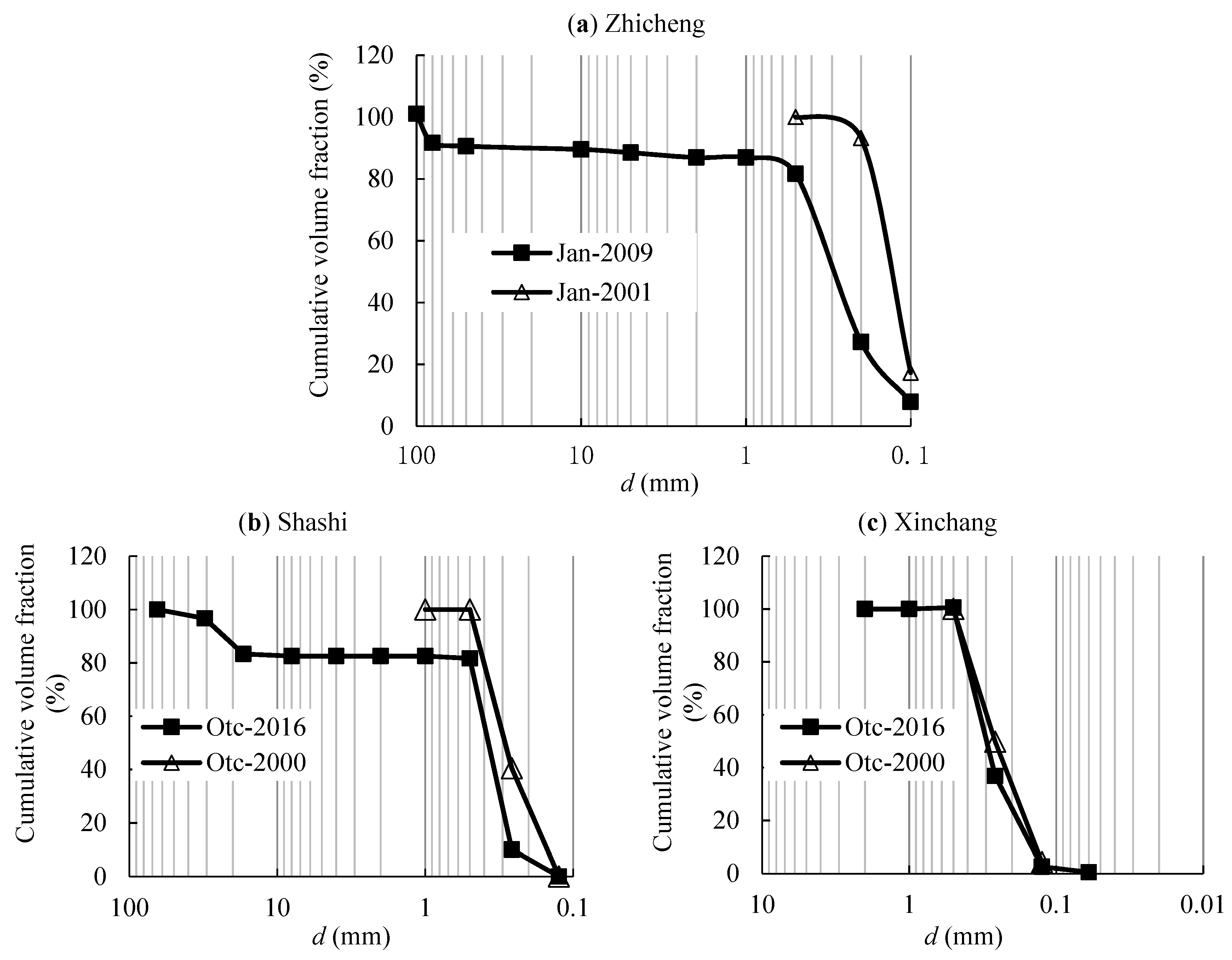
Figure 6.
Temporal variation of water runoff and SSL in the JJRR.

Figure 7.
Mass curves of anomalies of runoff and SSL at Zhicheng (a), Shashi (b), and Jianli (c) hydrological stations (1987–2014).
Figure 7.
Mass curves of anomalies of runoff and SSL at Zhicheng (a), Shashi (b), and Jianli (c) hydrological stations (1987–2014).
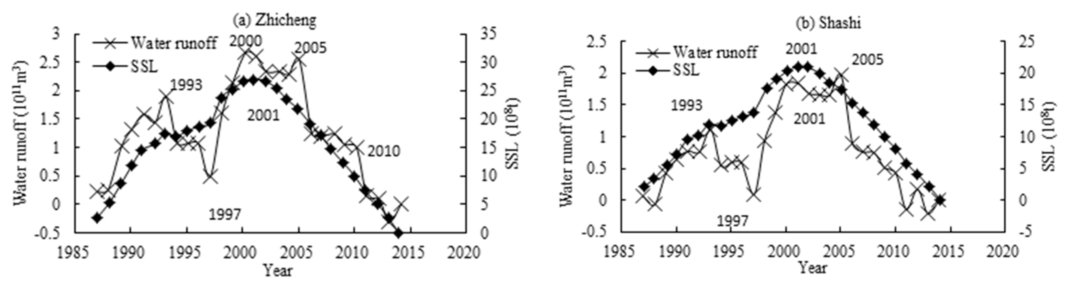

Figure 8.
Coefficients and exponents of sediment rating curves (a) for log(e) and (b) for f; solid lines are data drawn from Yang et al. [39].
Figure 8.
Coefficients and exponents of sediment rating curves (a) for log(e) and (b) for f; solid lines are data drawn from Yang et al. [39].
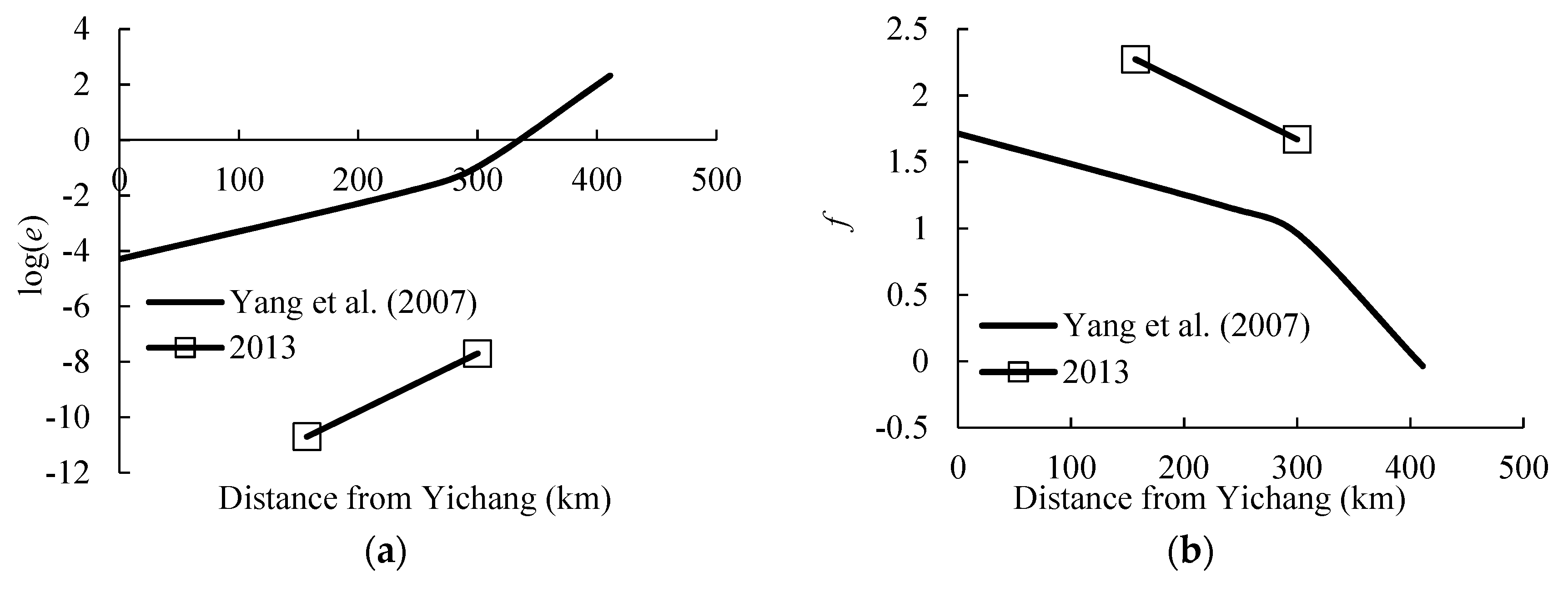
Figure 9.
Cumulative volume fractions of suspended sediment at 2016: (a) measured in July 2016 and (b) data measured in September 2016.
Figure 9.
Cumulative volume fractions of suspended sediment at 2016: (a) measured in July 2016 and (b) data measured in September 2016.

Figure 10.
Comparison between measured and calculated vertical profiles of suspended sediment concentration. Data in (a) were measured on 10 August 2011 at Shashi station, data in (b) were measured on 26 September 2013 at Shashi station, and data in (c) were measured on 27 November 2017 at Jianli station.
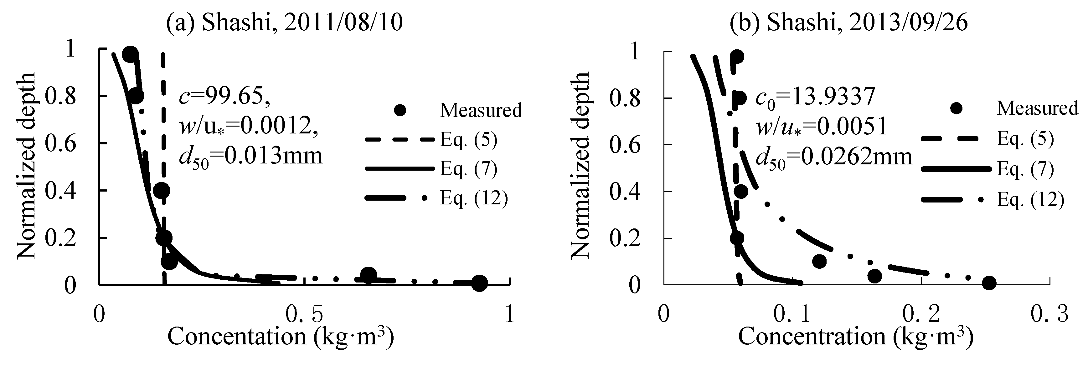
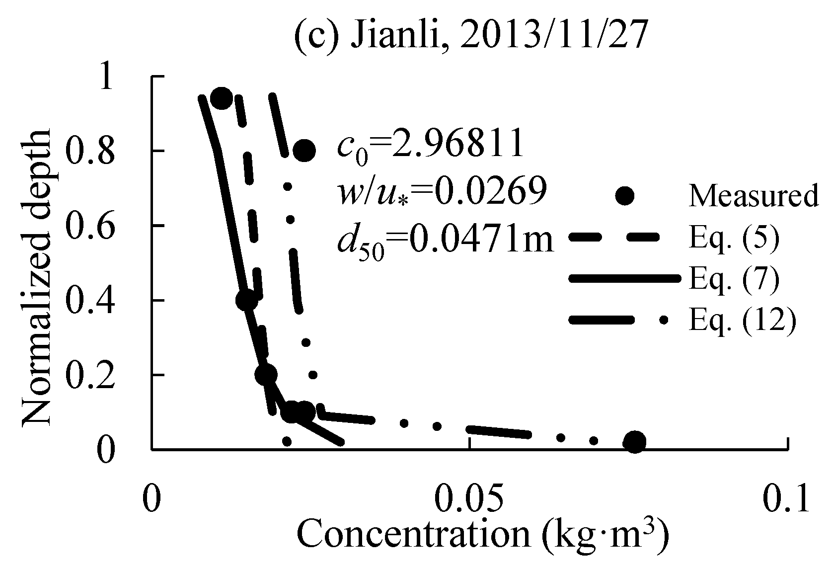
Figure 11.
Contribution of the near-bed load on sediment flux.

Table 1.
Statistics of data measured at the JJRR (following [17]).
Table 1.
Statistics of data measured at the JJRR (following [17]).
| Stations | Observation Year | No. of Verticals |
|---|---|---|
| Zhicheng | 1996, 1998, 2002 | 55 |
| Shashi | 1996, 1998, 2010, 2011, 2012, 2013 | 130 |
| Jianli | 1986, 1998, 2002, 2010, 2011, 2012, 2013 | 180 |
Table 2.
Statistical characteristics of vertical profiles.
| River Reach or Hydrological Station | Sa/Savg | Minimum Relative Depth (Reference Height a) | Water Depth (m) | (ω/u∗) | Mean Diameter (mm) | Vertical Averaged Concentration (kg·m−3) | Velocity (m·s−1) | Source | ||
|---|---|---|---|---|---|---|---|---|---|---|
| Maximum Value | Average Value | |||||||||
| Post-reservoir | Shashi | 15.05 | 3.22 | 0.0051 (0.1 m from river bed) | 2.09|19.70 | 0.16|108.89 | 0.0098|0.224 | 0.0052|1.29 | 0.42|2.12 | Field survey |
| Jianli | 14.45 | 4.89 | 0.0047 (0.1 m from river bed) | 2.13|21.2 | 0.13|76.15 | 0.0087|0.220 | 0.015|1.26 | 0.27|2.69 | ||
| Pre-reservoir | Zhicheng | 2.76 | 1.33 | 0.04 | 1.69|52.88 | | | 0.0052|0.0134 | 0.55|1.76 | | | |
| Shashi | 2.30 | 1.35 | 0.018 (0.4 m from river bed) | 4.3|22.6 | 0.08|1.34 | 0.0058|0.0265 | 0.188|1.99 | 0.08|1.34 | ||
| Jianli | 3.62 | 1.57 | 0.019 (0.4 m from river bed) | 3|21.3 | 0.024|12.12 | 0.0037|0.0699 | 0.26|1.71 | 0.17|2.62 | ||
| Changjiang Estuary | 4.33 | 0.044 | | | | | 0.009 | 0.11|0.83 | 0.24|2.04 | [30] | ||
| Oujiangkou and Taizhou sea area | 2.38 | 0.02 | | | | | | | | | | | [31] | ||
| Wuhan and Jiujiang River Reach | 1.32 | 0.19 | 10|25 | 0.007|0.036 | 0.003|0.01 | 0.01|0.1 | | | [32] | ||
| Silty Coast | 2.15 | 0.045 (0.012 m from river bed) | 0.14|1.95 | | | 0.12|0.33 | 1.50|5.30 | | | [33] | ||
Table 3.
Characteristics of vertical profiles with positive and negative gradations at Shashi and Jianli hydrological stations.
Table 3.
Characteristics of vertical profiles with positive and negative gradations at Shashi and Jianli hydrological stations.
| Stations | Post-Reservoir | Pre-Reservoir | ||||
|---|---|---|---|---|---|---|
| Negative | Positive | Negative | Positive | |||
| No. of Verticals | D50 (mm) | No. of Verticals | D50 (mm) | No. of Verticals | No. of Verticals | |
| Shashi | 50 | 0.01–0.06 | 45 | 0.03–0.07 | 29 | 7 |
| Jianli | 76 | 0.06–0.10 | 29 | 0.06–0.10 | 60 | 15 |
Table 4.
Contribution by various factors on sediment flux 1.
| River Reach | Total Sediment Flux 2 (104 m3) | Contribution by Near-Bed Concentration | Contribution by Other Factors | ||
|---|---|---|---|---|---|
| Sediment Flux (104 m3) | Ratio (%) | Sediment Flux (104 m3) | Ratio (%) | ||
| Yichang–Zhicheng | 10,275 | 1267 | 12.33 | 2047 | 19.92 |
| Zhicheng–Shashi | 11,242 | 980 | 8.72 | 4317 | 38.40 |
| Shashi–Jianli | 12,840 | 2303 | 17.94 | 1494 | 11.64 |
© 2018 by the authors. Licensee MDPI, Basel, Switzerland. This article is an open access article distributed under the terms and conditions of the Creative Commons Attribution (CC BY) license (http://creativecommons.org/licenses/by/4.0/).
Share and Cite
MDPI and ACS Style
He, L.; Chen, D.; Zhang, S.; Liu, M.; Duan, G. Evaluating Regime Change of Sediment Transport in the Jingjiang River Reach, Yangtze River, China. Water 2018, 10, 329. https://doi.org/10.3390/w10030329
AMA Style
He L, Chen D, Zhang S, Liu M, Duan G. Evaluating Regime Change of Sediment Transport in the Jingjiang River Reach, Yangtze River, China. Water. 2018; 10(3):329. https://doi.org/10.3390/w10030329
Chicago/Turabian StyleHe, Li, Dong Chen, Shiyan Zhang, Meng Liu, and Guanglei Duan. 2018. "Evaluating Regime Change of Sediment Transport in the Jingjiang River Reach, Yangtze River, China" Water 10, no. 3: 329. https://doi.org/10.3390/w10030329
Note that from the first issue of 2016, this journal uses article numbers instead of page numbers. See further details here.