Article

Real-Time Flood Control by Tree-Based Model Predictive Control Including Forecast Uncertainty: A Case Study Reservoir in Turkey

by
Gökçen Uysal
1,2,*,
Rodolfo Alvarado-Montero
1,3,
Dirk Schwanenberg
1,4 and
Aynur Şensoy
2
1
Institute of Hydraulic Engineering and Water Resources Management, University of Duisburg-Essen, 45141 Essen, Germany
2
Department of Civil Engineering, Anadolu University, 26555 Eskişehir, Turkey
3
Deltares, Operational Water Management, Deltares, Rotterdamseweg 185, 26 MH Delft, The Netherlands
4
KISTERS AG, Business Unit, Pascalstraße, 52076 Aachen, Germany
*
Author to whom correspondence should be addressed.
Water 2018, 10(3), 340; https://doi.org/10.3390/w10030340
Submission received: 18 December 2017 / Revised: 8 March 2018 / Accepted: 9 March 2018 / Published: 19 March 2018
(This article belongs to the Special Issue Adaptive Catchment Management and Reservoir Operation)

Abstract

:
Optimal control of reservoirs is a challenging task due to conflicting objectives, complex system structure, and uncertainties in the system. Real time control decisions suffer from streamflow forecast uncertainty. This study aims to use Probabilistic Streamflow Forecasts (PSFs) having a lead-time up to 48 h as input for the recurrent reservoir operation problem. A related technique for decision making is multi-stage stochastic optimization using scenario trees, referred to as Tree-based Model Predictive Control (TB-MPC). Deterministic Streamflow Forecasts (DSFs) are provided by applying random perturbations on perfect data. PSFs are synthetically generated from DSFs by a new approach which explicitly presents dynamic uncertainty evolution. We assessed different variables in the generation of stochasticity and compared the results using different scenarios. The developed real-time hourly flood control was applied to a test case which had limited reservoir storage and restricted downstream condition. According to hindcasting closed-loop experiment results, TB-MPC outperforms the deterministic counterpart in terms of decreased downstream flood risk according to different independent forecast scenarios. TB-MPC was also tested considering different number of tree branches, forecast horizons, and different inflow conditions. We conclude that using synthetic PSFs in TB-MPC can provide more robust solutions against forecast uncertainty by resolution of uncertainty in trees.

1. Introduction

Reservoirs are one of the main components of integrated water resources systems. Their control poses a challenging problem, since it must cope with different conflicting objectives as water supply, hydropower, and flood control [1,2,3,4,5]. Operating with guide curves is a common practice in typical reservoir operation [6,7,8]. These operating strategies however, rely on long term records that can filter and underestimate extreme events such as drought and flood conditions [9]. Flood events strain reservoir operators to refill and keep maximum water levels. In response to short-term fluctuations, the operators need to anticipate actions and release the excess amount of water in order to have sufficient flood storage volume in the reservoir [10]. However, the storage after the event must be recovered in order to satisfy water supply during the following dry season [11]. Therefore, flood control and water conservation require careful planned strategies for short-term operation. On the other hand, system optimization on this time scale becomes more complex due to the high-dimensionality, non-linearity of the system, and dynamic structure of the control process.
In general, a reservoir operation is assumed to be a dynamic system in which the future states are a function of the current states. Throughout optimization of sequential decision processes, Dynamic Programming (DP) developed by Bellman [12] is an important milestone. The main problem can be divided into sub-problems, separately solved successively over each stage to get an overall optimum solution. Later, researchers contributed on this technique in different aspects such as using sampling stochastic DP, incremental DP, stochastic dual DP [13,14,15]. Though the solution is well suited for highly nonlinear, nonconvex problems, the main difficulty arises with the so-called “curse of dimensionality”. This means more (exponentially growing) computational time with increasing dimensions of states, decisions, and disturbances [12,16].
Operation of the reservoir system is an optimal control problem, thus an alternative solution is proposed by adapting Model Predictive Control (MPC, also known as Receding Horizon Control) [17]. The concept has been tested in different application areas such as rivers, reservoirs, and irrigation canals [18,19,20] in water resources management. The system is optimized for a forecast horizon by solving an open-loop control problem simultaneously in every time step, then only the first time step control value of the computed sequence is applied and the rest are discarded. At the next step, system states are updated and the process is repeated again. This feedback mechanism is called closed-loop optimization. In the real-world, the reservoir system is operated according to forecast based control decisions, but updated to the realization of the disturbance (inflows). Thus, in the study closed-loop experiments are preferred due to the feedback mechanism to mimic the real-world reservoir operation decisions with respect to open-loop experiments.
MPC requires prediction of disturbance in the real-time control of a water structure, but streamflow forecasts always bring along forecast uncertainty. In real-time forecasting applications, forecasts can be biased and tend to over- or underestimate the actual streamflow [21] and it is hard to fully avoid this [10]. In practice, there are several sources of uncertainty that reduce the accuracy of peak flow estimation. Essentially, these are the hydrological forecast model structure [22], model external forcing e.g., precipitation [23,24], model parameters [25], and initial conditions [26].
Although it is not possible to eliminate all types of uncertainties, one solution might be the consideration of forecast uncertainty using ensemble forecasts in short-term operation. Labadie [16] sorted the hindrances of reservoir system operations, among them he emphasized the need to incorporate uncertainty and risk issues in optimization models. Recently, different researchers showed how probabilistic flood forecasts are more robust and effective than the traditional deterministic ones; correspondingly systems are improved by models that quantify forecast uncertainty [27,28,29].
In short-term management, Numerical Weather Prediction (NWP) based Ensemble Prediction Systems (EPS) can provide probabilistic streamflow forecasts. The idea behind it is to represent future states of the atmosphere by perturbing the initial conditions (uncertainty). Uncertainty becomes much larger when managing small basins and small rivers [30]. In the case of non-availability or inadequacy of the numerical weather forecast data, synthetic streamflow generation is a common practice for reservoir simulation and optimization studies especially in hypothetical studies [28]. There are various approaches to produce synthetic data e.g., the Thomas-Fiering model [28], Fractional Gaussian noise model [31], artificial neural network [32] or hybrid models [33]. Among them, only a limited number of studies [28,31] demonstrate the forecast uncertainty evolution process such that future periods have larger uncertainty and that there is a correlation between uncertainties.
While MPC seeks optimum trajectories based on a single disturbance, i.e., the inflow into a reservoir, its stochastic counterparts try to find an optimum solution for the entire ensemble and incorporate forecast uncertainty. However, this might yield an infeasible solution due to the burden of multiple disturbance in combination with hard constraints. An innovative technique to deliberate ensemble forecasts with an adaptive control is proposed as Tree-Based MPC (TB-MPC) [34]. This approach reduces the number of ensemble members by its tree generation algorithms using all trajectories and then proper problem formulation is set by Multi-Stage Stochastic Programming. The method is relatively new in reservoir operation [34,35,36,37], especially closed-loop hindcasting experiments and its assessment is quite rare [24] in the literature.
This paper demonstrates a real-time flood control in consideration of streamflow forecast uncertainty especially for limited storage multi-purpose reservoirs using synthetic ensemble inflows and the mass-conservative TB-MPC method. While we focus on the trade-off between flood risks and water conservation benefits, its implementations into the test case follow: (1) development of a novel Probabilistic Streamflow Forecasts (PSFs) method to produce ensemble inflows, (2) the configuration of an hourly (deterministic and stochastic) predictive reservoir optimization model, (3) testing of different PSF scenarios in closed-loop hindcasting mode in comparison with deterministic counterparts (perfect data and Deterministic Streamflow Forecasts, DSF) and (4) the assessment of TB-MPC model features considering different number of tree branches, different inflow conditions, and different forecast horizons in the area of interest.
In this study, the methodology is applied to the Yuvacik dam reservoir, fed by a catchment area of 258 km2 and located in Turkey, owing to its challenging operation due to downstream flow constraints. The reservoir serves as a main water supply for Kocaeli province. First, a hydro-meteorological rule based decision support system is developed for daily and hourly operation [38]. Later, it is shown that underestimated daily inflow forecasts during a flood event operation in critical reservoir level may result in underestimated spillage releases when using deterministic MPC [39]. Therefore, the case establishes a precedent for similar relatively small reservoirs with multi-purpose operational characteristics. At this point, this paper complements deterministic methods by PSF integrated TB-MPC including forecast uncertainty.

2. Materials and Methods

Hindcasting experiments are the representation of a real-time system by an iterative process: (i) MPC anticipates required spillages with the optimization model for a given time length (so-called forecast horizon). (ii) The reservoir simulation model updates with actual inflows and anticipated spillages from step (i) to find updated forebay elevations. (iii) This process is repeated every hour (so-called receding horizon) until the whole hindcasting period (96 h in this study) has been completed. The general methodology is outlined in Figure 1. We apply closed-loop hindcasting experiments by the following three modes:
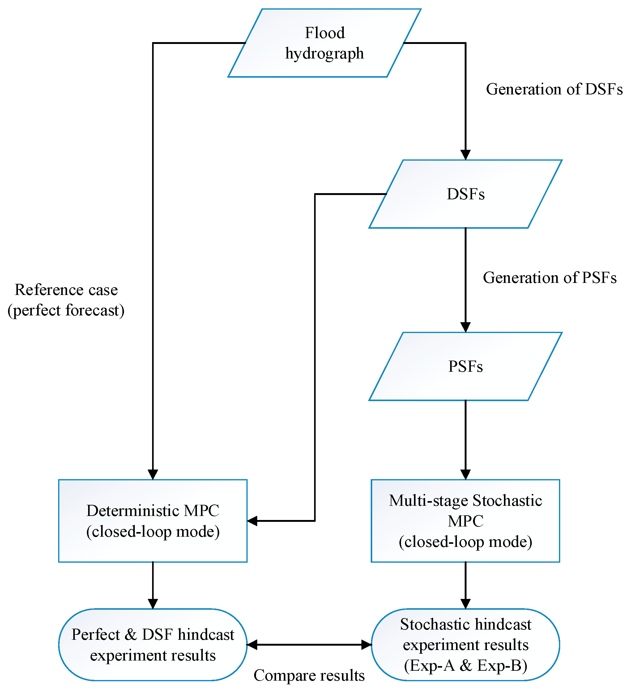
  • Perfect Hindcast Experiments: The flood hydrograph corresponding to a 100 years return period (Q100) of the basin is utilized as perfect forecast data in deterministic MPC. This represents the best solution since it exhibits the optimized releases and forebay elevations under perfect knowledge of the future inflows, and it is evaluated as reference case for comparative analyses with forecast based models.
  • Deterministic Hindcast Experiments: This represents the skill of single value DSF evaluation by deterministic MPC. Randomly perturbed inflows in each receding horizon are employed in deterministic MPC mode. The random perturbation having a forecast horizon up to 48 h is updated in each hour.
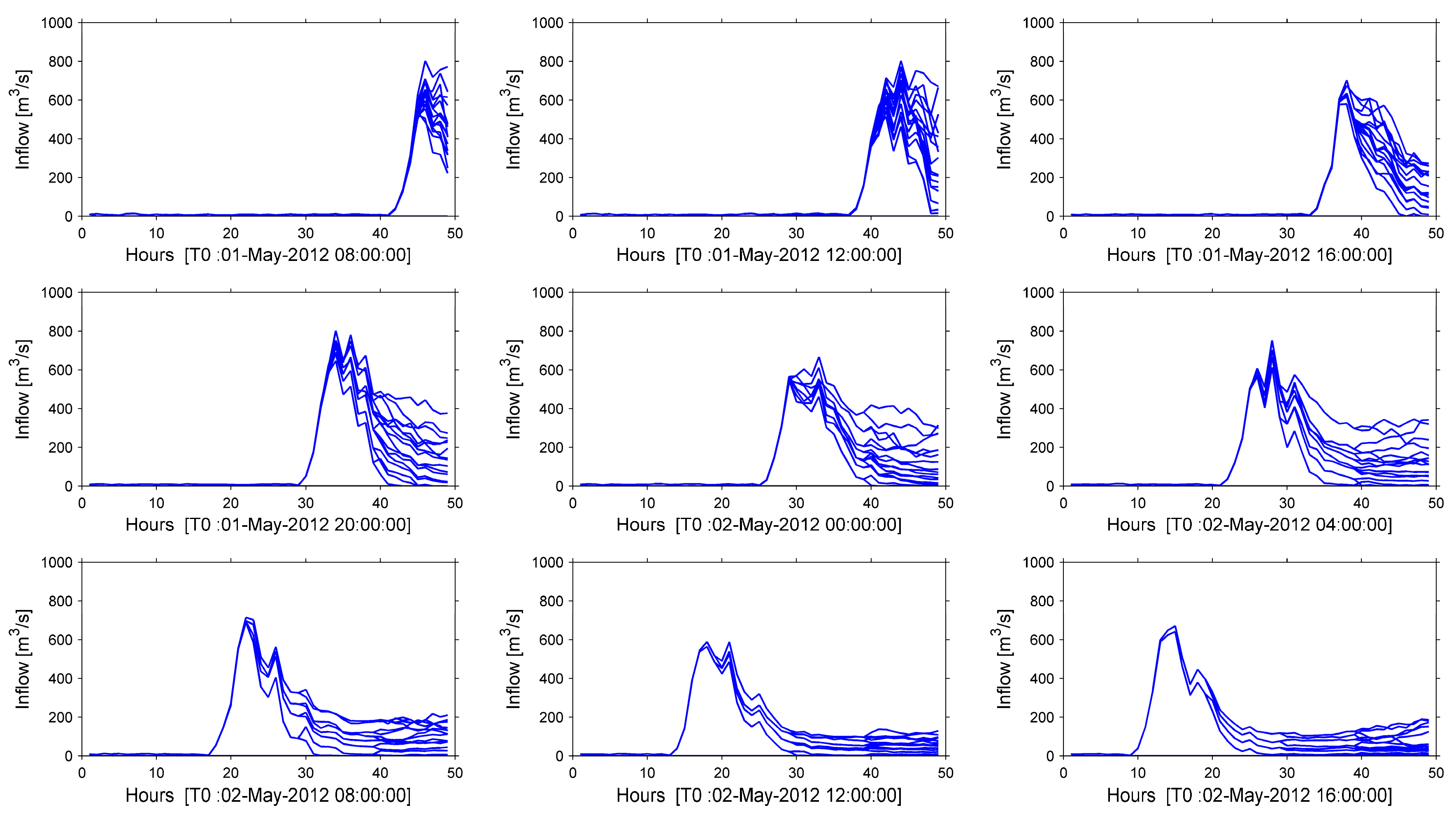
  • Probabilistic Hindcast Experiments: This represents the skill of ensemble PSF evaluation by multi-stage stochastic TB-MPC. Synthetically generated ensemble inflows in each receding horizon are employed in stochastic MPC mode (Exp-A). This provides forecast uncertainty consideration in the application. Moreover, features of TB-MPC are investigated with selection of different forecast horizons, tree branching numbers, and different inflow conditions (Exp-B).

2.1. Deterministic and Probabilistic Synthetic Streamflow Generation
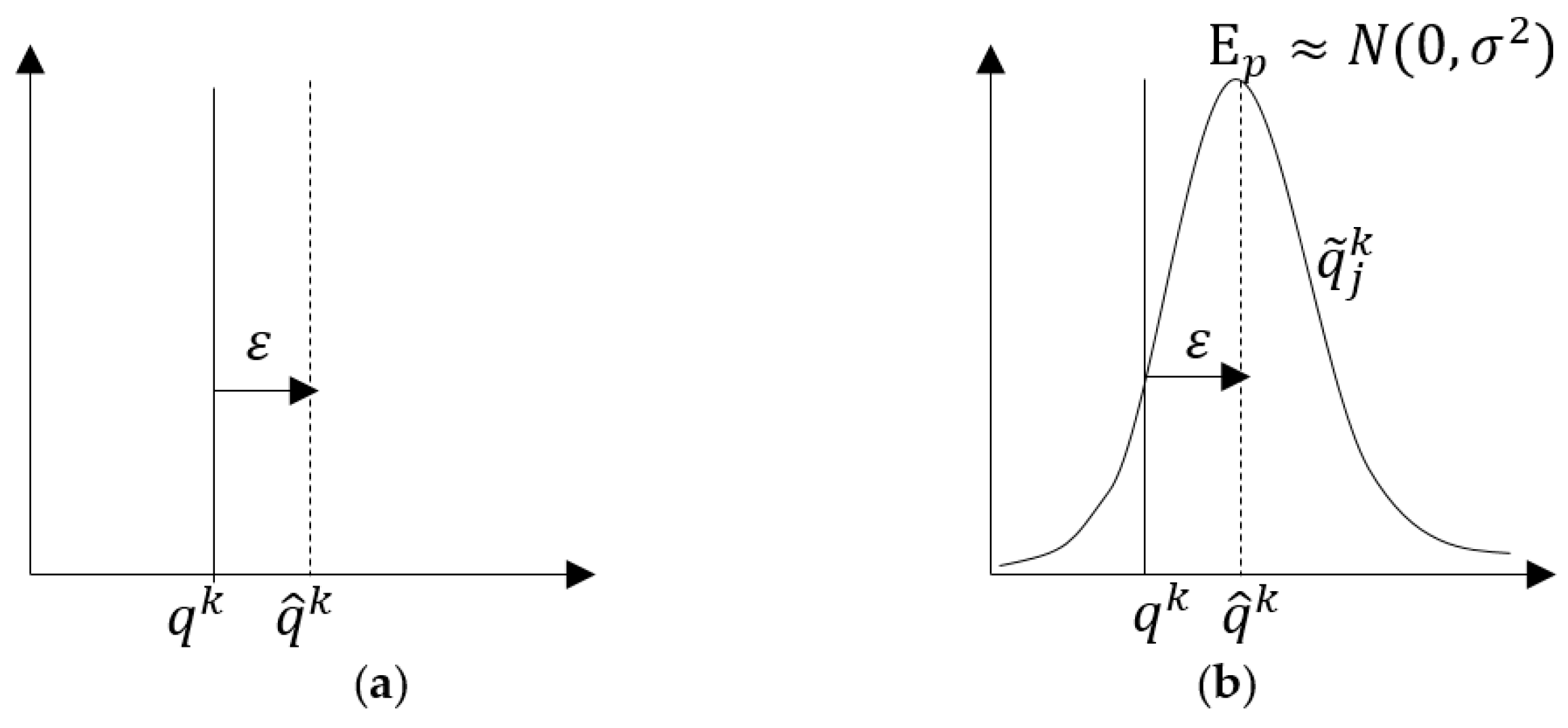
Since forecast inflows include uncertainties, they can be represented by the relative inflow forecasting error [10]. In this paper, we refer to them as DSF scenarios which are perturbed from original flood hydrographs. While the DSF sequence is a single value, the PSFs are generated by applying a dispersion around the DSF with a specified probability distribution (Figure 2). They are eventually repeated in each time step (depending on selected receding horizon) to mimic a dynamic real-time system.
DSF is represented by random perturbation using relative inflow forecasting error ( ε ).
ε k = q ^ k q k   q k
D S F :   q ^ k = q k ( 1 + ε k )
where ε , q ^ , q stands for relative inflow forecasting error, forecasted inflows, observed inflows, respectively over a forecast horizon represented by k = 1 , , N time instants.
Even though a range of relative inflow forecasting errors can be detected in the literature [40], acceptable ε during a flood forecasting is within a 0.15–0.30 interval in real-world hydrological forecasting studies [4,10,41]. These studies cover different project scales and climatology. In this study ε values are randomly selected from uniform distribution and range between −0.3 and 0.3 to generate individual DSF values from observed inflows. Also, ε values change for each k time instant.
We produce a set of synthetized members (ensembles, PSF) that are spread around single valued DSF. Conventionally, uncertainty is defined by relative standard error which is expected to be independent (also referred as white noise), usually Gaussian with zero-mean. Therefore, the error pdf is assumed to be Ε p N ( 0 , σ 2 ) for all time steps [21,28,42,43].
We introduced a forecast evolution process which is similar to that of Zhao et al. [28] with increasing forecast uncertainty through the forecast horizon. Our implementation of correlation between forecast errors however, is defined by the algorithm below. Synthetic PSFs are generated as an empirical conditional distribution of the perturbed DSF. In other words, they have certain mean ( μ ) from DSF and relative standard error ( σ ^ = σ μ ), considered as an uncertainty level.
We consider the following notation of probabilistic scenario in an ensemble forecast (PSF) matrix as:
P S F = [ q ˜ 1 1 q ˜ 2 1 q ˜ j 1 q ˜ M 1 q ˜ 1 2 q ˜ 2 2 q ˜ j 2 q ˜ M 2 q ˜ 1 k q ˜ 2 k q ˜ j k q ˜ M k q ˜ 1 N q ˜ 2 N q ˜ j N q ˜ M N ]
where N denotes the length of forecast data (so-called forecast lead-time), M denotes the number of ensemble members, q ˜ j k denotes an arbitrary ensemble member in matrix, and k , j correspond to lead-time and ensemble member indexes, respectively
The procedure to generate synthetic PSFs is accomplished mainly in two successive steps:
  • In the initial time step, PSF ( q ˜ j 1 ) members are generated as:
    q ˜ j k = N ~ ( q ^ k , q ^ k σ ^ k ) ,   k = 1   &   j = 1 , 2 , , M
  • The PSF should be correlated with previous members, therefore, the differences between successive DSF values (referred to k time instants for the same DSF sequence) are calculated, then normally distributed errors having mean and standard error from the previous time step are generated and added to the differences. Maximum function is added in order to eliminate negative values, and the remaining PSF members ( q ˜ ) are formulated as:
    q ˜ j k = ( q ^ k q ^ k 1 ) + max ( N ~ ( q ^ k 1 , q ^ k 1 σ ^ k ) , 0 ) k = 2 , , N   &   j = 1 , 2 , , M
According to intuition, a longer forecast lead-time results in a less reliable forecast. The level of forecast uncertainty (in terms of relative standard error) is assumed to be the same for all members but increasing towards the forecast horizon:
σ ^ k 1 σ ^ k σ ^ k + 1
Uncertainty in the precipitation is typically much greater (even the largest source of uncertainty from input data) compared to the other meteorological variables [44]. Since higher precipitation leads to higher discharge data, total uncertainty of the forecast chain is expected to be higher during rainfall events, and less during no rain condition. Therefore, this condition is considered in the application by updated relative standard errors depending on DSF values as:
σ ^ k = { σ ^ k = σ ^ k 1 i f q ^ k q ^ k 1 σ ^ k > σ ^ k 1 i f q ^ k > q ^ k 1 }
In the application, a cumulative forecast uncertainty (relative standard error of the final time step, σ ^ N ) is selected beforehand and incremental standard error values are calculated for each time instant. This is a posteriori information based on trial-and-error by the assessment of forecast uncertainty.

2.2. Deterministic Model Predictive Control (MPC)

Contrary to feedback controls where control actions are determined with the current state of the system, MPC takes the future state of the system into account. MPC is commonly implemented by having several components in a receding horizon strategy. These components are a system description (model), a set of disturbances (water inflow into the system, water extractions etc.), objective and physical or operational constraints to represent physical operational management objectives and constraints of the system. Deterministic MPC considers a discrete time-dynamic system according to
x k = f ( x k 1 , x k , u k , d k )
y k = g ( x k , u k , d k )
where x , y , u , d are, respectively, the state, dependent variable (output), control, and disturbance vectors, f ( . ) and g ( . ) are linear or non-linear, time-variant vector functions representing an arbitrary water resources model [45]. If being applied in MPC, Equations (8) and (9) are used for predicting future trajectories of the state x and dependent variable y over a finite time horizon represented by k = 1 , , N time instants, in order to determine the optimal set of control variables u by an optimization algorithm. Under the assumption of knowing the realization of the disturbance d k over the time horizon N , for example the inflows into the reservoir system { d k } 1 N , the simultaneous (or collocated) MPC [45] becomes:
m i n u , x { 0 , , T } k = 1 N 1 J ( x k , u k , d k ) + E ( x N , u N , d k )
s . t . : h ( x k , y k , u k , d k ) 0 , k = 1 , , N
x k f ( x k 1 , x k , u k , d k ) = 0
where J ( ) is a cost function associated with each state transition, E ( ) is an additional cost function related to the final state condition, and h ( ) are hard constraints on control variables and states, respectively. It receives a single disturbance vector, so that it might be either an observed or deterministic forecast. In a simultaneous or collocated mode, the related process model (Equation (8)) becomes an equality constraint of the optimization problem at dedicated time steps in Equation (12) [46]. The optimization problem is solved using an efficient gradient-based optimizer such as the nonlinear optimizers IPOPT [47] with MA27 solver of the HSL library in combination with adjoint modeling. Adjoint modeling is essential for the efficient computation of the derivative of the objective function with respect to the controlled variables ( d J = d ( x k , u k , d k ) / d u k ). The model itself is implemented in RTC-Tools [45].

2.3. Multi-Stage Stochastic Tree-Based MPC (TB-MPC)

In this part, the deterministic model is extended to a multi-stage stochastic optimization model. The stochastic nature of inflows is reflected by a probabilistic forecasts ensemble, d j k , where j denotes the ensemble index ( j = 1 , , M ) and k denotes the time instant ( k = 1 , , N ). Hence, Equation (10) is rearranged for J and E , then it becomes the probability-weighted sum of the objective function terms of the individual ensemble. The formula is shown below as:
m i n u , x { 0 , , T } j = 1 M p j k = 1 N 1 J ( x j k , u j k , d j k ) + E ( x j N , u j N , d j N )
where p j stands for the probability of the ensemble member (equal for each one), M stands for the number of the ensembles.
The key factor of the approach depends on the control variable ( u j k ) definition for setting up of a stochastic optimization problem due to the limitation of the usable storage. A simple way would be to find the control trajectory which is optimal for the whole ensemble (on average, worst case, chance constrained, etc.). In case of an average definition, it might give feasible solutions on consideration of the ensemble having small variations. However, if the operation of the reservoir system is highly constrained due to a limitation of storage, the solution of the optimization can be dominated by these constraints or it becomes infeasible.
To avoid this problem, multi-stage stochastic optimization is proposed and successfully applied using scenario trees for disturbance, states, and control trajectories [34,48]. Thus, the approach becomes adaptive, the control trajectory does take into account the resolution of uncertainty. This means uncertainty is gradually resolved by showing tree branches at specific time instants along the forecast horizon. While scenario reduction is employed in various ways and represented by a tree nodal partition matrix P ( j , k ) M x N , a recently proposed novel mass conservative approach which keeps the probability-weighted sum of a quantity of the original ensemble is used in this study. Details are available in [24,37]. We present the first implementation of the TB-MPC in application to a synthetically generated ensemble streamflow forecast for a limited storage multi-purpose reservoir under flood case.

3. A Real World Test Case and Model Set-Up
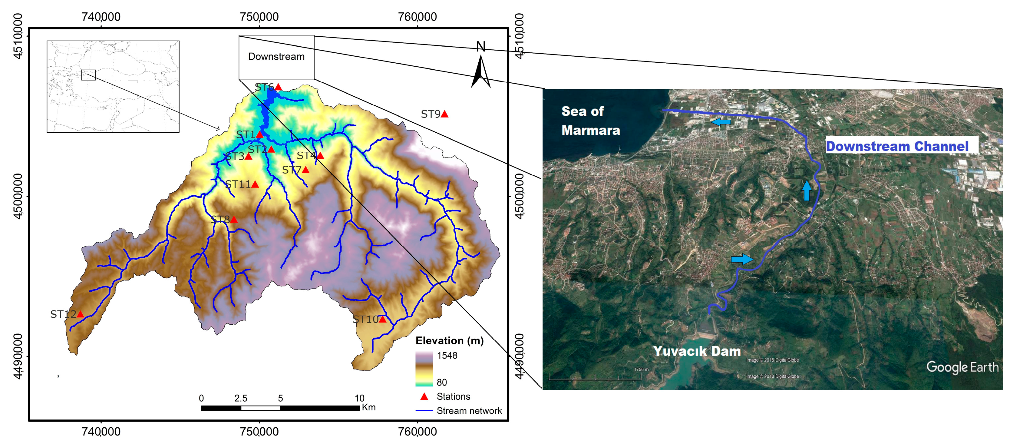
3.1. Study Area

The proposed methodology was tested in the Yuvacik Dam reservoir, with a 258 km2 catchment area, located in the east part of Marmara Region, Turkey (Figure 3). The earth-filled dam was constructed in 1999 for the water supply of Kocaeli city. An annual 142 hm3 of drinking, domestic and industrial water for 1.5 million inhabitants should be supplied. The relatively limited reservoir has an active storage capacity of approximately 51.2 hm3 at maximum operating level of 169.3 m whereas 169.8 m is the maximum water level. The spillway is controlled by four radial gates. It should be noted that while a volume of 36.60 hm3 is stored between minimum operation level of 112.50 m and spillway crest elevation of 159.95 m, a volume of 14.60 hm3 is kept above spillway crest elevation and behind the radial gates. On the other hand, a Dam Management System (DMS) which has been developed as a part of a Supervisory Control and Data Acquisition (SCADA) system by the reservoir operators provides data collection and transmission from automatic gauges.

3.2. MPC Inputs

The maximum amount of water to be released during daily operation is set as 100 m3/s by the regional water authority taking the drainage discharge conditions of the downstream canal and lateral flows into consideration. The main reason for that is a 12 km long downstream reach that passes from a narrow valley near a rural district and flows into the Marmara Sea after a sharp curvature by a manmade channel next to industrial and urban areas. The dam is built to protect the downstream region against extreme flood events, and the maximum spillway release is set to 200 m3/s during hourly flood control. This value is the maximum allowable flood limit without severe damage in the downstream. The operation of the dam is multi-purpose subject to two main objectives: (i) water supply and (ii) flood control.
Since available data are insufficient to precisely assess extreme events [49], design flood hydrographs are generally derived based on maximum instantaneous records at the dam site, selected probability distributions using several parameters [50,51], and considered to be representative of extreme conditions expected in the future. In the Yuvacik catchment, the annual peak flow values over 19 years were statistically analyzed and it was detected that the series is in line with the Gumbel dispersion function according to the DSI (State Hydraulic Works, the main governmental water organization in Turkey) report [52]. The peak flow flood values are derived for different return periods (Table 1).
The study adopted a 24 hourly flood hydrograph having an expected occurrence of 100 years that is utilized as a perfect streamflow forecast (Q100 flood hydrograph) in the main test application. The flood peak-occurrence time from the beginning is 6 h (i.e., the response time of the catchment to the rainfall event) and the peak flow corresponds to 597 m3/s. The total flood volume equals to 17.1 hm3. Being an extreme case, the peak flow of the selected flood hydrograph is three times greater than the downstream channel capacity (200 m3/s). The hindcasting experiments were conducted in an arbitrary year during a critical operation period (May) when the initial forebay elevation was high. The whole closed-loop hindcasting period covers 96 h, from [1-May-2012 00:00:00] to [4-May-2012 23:00:00]. It is assumed that a 24-h long flood hydrograph occurs between [3-May-2012 00:00:00] and [3-May-2012 23:00:00]. Hourly forecast data are produced for 48 h lead-time. This means that in each 1 h, 48-h long DSF data (with 1 member) and 48-h long PSF data (with M = 50 ensemble members) are generated throughout the whole hindcasting period. Given the lack of probabilistic hydrological forecasts for this case study, we decided to recreate the stochasticity by assuming a normally distributed noise around the deterministic forecast. This in fact becomes an innovation on its own in the paper, since an objective approach has not been reported in the literature before. Although it was desired to increase the number of PSF members in order to cover much more possibilities, this ended up with the reverse situation in the optimization model due to the high-dimensional data space. Different ensemble sizes were also tried in the control model, and it was observed that increasing member number estimates higher uncertainty range, 50 members are considered to provide enough spread to capture the major uncertainties in the forecasts.
In this study, DSFs with error range between −0.3 and 0.3 and PSFs with final relative standard error ( σ ^ 48 = 0.2 ) are depicted with three different randomized scenarios (Sce-Q100a, Sce-Q100b and Sce-Q100c). Here, a scenario corresponds to randomly generated and independent forecasting data sets (both DSFs and PSFs) to be employed in the same hindcasting period. In each scenario, randomly perturbed DSFs from perfect data are produced in each hour for a given lead-time and an error interval. Then, similarly (in each scenario and in each hour), ensemble PSFs are produced from the mother DSFs with a given uncertainty. Since the generated streamflows are produced in each hour, the receding horizon is always set to one hour in all deterministic and stochastic MPC hindcasting experiments. In terms of operational point of view, the control trajectory changes at each time step and is not a fixed one for the complete event (it changes depending on the forecast and its uncertainty, as well as the forecast horizon).
As explanatory example from two scenarios (Sce-Q100a and Sce-Q100b) is shown in Figure 4 for a lead-time of 48 h. Fifty members are generated for PSFs, but only two members (min and max values) are given in the figure to show the uncertainty ranges (referred to uncertainty band). In the figure, [T0] corresponds to “time zero” namely the starting time of the optimization. Two time instants [T0: 01-May-2012 12:00:00] (Figure 4a) and [T0: 01-May-2012 13:00:00] (Figure 4b) are exampled here, but the process is dynamically repeated in each one hour throughout the hindcasting period in closed-loop experiments for each scenario. Finally, each scenario is composed of all generated 96 forecast sequences (both in DSFs and their PSFs) having a 48 h lead-time in the hindcasting period.
Different inflow conditions such as Q25 and Q50 (from Table 1) are also tested under Section 4.3.3. Characteristics of the PSF scenarios are presented with the performance assessment by using a mean Continuous Ranked Probability Score (CRPS) which generalizes the Mean Absolute Error (MAE) in the case of probabilistic forecasts (Supplementary Figure S1). Mean CRPS summarizes the quality of a probability forecast into a number by comparing the integrated square difference between the cumulative distribution function of forecasts and observations [24]. According to that, mean CRPS increases with forecast lead-time, while each scenario shows a different performance. The scenario number is not critical in the study because the focal idea is to develop an objective approach for stochasticity of the flows, to use them in stochastic optimization set-up and to compare the results with a deterministic equivalent. Thus, scenarios can be deliberated as different source based forecast data sets.
An example of generated forecast data sets (Sce-Q100a) is given for different time steps shown by T0 in Figure 5. Similarly, [T0] corresponds to “time zero” namely the starting time of the optimization in the figure. The red dashed line shows DSFs which are derived from a perfect forecast by 30% random noise. Synthesized PSF data are shown in gray ink. While generating PSF, updated forecast data have “different starting time” and “different duration to the peak flow” which affect the uncertainty band in the end. For example, the starting time of the 01-May-2012 20:00:00 (fourth panel) and 02-May-2012 00:00:00 (fifth panel) have less duration to peak flow, thus they have higher dispersion at peak flow compared to the last panel and subsequently uncertainty is kept high in the falling limb in the fourth and fifth panels. However moving forward in time, the duration to peak flow at T0 decreases, so that the relative standard error cannot increase too much due to the flow condition. That is the reason why the last panel has less spread in the end. It is directly related to the approach used to generate the ensembles.
Contrary imperfect data (DSFs and PSFs), perfect forecast (shown in Figure 5 as a black line) is a single chain and utilized in the initial MPC hindcasting experiment. This test allows the performance of the developed real-time reservoir system control model to be assessed without forecast uncertainty; as a result a sufficiently long forecast horizon is decided before starting imperfect forecast tests. During TB-MPC hindcasting experiments, PSF data are converted to trees depending on the selected branch numbers. Hereby, previously generated forecast data (from Sce-Q100a) PSFs with 50 members (Figure 5) are transformed into optimization tree inflows with 16 branches (members) in Figure 6. Thereby, the number of generated PSF data are limited by this reduction, but still capture the major uncertainty, and the tree is used in the optimization algorithm.
Assessment of an effective reservoir operation in the short term is done by quantifying the minimization of downstream damage, the dam safety and maximization of the forebay elevation at the end of the flood event [53]. Similarly, four objective criteria are used in this study to test the experiments. These are:
  • Forebay elevation at the end of a flood event: Forebay elevation should be same at the end of a flood event in order to provide long term water supply targets,
  • Flooding threshold value: Spillway discharges should be less than channel capacity, thus this is considered as the flooding threshold value and the maximum discharge at the dam outlet is checked,
  • Total flood volume at the downstream area: The cumulative volume of the released flood water (only above the maximum flood limit of 200 m3/s) should be zero for the best flood management,
  • Flood storage index (FSI): It is essential to have enough flood pool in the reservoir to attenuate the hourly extremes. To measure this, FSI is defined by the ratio of the total effective flood storage over the total volume of storage corresponding to Flood Control Levels (FCLs) [4] as shown in Equations (14) and (15) . The reservoir level should be kept at FCL as suggested to reserve space for flood attenuation. FSI ranges between zero and one. While zero indicates the reservoir level is always kept above FCL, one indicates operation is totally based on FCL. Higher FSI ensures more reliable flood operation (under forecast uncertainty) by having a high empty reservoir volume against flood risk.
    F S I f = k = 1 N v f k k = 1 N v F C L k
    v f k = { v a c t k   i f   v k v F C L k v F C L k   i f   v k > v F C L k f o r   k = 1 , 2 , N
where v f k is the effective flood storage, v F C L k is the storage corresponding to FCL, v a c t k is the actual volume of the flood control pool; v k is the current storage by k = 1 , , N time instants. If v k is below FCL, it is equal to the volume of the flood control pool; otherwise, it is the actual available storage.
While the “flooding threshold value” gives the maximum instantaneous damage in the downstream, “total flood volume at downstream area” reflects the cumulative total penalty from the target set point of operational constraint within a hindcast period. It is also important to note that the perfect data based model results neglect uncertainty completely and serve as reference. Any deviation from these results objectively presents the inefficiency of the DSF and PSF based model results.

3.3. Model Set-Up

The reservoir model is based on the continuity equation for the reservoir. The water balance equation for a single reservoir can be arranged as:
s k = s k 1 + Δ t ( Q I k Q S k Q W S k )
where, s is the storage volume (m3), Δ t is the time difference between k t h and ( k 1 ) t h time steps, Q I , Q s , and Q W S are the reservoir inflows, spillway flow and water supply (m3/s), respectively. Also, forebay elevation, f b could be computed by:
f b k = f l s ( s k )
where f s l is a piecewise-linear level-storage relation.
In order to satisfy physical conditions capacity curves, discharge limits, and boundary elevations are introduced in constraints.

3.4. Physical and Operational Constraints

The constraints that form the equalities and inequalities are the continuity equation and the physical boundaries. The continuity equation ensures a consistent mass balance definition, accordingly residuum ( r k ) is introduced as an equality constraint and it must be zero as formulated below:
r k = s k s k 1 Δ t ( Q I k Q S k Q W S k ) = 0
The system’s physical limits should be met and they are defined as hard constraints. First, forebay level physical constraints are defined as:
f b m i n f b k f b m a x
where f b m i n is the minimum reservoir elevation and f b m a x is the maximum reservoir elevation. Beyond the operational targets, the spillway discharge flow should be within physical limits depending on its capacity curve and is defined as the constraint below:
Q s m i n Q s k Q s m a x k
Q s m a x k = f s d c ( f b k )
where Q s m i n is the minimum spillway flow and is set to zero and Q s m a x is the maximum allowable spillway flow and it is determined by the spillway discharge curve ( f s d c ) i.e., zero at spillway crest elevation and variable above elevations depending on the current forebay elevation (as a function of f b ).

3.5. Objective Function

An objective function determines the target of the operation by its terms. These terms are sometimes called soft constraints and an overall optimum of all terms is targeted. Optimization of a multi-purpose reservoir is aimed to mitigate flooding while maximizing water benefit or hydropower assets as its own objective function. Controlled variables are the forebay elevation and spillway discharges. The term sensitivity is set by the weights and the power of the equation. These weights are case-specific and depend on the significance of the soft constraints. For example, in this study higher penalizations are assigned for w 3 and w 4 in order to prevent downstream flooding and provide the long term water supply target, respectively. The weights are determined by a trial-and-error approach.
A reservoir having a limited capacity should include the terms below for hourly management:
  • Differences between optimized forebay elevation and maximum operating elevation are minimized in Equation (22),
  • Spillway discharges are minimized in Equation (23),
  • Spillway releases above a specified discharge (200 m3/s) are constrained in Equation (24). This has a high weight in order to prevent damage in the downstream,
  • The case of a set point for forebay elevation is given i.e., a variable guide curve (it is the same for each hour in a day) for long term targets [39], this term stands to minimize deviations from it in Equation (25),
  • Spillway discharges between two consecutive time steps are constrained by consideration of the mechanical gate operation efficiency (against wear and tear) in Equation (26).
    J 1 ( f b ) = w 1 k = 1 N ( f m a x f b k )
    J 2 ( Q s ) = w 2 k = 1 N ( Q s k )
    J 3 ( Q s ) = w 3 k = 1 N max ( Q s k Q s e t , 0 ) 2
    J 4 ( f b ) = w 4 k = 1 N max ( f b k f b s e t , 0 ) 2
    J 5 ( Q s ) = w 5 k = 1 N ( Q s k + 1 Q s k ) 2
where, w j ( j = 1 , , 5 ) stands for weights associated with each term ( w j > 0 ), Q s e t stands for the maximum channel capacity without downstream region flooding, f b s e t stands for the time-dependent variable guide curve, and N stands for forecast horizon.
Finally, closed-loop optimization minimizes the main objective function ( J ), which equals the summation of different objectives, in Equation (27) for optimum forebay elevations and spillway discharges agreement with pre-defined constraints in Equations (18)–(21). Optimizations are conducted in each hour (due to the selection of a one hour receding horizon in this study) for N forecast horizon throughout the entire hindcasting period. Only the first value of the computed control sequence (spillway discharge) is applied to the system and the rest is discarded. In the next time step, the state (forebay elevation) is updated and the optimization is repeated with updated forecast data.
min J ( f b , Q s ) k { 0 , , T }   = J 1 + J 2 + J 3 + J 4 + J 5

4. Numerical Experiments and Results

4.1. Deterministic MPC Hindcasts Using Perfect Forecasts

It is assumed that selecting a sufficiently long forecast horizon in the closed-loop mode provides an approximately actual infinite horizon solution [54]. In the first trial, hindcasting experiments were employed using perfect forecasts with respect to different forecast horizons. The tests were conducted for 6, 12, 18, 24, 36, and 48 h to estimate a sufficiently long forecast horizon, and named as PER6, PER12, PER18, PER24, PER36, and PER48, respectively. The results of the experiments are presented in terms of spillway discharges and forebay elevation in Figure 7. Short forecast horizons (such as 6 h and 12 h) produce delayed releases which in return increase peakflow at the dam outlet. This is an important indicator of flood risk assessment since higher discharges create a larger extension of damage in the downstream area. Therefore, MPC needs a longer forecast horizon to handle the problem even with perfect inflow forecasts. Forecast horizons of 18 h or longer provide downstream safety by reaching reasonable maximum discharges under 200 m3/s limit at the outlet. Longer forecast horizons than 18 h e.g., 24, 36, and 48 h, result in a similar response. Therefore, the experiment results of PER24, PER36, and PER48 overlap in the figure. According to the results, one can note that the mitigation of a major flood even with maximum operating levels and 200 m3/s downstream channel constraint can be achieved under perfect future knowledge of flood inflows at least 18 h beforehand.

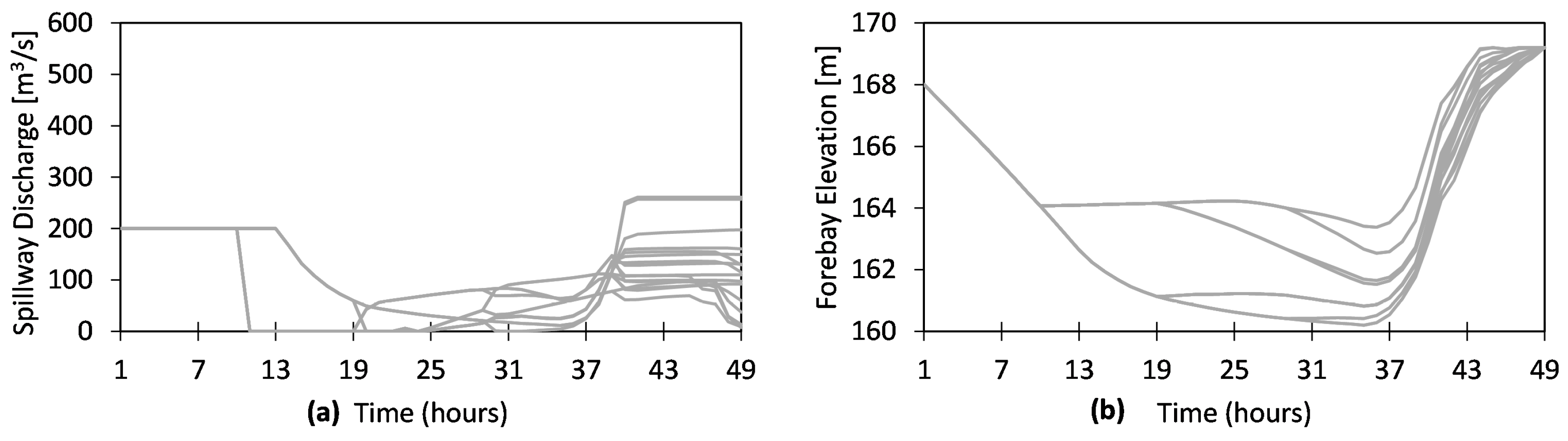
4.2. Deterministic MPC Hindcasts Using DSFs

DSFs are produced as single forecast trajectories by adding random perturbations on observations, thus they under/over-estimate the actual flood inflows. This situation becomes more significant for the refilling season in spring when the initial reservoir forebay elevation is at a critical level. DSF data based MPC hindcasting experiment results using Sce-Q100a data are presented in Figure 8. Likewise, longer forecast horizons than 18 h e.g., 24, 36, and 48 h result in a similar response, thus the experiment results of DSF24, DSF36, and DSF overlap in the figure. According to the results, spillway discharges are greater than the upper limit of 200 m3/s and create flooding in the downstream. This is considered as lower reliability compared to perfect data based experiments, and mainly attributed to the forecast disturbance which introduces 30% bias to the control strategy. Longer forecast horizons (such as 18, 24, 36, 48 h) perform better and releases are shifted to earlier time steps. However, it is not possible to mitigate the flood event even for forecast horizons longer than 18 h due to the given bias in the inflows and the lack of uncertainty in the system optimization. Compared to perfect forecasts based MPC, the variations in spillages are higher due to updated information for each receding horizon.

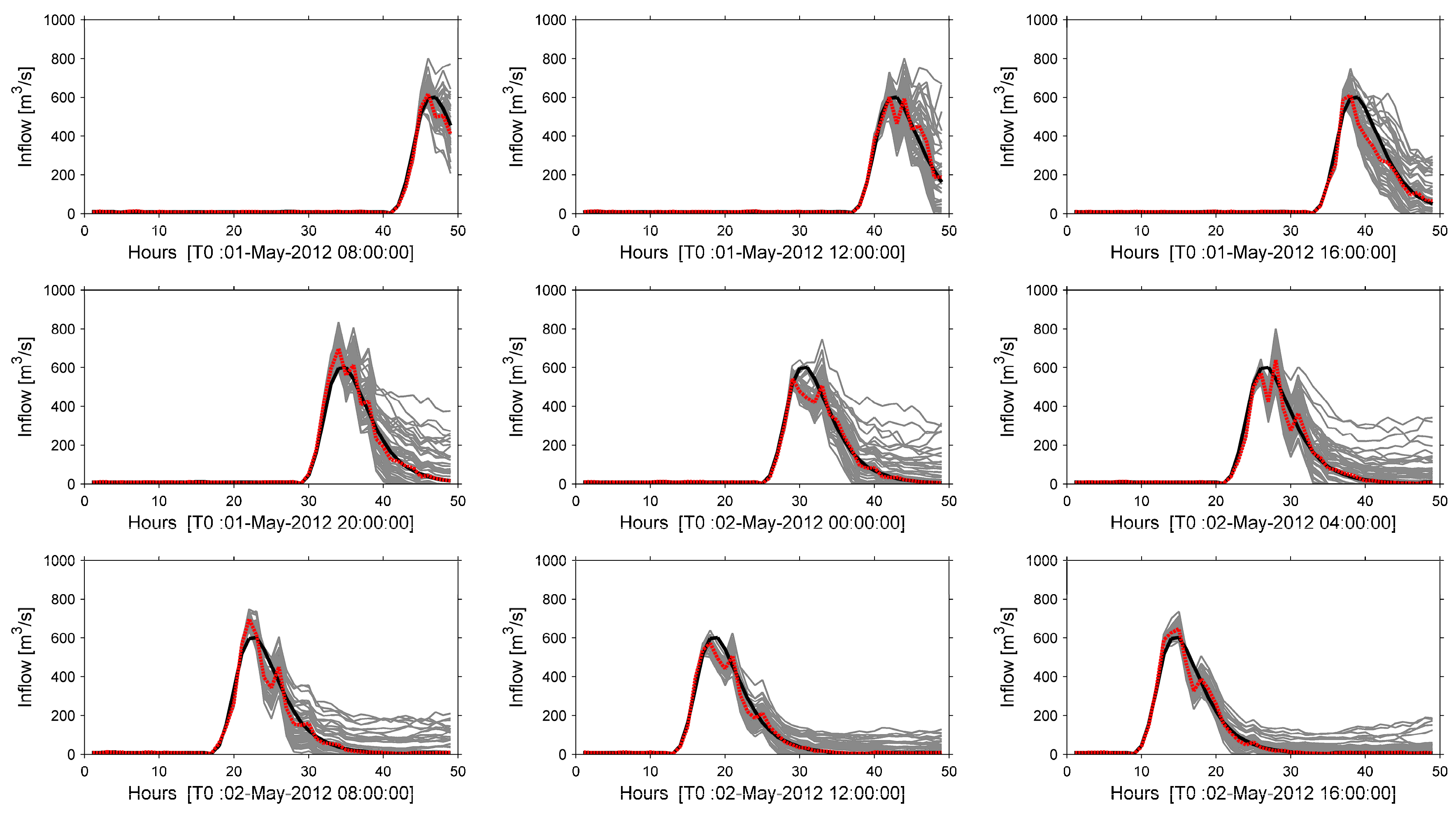
4.3. Multi-Stage Stochastic TB-MPC Hindcasts Using PSFs

In this part, hindcasting experiments are conducted by means of PSF data and multi-stage stochastic optimization. TB-MPC uses scenario trees for disturbances (inflows), states (forebay elevation) and control trajectories (spillway discharges) to form a related stochastic model. Definition of the multiple stages at branching points using binary trees makes the process a multi-stage stochastic optimization in TB-MPC. Hence, the results become more adaptive to the resolution of uncertainty and have better expected performances.
MPC solves an open-loop optimization at every time instant along a forecast horizon and applies only to the first control value to the system. Therefore, an example from a selected single case [T0 = 2-May-2012 14:00:00] of open-loop optimization results is presented with spillway discharge and forebay elevation in smooth trees (Figure 9). One can note that the use of binary trees splits the stochastic variables into two trajectories at each specific branching point. The timing of specific branching points is automatically defined due to the tree-reduction algorithm (check Section 2.3) when the branch number and optimization forecast horizon have been fixed. In this study, 16 tree branches were chosen based on the performance comparison (check Section 4.3.1) for the forecast horizon of 48 h (check Section 4.3.2), thus branching points are fixed every 10 h by the tree reduction algorithm. The root value is an optimal discharge for the entire control sequence considering uncertainty resolution through the forecast horizon. Only single discharge data from a rooted tree of the open-loop optimization is used in the simulation, and the process is shifted to the next time step. At the following time instant, the optimization is reformulated with the updated initial reservoir level and updated forecast data. After applying this procedure through the whole hindcast period (96 h), closed-loop TB-MPC hindcasting experiment results (one single output) are obtained. These results are discussed under the subsections of Section 4.3.

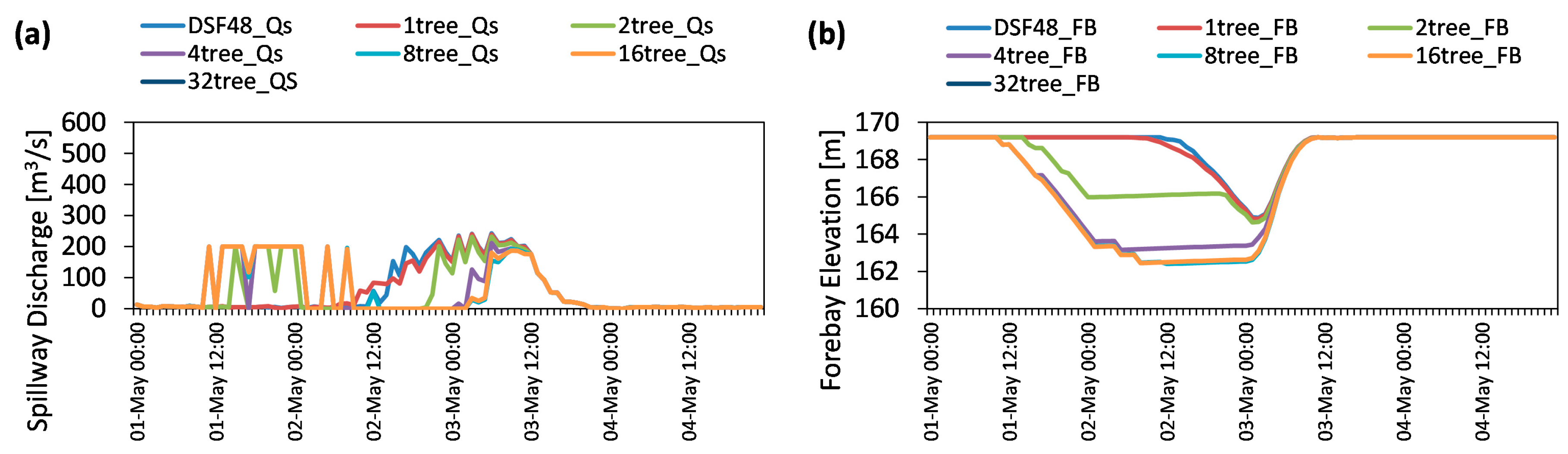
4.3.1. TB-MPC Hindcasts Considering a Different Number of Tree Branches

The number of tree branches used in TB-MPC is user-defined and there is no direct method to select the most appropriate one. In this part, performances of TB-MPC hindcasting experiments using Sce-Q100a data are conducted by selecting a different number of tree branches in each trial and the results are compared with each other. According to TB-MPC methodology, total PSF members can be reduced to 2x branches, e.g., 1, 2, 4, 8,… etc. [24]. Therefore, in this study 50 PSF ensembles were reduced to six different branches (1, 2, 4, 8, 16 and 32) and tested in a hindcast test. The experiments were done using Sce-Q100a PSF as input forecast data and comparison of the optimization results from different tree branches numbers is given in Figure 10 in terms of spillway flows and forebay elevation. This experiment shows the effects of the resolution of tree and correspondingly capturing forecast uncertainty in stochastic optimization. If the forecast horizon is set to 48 h, we can get optimum results after 16 branches as shown (Figure 10a) in terms of the spillway discharge. Since the results for 16–32 trees are exactly the same, they overlap with each other in the same figure. Although higher resolution overestimates the inflows which increases the pre-releases, it is still able to restore the forebay elevation target at the end of the flood event (Figure 10b).
The computation time is given for different tree reduction branches in the hindcasting experiments in comparison with deterministic MPC with DSF (Table 2). Note that this is the total time for the entire hindcast period (96 h). The time spent in deterministic MPC is three times less than TB-MPC with one tree branch which can be considered as the ensemble mean. This is mainly attributed to the tree reduction process before the optimization of the model. However, the computation time increases as long as higher tree branches are used in the model. Therefore, the tree number is fixed to 16 branches for the following experiments of the study. These results are also valid for the remaining scenarios.

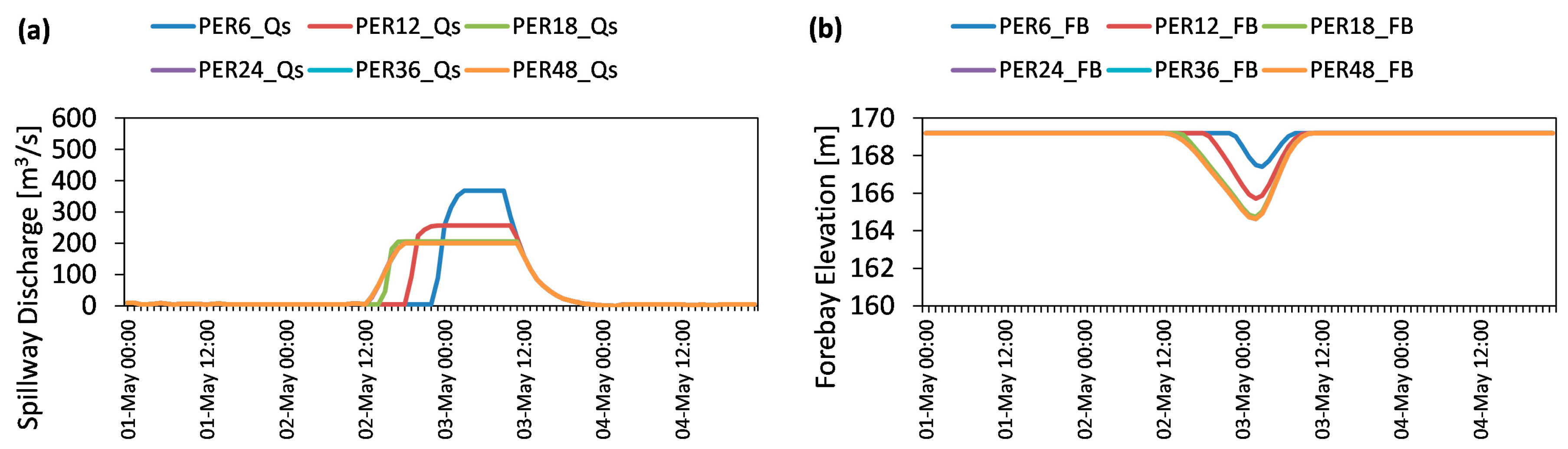
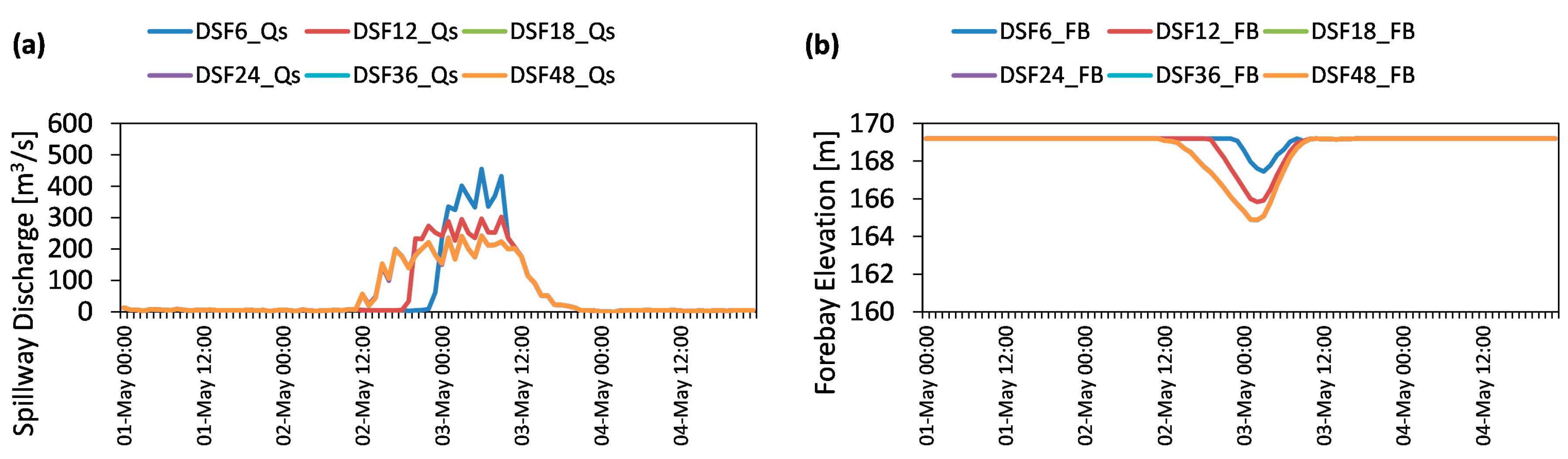
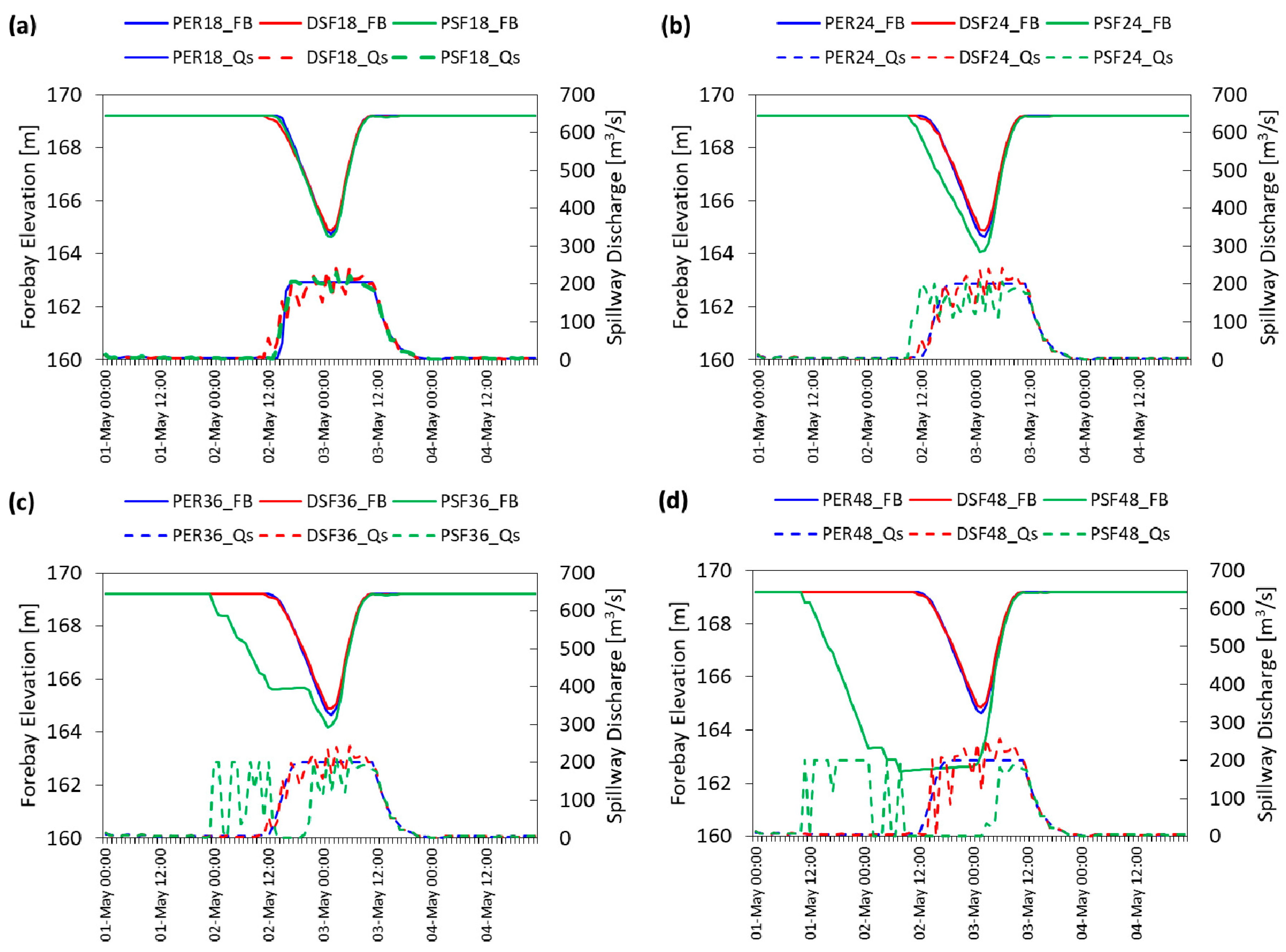
4.3.2. TB-MPC Hindcasts Considering Different Forecast Horizons

Figure 11 presents a comparative visualization of different hindcasting experiments with perfect data and DSF under deterministic configuration and PSF under multi-stage stochastic TB-MPC for 18, 24, 36, and 48 h forecast horizons. Notice that deterministic methods have similar results for a longer forecast horizon whereas TB-MPC start earlier pre-releases. This is mainly attributed to consideration of uncertainty resolution through the forecast horizon in the decision mechanism. When the selected forecast horizon increases in TB-MPC experiments, the uncertainty band in the PSF spread increases and thereby much more water is evacuated from the spillway with the more conservative policy for flood control. It is remarkable to note that even when a longer forecast horizon is selected, forebay elevations at the end of the flood event are always equal to the initial reservoir elevation. These results are also valid for the remaining scenarios.

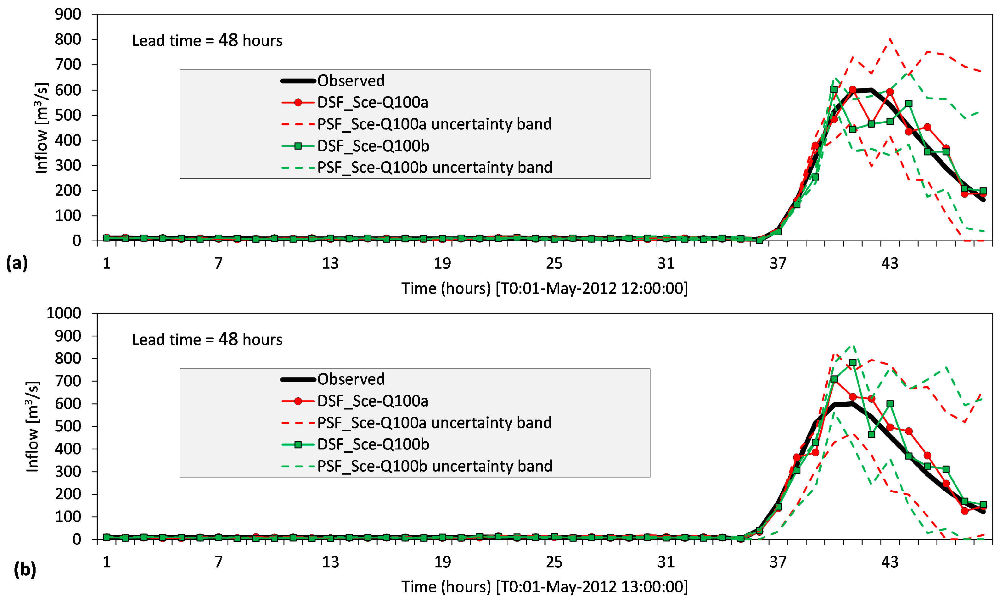
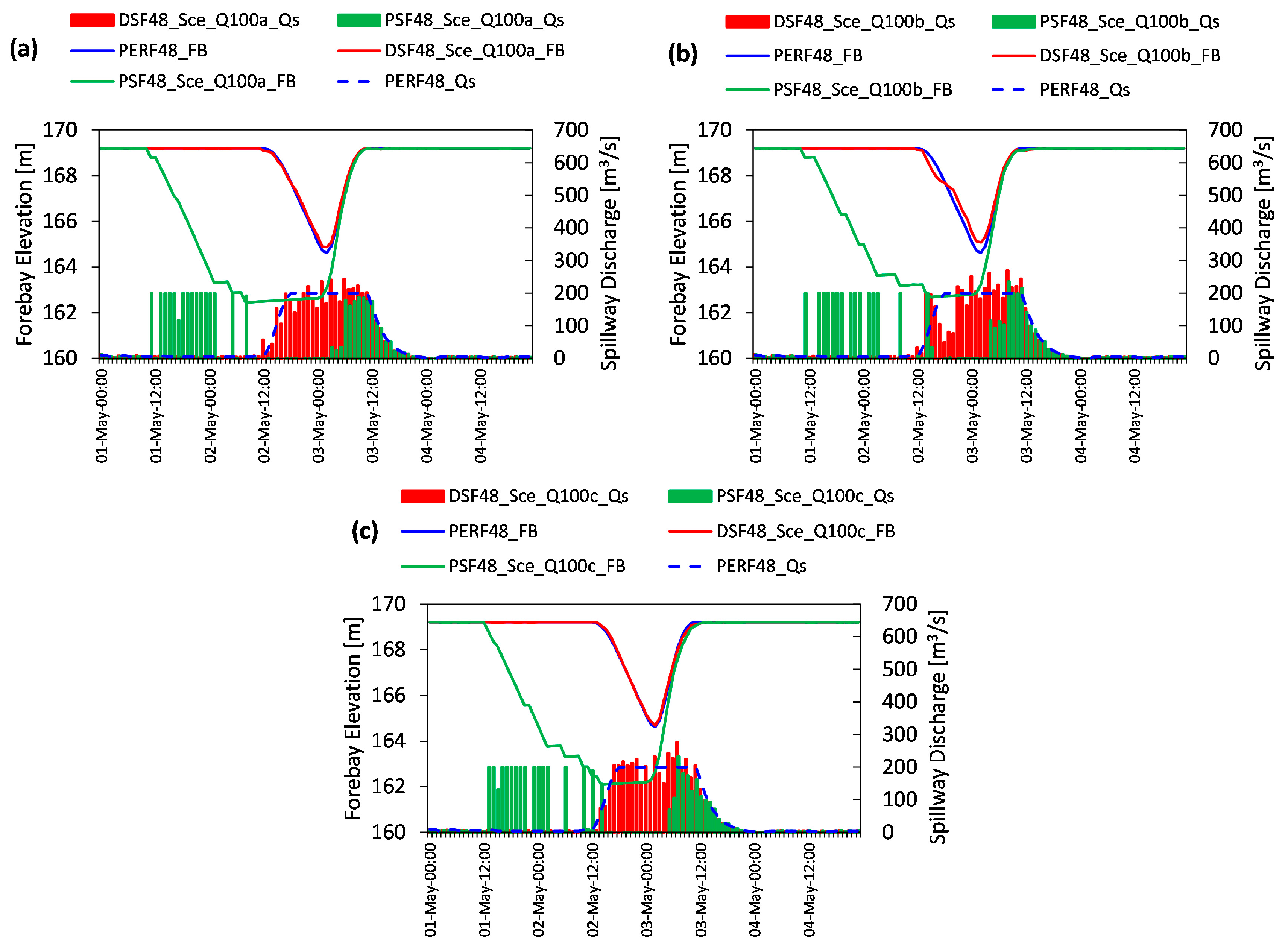
4.3.3. Assessment of the Approach for Different Inflow Conditions and Scenarios

The hindcasting experiments having forecast horizons of 48 h were enriched with different inflow conditions to check the robustness of the developed methodology. To that end, hydrographs characterized by return periods lower than 100 years such as 25 and 50 years, which have peak flows greater than the downstream channel capacity, were also used in the closed-loop hindcasting experiments. All experiments were evaluated by forebay elevation at the end of the flood event, the penalization of the flooding threshold value by the peak flow observed at the Yuvacık outlet, the total flood volume at the downstream area, and FSI. Similar to the previous set-up, flood hydrographs were independently utilized in each hindcasting test as perfect data, DSF and PSF data sets were generated. The tests were also elaborately investigated with three different independent scenarios (a,b,c) for each flow condition. The complete results belonging to the hindcasting experiments are given in Supplementary Figures S2 and S3 for Q25 and Q50 scenarios, respectively. On the other hand, deterministic (perfect and DSF) and stochastic (PSF) closed-loop MPC results from Sce-Q100a, Sce-Q100b and Sce-Q100c are shown in Figure 12. It is notable that the stochastic set-up always provides pre-releases and takes precautions against flood event. The deterministic model only takes actions over several hours which is similar to the perfect data based reference model, but generates much more spillage above the flood threshold compared to stochastic TM-MPC.
A brief summary of all inflow conditions for the three scenarios are given (Table 3) in terms of peak flow values. Since perfect data based models can give the desired maximum spillway of 200 m3/s for each condition, they are not shown in the table. According to results, there is always an improvement in spillway discharges for different flows conditions of Q25, Q50 and Q100.
Table 4 presents the total flood volumes at the downstream area calculated in the hindcasting period. Compared to flooding threshold assessment, this indicator provides more insight into spillway operation. The best management (zero volume) is possible by perfect data using a forecast horizon of 48 h. Almost in all inflow cases and scenarios, the total flood volume decreases in the stochastic mode. This change highlights the added value of the stochastic optimization in comparison to the deterministic one especially for different forecast data sets (scenarios) and different flow conditions. FSI values were also calculated for both DSF and PSF scenarios and results are presented in Table 5, respectively. It is important to note that each FSI is calculated according to its own FCL i.e., FCL Q100 is used for Q100 operation assessment whereas FCL Q50 is used for the Q50 based flood case. According to this, TB-MPC stands as the more confident by higher FSI but also still can provide a high reservoir level at the end of the event without compromising water supply targets. For an uncertain future, a higher FSI is more reliable and preferable with lower risk for water supply as well.
According to results, PSF based multi-stage stochastic MPC optimization has the advantage of including forecast uncertainty in the optimization set-up. Also, the uncertainty in the flows can be represented in the synthesized PSFs by developing the proposed error generation method. There is always performance improvement in the TB-MPC model for flood flows of Q25, Q50, Q100 with a forecast horizon up to 48 h with respect to (i) maximum discharge at the dam outlet (compared to flooding threshold value), (ii) total flood volume at the downstream area and (iii) FSI, while keeping the forebay elevation at the desired level for water supply at the end of the flood event. This shows the added value of the approach and provides reasonable outputs compared to the deterministic counterpart. The developed framework also indicates robust solutions against forecast uncertainty along with a different independent hindcasting experiment assessment.

5. Conclusions and Outlook

This study shows the added value of stochastic optimization using a synthetic probabilistic forecast generation and mass-conservative scenario tree reduction technique. TB-MPC provides multi-stage stochastic optimization in comparison to its deterministic counterpart. According to hindcasting experiments, our main conclusions are:
  • Forecast uncertainty is indispensable especially for flood management. It is critical for those cases in which wrong or poor decisions may result with loss of life and property. At this point, considering uncertainty provides better management in terms of flood metrics without discarding water supply purposes.
  • Independent closed-loop hindcasting experiment scenarios demonstrate the robustness of the system developed against biased information (disturbances).
  • Probabilistic data represent forecast uncertainty in comparison to deterministic equivalents. In this study, a new synthetic streamflow generation method is proposed to represent forecast uncertainty for reservoir optimization.
  • The synthetic PSF generation model that considers the dynamic evolution of uncertainties is valuable if hydrological model outputs driven by a rainfall and temperature forecast ensemble are not available. This method is very advantageous from the operational standpoint, since it does not require complex computations and is easy to implement while considering conditional (flow dependent) increasing uncertainty through time. It is simple to formulate, comprehend, and easy to repeat.
  • Besides the ensemble generation, tree reduction parameters should be carefully investigated in the problem definition phase. In the case of selecting a lower branch and forecast horizon than required, TB-MPC results may converge to deterministic MPC results.
  • The system was also tested against different inflow conditions which have greater flood value than the downstream channel capacity. According to the results, the method provides reliable results against different high flood conditions in the hindcasting experiments.
In future work, a hydrological model will be used, thus synthesized PSF might be derived from perturbed hydrological model forcings such as precipitation and temperature. A comparison of these results can contribute to improve synthetic ensemble generation and its consideration in TB-MPC.

Supplementary Materials

The following are available online at https://www.mdpi.com/2073-4441/10/3/340/s1, Figure S1: mean CRPS of ensemble scenarios: (a) Sce-Q25; (b) Sce-Q50; (c) Sce-Q100, Figure S2: Comparison of deterministic (perfect and DSF) and stochastic (PSF) closed-loop MPC results with different forecast scenarios for Q25: (a) Sce-Q25a; (b) Sce-Q25b; (c) Sce-Q25c, Figure S3: Comparison of deterministic (perfect and DSF) and stochastic (PSF) closed-loop MPC results with different forecast scenarios for Q50: (a) Sce-Q50a; (b) Sce-Q50b; (c) Sce-Q50c.

Acknowledgments

The first author would like to thank The Scientific and Technological Research Council of Turkey (TUBITAK) for the scholarship (2214A program). This study is supported by Anadolu University Scientific Research Projects Commission (under the grant No: 1506F502 and No: 1705F189). Graphs were prepared by Daniel’s XL Toolbox (www.xltoolbox.net) and MATLAB 2012a (License number: 991708).

Author Contributions

Aynur Şensoy set the problem and background. Gökcen Uysal organized the main structure of the paper. Gökcen Uysal, Rodolfo Alvarado-Montero, and Dirk Schwanenberg designed the methodology. Gökcen Uysal conducted the experiments, and prepared the draft paper. Finally, Dirk Schwanenberg, Rodolfo Alvarado-Montero, and Aynur Şensoy provided useful advice and made some corrections. All authors read and approved the final manuscript.

Conflicts of Interest

The authors declare no conflict of interest.

References

  1. Ahmad, S.; Simonovic, S.P. System dynamics modeling of reservoir operations for flood management. J. Comput. Civ. Eng. 2000, 14, 190–198. [Google Scholar] [CrossRef]
  2. Plate, E.J. Flood risk and flood management. J. Hydrol. 2002, 267, 2–11. [Google Scholar] [CrossRef]
  3. Wei, C.C.; Hsu, N.S. Optimal tree-based release rules for real-time flood control operations on a multipurpose multireservoir system. J. Hydrol. 2009, 365, 213–224. [Google Scholar] [CrossRef]
  4. Şensoy, A.; Uysal, G.; Şorman, A.A. Developing a decision support framework for real-time flood management using integrated models. J. Flood Risk Manag. 2016. [Google Scholar] [CrossRef]
  5. Cheng, W.M.; Huang, C.L.; Hsu, N.S.; Wei, C.C. Risk analysis of reservoir operations considering short-term flood control and long-term water supply: A case study for the Da-Han Creek Basin in Taiwan. Water 2017, 9, 424. [Google Scholar] [CrossRef]
  6. Oliveira, R.; Loucks, D.P. Operating rules for multireservoir systems. Water Resour. Res. 1997, 33, 839–852. [Google Scholar] [CrossRef]
  7. Chang, F.J.; Chen, L.; Chang, L.C. Optimizing the reservoir operating rule curves by genetic algorithms. Hydrol. Process. 2005, 19, 2277–2289. [Google Scholar] [CrossRef]
  8. Liu, P.; Guo, S.; Xu, X.; Chen, J. Derivation of aggregation-based joint operating rule curves for cascade hydropower reservoirs. Water Resour. Manag. 2011, 25, 3177–3200. [Google Scholar] [CrossRef]
  9. Rani, D.; Moreira, M.M. Simulation–optimization modeling: A survey and potential application in reservoir systems operation. Water Resour. Manag. 2010, 24, 1107–1138. [Google Scholar] [CrossRef]
  10. Li, X.; Guo, S.; Liu, P.; Chen, G. Dynamic control of flood limited water level for reservoir operation by considering inflow uncertainty. J. Hydrol. 2010, 391, 124–132. [Google Scholar] [CrossRef]
  11. Wan, W.; Zhao, J.; Lund, J.R.; Zhao, T.; Lei, X.; Wang, H. Optimal hedging rule for reservoir refill. J. Water Resour. Plan. Manag. ASCE 2016, 142, 04016051. [Google Scholar] [CrossRef]
  12. Bellman, R. The theory of dynamic programming. Bull. Am. Math. Soc. 1954, 60, 503–516. [Google Scholar] [CrossRef]
  13. Faber, B.A.; Stedinger, J.R. Reservoir optimization using sampling SDP with ensemble streamflow prediction (ESP) forecasts. J. Hydrol. 2001, 249, 113–133. [Google Scholar] [CrossRef]
  14. Yurtal, R.; Seckin, G.; Ardiclioglu, G. Hydropower optimization for the lower Seyhan system in Turkey using dynamic programming. Water Int. 2005, 30, 522–529. [Google Scholar] [CrossRef]
  15. Raso, L.; Malaterre, P.O.; Bader, J.C. Effective streamflow process modeling for optimal reservoir operation using stochastic dual dynamic programming. J. Water Resour. Plann. Manage. ASCE 2017, 143, 04017003. [Google Scholar] [CrossRef]
  16. Labadie, J.W. Optimal operation of multireservoir systems: State-of-the-art review. J. Water Resour. Plan. Manag. ASCE 2004, 130, 93–111. [Google Scholar] [CrossRef]
  17. Morari, M.; Lee, J.H. Model predictive control: Past, present and future. Comput. Chem. Eng. 1999, 23, 667–682. [Google Scholar] [CrossRef]
  18. Blanco, T.B.; Willems, P.; Chiang, P.K.; Haverbeke, N.; Berlamont, J.; De Moor, B. Flood regulation using nonlinear model predictive control. Control Eng. Pract. 2010, 18, 1147–1157. [Google Scholar] [CrossRef]
  19. Van Overloop, P.J.; Horváth, K.; Aydin, B.E. Model predictive control based on an integrator resonance model applied to an open water channel. Control Eng. Pract. 2014, 27, 54–60. [Google Scholar] [CrossRef]
  20. Horváth, K.; Galvis, E.; Valentín, M.G.; Rodellar, J. New offset-free method for model predictive control of open channels. Control Eng. Pract. 2015, 41, 13–25. [Google Scholar] [CrossRef]
  21. Zhao, T.; Zhao, J.; Yang, D.; Wang, H. Generalized martingale model of the uncertainty evolution of streamflow forecasts. Adv. Water Resour. 2013, 57, 41–51. [Google Scholar] [CrossRef]
  22. Chen, J.; Brissette, F.P.; Leconte, R. Uncertainty of downscaling method in quantifying the impact of climate change on hydrology. J. Hydrol. 2011, 401, 190–202. [Google Scholar] [CrossRef]
  23. Roulin, E.; Vannitsem, S. Post-processing of medium-range probabilistic hydrological forecasting: Impact of forcing, initial conditions and model errors. Hydrol. Process. 2015, 29, 1434–1449. [Google Scholar] [CrossRef]
  24. Fan, F.M.; Schwanenberg, D.; Alvarado, R.; dos Reis, A.A.; Collischonn, W.; Naumman, S. Performance of deterministic and probabilistic hydrological forecasts for the short-term optimization of a tropical hydropower reservoir. Water Resour. Manag. 2016, 30, 3609–3625. [Google Scholar] [CrossRef]
  25. Kuczera, G.; Parent, E. Monte Carlo assessment of parameter uncertainty in conceptual catchment models: The Metropolis algorithm. J. Hydrol. 1998, 211, 69–85. [Google Scholar] [CrossRef]
  26. Montero, R.A.; Schwanenberg, D.; Krahe, P.; Lisniak, D.; Sensoy, A.; Sorman, A.A.; Akkol, B. Moving horizon estimation for assimilating H-SAF remote sensing data into the HBV hydrological model. Adv. Water Resour. 2016, 92, 248–257. [Google Scholar] [CrossRef]
  27. Yao, H.; Georgakakos, A. Assessment of Folsom Lake response to historical and potential future climate scenarios: 2. Reservoir management. J. Hydrol. 2001, 249, 176–196. [Google Scholar] [CrossRef]
  28. Zhao, T.; Cai, X.; Yang, D. Effect of streamflow forecast uncertainty on real-time reservoir operation. Adv. Water Resour. 2011, 34, 495–504. [Google Scholar] [CrossRef]
  29. Liu, Z.; Guo, Y.; Wang, L.; Wang, Q. Streamflow forecast errors and their impacts on forecast-based reservoir flood control. Water Resour. Manag. 2015, 29, 4557–4572. [Google Scholar] [CrossRef]
  30. Todini, E. Role and treatment of uncertainty in real-time flood forecasting. Hydrol. Process. 2004, 18, 2743–2746. [Google Scholar] [CrossRef]
  31. Koutsoyiannis, D. The Hurst phenomenon and fractional Gaussian noise made easy. Hydrol. Sci. J. 2002, 47, 573–595. [Google Scholar] [CrossRef]
  32. Ahmed, J.A.; Sarma, A.K. Artificial neural network model for synthetic streamflow generation. Water Resour. Manag. 2007, 21, 1015. [Google Scholar] [CrossRef]
  33. Ochoa-Rivera, J.C.; García-Bartual, R.; Andreu, J. Multivariate synthetic streamflow generation using a hybrid model based on artificial neural networks. Hydrol. Earth Syst. Sci. 2002, 6, 641–654. [Google Scholar] [CrossRef]
  34. Raso, L.; Schwanenberg, D.; van de Giesen, N.C.; van Overloop, P.J. Short-term optimal operation of water systems using ensemble forecasts. Adv. Water Resour. 2014, 71, 200–208. [Google Scholar] [CrossRef]
  35. Stive, P.M. Performance Assessment of Tree-Based Model Predictive Control. Master’s Thesis, Delft University of Technology, Delft, The Netherlands, 2011. [Google Scholar]
  36. Ficchi, A.; Raso, L.; Dorchies, D.; Pianosi, F.; Malaterre, P.O.; van Overloop, P.J.; Jay-Allemand, M. Optimal operation of the multireservoir system in the Seine River Basin using deterministic and ensemble forecasts. J. Water Resour. Plan. Manag. 2015, 142. [Google Scholar] [CrossRef]
  37. Schwanenberg, D.; Fan, F.M.; Naumann, S.; Kuwajima, J.I.; Montero, R.A.; dos Reis, A.A. Short-term reservoir optimization for flood mitigation under meteorological and hydrological forecast uncertainty. Water Resour. Manag. 2015, 29, 1635–1651. [Google Scholar] [CrossRef]
  38. Uysal, G.; Şensoy, A.; Şorman, A.A.; Akgün, T.; Gezgin, T. Basin/reservoir system integration for real time reservoir operation. Water Resour. Manag. 2016, 30, 1653–1668. [Google Scholar] [CrossRef]
  39. Uysal, G.; Schwanenberg, D.; Alvarado-Montero, R.; Şensoy, A. Short term optimal operation of water supply reservoir under flood control stress using model predictive control. Water Resour. Manag. 2018, 32, 583–597. [Google Scholar] [CrossRef]
  40. Hui, P. Yellow River Group Project, A Subproject of the China-DC WRE Project; Final Research Report of Cluster 2; Delft University of Technology: Delft, The Netherlands, 2002. [Google Scholar]
  41. Yan, B.; Guo, S.; Chen, L. Estimation of reservoir flood control operation risks with considering inflow forecasting errors. Stoch. Environ. Res. Risk Assess. 2014, 28, 359–368. [Google Scholar] [CrossRef]
  42. Datta, B.; Burges, S.J. Short-term, single, multiple-purpose reservoir operation: Importance of loss functions and forecast errors. Water Resour. Res. 1984, 20, 1167–1176. [Google Scholar] [CrossRef]
  43. Pianosi, F.; Raso, L. Dynamic modeling of predictive uncertainty by regression on absolute errors. Water Resour. Res. 2012, 48. [Google Scholar] [CrossRef]
  44. Biemans, H.; Hutjes, R.W.A.; Kabat, P.; Strengers, B.J.; Gerten, D.; Rost, S. Effects of precipitation uncertainty on discharge calculations for main river basins. J. Hydrometeorol. 2009, 10, 1011–1025. [Google Scholar] [CrossRef]
  45. Schwanenberg, D.; Becker, B.P.J.; Xu, M. The open real-time control (RTC)-Tools software framework for modeling RTC in water resources sytems. J. Hydroinform. 2015, 17, 130–148. [Google Scholar] [CrossRef]
  46. Xu, M.; Schwanenberg, D. Comparison of sequential and simultaneous model predictive control of reservoir systems. In Proceedings of the 10th International Conference on Hydroinformatics, Hamburg, Germany, 14–18 July 2012. [Google Scholar]
  47. Wächter, A.; Biegler, L.T. On the implementation of an interior-point filter line-search algorithm for large-scale nonlinear programming. Math. Program. 2006, 106, 25–57. [Google Scholar] [CrossRef]
  48. Heitsch, H.; Römisch, W. Scenario reduction algorithms in stochastic programming. Comput. Optim. Appl. 2003, 24, 187–206. [Google Scholar] [CrossRef]
  49. Nadarajah, S.; Shiau, J.T. Analysis of extreme flood events for the Pachang River, Taiwan. Water Resour. Manag. 2005, 19, 363–374. [Google Scholar] [CrossRef]
  50. Stedinger, J.R.; Vogel, R.M.; Foufoula-Georgiou, E. Frequency analysis of extreme events. In Handbook of Hydrology; Maidment, D.R., Ed.; McGraw-Hill: New York, NY, USA, 1993; Chapter 18. [Google Scholar]
  51. Xiao, Y.; Guo, S.; Liu, P.; Yan, B.; Chen, L. Design flood hydrograph based on multicharacteristic synthesis index method. J. Hydrol. Eng. 2009, 14, 1359–1364. [Google Scholar] [CrossRef]
  52. General Directorate of State Hydraulic Works (DSI). Kirazdere Dam Engineering Hydrology and Planning Report; Prepared by 1st Regional Directorate of State Hydraulics Works; Planning and Science Board: Bursa, Turkey, 1983. (In Turkish)
  53. Mediero, L.; Garrote, L.; Martin-Carrasco, F. A probabilistic model to support reservoir operation decisions during flash floods. Hydrol. Sci. J. ASCE 2007, 52, 523–537. [Google Scholar] [CrossRef]
  54. Jørgensen, J.B. Moving Horizon Estimation and Control. Ph.D. Thesis, Technical University of Denmark, Lyngby, Denmark, 2005. [Google Scholar]
Figure 1. The general framework of the experiments. DSFs stands for Deterministic Streamflow Forecasts. PSFs stands for Probabilistic Streamflow Forecasts. MPC stands for Model Predictive Control.
Water 10 00340 g001
Figure 2. Schematic of single time-step streamflow forecast uncertainty: (a) DSF schematization; (b) PSF schematization. q k stands for observed inflow. ε stands for relative inflow forecasting error. q ^ k stands for DSF member. q ˜ j k stands for j t h PSF member. k stands for time index.
Water 10 00340 g002
Figure 3. Yuvacık Basin DEM, station network and downstream region.
Water 10 00340 g003
Figure 4. Graphical representation of the scenarios (Sce-Q100a and Sce-Q100b) for: (a) T0: 01-May-2012 12:00:00; (b) T0: 01-May-2012 13:00:00.
Water 10 00340 g004
Figure 5. Perfect forecast, DSF vs. PSF for different receding horizons (Sce-Q100a).
Water 10 00340 g005
Figure 6. PSF ensemble members (50 members) transformed into optimization trees (16 branches).
Water 10 00340 g006
Figure 7. Comparison of closed-loop MPC forecast horizon performance using perfect streamflow forecasts: (a) Spillway discharge (m3/s); (b) forebay elevation (m).
Water 10 00340 g007
Figure 8. Comparison of closed-loop MPC forecast horizon performances with DSF (Sce-Q100a): (a) Spillway discharge (m3/s); (b) forebay elevation (m).
Water 10 00340 g008
Figure 9. Open-loop optimization results of multi-stage stochastic optimization (from Sce-Q100a): (a) Spillway discharge trees (m3/s); (b) Forebay elevation trees (m).
Water 10 00340 g009
Figure 10. Comparison of closed-loop MPC with different tree reduction branches for 48 h forecast horizon (Sce-Q100a): (a) Spillway discharge (m3/s); (b) forebay elevation (m).
Water 10 00340 g010
Figure 11. Comparison of deterministic (perfect and DSF) and stochastic (PSF) closed-loop MPC results with different forecast horizons (Sce-Q100a): (a) 18 h; (b) 24 h; (c) 36 h; (d) 48 h.
Water 10 00340 g011
Figure 12. Comparison of deterministic (perfect and DSF) and stochastic (PSF) closed-loop MPC results with different forecast scenarios for Q100: (a) Sce-Q100a; (b) Q100-Sceb; (c) Q100-Scec.
Water 10 00340 g012
Table 1. Flood hydrograph peak values.
Return Periods (Years)Project Value (m3/s)
5208
10297
25410
50506
100597
Table 2. Computation times in MPC hindcasting experiments. MPC stands for Model Predictive Control. DSF stands for Deterministic Streamflow Forecast. TB-MPC stands for Tree-based MPC.
Hindcasting ExperimentTotal CPU Time (s)
MPC with DSF151
TB-MPC with 1 tree branch491
TB-MPC with 2 tree branches551
TB-MPC with 4 tree branches633
TB-MPC with 8 tree branches677
TB-MPC with 16 tree branches867
TB-MPC with 32 tree branches1354
Table 3. Peakflow assessment of deterministic and stochastic closed-loop MPC results for different inflow conditions with forecast horizons of 48 h.
Flood HydrographScenariosPeakflow at Yuvacik Outlet (m3/s)
Deterministic MPCStochastic MPC
Q25Sce-Q25a243231
Sce-Q25b255243
Sce-Q25c248243
Q50Sce-Q50a241211
Sce-Q50b245200
Sce-Q50c246200
Q100Sce-Q100a242200
Sce-Q100b269235
Sce-Q100c278233
Table 4. Flood volume assessment of deterministic and stochastic closed-loop MPC for different inflow conditions with forecast horizon of 48 h.
Flood ConditionScenariosTotal Flood Volume (1 × 10⁶ m3)
Deterministic MPCStochastic MPC
Q25Sce-Q25a0.5070.302
Sce-Q25b0.5490.254
Sce-Q25c0.4380.271
Q50Sce-Q50a0.6660.062
Sce-Q50b0.4710.004
Sce-Q50c0.3310.004
Q100Sce-Q100a0.6900.004
Sce-Q100b1.2560.184
Sce-Q100c1.0180.127
Table 5. FSI value assessment of deterministic and stochastic closed-loop MPC according to Flood Control Levels (FCLs) for different inflow conditions with forecast horizon of 48 h.
Flood ConditionScenariosFlood Storage Index (FSI)
Deterministic MPCStochastic MPC
Q25Sce-Q25a0.6520.800
Sce-Q25b0.6590.990
Sce-Q25c0.6590.796
Q50Sce-Q50a0.5660.723
Sce-Q50b0.5980.770
Sce-Q50c0.6060.758
Q100Sce-Q100a0.4570.650
Sce-Q100b0.4630.645
Sce-Q100c0.4560.645

