Evaluating Water Use for Agricultural Intensification in Southern Amazonia Using the Water Footprint Sustainability Assessment

Abstract

We performed a Water Footprint Sustainability Assessment (WFSA) in the Xingu Basin of Mato Grosso (XBMT), Brazil, with the objectives of (1) tracking blue (as surface water) and green water (as soil moisture regenerated by precipitation) consumption in recent years (2000, 2014); and (2) evaluating agricultural intensification options for future years (2030, 2050) considering the effects of deforestation and climate change on water availability in the basin. The agricultural sector was the largest consumer of water in the basin despite there being almost no irrigation of cropland or pastures. In addition to water use by crops and pasture grass, water consumption attributed to cattle production included evaporation from roughly 9463 ha of small farm reservoirs used to provide drinking water for cattle in 2014. The WFSA showed that while blue and green water consumptive uses were within sustainable limits in 2014, deforestation, cattle confinement, and the use of irrigation to increase cropping frequency could drive water use to unsustainable levels in the future. While land management policies and practices should strive for protection of the remaining natural vegetation, increased agricultural production will require reservoir and irrigation water management to reduce the potential threat of blue water scarcity in the dry season. In addition to providing general guidance for future water allocation decisions in the basin, our study offers an interpretation of blue and green water scarcities with changes in land use and climate in a rapidly evolving agricultural frontier.

1. Introduction

Southern Amazonia, Brazil, has experienced significant development since the 1990s, with agricultural production expanding rapidly through land use change in both the Amazon and Cerrado (or savanna) biomes [1]. Natural vegetation cover has been gradually replaced by pasture and soybean land use systems [2], often through a natural vegetation to pasture to cropland transition [3,4]. This increase in agricultural production has had important socio-economic and environmental implications. Socio-economic indicators suggest a growth in the tertiary sector up- and down-stream of soybean production, with evidence of local investment and financial returns [5]. At the same time, deforestation has been shown to alter local climate and water cycles, thereby pushing the Amazon towards a tipping point [6] that could significantly alter the biome. Changes to above and belowground carbon stocks have implications for global climate change [7], while land use change can affect the water cycle by increasing river discharge [8] and diminishing water vapor supply to the atmosphere with implications for regional precipitation [3,9,10]. Changes to the water cycle, in particular, affect economic activity through hydropower generation and agriculture [11,12,13], but can also affect aquatic and terrestrial ecosystems [14,15].

Agricultural expansion in the region has been followed by infrastructure development such as road networks [6], population growth and land use activities that trigger further deforestation. Between 1991 and 2010, the population of Mato Grosso increased from 2 to 3 million, while the animal population increased from 22 to 82 million, led mainly by cattle [16]. These increases put additional pressures on land use and local demand of natural resources, particularly water. Atmospheric feedbacks could negatively affect agricultural production when considering changes to regional climate and precipitation regimes [12], but could also trigger infrastructure investment in irrigation with additional effects on water withdrawals and feedbacks on water resources [15]. Therefore, feedbacks between agricultural production, land use change, and human and animal population growth need to be investigated in order to evaluate future development scenarios in Southern Amazonia.

This study aims to quantify these changes by carrying out a Water Footprint (WF) Sustainability Assessment (WFSA) [17] in the Xingu Basin of Mato Grosso (XBMT) located in Southern Amazonia, an area that has experienced the land use change dynamics described above. Since 2002, the WF has been increasingly used to quantify direct and indirect water use of production and consumption processes as a means to put these activities into a context of regional and global water resources, as well as potential environmental impacts [18,19,20]. In a WF context, water resources are typically separated into blue water (which represents the surface water and groundwater stocks), green water (which characterizes soil moisture stocks regenerated by precipitation [21]), and grey water (i.e., the amount of water required to dilute chemical or thermal pollution loads to ambient water quality standards [17]). When focusing on water quantity in a WFSA, the blue and green WF are compared to local water availability to derive local water scarcity as a step towards formulating a policy recommendation [17]. Many studies have applied WFSAs to derive blue water scarcity at a global scale (e.g., [22,23]), but only one study to date has attempted to quantify green water scarcity [24]. More studies using the concept of green water scarcity are thus needed to verify the full extent of WF assessments [17,25].

We build upon previous research results on the water cycle of XBMT to carry out a WFSA for the 2000‒2015 period. We also evaluate scenarios for 2030‒2031 and 2050‒2051 with the objectives of formulating responses for water resources management based on past and future land and water use decisions. The combination of land use change, climate change and agricultural production scenarios within a blue and green WFSA is informative to both water resources management, and the WF community seeking to apply this assessment regionally. The XBMT represents a unique basin for such a study, given its geographic location in the so-called “arc-of-deforestation” and the importance in future land use change for agricultural production, but also because of agriculture’s reliance on precipitation in the region. The combination of land use and hydrologic data with information on domestic and industrial water consumption remains mostly unexplored in Southern Amazonia. Therefore, there is an opportunity to use such information in a WFSA to provide a greater context for water resources management and inform decision-making for regional production processes.

Following a description of the XBMT and the details of the required steps for the blue and green WFSA (Section 2), we describe our results of past and future blue and green water availabilities and scarcities (Section 3). Then in Section 4, we discuss our results within the context of regional agricultural development and the effects of land and water management on water scarcity, prior to formulating a policy response for land and water resources in the basin.

2. Materials and Methods

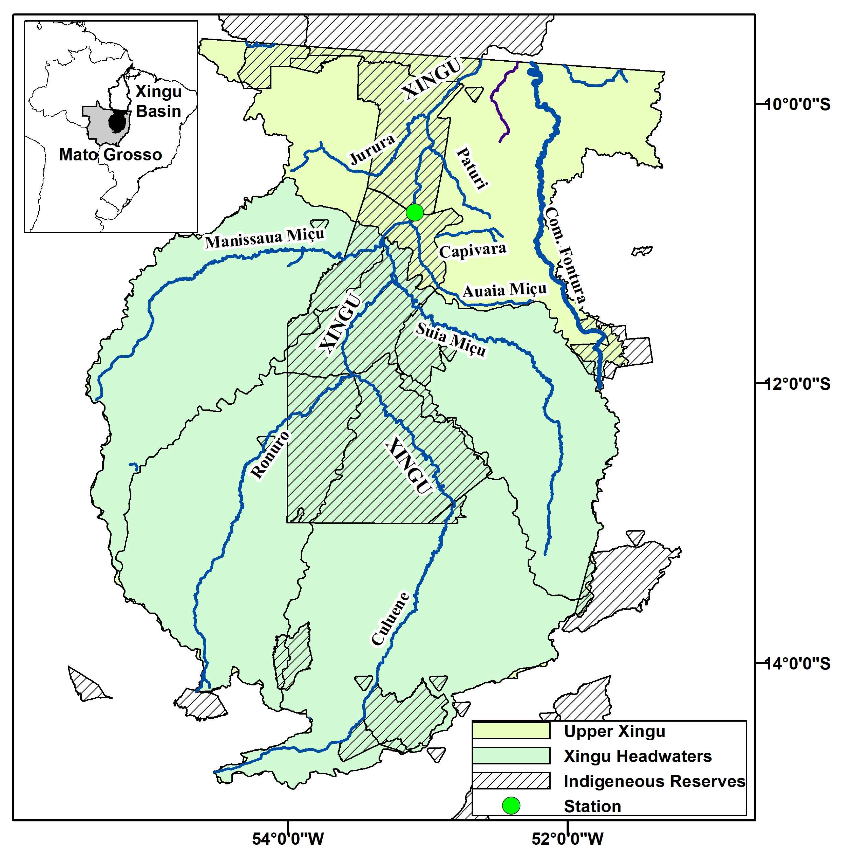
2.1. The Xingu Basin of Mato Grosso

The XBMT (Figure 1) is a 170,000 km² basin located in Southern Amazonia, separated into the Xingu Headwaters (139,000 km²) that flow North into the Upper Xingu Basin (31,000 km²) [26,27], through the state of Pará and into the Amazon River, to constitute the greater Xingu River Basin (510,000 km²) [28]. The XBMT is located at the intersection of both the Amazon (80% of the basin) and Cerrado (20%) biomes and had 50% (85,000 km²) of its forest cover in 2010, of which about 34,000 km² was contained within conservation areas that include parts of the Xingu Indigenous Reserve [9] (Figure 1). Between 2001 and 2010, the XBMT lost 18,838 km² of forest to either cropland (3347 km²) or pasture (15,491 km²) with further evidence of conversion of 4962 km² of pasture into cropland [9]. In 2015, agricultural production for municipalities in the basin consisted of 1.3 Mha of soybean [16], about 5.4 Mha of pasture [10], and less than 12,000 ha of permanent crops (e.g., papayas, bananas, rubber trees) [16]. In addition, the XBMT contains close to 10,000 small farm reservoirs mainly used to supply drinking water for cattle [29]. In 2015, the cattle population reached about 3.5 million heads in the municipalities of the basin [16].

From a total of 199,015 people living in XBMT in 2007, 125,279 made up the urban population (63%), and 73,736 represented the rural population (37%), with the portion serviced by the general water network reaching 47% and 49%, respectively [26]. Most of the drinking water for communities in the Xingu Headwaters is supplied by deep wells (60%), followed by surface water (20%), shallow wells (10%) and a mix of surface water and deep wells (10%), while 100% of the water in the Upper Xingu is supplied exclusively by deep wells [26]. Total domestic water demand was estimated at 0.0208 m³ s⁻¹ in the Xingu Headwaters and 0.1814 m³ s⁻¹ in the Upper Xingu, while industrial demand (as transformation industry) was 0.0023 m³ s⁻¹ and 0.226 m³ s⁻¹, respectively [26]. Given the importance of the agricultural sector in the region, there is additional water demand for livestock, aquaculture with about 47.6 ha of fish tanks, and a total irrigation demand of 1.447 m³ s⁻¹ in 2006 [26].

2.2. Integrated BIosphere Simulator (IBIS)

Hydrology in the XBMT was modeled using the Integrated BIosphere Simulator (IBIS) (v.2.5), which combines ecological processes related to the water and carbon cycles with vegetation dynamics, climate, canopy and vegetation physiology, and phenology on a monthly or annual basis [31,32,33]. IBIS represents the soil-plant-atmosphere continuum to simulate soil moisture and evapotranspiration (ET) through six soil layers to 8 m depth (and soil temperatures), vegetation structure, stomatal conductance and photosynthetic pathways, all forced with atmospheric conditions [31,33]. The model was previously validated by Panday et al. [28] in a study of the water balance of the Xingu River Basin from 2001 to 2010 using atmospheric forcing with data from the Climate Research Unit (CRU TS v.3.2.1). Surface runoff was derived as the difference between ET and the balance of soil moisture, with the latter derived from infiltration (from the Green–Ampt equation) and dynamics in the soil (from the Richards equation) [28].

Following Panday et al. [28], we combine IBIS results with land use maps to derive the monthly water balance of the XBMT for 2000‒2001, 2014‒2015, 2030‒2031, and 2050‒2051 (0.5° resolution, and hydrologic years as September to August) following two simulations: (1) considering the basin’s potential natural vegetation (PNV) as defined by Ramankutty and Foley [34]; (2) considering the replacement of all natural vegetation by C4 grass (G) as a representation of complete deforestation in the basin. Hydrology for 2030‒2031 and 2050‒2051 was obtained from an average of 23 IPCC global climate models and considering two different Representative Concentration Pathways (RCP) of 4.5 and 8.5 W m⁻².

We derived total runoff in the basin through linear association of PNV and G IBIS simulations for the basin in hydrologic year t, defined from September to August of each year [28]

R(t) = R_PNV(t) × F_f(t) + (1 − F_f(t)) × R_G(t)

(1)

where R(t) (mm mo⁻¹) is the monthly discharge in the basin, R_PNV(t) (mm mo⁻¹) is the total runoff in the basin under a PNV simulation, F_f(t) (dimensionless) is the fraction of forest cover in the pixel of interest, and R_G(t) (m³ mo⁻¹) is the total runoff in the G simulation. The fraction F_f(t) was obtained from land cover maps derived from Landsat imagery (30-m resolution) [35], while future land use in 2030 and 2050 was obtained from Soares-Filho et al. [36] based on distinct deforestation scenarios: a business-as-usual scenario (BAU) in which 1997‒2002 deforestation is maintained with planned transportation infrastructure, and a governance scenario (GOV) which assumes similar deforestation rates as BAU, but in which a maximum deforested area representing 50% of each Amazonian sub-region is imposed [36]. When combining climate change with deforestation scenarios, we obtained four distinct scenarios for 2030 and 2050 (BAU_RCP4.5, BAU_RCP8.5, GOV_RCP4.5, GOV_RCP8.5). Values of R(2000), R(2014), R(2030), R(2050) were obtained for the XBMT, and R(2000) was obtained for the Xingu Headwaters and validated against monthly mean river discharge measured at Marcelândia, Mato Grosso (Passagem BR80, station 18430000, 10°46′38″ S, 53°5′44″ W) [30] with a Pearson correlation of 0.83 (see Figure S1 in the Supplemental Material). Values of R(t) were obtained annually and interannually with three-month averages for the years listed above.

Values of R(t) were then used to derive annual basin ET (ET_T(t), mm y⁻¹) using the water balance equation shown in Equation (2), and assuming a change in annual storage close to 0 following findings from Panday et al. [28],

$${\mathrm{ET}}_{\mathrm{T}}\left(\mathrm{t}\right)=\mathrm{P}\left(\mathrm{t}\right)-\mathrm{R}\left(\mathrm{t}\right)$$

(2)

where P(t) (mm y⁻¹) is the precipitation input to the IBIS model. Similarly, we use Equation (2) to derive ET_PNV(t), or the annual ET of the basin under PNV, using R_PNV(t) and the IBIS precipitation input. All values of ET were obtained for 2000, 2014, 2030 and 2050 hydrologic years.

2.3. Water Footprint Sustainability Assessment

2.3.1. Goal and Scope Definition

The goal of this study is to determine changes in blue and green water scarcities from production processes in the XBMT in recent history, and considering deforestation and climate change scenarios for 2030 and 2050, to: (1) provide a hotspot analysis of water use in the basin as guidance for future water allocation decisions; and (2) explore links between blue and green water scarcities in the basin considering land use change histories. This assessment focuses exclusively on water quantity and therefore considers blue and green WFs separately, and does not address water quality as expressed by the grey WF.

2.3.2. Water Footprint Accounting

The accounting step includes the calculation of the blue and green WFs of all processes occurring in the basin for the 2000, 2014, 2030 and 2050 hydrologic years, representing production in recent years (2000, 2014) and defined following distinct scenarios for future conditions (2030, 2050, see Section 2.3.4). The selection of the 2000 and 2014 hydrologic years was based on the intense land use change history in the basin within this time period, as attested by land use maps [9,28,35]. Long-term runoff observation in the Xingu River Basin at Marcelândia [30] showed a change in runoff of −14% (February 2001) and +23% (December 2000) compared to the mean 1975‒2005 discharge. We focus exclusively on production processes, leaving out any local consumption of products that might be produced outside the basin. This assumption is reasonable given the regional focus on agricultural products for export [37], with a majority of crops grown in the region supplied as input feed for livestock. Cropland and pasture in Mato Grosso have been nearly exclusively rainfed [10], and therefore only require green water whose consumption is estimated by ET.

Green Water Footprint of Agriculture in the Context of Basin Land Use Systems

We obtain the green WF of agriculture by combining top-down and bottom-up approaches to track changes in the green WF from 2000 to 2050 hydrologic years (top-down approach) and 2000 to 2014 hydrologic years (bottom-up approach). First, we propose that total annual ET of the XBMT is equal to the sum of contributions from natural vegetation, agricultural land, and a residual term as described in Equation (3)

$${\mathrm{ET}}_{\mathrm{T}}\left(\mathrm{t}\right)={\mathrm{ET}}_{\mathrm{NV}}\left(\mathrm{t}\right)+{\mathrm{ET}}_{\mathrm{AG}}\left(\mathrm{t}\right)+{\mathrm{ET}}_{\mathrm{R}}\left(\mathrm{t}\right)$$

(3)

where ET_T(t) (m³ y⁻¹) is the annual ET in the basin in hydrologic year t obtained from Equation (2), ET_NV(t) (m³ y⁻¹) is the annual ET from natural vegetation (as tropical humid or savanna forest, shrubland, etc.) in the basin, ET_AG(t) (m³ y⁻¹) is the annual ET from agricultural land (as cropland and pasture combined), and ET_R(t) (m³ y⁻¹) is a residual ET term, which accounts for other land use systems (e.g., forest clearance, urban areas, etc.) and water bodies (e.g., rivers, wetlands) that may or may not be included in human consumption activity. In the top-down approach, we extract ET_AG(t) + ET_R(t) from a calculation of ET_NV(t) in Equation (4)

$${\mathrm{ET}}_{\mathrm{NV}}\left(\mathrm{t}\right)={\displaystyle \sum }_{\mathrm{j}}{\mathrm{ET}}_{\mathrm{PNV},\mathrm{j}}\left(\mathrm{t}\right){\mathrm{A}}_{\mathrm{NV},\mathrm{j}}\left(\mathrm{t}\right){\mathrm{F}}_{\mathrm{NV},\mathrm{j}}\left(\mathrm{t}\right)$$

(4)

where ET_NV(t) (m³ y⁻¹) is the natural vegetation ET contribution in the basin, ET_PNV,j(t) (m y⁻¹) is the ET of the IBIS PNV simulation for each IBIS raster j of area A_NV,j(t) (3080 10⁶ m²) within the basin, and considering the fraction of forested land F_NV,j(t) (dimensionless). This approach allowed for the disaggregation of ET_T into ET_NV and (ET_AG + ET_R), which we use to analyze the hydrologic years between 2000 and 2050.

The bottom-up approach was applied for the 2000 and 2014 hydrologic years in which we used average pasture and cropland ET estimates from Lathuillière et al. [10,38] together with land use estimates extracted from Landsat imagery [35]. We considered single- and double-cropped soybean (with rice or maize) as the main crops in the region (Table S1). This assumption is reasonable considering that between 2000 and 2014, soybean represented 48–69% of total annual cropland in the basin, while maize and rice represented 12–23% and 33–3%, respectively [16] with an ever increasing amount of maize double cropping in Mato Grosso [39]. During the same time period, perennial crops represented less than 1% of total agricultural land [16] and were therefore not considered further in this green water accounting step. Residual ET (ET_R) was then derived using Equation (3) and, in this approach, may include ET that could be allocated to a production activity occurring in urban areas, or other landscapes with no immediate productive activity (e.g., ET following forest clearance). Differences in ET_R between the top-down and bottom-up approaches may be interpreted as a systematic error in the allocation of ET to a particular land use systems or human activity.

Blue Water Footprint of Agriculture

The blue WF of agriculture includes irrigation, but also water consumption from livestock production systems. In 2006, about 770 ha of perennial crops were irrigated within XBMT and therefore we assume that the majority of irrigation in the XBMT was not applied to soybean or pasture between 2000 and 2015. Blue water use was estimated for livestock production systems in pasture (ruminants), as well as confined facilities (chicken and swine), and includes drinking water as well as water used for washing of animal housing. Feed for all livestock production was assumed to be sourced from within the region, and is therefore already accounted for in the agricultural green WF (see above). Water consumption for cattle follows the steps described in Lathuillière et al. [40], who allocated green and blue water per kg of live weight based on sex, animal development stage and diet. Here, we consider drinking water sourced from small farm reservoirs in the basin detected by remote sensing [40]. All other animals were assumed to have their drinking water sourced by the main water system. As described in Lathuillière et al. [40], cattle population reported by agricultural production data [16] is a total animal population which does not consider the annual live population in their different stages of development. The annual live animal population for municipality i and calendar year t is the difference between the total herd population (H_i,t) and the number of animals slaughtered (0.17H_i,t). The live annual population L_i,t can then be expressed by

$${\mathrm{L}}_{\mathrm{i},\mathrm{t}}=0.27{\mathrm{H}}_{\mathrm{i},\mathrm{t}}+\left({\mathrm{L}}_{\mathrm{i},\mathrm{t}}-0.27{\mathrm{H}}_{\mathrm{i},\mathrm{t}}-0.17{\mathrm{H}}_{\mathrm{i},\mathrm{t}+1}\right)+0.17{\mathrm{H}}_{\mathrm{i},\mathrm{t}+1}$$

(5)

where 0.27H_i,t is the sum of the calf population (15–18 month duration), L_i,t − 0.27H_i,t − 0.17H_i,t+1 is the sum of the adult population (24–27 month duration), and 0.17H_i,t+1 is the animal population in the finishing stages (to be slaughtered in calendar year t + 1, 6–8 month duration) [40]. Sheep and goat annual offtake rates were assumed identical to that of cattle (17%), while horses, donkeys, and mules were not considered to be consumed and therefore their live population was equated to the total herd population reported by the Brazilian Institute of Geography and Statistics (IBGE as the Portuguese acronym) [16].

The swine and chicken development cycles were assumed to be 70 and 42 days respectively [41,42], from which we derived average swine and chicken populations following Equation (6) [43]

$$\overline{{\mathrm{P}}_{\mathrm{k},\mathrm{i}}\left(\mathrm{t}\right)}=days\frac{{\mathrm{P}}_{\mathrm{k},\mathrm{i}}\left(\mathrm{t}\right)}{365}$$

(6)

where $\overline{{\mathrm{P}}_{\mathrm{k},\mathrm{i}}\left(\mathrm{t}\right)}$. (animals) is the average population of animal k, in municipality i and calendar year t, days is the total number of days of the animal’s development cycle, and P_k,i(t) is the population of animal k reported by national statistics [16]. To reflect animal population information available from IBGE [16] for calendar years into the hydrologic years used in this study, we take the average of the two consecutive calendar years that overlap with each hydrologic year. Similar to crops, animal population for each municipality located inside the basin was scaled based on the percent area located inside XBMT (Table S2).

vestock water consumption was derived following the National Water Agency (ANA as the Portuguese acronym) [26] and Food and Agriculture Organization (FAO) [44] which provide water demand per animal, assuming an average adult consumption. For confined swine and chicken production we assumed 0.0034 m³ animal⁻¹ used to clean animal housing after slaughter following Palhares [42] for swine, which was also assumed for chicken housing. These volumes are assumed to be entirely consumed. While our drinking water consumption estimate is based on adult animal water demand and likely constitutes an overestimation of animal blue water consumption, our water consumption estimate for cleaning is likely an underestimate given the housing turnaround for both swine (70 days) and chicken (42 days) production (Table S2). Large and small ruminants were not allocated any water for cleaning as they were assumed to spend their lifetime in pasture.

Domestic and Industrial Blue Water Footprints

We estimated domestic water consumption based on urban and rural human populations within the basin and the total population receiving municipal services based on information from ANA [26]. We assumed a constant population growth in the basin at a rate of 3.0% y⁻¹ until 2014–2015 [16]. By assuming a total basin population of 199,015 in 2010 (the same as the 2007 information reported by ANA [26]), we derived total population in the remaining years, maintaining the same proportion of urban and rural population not serviced by the municipal system (47% and 49%, respectively) (Table S3). Water consumption was calculated assuming a 50% return flow to surface water, and based on a rural water demand of 70 10⁻³ m³ d⁻¹ cap⁻¹ and an urban demand of 0.260 m³ d⁻¹ cap⁻¹. The 47% of the urban population that was not serviced by the municipalities was assigned a water demand equal to rural demand [26] (Table S3).

Industrial water consumption was based on the number of industrial workers in both extraction and transformation industries assuming an industrial demand of 3.5 m³ d⁻¹ cap⁻¹ [26]. In 2010, the number of industrial workers was 4.1% of the total population within the basin [16], which we assumed to be of constant proportion between 2000 and 2015. Similar to domestic water consumption, we assumed a 50% return flow of industrial water (Table S3).

2.3.3. Water Scarcity Calculation

We estimate water scarcity within the XBMT in hydrologic year t following Equation (7) [17]

$$\mathrm{WS}\left(\mathrm{t}\right)=\frac{{{\displaystyle \sum }}_{\mathrm{j}}{\mathrm{WF}}_{\mathrm{j}}\left(\mathrm{t}\right)}{\mathrm{WA}\left(\mathrm{t}\right)}$$

(7)

where WS(t) (dimensionless) is the water scarcity, WF_j(t) (m³ y⁻¹) is the WF of all activities j (determined in Section 2.3.2), and WA(t) (m³ y⁻¹) is the water available in the basin over time t. Values of WS(t) are defined for both blue and green water and vary from 0 (no scarcity) to 1 (extreme scarcity) to gauge how water use has evolved within the basin. For both blue and green water resources, WA(t) is defined following Equations (8) and (9) [17]

$${\mathrm{WA}}_{\mathrm{B}}\left(\mathrm{t}\right)=\mathrm{R}\left(\mathrm{t}\right)-\mathrm{EFR}$$

(8)

$${\mathrm{WA}}_{\mathrm{G}}\left(\mathrm{t}\right)={\mathrm{ET}}_{\mathrm{T}}\left(\mathrm{t}\right)-{\mathrm{ET}}_{\mathrm{RNV}}\left(\mathrm{t}\right)-{\mathrm{ET}}_{\mathrm{UN}}\left(\mathrm{t}\right)$$

(9)

where WA_B(t) (m³ y⁻¹) is the blue water availability, R(t) (m³ y⁻¹) is the natural discharge (or discharge without human appropriation in the basin, defined in Equation (1)), and EFR (m³ y⁻¹) is the environmental flow requirement defined for the XBMT. When considering our top-down WF accounting approach, the value of EFR was defined according to mean annual runoff following Smakhtin et al. [45] with a value of 45.9 km³ y⁻¹ to keep natural ecosystems in a “fair” condition (see Supplemental Material). When considering our bottom-up WF accounting approach, values of EFR were defined for each 3-month mean discharge between 2000 and 2014 hydrologic years as 0.20R(t) following Richter et al. [46]. Green water availability in hydrologic year t, WA_G(t) (m³ y⁻¹), was obtained by subtracting from the ET_T(t) (m³ y⁻¹) the ET reserved to natural vegetation, as ET_RNV(t) (m³ y⁻¹), and the ET of areas agriculturally unproductive, ET_UN(t) (m³ y⁻¹). We interpret ET_UN(t) as the amount of small reservoir evaporation for cattle production whose area we consider unavailable for agricultural expansion. The value of ET_RNV(t) is interpreted as a percentage of total basin ET (ET_T(t)) as measured in the 2000 hydrologic year and based on the Federal Forest Code minimum requirements for natural forest cover in both the Amazon (80%), Cerrado (35%), and transition (50%) zones [47]. As a result, WA_G and WS_G were calculated using these three minimum requirements expressed in ET_RNV(t) in Equation (9) and equal to 0.80ET_T(2000), 0.35ET_T(2000) and 0.50ET_T(2000).

2.3.4. Interpretation and Response Formulation through Scenarios

Blue and green water scarcities were interpreted following previously defined benchmarks. Blue water scarcity was “severe” when WS_B > 2, “significant” when 1.5 < WS_B < 2, “moderate” when 1 < WS_B < 1.5, and “low” when WS_B < 1 [23]. Green water scarcity was “unsustainable” when WS_G > 1, a “threat” when 0.5 < WS_G <1, “within sustainable limits” when 0.25 < WS_G < 0.5, and sustainable when WS_G < 0.25 [24]. Results were then interpreted following the deforestation (BAU, GOV) and climate change (RCP 4.5 and 8.5 W m⁻²) scenarios described above, and onto which we added population growth and agricultural production scenarios (

Table 1. Description of scenarios for 2030 and 2050 activities in the Xingu Basin of Mato Grosso following deforestation (business-as-usual (BAU) and governance (GOV) [36]), and climate change scenarios (Representative Concentration Pathways (RCP) 4.5 and 8.5 W m⁻²). BAU and GOV scenarios also illustrate agricultural intensification options focused respectively on green water (BAU) and blue water (GOV) appropriation.

Scenario	Year	Human Population; Industrial Workers	Livestock Population	Description
BAURCP4.5 BAURCP8.5	2030	336,335; 211,722	5,233,040 cattle; 74,069 pigs; 792,674 chicken	Human population increases at historic growth rate; Industry grows proportionally to human settlement; Soybean production requires 2.8 Mha of land; Cattle population requires 4.4 Mha of pasture
BAURCP4.5 BAURCP8.5	2050	568,407; 357,809	8,372,864 cattle; 114,066 pigs; 1,173,157 chicken	Human population increases at historic growth rate; Industry grows proportionally to human settlement; Soybean production requires 3.8 Mha of land; Cattle population requires 7.0 Mha of pasture
GOVRCP4.5 GOVRCP8.5	2030	336,335; 211,722	5,233,040 cattle; 74,069 pigs; 792,674 chicken	Human population increases at historic growth rate; Industry grows proportionally to human settlement; Soybean production requires 2.8 Mha of land; Cattle population is requires 4 Mha of pasture
GOVRCP4.5 GOVRCP8.5	2050	568,407; 357,809	8,372,864 cattle; 114,066 pigs; 1,173,157 chicken	Human population increases at historic growth rate; Industry grows proportionally to human settlement; Soybean production requires 3.8 Mha of land; Cattle population is split between pasture (5.2 million) and confinement (3.1 million); soybean is irrigated 90 mm in September–October.

).

First, we assumed that human population will continue to grow at current rates, or 3.0% y⁻¹ until 2050, and assumed a similar breakdown in rural and urban population as in the 2000s (see Section 2.3.2), with industrial activity assumed to be proportional to population growth. Primary sector growth was based on projections made by the Brazilian Ministry of Agriculture for the 2025–2026 period focusing specifically on soybean, maize, cattle, swine and chicken production [48], assuming continuous growth in the basin between 2030 and 2050. We assumed a 35% increase in soybean production (or a 30% increase in soybean area at current yields) from 6.3 Mtons (or 2.1 Mha) in 2015 to 8.5 Mtons (or 2.8 Mha) in 2030 and an additional 35% increase (at current yields) to 11.5 Mtons (3.8 Mha) in 2050. When considered together, the total surface area for soybean and pasture were well within non-forested areas in the deforestation scenarios for 2030 and 2050 of 13 Mha and 14 Mha (BAU), and 10 Mha and 11 Mha (GOV), respectively. Cattle, pig and chicken populations were assumed to increase respectively 3.0% y⁻¹, 2.7% y⁻¹ and 2.4% y⁻¹ until 2050 [48] but with organizational differences in production systems based on two agricultural production options (Table 1).

We considered two agricultural production options based on increases in green water (the Green Option) and blue water (the Blue Option) resources appropriation as a means to increase agricultural output. In the BAU scenario, average livestock density for the XBMT in 2014 (0.87 live cattle ha⁻¹) was maintained to require a 0.4 Mha of additional pasture in 2030 (total of 4.4 Mha) and 3 Mha (total of 7.0 Mha) in 2050 (the Green Option). Evaporation from small farm reservoirs in 2030 and 2050 was scaled with cattle population on pasture based on 40 m³ cattle⁻¹ y⁻¹ of evaporation obtained for 2014–2015 [40]. In the GOV scenario, all additional cattle in 2030 were confined on 2014–2015 pasture area to reach a livestock density of 1.3 cattle ha⁻¹ (affecting 5.2 million animals). In 2050, additional cattle were confined with a total population breakdown of 5.2 million cattle on pasture and 3.1 million raised in confinement. We assumed that confined cattle did not use small farm reservoirs, but other sources that do not carry evaporation (e.g., groundwater). At the same time, we assumed that 90 mm of irrigation was applied in September–October to the entire soybean area (the Blue Option).

2.3.5. Data Processing and Sensitivity Analysis

Data processing was carried out using statistical software R (v.3.4.0) in R Studio (v.1.0.143) [49] with packages: raster (v.2.5-8) [50], sp [51,52], rgdal (v.1.2-7) [53], maptools (v.0.9-2) [54], and ncdf4 (v.1.16) [55]. Our results are provided using a series of values to highlight the extent of water scarcity in the basin, such as the use of both bottom-up (2000, 2014) and top-down (2030, 2050) approaches for allocating ET to vegetation. Our response formulation for green water resources was based on a suite of restrictions following mandatory natural vegetation cover outlined in the Federal Forest Code (35%, 50%, and 80%), which served as a sensitivity analysis for green water scarcity (WS_G). Blue WF values were considered to be conservative estimates, particularly for cattle production [40], as well as the high return flows (50%) attributed to withdrawals.

3. Results

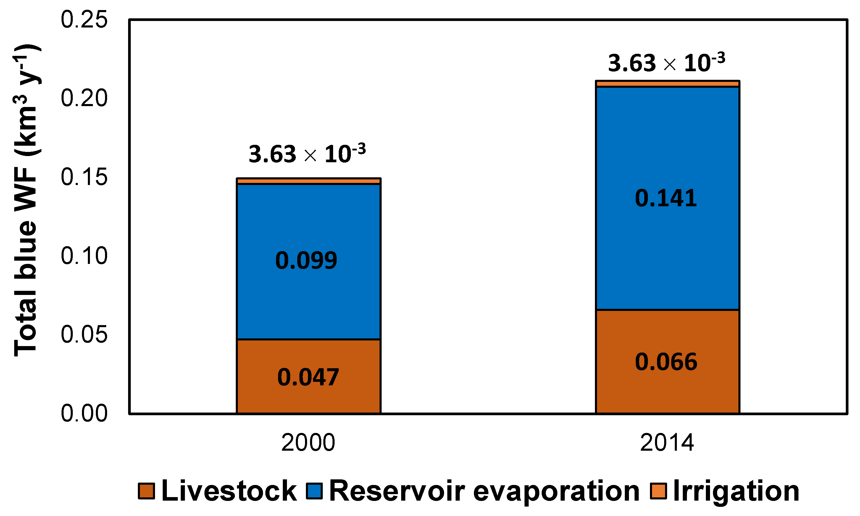
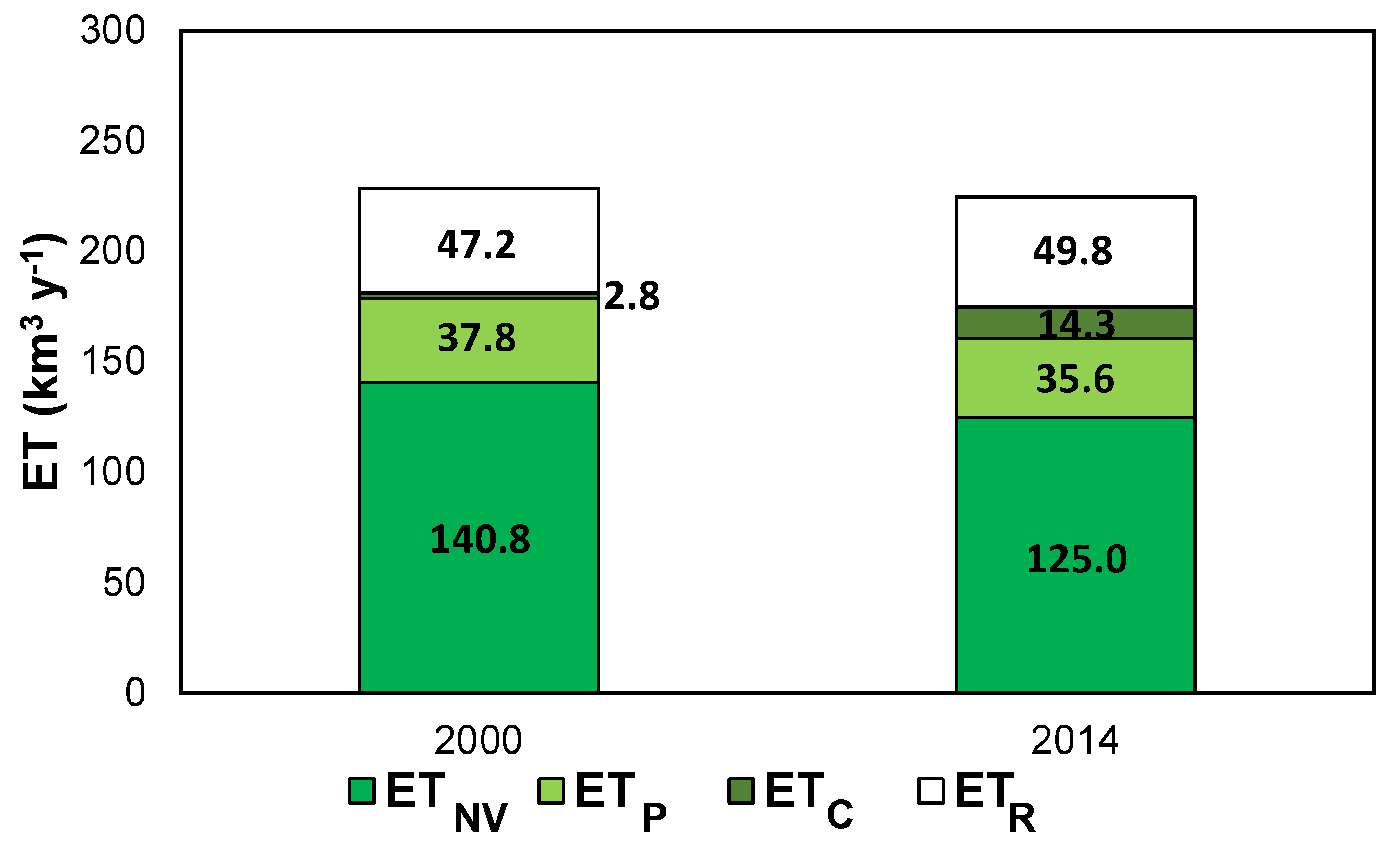
3.1. Past and Future Water Footprints

Between 2000 and 2014, the sum of cropland and pasture areas increased 31% from 4.7 Mha to 6.2 Mha. Changes in the consumption of blue water expressed by the total blue WF increased from 0.153 km³ y⁻¹ in 2000 to 0.218 km³ y⁻¹ in 2014 (Figure 2). The blue WF was dominated by agriculture, representing 97% of total water use, followed by domestic and industrial uses (Table S5). Water evaporation from small farm reservoirs represented 66% of total agricultural blue WF in 2000, and 67% in 2014, followed by livestock drinking (respectively 32% and 31%) and irrigation (2% of total consumption in both years) (Figure 2). Between 2000 and 2014, the total area of small farm reservoirs increased 37% from 6914 ha to 9463 ha of water, leading to a total evaporation of 0.099 km³ y⁻¹ and 0.141 km³ y⁻¹, respectively. Domestic blue water consumption computed here was similar to values from ANA [26], which reported 3.47 10⁻³ km³ y⁻¹ in 2007, while our industrial consumption estimates were three orders of magnitude smaller than the 3.55 10⁻² km³ y⁻¹ reported for 2007 [26]. Differences in industrial uses are primarily attributed to our separation of confined livestock from industry, as well as our focus on extractive and transformative industries. Combining livestock and industrial water consumptive uses raised our computed values closer to those reported by ANA [26]. The total blue WF increased with larger human and livestock populations in 2030 and 2050. In 2030, agricultural water use nearly doubled to 0.258 km³ y⁻¹, while the combined industrial and domestic uses increased to 9.90 10⁻³ km³ y⁻¹ (Table S5). In 2050, agricultural water use increased to 0.517 km³ y⁻¹ and 0.391 km³ y⁻¹ in the BAU and GOV scenarios, respectively. In the case of cattle confinement and early season soybean irrigation (GOV_RCP8.5), consumption rose to 3.81 km³ y⁻¹.

Agricultural expansion resulted in an increase in the total green WF of agriculture (as ET_AG) from 40.6 km³ y⁻¹ in 2000 to 49.9 km³ y⁻¹ in 2014 (Table S7). This change was led by cropland ET which increased from 7 to 29% of ET_AG, while pasture dropped from 93 to 71% of ET_AG in the same time period (Figure 3). The increase in green WF occurred at the expense of the natural vegetation whose contributions to ET dropped 11% between 2000 and 2014 due to a decrease in forest cover by roughly 1.4 Mha. Changes in ET_AG and ET_NV obtained through the bottom-up approach were similar to results from Silvério et al. [9] (Table S7). Further deforestation for agriculture in 2030 and 2050 increased ET of non-forested areas to 188.6 km³ y⁻¹ and 209.6 km³ y⁻¹ for the BAU scenarios in 2030 and 2050 respectively, and 147.2 km³ y⁻¹ and 147.3 for the GOV scenarios (average climate change scenarios) (Figure S4, Table S8).

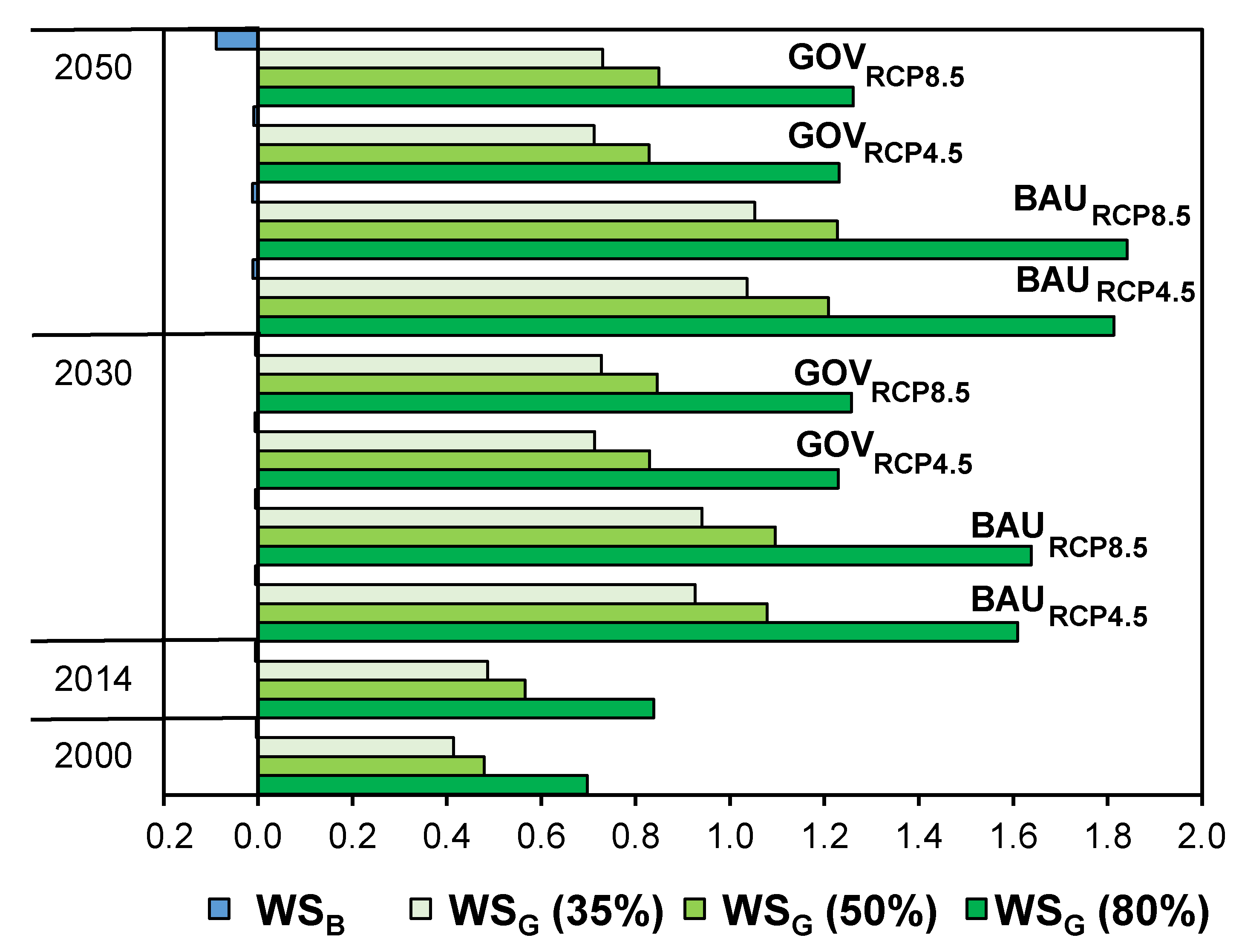
3.2. Blue and Green Water Availability and Scarcity

Annual runoff decreased from 74.9 km³ y⁻¹ to 70.4 km³ y⁻¹ between 2000 and 2014 (Table S6), which, when considering environmental flow requirements, left 43.4 km³ y⁻¹ (in 2000) and 40.8 km³ y⁻¹ (in 2014) of blue water available in the basin. The decrease in annual runoff followed the decline in precipitation from 1999 mm y⁻¹ in 2000 to 1934 mm y⁻¹ in 2014 (Table S6). When considering 3-month windows, the decrease in runoff was more prominent in the December–February period where values decreased from 20.7 km³ 3-month⁻¹ in 2000–2001 to 14.3 km³ 3-month⁻¹ in 2014–2015 (Table S6), which we relate to a reduction in September–November precipitation from 519 mm 3-months⁻¹ in 2001 to 447 mm 3-months⁻¹ in 2014.

The combination of deforestation and climate change in the scenarios generally increased runoff by 2% in 2030 when compared to 2000 (GOV_RCP4.5), and by 8% in 2050 (BAU_RCP4.5) despite a reduction in precipitation (Table S6). The GOV_RCP8.5 scenario was the only exception with a decrease in runoff of 1% in 2050 for a precipitation decline to 1952 mm y⁻¹. Focusing on climate change effects alone, runoff with potential natural vegetation cover in the basin decreased from 69.8 km³ y⁻¹ in 2000 to 64.1 km³ y⁻¹ in 2014, 67.9–69.1 km³ y⁻¹ in 2030 and 65.7–69.0 km³ y⁻¹ in 2050 (Table S6). Inter-annual changes in runoff were apparent when considering 3-month windows: runoff generally increased at the beginning of the wet season (September–November, +13–20%), before decreasing at the end of the wet season (December–February, ‒62–71%). Dry season runoff increased between 22% and 52% in the June to August periods when compared to 2000 (Table S6).

Land contributions to ET in the basin were similar between 2000 (279.0 km³ y⁻¹) and 2014 (272.0 km³ y⁻¹) (Table S8). In 2000, forests represented 50–69% of contributions (bottom-up and top-down estimates), while agriculture represented 15% (bottom-up estimates) (Tables S7 and S8). In 2014, these values changed to 46–63% and 18% for forests and agriculture, respectively. Total land contributions to ET dropped by up to 4% in the GOV_RCP4.5 scenario in 2030 and both BAU_RCP4.5 and GOV_RCP4.5 scenarios in 2050 (Table S8, Figure S4) with differences in contributions based on forest cover. Forests in the GOV_RCP4.5 scenario provided 122.9 km³ y⁻¹ and 122.5 km³ y⁻¹ of ET in 2030 and 2050, respectively. In contrast, BAU_RCP4.5 showed a reduction of natural vegetation ET from 82.1 km³ y⁻¹ in 2030 to 60.0 km³ y⁻¹ in 2050 as a result of reduced forest cover (Table S8, Figure S4).

Annual blue water scarcity values were less than 0.10 (Figure 4) with the largest value recorded in the GOV_RCP8.5 scenario in 2050 (0.09). Inter-annual values increased to 0.65 for the GOV_RCP8.5 scenario between September and November 2050 due to early soybean planting and irrigation (with inter-annual blue water scarcity values ≤0.03 the rest of the year). Annual green water scarcity values changed according to deforestation scenarios, but also due to restrictions placed on the allocation of natural vegetation. Between 2000 and 2014, green water scarcity was at least “within sustainable limits” (WS_G < 0.50) when considering the bottom-up approach, moving closer to “threat” conditions (0.5 < WS_G < 1) in the top-down approach (Figure 4). In 2030 and 2050, green water scarcity values increased to 1.1 in the BAU-2050 scenario considering 35% of natural vegetation allocated to the basin, and beyond 1.2 when allocation increased to 50% and 80%. In the same time period, the GOV scenario maintained WS_G < 1 with a 50% allocation to natural vegetation, but moved to “unsustainable conditions” in both 2030 and 2050 when allocating 80% of the basin allocated to natural vegetation (Figure 4).

4. Discussion

4.1. Agricultural Development and Water Resources

Agriculture was found to be the largest contributor to the total blue WF in the basin, with livestock water consumption for drinking and from reservoir evaporation representing the largest component. Water allocated to livestock production systems in 2014 was equivalent to the consumption of 2.3 million people connected to the municipal system. Animal population in the basin was historically led by cattle, but pig and chicken production have increased in recent years [16], effectively increasing water consumption and the water supply needed for production. Chickens and pigs are typically raised in confined facilities in Mato Grosso and, therefore, rely on surface or groundwater pumped for drinking water. In contrast, cattle in Mato Grosso rely on small reservoirs whose evaporation constitutes more than half of agricultural blue water consumption. Some of these reservoirs are constructed from impoundments of small streams, which contribute to stream warming with potential effects on stream chemistry [29] and hydrologic connectivity [56]. The regional effects of these reservoirs on hydrology remain relatively unexplored in Southern Amazonia.

The replacement of natural vegetation by cropland and pasture was illustrated by an increase in green water appropriation in the basin. We report a decline in pasture area in 2014 compared to 2000, which, when combined with increasing cattle population, led to an increase in cattle density (0.57 cattle ha⁻¹ in 2001 to 0.97 cattle ha⁻¹ in 2015), following general trends in the state of Mato Grosso [40]. The replacement of deep rooted natural vegetation with shallow-rooted crops and pasture affects radiation partitioning by decreasing latent heat and increasing sensible heat fluxes [15]. These changes in radiation partitioning have important consequences on surface temperatures. Silvério et al. [9] showed that cropland and pasture surface temperatures in the XBMT were 6.4 °C and 4.3 °C greater than forests. As a result, deforestation between 2000 and 2010 led to an average basin temperature increase of 0.3 °C on top of the 1.7 °C increase that had occurred because of deforestation prior to 2000 [9]. The Xingu Indigenous Park located in the heart of the basin (Figure 1) showed surface temperatures 3 °C lower inside the protected area compared to the rest of the basin [57]. Such effects illustrate the importance of maintaining natural forest cover.

Water consumption in future agricultural production varied substantially based on the conditions of production, which include land expansion and intensification. Our evaluation of two agricultural expansion scenarios highlights the extent of future green water appropriation from rain-fed agriculture which carries consequences for the carbon and water cycles [37]. Agricultural intensification for both crops and livestock requires either more efficient use of green water on current land, a reallocation of green water resources for production (e.g., cropland expansion into pasture), additional blue water consumption from irrigation, or a combination of the above [15]. Under current production practices, the onset of the wet season dictates when (or if) a second crop (typically maize) could be planted [39,58]. Farmers may plant soybean earlier in the season (e.g., in September) and irrigate fields until the onset of the wet season (e.g., approximately 16 October 2007 in the basin [58]) to allow for earlier planting and harvesting of maize, and the potential success of two crops. Under this strategy, farmers could also add a third irrigated dry season crop (e.g., bean) leading to additional blue water consumption [40].

Similarly, future cattle production may include additional confinement as a strategy to free pasture for cropland expansion. A larger cattle population means greater appropriation of both green water (through feed) and blue water (through drinking, small farm reservoirs, cleaning of pens, etc.) [40]. Confinement could also move towards the use of blue water sources other than those stored in small farm reservoirs (e.g., groundwater), in which case the total blue WF of cattle could drop. However, this apparent efficiency has to be assessed considering the use of reservoirs in the long term, or their possible decommissioning or alternative use in other production systems (e.g., as irrigation). Potential water savings through efficiencies in the cattle production system (e.g., reservoir evaporation management) could also reduce the blue WF of cattle to allow greater water availability downstream [40,59].

Since 2000, the state of Mato Grosso increased meat production for both domestic consumption and international exports. The amount of water used for production is therefore virtually transferred to consumers within and outside of Brazil [60] (80% of Brazilian production is consumed within the country according to the Bovine Support Fund (FABOV as the Portuguese acronym) [61]). Between 2000 and 2014, Mato Grosso meat exports rose from 27,000 tons to 387,000 tons [62], thereby increasing the amount of water consumed regionally for foreign export, along with soybean commodities [37]. For instance, 27% of Europe’s virtual water imports between 2006 and 2015 came from soybean trade [63].

The selection of future production systems proposed through our scenarios can therefore change the resource appropriation for regional production, which already carries nutrient and carbon footprints that can be allocated to consumers [37]. This connection between consumption and production centers has inspired demand-side management of water use through the supply chain. For instance, Vanham et al. [64] estimated the WF of different European diets and their implications for water resources. Supply chain interventions in the region have been motivated by deforestation and climate change implications though both the “Soybean Moratorium” or the “Cattle Agreement” [65], but could also include water resources given the close link between land and water resources management in agricultural production systems [15].

4.2. Changes in Water Scarcity with Land and Water Management

Activities in the basin through present day were found to be within blue water sustainable limits. Green water resources, however, were within sustainable limits under specific conditions only. Inter-annual blue water scarcity moved closer to “moderate” under irrigation expansion and cattle confinement, reflecting the potential vulnerability of the basin to dry season agricultural water use. A total of 234 irrigation pivots covering almost 28,000 ha were identified in the municipalities overlapping XBMT [66] and expansion could increase given the 10 Mha irrigation capacity estimated for Mato Grosso [67]. Similarly, the developed reservoir capacity for cattle is a measure to ensure continued drinking water in the dry season when animals may need more water due to meteorological conditions [68]. This water consumed for agricultural production is then unavailable for other human and ecosystem uses in the greater Xingu River Basin, and may affect wetlands or hydroelectric power production [14,28]. Water rationing has already taken place as a result of drought (e.g., 2005) and the lack of infrastructure to cope with low water levels, particularly in the Xingu Headwaters [26]. We therefore expect future water use for irrigation and cattle to also come from additional sources (e.g., surface and groundwater sources) should water become scarce in the dry season. Consequently, both intensification of soybean and cattle production should carefully observe the effects on future water scarcity in the basin in agricultural management plans.

While policies have mostly focused on maintaining forest cover to protect biodiversity and reduce greenhouse gas emissions, these policies can also play a role in maintaining sustainable water resource use. The sustainable limits that we calculated relied on our estimate of water availability (WA_B, WA_G) which depended in turn on the interaction of land and water management initiatives. We found that natural runoff (i.e., runoff without any consumption activity, affecting WA_B) would change in 2030 and 2050 as a result of deforestation and climate change, while total land ET (affecting WA_G) responded directly to the allocation of land to natural vegetation cover, with a feedback on natural runoff. Changes in the natural runoff resulting from deforestation and climate change have already been measured in the region. For example, the 15% forest cover loss between 1971 and 2010 in the Xingu River Basin led to a 6% increase in runoff, while climate variability led to a 2% decrease in precipitation and 14% decrease in runoff [28]. Groundwater is known to act as a buffer in the basin, particularly in the dry season when runoff could diminish due to an extended dry season ET [69]. Changes in water availability can therefore be affected by the amount of deforestation in the basin represented by the BAU and GOV scenarios also guided by Brazilian Federal law.

The determination of green water scarcity assumed an increasing amount of land allocated to natural vegetation in the basin based on natural vegetation cover mandated by the Federal Forest Code [47]. As such, our interpretation of green water scarcity was based on the amount of vegetation cover lost in the basin in relation to Federal thresholds, which vary by biome from 35% (Cerrado savanna) to 80% (Amazon forest). For instance, in 2014, green water scarcity was within “threat” conditions when allocating 80% of the basin to natural vegetation (based on ET in the 2000 hydrologic year as described in Section 2.3.3). These “threat” conditions mean that from the total amount of green water available in the XBMT (represented by total ET, ET_T), the amount that could be put to use for agricultural production approached the limits mandated by the retention of natural vegetation cover (80%). Even in a restrictive deforestation scenario (GOV), green water appropriation would be unsustainable unless the policy goal for natural vegetation cover were reduced from 80% to 50%, in which case the basin’s green water scarcity changes from “unsustainable” to “threat” conditions. The XBMT is located within the Amazon and Cerrado biomes, which have different mandatory levels of natural vegetation cover based on whether a property was within the Cerrado (35%), Amazon (80%), or the transition zone between the two (50%). We therefore conclude, that future green water appropriation will, at best, remain under “threat” conditions considering both a restrictive deforestation scenario (GOV) and a 50% natural vegetation cover. This analysis, however, does not include potential indirect land use change that might occur outside the limits of the basin [2,39,70].

The increase in green water appropriation by cropland and pasture from natural vegetation through agricultural extensification, was previously observed in the basin [9], at the Mato Grosso state level [10], and the Cerrado [3]. These studies show that land use change can impact the water cycle by returning less water vapor to the atmosphere when compared to natural vegetation with a potential reduction on regional precipitation [71,72]. Regional precipitation is sourced from green water resources as opposed to ocean evaporation [73], such that land use change may, in turn, affect water availability within and outside the basin [11,12,13,74]. This so-called “moisture recycling”, however, is also expected to be affected by the expansion of irrigation practices which could transfer additional water vapor to the atmosphere in the dry season when regional recycling is enhanced [75].

4.3. Response Formulation and Study Limitations

Our scenarios represent two possible agricultural production options [15] considering agriculture remains the largest water consumer in the basin. These options reflected whether agricultural intensification relied on cropland expansion into pasture (the Green Option), or whether cropping frequency and livestock confinement becomes more widespread in the future (the Blue Option) (

Table 2. Summary of effects and responses for two agricultural production options focused on production intensification in the Xingu Basin of Mato Grosso.

Description	The Green Option		The Blue Option
	Crops	Cattle	Crops	Cattle
Strategy	Increase production by increasing cropped area	Intensify production on current land	Increase crop frequency (triple cropping)	Intensify production through confinement
Land use	Expansion of crops into pastureland	Concentration of cattle on current and more productive pastureland	Cropland expansion into pastureland	Increase confinement of cattle
Water use	Reallocate water from cattle to cropland	Reduce water use for a more productive pasture; Feed sourced off-farm (virtual water transfers); Increase small reservoir capacity	Use irrigation for early soybean planting and include a dry season irrigated crop	Increase small reservoir capacity; Supplemental drinking from surface and groundwater in confined systems
Effects on blue water use and scarcity	Blue water consumption increases with animal population, reservoir evaporation and groundwater use, but remains within sustainable limits		Blue water consumption approaches sustainable limits in the dry season with potential effects on downstream water availability
Effects on green water use and scarcity	Green water use increases for crops and decreases for pasture keeping green water scarcity constant; Green water availability may change in the long-term due to local (land use) and global (CO2 emissions) climate change and additional evaporation from farm reservoirs increase water vapor flows to the atmosphere; Changes in precipitation affect blue and green water availability in- and outside the basin.		Green water use increases for crops and decreases for pasture keeping green water scarcity constant; Green water availability may change in the long-term due to local (land use) and global (CO2 emissions) climate change but additional ET from crop irrigation and farm reservoirs increase water vapor flows to the atmosphere; Changes in precipitation affect blue and green water availability in- and outside the basin.
Water management considerations	Improve efficiency of blue water use, especially the reduction of evaporation from farm reservoirs; Consider effects of land (precipitation and runoff) beyond the basin; Integrate land and water policies.		Improve efficiencies in blue water use for irrigation and confined livestock; Groundwater management or the use of old farm reservoirs could be used without affecting runoff; Consider effects of land use on water availability, especially the effects of additional water vapor supply to the atmosphere.

). Further appropriation of green water from either natural vegetation or pasture depends on land use policies and incentives (e.g., Federal Forest Code, Protective Areas, etc.), while blue water use depends on water management, which has generally focused on human rather than ecosystem requirements [14]. Both options have consequences for future water availability: continued reduction in natural vegetation cover, which is accompanied by reduced water vapor supply to the atmosphere could also affect terrestrial ecosystems that rely on precipitation for ecosystem functioning [15], while dry season water consumed in intensified livestock and irrigation systems could impact aquatic ecosystems downstream.

Regional water resources planning requires that connectivity of the water cycle among basins and biomes be maintained in order to secure future water availability within the basin and beyond. Water resources management options should consider upstream rain-fed agriculture and small farm reservoirs and their effects on downstream hydroelectric power. Currently, large hydropower dams (>10 MW) require environmental licenses and impact assessment studies, while smaller dams do not [14], suggesting possible conflicts between up- and downstream water uses. As 22% and 48% of evaporation in the Xingu and Amazon Basins, respectively, return to the same basins as precipitation [76,77], land and water management in a basin should go beyond its physical boundary. So far, effects of land use change on moisture recycling has been absent in water management, in part, due to the difficulty to connect precipitation source and sink regions in governance [78].

Water management strategies should also include green and blue water resource use efficiency gains at the field level. For instance, small farm reservoir management should strive to reduce total evaporation [15,59], especially when combining livestock confinement with the widespread use of irrigation for soybean planted at the end of the dry season (as described in our Blue Option). Moreover, green water use should attempt to improve transpiration over evaporation [15], while irrigation should be used efficiently. These actions depend on each individual farmer, their production systems, and the available training for capacity building of such options. For instance, the recent increase of cattle density on the current pastureland relied on increased pasture productivity with the potential to reduce the amount of water for feed [40]. However, such an initiative has been difficult to implement in the region [79], and the financial returns of increased cattle density still depend strongly on price fluctuations in the beef market [80].

Our study focused on environmental aspects related to water quantity, not social nor economic implications of water consumption, nor the effects of water quality on scarcity through the grey WF. As the largest water consuming sector in the basin, agriculture likely carries the greatest impacts both socially and economically. Some studies have made strong connections between agricultural development and human and economic development [5,81]. The effects on water quality resulting from widespread fertilizer application in the XBMT have been inconclusive thus far with respect to eutrophication [82], while few studies have investigated the effects of pesticides on water quality in Southern Amazonia [81]. The increase in livestock confinement for both swine and chicken production suggest additional on-farm waste management, which could also affect water quality and were not considered in this study.

Results of this study relied on the accuracy of the IBIS model to represent the water cycle from land use maps. Our bottom-up approach relied on maps obtained from Landsat imagery which were used to infer runoff, and ET using average land use system values derived from previously published results. The derived runoff and ET results were used exclusively for the 2000–2001 and 2014–2015 period and were close to the observations (see Supplemental Material). Our top-down approach used for the 2030–2031 and 2050–2051 periods relied on the assumption that cropland and pasture ET were equal. Cropland and pasture ET can differ by almost 100 mm (see Table S1) suggesting a potential overestimation of agricultural land ET (Figure S4). A reduction in agricultural ET would increase the estimated runoff and decrease agricultural green water consumption. These changes would have a small effect on our annual blue water scarcity values, and limited effect on our green water scarcity values which were more sensitive to the allocation of ET to natural vegetation (ET_RNV).

Our results used IBIS to infer natural runoff under deforestation and climate change scenarios, which do not include the feedbacks of water consumption activities. First, blue water scarcity values were estimated based on the appropriation of runoff as the blue water source. The currently reported XBMT water use is made up of only 20% of surface water with the remainder coming from deep and shallow wells [26]. We therefore expect future dry season blue water scarcity limits to take longer to reach as a result of groundwater extraction in the case of soybean irrigation and cattle confinement. Groundwater in Southeastern Amazonia is deep and known to also feed streams in the Xingu Headwaters [83,84]. Therefore, the effects of extensive groundwater extraction could only partially contribute to blue water scarcity, unlike other regions [85]. Our results, however, are still expected to represent a general trend towards greater water scarcity given the large contribution of drinking water for cattle and evaporation from small farm reservoirs which was entirely attributed to surface water.

In this case we also expect groundwater storage to act as a blue water source available to alleviate agricultural water demand in cases of domestic, industrial consumption and additional demand from confined livestock and irrigated agriculture which merit further investigation. It is important to note that the inter-annual water scarcity values were based on 3-month means of natural runoff obtained from IBIS, which we found to be close to observed values between September and November when blue water scarcity was its greatest in 2050.

Moisture recycling feedbacks resulting from reduced vegetation cover and an expanding small farm reservoir network were not included in our estimate of both long-term green and blue water availability and, therefore, water scarcity indicators. A reduction in precipitation as a result of land use change would reduce green water availability in the basin and therefore increase the magnitudes of our estimates towards more unsustainable limits. Similarly, reduced precipitation in the basin can further affect runoff at the regional scale [14], thereby increasing blue water scarcity as estimated here. Both of these limitations, therefore suggest that our results represent mainly a conservative estimate of the effects described in this study.

5. Conclusions

The application of the WFSA revealed the importance of the agricultural sector for future land and water management initiatives in the XBMT. Our study has also provided an important case for estimating blue and green water scarcities in the context of land use change, climate change and agricultural production scenarios. Agricultural expansion between 2000 and 2015 led to conditions under which green water scarcity moved towards “threat” conditions, while blue water resources remained within sustainable limits. The evaluation of two water resource use options for agricultural intensification confirmed the importance of land use policies in further reducing deforestation as a driver for intensifying agricultural production in the basin. Future cropland expansion can rely on further green water appropriation by expanding onto pasture, while cattle confinement and cropland irrigation for increased cropping frequency have the potential of bringing the basin towards dry season sustainable limits. Future studies should consider the role of small farm reservoirs and irrigation in the water cycle to identify their importance for regional groundwater storage, downstream blue water availability, and also for large scale moisture recycling and the atmospheric water balance.

References

1. Simon, M.F.; Garagorry, F.L. The expansion of agriculture in the Brazilian Amazon. Environ. Conserv. 2006, 32, 203. [Google Scholar] [CrossRef]
2. Barona, E.; Ramankutty, N.; Hyman, G.; Coomes, O.T. The role of pasture and soybean in deforestation of the Brazilian Amazon. Environ. Res. Lett. 2010, 5, 024002. [Google Scholar] [CrossRef]
3. Spera, S.A.; Galford, G.L.; Coe, M.T.; Macedo, M.N.; Mustard, J.F. Land-use change affects water recycling in Brazil’s last agricultural frontier. Glob. Chang. Biol. 2016, 22, 3405–3413. [Google Scholar] [CrossRef] [PubMed]
4. Macedo, M.N.; DeFries, R.S.; Morton, D.C.; Stickler, C.M.; Galford, G.L.; Shimabukuro, Y.E. Decoupling of deforestation and soy production in the southern Amazon during the late 2000s. Proc. Natl. Acad. Sci. USA 2012, 109, 1341–1346. [Google Scholar] [CrossRef] [PubMed]
5. Richards, P.; Pellegrina, H.; VanWey, L.; Spera, S. Soybean Development: The Impact of a Decade of Agricultural Change on Urban and Economic Growth in Mato Grosso, Brazil. PLoS ONE 2015, 10, e0122510. [Google Scholar] [CrossRef] [PubMed]
6. Davidson, E.A.; de Araújo, A.C.; Artaxo, P.; Balch, J.K.; Brown, I.F.; Bustamante, M.M.C.; Coe, M.T.; DeFries, R.S.; Keller, M.; Longo, M.; et al. The Amazon basin in transition. Nature 2012, 481, 321–328. [Google Scholar] [CrossRef] [PubMed]
7. Galford, G.L.; Melillo, J.; Mustard, J.F.; Cerri, C.E.P.; Cerri, C.C. The Amazon Frontier of Land-Use Change: Croplands and Consequences for Greenhouse Gas Emissions. Earth Interact. 2010, 14, 1–24. [Google Scholar] [CrossRef]
8. Coe, M.T.; Costa, M.H.; Soares-Filho, B.S. The influence of historical and potential future deforestation on the stream flow of the Amazon River—Land surface processes and atmospheric feedbacks. J. Hydrol. 2009, 369, 165–174. [Google Scholar] [CrossRef]
9. Silvério, D.V.; Brando, P.M.; Macedo, M.N.; Beck, P.S.A.; Bustamante, M.; Coe, M.T. Agricultural expansion dominates climate changes in southeastern Amazonia: The overlooked non-GHG forcing. Environ. Res. Lett. 2015, 10, 104015. [Google Scholar] [CrossRef]
10. Lathuillière, M.J.; Johnson, M.S.; Donner, S.D. Water use by terrestrial ecosystems: Temporal variability in rainforest and agricultural contributions to evapotranspiration in Mato Grosso, Brazil. Environ. Res. Lett. 2012, 7, 024024. [Google Scholar] [CrossRef]
11. António Sumila, T.C.; Pires, G.F.; Fontes, V.C.; Costa, M.H. Sources of Water Vapor to Economically Relevant Regions in Amazonia and the Effect of Deforestation. J. Hydrometeorol. 2017, 18, 1643–1655. [Google Scholar] [CrossRef]
12. Oliveira, L.J.C.; Costa, M.H.; Soares-Filho, B.S.; Coe, M.T. Large-scale expansion of agriculture in Amazonia may be a no-win scenario. Environ. Res. Lett. 2013, 8, 024021. [Google Scholar] [CrossRef]
13. Stickler, C.M.; Coe, M.T.; Costa, M.H.; Nepstad, D.C.; McGrath, D.G.; Dias, L.C.P.; Rodrigues, H.O.; Soares-Filho, B.S. Dependence of hydropower energy generation on forests in the Amazon Basin at local and regional scales. Proc. Natl. Acad. Sci. USA 2013, 110, 9601–9606. [Google Scholar] [CrossRef] [PubMed]
14. Castello, L.; Macedo, M.N. Large-scale degradation of Amazonian freshwater ecosystems. Glob. Chang. Biol. 2016, 22, 990–1007. [Google Scholar] [CrossRef] [PubMed]
15. Lathuillière, M.J.; Coe, M.T.; Johnson, M.S. A review of green- and blue-water resources and their trade-offs for future agricultural production in the Amazon Basin: What could irrigated agriculture mean for Amazonia? Hydrol. Earth Syst. Sci. 2016, 20, 2179–2194. [Google Scholar] [CrossRef]
16. IBGE. Banco de Dados Agregados. Available online: www.sidra.ibge.gov.br/ (accessed on 1 June 2016).
17. Hoekstra, A.Y.; Chapagain, A.K.; Aldaya, M.M.; Mekonnen, M.M. The Water Footprint Assessment Manual; Earthscan: London, UK, 2011; ISBN 9781849712798. [Google Scholar]
18. Chenoweth, J.; Hadjikakou, M.; Zoumides, C. Quantifying the human impact on water resources: A critical review of the water footprint concept. Hydrol. Earth Syst. Sci. 2014, 18, 2325–2342. [Google Scholar] [CrossRef] [Green Version]
19. Quinteiro, P.; Ridoutt, B.G.; Arroja, L.; Dias, A.C. Identification of methodological challenges remaining in the assessment of a water scarcity footprint: A review. Int. J. Life Cycle Assess. 2017. [Google Scholar] [CrossRef]
20. Hoekstra, A.Y. Water Footprint Assessment: Evolvement of a New Research Field. Water Resour. Manag. 2017, 31, 3061–3081. [Google Scholar] [CrossRef]
21. Falkenmark, M.; Rockström, J. The New Blue and Green Water Paradigm: Breaking New Ground for Water Resources Planning and Management. J. Water Resour. Plan. Manag. 2006, 132, 129–132. [Google Scholar] [CrossRef]
22. Mekonnen, M.M.; Hoekstra, A.Y. Four billion people facing severe water scarcity. Sci. Adv. 2016, 2, e1500323. [Google Scholar] [CrossRef] [PubMed]
23. Hoekstra, A.Y.; Mekonnen, M.M.; Chapagain, A.K.; Mathews, R.E.; Richter, B.D. Global Monthly Water Scarcity: Blue Water Footprints versus Blue Water Availability. PLoS ONE 2012, 7, e32688. [Google Scholar] [CrossRef] [PubMed]
24. Miguel Ayala, L.; van Eupen, M.; Zhang, G.; Pérez-Soba, M.; Martorano, L.G.; Lisboa, L.S.; Beltrao, N.E. Impact of agricultural expansion on water footprint in the Amazon under climate change scenarios. Sci. Total Environ. 2016, 569–570, 1159–1173. [Google Scholar] [CrossRef] [PubMed]
25. Schyns, J.F.; Hoekstra, A.Y.; Booij, M.J. Review and classification of indicators of green water availability and scarcity. Hydrol. Earth Syst. Sci. 2015, 19, 4581–4608. [Google Scholar] [CrossRef]
26. ANA. Plano Estratégico de Recursos Hídricos dos Afluentes da Margem Direita do Rio Amazonas; Agência Nacional de Águas: Brasilia, Brazil, 2013. [Google Scholar]
27. Velasquez, H.Q.C.; Bernasconi, P. Fique por Dentro: A Bacia do Rio Xingu em Mato Grosso; Instituto Socioambiental, Instituto Centro de Vida: São Paulo, Brazil, 2010. [Google Scholar]
28. Panday, P.K.; Coe, M.T.; Macedo, M.N.; Lefebvre, P.; Castanho, A.D.d.A. Deforestation offsets water balance changes due to climate variability in the Xingu River in eastern Amazonia. J. Hydrol. 2015, 523, 822–829. [Google Scholar] [CrossRef]
29. Macedo, M.N.; Coe, M.T.; DeFries, R.; Uriarte, M.; Brando, P.M.; Neill, C.; Walker, W.S. Land-use-driven stream warming in southeastern Amazonia. Philos. Trans. R. Soc. B Biol. Sci. 2013, 368, 20120153. [Google Scholar] [CrossRef] [PubMed]
30. ANA. Hidroweb. Available online: http://hidroweb.ana.gov.br/ (accessed on 1 June 2016).
31. Foley, J.A.; Kucharik, C.J.; Polzin, D. Integrated Biosphere Simulator Model (IBIS), Version 2.5; ORNL DAAC: Oak Ridge, TN, USA, 2005. [Google Scholar]
32. Foley, J.A.; Prentice, I.C.; Ramankutty, N.; Levis, S.; Pollard, D.; Sitch, S.; Haxeltine, A. An integrated biosphere model of land surface processes, terrestrial carbon balance, and vegetation dynamics. Glob. Biogeochem. Cycles 1996, 10, 603–628. [Google Scholar] [CrossRef]
33. Kucharik, C.J.; Foley, J.A.; Delire, C.; Fisher, V.A.; Coe, M.T.; Lenters, J.D.; Young-Molling, C.; Ramankutty, N. Testing the performance of a dynamic global ecosystem model: Water balance, carbon balance, and vegetation structure. Glob. Biogeochem. Cycles 2000, 14, 795–825. [Google Scholar] [CrossRef]
34. Ramankutty, N.; Foley, J.A. Estimating historical changes in global land cover: Croplands from 1700 to 1992. Glob. Biogeochem. Cycles 1999, 13, 997–1027. [Google Scholar] [CrossRef]
35. Graesser, J.; Ramankutty, N. Detection of cropland field parcels from Landsat imagery. Remote Sens. Environ. 2017, 201, 165–180. [Google Scholar] [CrossRef]
36. Soares-Filho, B.S.; Nepstad, D.C.; Curran, L.M.; Voll, E.; Garcia, R.A.; Ramos, C.A.; McDonald, A.J.; Lefebvre, P.A.; Schlesinger, P. LBA-ECO LC-14 Modeled Deforestation Scenarios, Amazon Basin: 2002–2050; ORNL DAAC: Oak Ridge, TN, USA, 2013. [Google Scholar] [CrossRef]
37. Lathuillière, M.J.; Johnson, M.S.; Galford, G.L.; Couto, E.G. Environmental footprints show China and Europe’s evolving resource appropriation for soybean production in Mato Grosso, Brazil. Environ. Res. Lett. 2014, 9, 074001. [Google Scholar] [CrossRef]
38. Lathuillière, M.J.; Bulle, C.; Johnson, M.S. Land Use in LCA: Including Regionally Altered Precipitation to Quantify Ecosystem Damage. Environ. Sci. Technol. 2016, 50, 11769–11778. [Google Scholar] [CrossRef] [PubMed]
39. Spera, S.A.; Cohn, A.S.; VanWey, L.K.; Mustard, J.F.; Rudorff, B.F.; Risso, J.; Adami, M. Recent cropping frequency, expansion, and abandonment in Mato Grosso, Brazil had selective land characteristics. Environ. Res. Lett. 2014, 9, 064010. [Google Scholar] [CrossRef]
40. Lathuillière, M.J. Harmonizing Water Footprint Assessment for Agricultural Production in Southern Amazonia; The University of British Columbia: Vancouver, BC, Canada, 2018. [Google Scholar]
41. Mesa, D.; Muniz, E.; Souza, A.; Geffroy, B. Broiler-Housing Conditions Affect the Performance. Rev. Bras. Ciência Avícola 2017, 19, 263–272. [Google Scholar] [CrossRef]
42. Palhares, J.C.P. Pegada hídrica dos suínos abatidos nos Estados da Região Centro-Sul do Brasil. Acta Sci. Anim. Sci. 2011, 33, 309–314. [Google Scholar] [CrossRef]
43. IPCC. 2006 IPCC Guidelines for National Greenhouse Gas Inventories, Prepared by the National Greenhouse Gas Inventories Programme; Eggleston, S., Buendia, L., Miwa, K., Ngara, T., Tanabe, K., Eds.; IGES: Hayama, Japan, 2006. [Google Scholar]
44. FAO. Guidelines for Water Use Assessment of Livestock Production Systems and Supply Chains; Livestock Environmental Assessment and Performance (LEAP) Partnership: Rome, Italy, 2018. [Google Scholar]
45. Smakhtin, V.; Revenga, C.; Döll, P. A Pilot Global Assessment of Environmental Water Requirements and Scarcity. Water Int. 2004, 29, 307–317. [Google Scholar] [CrossRef]
46. Richter, B.D.; Davis, M.M.; Apse, C.; Konrad, C. A presumptive standard for environmental flow protection. River Res. Appl. 2012, 28, 1312–1321. [Google Scholar] [CrossRef]
47. Presidência da República, Casa Civil, Subchefia para Assuntos Jurídicos. Lei no 12.651, de 25 de maio de 2012; Presidência da República, Casa Civil, Subchefia para Assuntos Jurídicos: Brasilia, Brazil, 2012. [Google Scholar]
48. MAPA. Projeções do Agronegócio: Brasil 2015/16 a 2025/26 Projeções de Longo Prazo; Ministério da Agricultura, Pecuária e Abastecimento: Brasilia, Brazil, 2016. [Google Scholar]
49. R Core Team. R: A Language and Environment for Statistical Computing; R Foundation for Statistical Computing: Vienna, Austria, 2017. [Google Scholar]
50. Hijmans, R.J. Raster: Geographic Data Analysis and Modeling. R package Version 2.5-8. Available online: https://cran.r-project.org/package=raster (accessed on 1 June 2016).
51. Bivand, R.S.; Pebesma, E.; Gomez-Rubio, V. Applied Spatial Data Analysis with R, 2nd ed.; Springer: New York, NY, USA, 2013. [Google Scholar]
52. Pebesma, E.J.; Bivand, R.S. Classes and Methods for Spatial Data in R. R News 5 (2). Available online: https://cran.r-project.org/doc/Rnews/ (accessed on 1 June 2016).
53. Bivand, R.; Keitt, T.; Rowlinsgon, B. Rgdal: Bindings for the Geospatial Data Abstraction Library. R Package Version 1.2-7. Available online: https://cran.r-project.org/package=rgdal (accessed on 1 June 2016).
54. Bivand, R.; Lewin-Koh, N. Maptools: Tools for Reading and Handling Spatial Objects. R package version 0.9-2. Available online: https://cran.r-project.org/package=maptools (accessed on 1 June 2016).
55. Pierce, D. ncdf4: Interface to Unidata netCDF (Version 4 or Earlier) Format Data Files. R Package Version 1.16. Available online: https://cran.r-project.org/package=ncdf4 (accessed on 1 June 2016).
56. Callow, J.N.; Smettem, K.R.J. The effect of farm dams and constructed banks on hydrologic connectivity and runoff estimation in agricultural landscapes. Environ. Model. Softw. 2009, 24, 959–968. [Google Scholar] [CrossRef]
57. Coe, M.T.; Brando, P.M.; Deegan, L.A.; Macedo, M.N.; Neill, C.; Silvério, D.V. The Forests of the Amazon and Cerrado Moderate Regional Climate and Are the Key to the Future. Trop. Conserv. Sci. 2017, 10, 1–6. [Google Scholar] [CrossRef]
58. Arvor, D.; Dubreuil, V.; Ronchail, J.; Simões, M.; Funatsu, B.M. Spatial patterns of rainfall regimes related to levels of double cropping agriculture systems in Mato Grosso (Brazil). Int. J. Climatol. 2014, 34, 2622–2633. [Google Scholar] [CrossRef]
59. Baillie, C. Assessment of Evaporation Losses and Evaporation Mitigation Technologies for on Farm Water Storages across Australia. Coop. Res. Cent. Irrig. Futures Irrig. Matters Ser. 2008, 05/08, 1–52. [Google Scholar]
60. Da Silva, V.; de Oliveira, S.; Hoekstra, A.; Dantas Neto, J.; Campos, J.; Braga, C.; de Araújo, L.; Aleixo, D.; de Brito, J.; de Souza, M.; et al. Water Footprint and Virtual Water Trade of Brazil. Water 2016, 8, 517. [Google Scholar] [CrossRef]
61. FABOV. Diagnostico da Cadeia Produtiva Agroindustrial da Bovinocultura de Corte do Estado de Mato Grosso; Fundo de Apoio à Bovinocultura de Corte: Cuiabá, Mato Grosso, Brazil, 2007. [Google Scholar]
62. MAPA. Agrostat. Available online: http://indicadores.agricultura.gov.br/agrostat (accessed on 1 June 2016).
63. Ercin, A.E.; Chico, D.; Chapagain, A.K. Dependencies of Europe’s Economy on Other Parts of the World in Terms of Water Resources. Available online: http://waterfootprint.org/media/downloads/Imprex-D12-1_final.pdf (accessed on 1 June 2016).
64. Vanham, D.; Mekonnen, M.M.; Hoekstra, A.Y. The water footprint of the EU for different diets. Ecol. Indic. 2013, 32, 1–8. [Google Scholar] [CrossRef]
65. Nepstad, D.; McGrath, D.; Stickler, C.; Alencar, A.; Azevedo, A.; Swette, B.; Bezerra, T.; DiGiano, M.; Shimada, J.; Seroa da Motta, R.; et al. Slowing Amazon deforestation through public policy and interventions in beef and soy supply chains. Science 2014, 344, 1118–1123. [Google Scholar] [CrossRef] [PubMed]
66. ANA & Embrapa/CNPMS. Levantamento da Agricultura Irrigada por Pivôs Centrais no Brasil—ano 2014; ANA and Embrapa: Brasilia, Brazil, 2016. [Google Scholar]
67. FEALQ. Análise Territorial Para o Desenvolvimento da Agricultural Irrigada no Brasil; Fundação de Estudos Agrários Luiz de Queiros: Piracicaba, São Paulo, Brazil, 2014. [Google Scholar]
68. Palhares, J.C.P.; Morelli, M.; Junior, C.C. Impact of roughage-concentrate ratio on the water footprints of beef feedlots. Agric. Syst. 2017, 155, 126–135. [Google Scholar] [CrossRef]
69. Pokhrel, Y.N.; Fan, Y.; Miguez-Macho, G. Potential hydrologic changes in the Amazon by the end of the 21st century and the groundwater buffer. Environ. Res. Lett. 2014, 9, 84004. [Google Scholar] [CrossRef]
70. Noojipady, P.; Morton, C.D.; Macedo, N.M.; Victoria, C.D.; Huang, C.; Gibbs, K.H.; Bolfe, L.E. Forest carbon emissions from cropland expansion in the Brazilian Cerrado biome. Environ. Res. Lett. 2017, 12, 025004. [Google Scholar] [CrossRef]
71. Khanna, J.; Medvigy, D.; Fueglistaler, S.; Walko, R. Regional dry-season climate changes due to three decades of Amazonian deforestation. Nat. Clim. Chang. 2017, 7, 200–204. [Google Scholar] [CrossRef]
72. Zemp, D.C.; Schleussner, C.-F.; Barbosa, H.M.J.; Hirota, M.; Montade, V.; Sampaio, G.; Staal, A.; Wang-Erlandsson, L.; Rammig, A. Self-amplified Amazon forest loss due to vegetation-atmosphere feedbacks. Nat. Commun. 2017, 8, 14681. [Google Scholar] [CrossRef] [PubMed]
73. Wright, J.S.; Fu, R.; Worden, J.R.; Chakraborty, S.; Clinton, N.E.; Risi, C.; Sun, Y.; Yin, L. Rainforest-initiated wet season onset over the southern Amazon. Proc. Natl. Acad. Sci. USA 2017, 114, 8481–8486. [Google Scholar] [CrossRef] [PubMed]
74. Keys, P.W.; Wang-Erlandsson, L.; Gordon, L.J. Revealing Invisible Water: Moisture Recycling as an Ecosystem Service. PLoS ONE 2016, 11, e0151993. [Google Scholar] [CrossRef] [PubMed]
75. Bagley, J.E.; Desai, A.R.; Harding, K.J.; Snyder, P.K.; Foley, J.A. Drought and Deforestation: Has Land Cover Change Influenced Recent Precipitation Extremes in the Amazon? J. Clim. 2014, 27, 345–361. [Google Scholar] [CrossRef]
76. Berger, M.; van der Ent, R.; Eisner, S.; Bach, V.; Finkbeiner, M. Water Accounting and Vulnerability Evaluation (WAVE): Considering Atmospheric Evaporation Recycling and the Risk of Freshwater Depletion in Water Footprinting. Environ. Sci. Technol. 2014, 48, 4521–4528. [Google Scholar] [CrossRef] [PubMed]
77. van der Ent, R.J.; Savenije, H.H.G.; Schaefli, B.; Steele-Dunne, S.C. Origin and fate of atmospheric moisture over continents. Water Resour. Res. 2010, 46, 1–12. [Google Scholar] [CrossRef]
78. Keys, P.; Wang-Erlandsson, L.; Gordon, L.; Galaz, V.; Ebbesson, J. Approaching moisture recycling governance. Glob. Environ. Chang. 2017, 45, 15–23. [Google Scholar] [CrossRef]
79. Latawiec, A.E.; Strassburg, B.B.N.; Silva, D.; Alves-Pinto, H.N.; Feltran-Barbieri, R.; Castro, A.; Iribarrem, A.; Rangel, M.C.; Kalif, K.A.B.; Gardner, T.; et al. Improving land management in Brazil: A perspective from producers. Agric. Ecosyst. Environ. 2017, 240, 276–286. [Google Scholar] [CrossRef]
80. Garcia, E.; Ramos Filho, F.; Mallmann, G.; Fonseca, F. Costs, Benefits and Challenges of Sustainable Livestock Intensification in a Major Deforestation Frontier in the Brazilian Amazon. Sustainability 2017, 9, 158. [Google Scholar] [CrossRef]
81. Arvor, D.; Tritsch, I.; Barcellos, C.; Jégou, N.; Dubreuil, V. Land use sustainability on the South-Eastern Amazon agricultural frontier: Recent progress and the challenges ahead. Appl. Geogr. 2017, 80, 86–97. [Google Scholar] [CrossRef]
82. Neill, C.; Jankowski, K.; Brando, P.M.; Coe, M.T.; Deegan, L.A.; Macedo, M.N.; Riskin, S.H.; Porder, S.; Elsenbeer, H.; Krusche, A.V. Surprisingly Modest Water Quality Impacts From Expansion and Intensification of Large-Sscale Commercial Agriculture in the Brazilian Amazon-Cerrado Region. Trop. Conserv. Sci. 2017, 10, 1–5. [Google Scholar] [CrossRef]
83. Hayhoe, S.J.; Neill, C.; Porder, S.; McHorney, R.; Lefebvre, P.; Coe, M.T.; Elsenbeer, H.; Krusche, A.V. Conversion to soy on the Amazonian agricultural frontier increases streamflow without affecting stormflow dynamics. Glob. Chang. Biol. 2011, 17, 1821–1833. [Google Scholar] [CrossRef]
84. Pokhrel, Y.N.; Fan, Y.; Miguez-Macho, G.; Yeh, P.J.F.; Han, S.C. The role of groundwater in the Amazon water cycle: 3. Influence on terrestrial water storage computations and comparison with GRACE. J. Geophys. Res. Atmos. 2013, 118, 3233–3244. [Google Scholar] [CrossRef]
85. Gleeson, T.; Wada, Y.; Bierkens, M.F.P.; van Beek, L.P.H. Water balance of global aquifers revealed by groundwater footprint. Nature 2012, 488, 197–200. [Google Scholar] [CrossRef] [PubMed]
Figure 1. The Xingu Basin of Mato Grosso (XBMT) and its sub-basins: the Upper Xingu Basin (yellow) and the Xingu Headwaters (green) with the main rivers and the location of the discharge measurement station used for validation [30]. The inset shows the position of XBMT (black) in relation to the Xingu River Basin (black outline) and the state of Mato Grosso (grey).
Water 10 00349 g001
Figure 2. Total blue Water Footprint (WF) of agriculture in the Xingu Basin of Mato Grosso for the 2000 and 2014 hydrologic years.
Water 10 00349 g002
Figure 3. Changes in contributions to evapotranspiration (ET) for natural vegetation (ETNV), pasture (ETP), cropland (ETC) and residual landscapes (ETR) in the Xingu Basin of Mato Grosso in the 2000, and 2014 hydrologic years (September–August). Values obtained through the bottom-up approach as described in the text.
Water 10 00349 g003
Figure 4. Annual blue (WSB) and green (WSG) water scarcities for the Xingu Basin of Mato Grosso in 2000 and 2014 hydrologic years, business-as-usual (BAU) and governance (GOV) deforestation scenarios considering Representative Concentration Pathways (RCP 4.5 and 8.5 W m−2) (Table 1). Values of WSG were obtained assuming that 35%, 50%, and 80% natural vegetation cover in the basin was maintained as described in the text.
Water 10 00349 g004