Assessing Impacts of Climate Change and Sea-Level Rise on Seawater Intrusion in a Coastal Aquifer


1
APEC Climate Center, 12 Centum 7-ro, Haeundae-gu, Busan 48058, Korea
2
Jeju Regional Headquarter, Seonsa-ro, Jeju-si 63318, Korea
*
Author to whom correspondence should be addressed.
Water 2018, 10(4), 357; https://doi.org/10.3390/w10040357
Submission received: 30 January 2018
/
Revised: 20 March 2018
/
Accepted: 21 March 2018
/
Published: 22 March 2018
Abstract
:The objectives of this study were to assess the climate change impacts on sea-level rise (SLR) and freshwater recharge rates and to investigate these SLR and freshwater recharge rates on seawater intrusion in coastal groundwater systems through the Saturated-Unsaturated Transport (SUTRA) model. The Gunsan tide gauge station data were used to project SLR based on polynomial regressions. Freshwater recharge rates were assumed as 10% of the projected annual precipitation under climate change. The Byeonsan2 groundwater monitoring well for seawater intrusion was selected for the study. A total of 15 scenarios, including the baseline period (2005–2015), were made based on SLR projections and estimated freshwater recharge rates. The changes in salinity relative to the baseline at the monitoring well for each scenario were investigated through the SUTRA model. From the scenario of 0.57 m SLR with a freshwater recharge rate of 0.0058 kg s−1, the largest salinity increase (40.3%) was simulated. We concluded that this study may provide a better understanding of the climate change impacts on seawater intrusion by considering both SLR and freshwater recharge rates.
1. Introduction
Global mean sea-level under Representative Concentration Pathway (RCP) 8.5 is projected to rise by 0.45–0.82 m from 1986–2005 to 2081–2100, while 0.32–0.70 m of the global mean sea level rise is projected by 2100 under RCP 4.5 [1]. For the Korean peninsula, sea-level rise (SLR) of 0.75 m under RCP 4.5 is estimated at the coast line in the East Sea by 2100, followed by the South Sea (0.58 m) and the West Sea 0.57 m [2]. Those under RCP 8.5 are 1.08 m for the East Sea, 0.72 m for the West Sea, and 0.70 m for the South Sea.
Several approaches have been used to assess SLR or sea-level acceleration (SLA) [3,4,5,6]. Breaker and Ruzmaikin [4] employed the ensemble empirical model decomposition (EEMD) method to estimate acceleration from 1855 to 2010 with the monthly averaged sea level data for San Francisco (CA, USA). They reported that SLA was 0.011 ± 0.003 mm yr−2 over the 157-year record of sea level. They also used polynomial regression for the SLA estimation and found that 0.013 mm yr−2, −0.0006 mm yr−2, and −0.023 mm yr−2 for the periods 1855–2011, 1900–2011, and 1925–2011, respectively. Eazer and Corlett [5] showed that SLA for Chesapeake Bay (USA) ranged from 0.05 to 0.10 mm yr−2 using Empirical Mode Decomposition and Hilbert-Huang Transformation [6]. Kim and Cho [7] reported that the average SLR around the Korean peninsula over the study period was 2.57 mm yr−1 and the average SLA 0.075 ± 0.026 mm yr−2 based on EEMD. They also found that 2.603 ± 0.0266 mm yr−1 and 0.114 ± 0.040 mm yr−2 for SLR and SLA, respectively, using polynomial regressions. Yoon [8] found that SLR around the Korean peninsula was higher the global mean SLR using a regression approach from tide gauge data.
Seawater intrusion has been frequently reported around the world: USA [9,10,11,12], Europe [13], Australia [14], China [15], India [16,17,18], Egypt [19], Bangladesh [20], and South Korea [21,22]. There have been many studies on the assessment of the impacts of SLR on seawater intrusion using various conceptual and mathematical models. Werner and Simmons [23] used a simple conceptual approach to assess seawater intrusion in coastal unconfined aquifers by SLR. Pool and Carrera [24] proposed a double pumping barrier system with two extraction wells combined with an inland well and a seaward well. The former was for pumping freshwater and the latter for seawater. They investigated the proposed system by a three-dimensional variable density flow model and concluded that the proposed system in their study had higher efficiency than a simple negative barrier. Numerical models based on the sharp interface approach have also been implemented [25,26]. Rasmussen et al. [27] attempted to assess impacts of climate change, SLR, and drainage canals on seawater intrusion to coastal aquifers located in an island in Demark using the modeling package MODFLOW/MT3D/SEAWAT. They found that changes in recharge largely influenced the seawater intrusion to the aquifer. Datta et al. [17] assessed pumping strategies for locally controlling seawater intrusion in a coastal aquifer in India using the FEMWATER model.
The Saturated-Unsaturated Transport (SUTRA) model [28], a variable density flow and solute transport model, is widely used for the investigation of seawater intrusion and is well documented [14]. Narayan et al. [29] employed the SUTRA model to investigate the impacts of various pumping and recharge conditions on seawater intrusion in the Burdekin Delta aquifer (Australia). They observed that pumping rates and recharge much higher influenced seawater intrusion than aquifer properties. Hussain et al. [30] assessed the impacts of pumping and recharging from a single pond system on seawater intrusion in the Wadi Ham aquifer in UAE using the SUTRA model. They showed that the artificial recharge considerably reduced salinity in the aquifer. Ghassemi et al. [31] suggested that the SUTRA model may provide better simulation results for two-dimensional problems than for three-dimensional problems. They tested the SUTRA model for seawater intrusion investigation on Nauru Island in the Pacific Ocean.
Few studies have been conducted on the impacts of changes in SLR projection based on tide gauge measurements and recharge rates estimated from projected precipitation under climate change on seawater intrusion in coastal aquifers. The objective of this study was to investigate the impacts of climate change on coastal groundwater systems through the SUTRA model. We investigated SLR from tide gauge measurements and estimated freshwater recharge rates based on RCP 4.5 and RCP 8.5.
2. Materials and Methods
2.1. Site Description and Data Collection
To monitor groundwater level, temperature, and electric conductivity (EC) at coastal areas where seawater intrusion was reported or a seawater intrusion risk was high, the Seawater Intrusion Monitoring Network (SIMN) was established and has been operated by the Korea Rural Community (KRC) since 1998 [32,33]. The SIMN consists of 154 monitoring wells and Byeonsan2, close to the Gunsan tide gauge station, selected to investigate seawater intrusion for this study (Figure 1). The groundwater monitoring well was installed in 2004 and located at 670 m from the coastal line. An EC sensor in the well was installed at 44 m below sea level. The observed data from 2005 to 2015 were used for this study. The average temperature during this period was 15.0 ± 0.3 °C and the average salinity 0.0050 ± 0.00054 kg-dissolved solids (kg-seawater)−1. A Piper trilinear diagram [34] was applied for hydrogeochemical facies of the Byeonsan2 monitoring site and the results from the diagram showed that the dominant hydrogeocheincal facies were classified with Na-Cl type (data not shown).
Hourly sea level measurements at the Gunsan tide gauge station (Figure 1) were collected from the Korea Hydrographic and Oceanographic Administration (KHOA, http://www.khoa.go.kr). The Gunsan station was installed in 1980. These sea level data from 1981 to 2015 at the station were used to project SLR under climate change for this study. For this study, freshwater recharge rates were estimated from annual precipitation. The observed precipitation data were collected from the nearest Automated Synoptic Observing System (ASOS) station from the Byeonsan2 monitoring well, which is the Buan station operated by the Korea Meteorological Administration (KMA). Annual mean precipitation and temperature at the station are approximately 1250 mm and 12.6 °C, respectively. The predicted precipitation data under RCP 4.5 and RCP 8.5 were used to estimate the freshwater recharge rates under climate change. These climate change scenarios at 1-km resolution were collected from the Korea Global Atmosphere Watch Center (KGAWC, http://www.climate.go.kr). Outputs of a global climate model (HadGEM2-AO) were dynamically and statistically downscaled using a regional climate model (HadGEM3-RA) and Modified Korean-Parameter-elevation Regressions and Independent Slopes Model (MK-PRISM), respectively. More detailed information on these downscaled methods can be found in Kim et al. [35].
2.2. Sea-Level Rise Projection
Polynomial regressions were used to project SLR at the Gunsan tide gauge station in the 2050s (2051–2060) and 2090s (2091–2100) from the observed sea level data. Linear and quadratic regressions were used to estimate a trend and acceleration of SLR, respectively. Boon et al. [3] used this method to project the trend and acceleration of SLR of Chesapeake Bay (USA). Missing values were frequently found in the tide gauge measurements and adequately filled before further analyses. These missing values were interpolated using the Tidal Analysis Software Kit-2000 (TASK-2000) package [36], which implements tidal harmonic analysis. This package is widely used for tidal analyses and more detailed information on the package can be found in Murray [37]. For this study, the observed hourly sea level data were aggregated to daily to monthly sea level (Figure 2a,b). The seasonal cycle (i.e., repetition over time) of sea level (Figure 2c) was defined as monthly mean values during the monitored period (1981–2015). A clear seasonal component was seen as shown in Figure 2c. While the seasonal component of sea level in August was highest, the lowest seasonal component of sea level was in February. This estimated seasonal cycle was removed from the monthly sea level data (Figure 2d). Finally, polynomial regressions were performed using the monthly sea level data in which the seasonal components were removed. These projected SLR was used for boundary conditions of the SUTRA model.
2.3. Seawater Intrusion Modeling
Seawater intrusion can be defined as a variable density saturated flow and non-reactive solute transport of total dissolved solids (TDS) or chloride. Therefore, the governing equations for seawater intrusion can be expressed as the following Equations (1)–(3):
where ρ is the fluid density (ML−3), Sop is the specific pressure storativity (ML−1T−2)−1, t is the time (T), ε is the fractional porosity [1], U is the solute mass fraction (MM−1), k is the permeability tensor (L2), μ is the fluid viscosity (ML−1T−1), p is the fluid pressure (ML−1T−2), g is the gravity vector (MT−2), and Qp is the fluid mass source (ML−3T−1):
where v is the fluid velocity (MT−1):
where Dm is the coefficient of molecular diffusion in porous medium fluid (L2T−1), I is the identity tensor [1], D is the dispersion tensor (L2T−1), C is the concentration of solute (MM−1), and C* is the concentration of a fluid source (MM−1).
The SUTRA model was used to investigate seawater intrusion in the Byeonsan2 groundwater monitoring well. A two- or three-dimensional finite-element (FEM) and finite-difference method (FDM) is employed to simulate groundwater flow and solute transport [38]. The SUTRA model can be used to investigate seawater intrusion in aquifers at near-wells through two-dimensional cross-sectional modeling. For this study, the ModelMuse software package [39] was used to generate irregular quadrilateral finite element meshes and to construct input files for the SUTRA model. The ModelMuse software package, a graphical user interface, can create input files for various the U.S. Geological Survey (USGS) models including MODFLOW-2005 [40], MODFLOW–CFP [41], PHAST [42], and SUTRA [38]. We originally assumed that the paths of flow and solute transport in the study region coincided with streamlines. A streamline from 300 m distant to the coastline to the Byeonsan2 monitoring well was stretched and two-dimensional irregular meshes were created along the stretched streamline. Figure 3 illustrates the simulation domain describing initial and boundary conditions. A total of 4637 nodes and 4539 elements in the 2-D vertical cross-sectional domain were generated for this study (Figure 3).
A homogeneous and anisotropic porous medium was assumed for the simulation domain. Hydraulic conductivity and transmissivity of this site were 3.4 × 10⁻⁴ m day−1 and 0.67 m2 day−1, respectively. Longitudinal dispersivity and transverse dispersivity were estimated through the SUTRA model by comparing the simulated salinity against the observed salinity converted from the observed EC. An observation node was inserted at the location of the EC sensor (i.e., 44 m below sea level). In this study, the observed salinity from 2005 to 2010 were selected for the calibration of the transport parameters (i.e., longitudinal dispersivity and transverse dispersivity), while those in 2011 to 2015 were selected for the validation of the SUTRA model. The performance of the SUTRA model was assessed with Mean Absolute Percentage Error (MAPE, Equation (4)). The simulation periods selected in this study were the baseline period (2005–2015), 2050s (2051–2060), and 2090s (2091–2100).
where Oi is the observed value and Pi is the simulated value.
3. Results and Discussion
3.1. Sea-Level Rise Projection
Figure 4 displays the results of polynomial regressions. An increase of approximately 0.12 m in the sea level at the Gunsan tide gauge station was observed from 1981 to 2015. Over this period, the sea level at the station increased with a constant rate of 3.45 ± 0.49 mm yr−1 (p-value < 0.0001), based on the linear regression, which is assumed as a constant rate of SLR. An acceleration of 0.08 mm yr−2 (p-value < 0.001) was found over same period from the quadratic regression. This linear trend is in good agreement with that by Yoon [8]. Yoon [8] reported that a constant rate of 3.4 mm yr−1 and 3.7 mm yr−1 were estimated from the Gunsan tide gauge station data for the periods 1981–2014 and 1985–2014, respectively. The constant rate (3.45 ± 0.49 mm yr−1) in this study is slightly lower than that (3.53 ± 0.29 mm yr−1) at the Mokpo tide gauge station by [6] and very close to that (3.4 ± 0.4 mm yr−1) for the global mean sea level by [43], while the constant rate is higher than the average SLR (2.57 mm yr−1) from their study. The acceleration in this study is close to the average acceleration of SLR (0.075 yr-2) by [6]. They estimated the trend and acceleration of SLR at the five tide gauge stations around the Korean peninsula using the ensemble empirical mode decomposition (EEMD) approach.
The SLR by the year 2050 was projected by using these polynomial regression results. These projections were used for the initial and boundary conditions of the simulation domain to investigate the impacts of SLR on seawater intrusion in the Byeonsan2 groundwater monitoring well. By the year 2050, an increase in sea level of approximately 0.12 m was projected based on the linear regression, while sea level was projected to increase by approximately 0.32 m relative to the sea level in the year 2015 based on the quadratic regression. However, it should be noted that the acceleration was estimated using only 35 years of monitored tide gauge measurements, which might be short for the SLR projection to the year 2050.
3.2. Seawater Intrusion Modeling
It is generally known that climate change may have impacts on SLR and precipitation which may be associated with freshwater recharge rates and that seawater intrusion is influenced by not only sea level, but also freshwater recharge rates. While a higher freshwater recharge rate could lower salinity in groundwater, a higher sea level may increase seawater intrusion. For this study, the freshwater recharge rates of the simulation domain were assumed as 10% of the annual mean precipitation for the baseline, the 2050s, and the 2090s. Chung et al. [44] reported that the freshwater recharge rate for the Korean peninsula was approximately 10% of annual precipitation. For the baseline period, 10% of annual mean precipitation from 2005 to 2015 was assumed as the freshwater recharge rate and it was 0.00603 kg s−1. For the 2050s and 2090s, annual mean precipitations were first calculated with RCP 4.5 and 8.5 climate change scenarios from the KGAWC and these annual mean precipitations were then used for freshwater recharge rates, respectively. There were four freshwater recharge rates except for the baseline period. However, it should be noted that this simple approximation of the freshwater recharge rate from annual mean precipitation may lead to inadequate inference of seawater intrusion investigation. For example, for the water-balance method, evapotranspiration, runoff, and precipitation should be considered to estimate groundwater recharge rates [45]. A further study is suggested for the accurate estimation of freshwater recharge rates. Four SLR scenarios, including the projections from the polynomial regressions and the projections for the West Sea under the two emission scenarios [2] were assumed for this study: 0.12 m by the year 2050 from the linear regression, 0.32 m by the year 2050 from the quadratic regression, 0.57 m under RCP 4.5 [2], and 0.72 m under RCP 8.5 [2]. A total of 15 scenarios were made considering these four freshwater recharge rates and SLR scenarios and the baseline. These scenarios in this study are summarized in Table 1. The lowest freshwater recharge rate (0.0549 kg s−1) was found in the 2090s under RCP 4.5 and the highest freshwater recharge rate (0.0694 kg s−1) was found in the 2090s under RCP 8.5.
For the baseline simulation, sea level and Qin were set to be 0.0 m and 0.00603 kg s−1, respectively. The longitudinal dispersivity and transverse dispersivity were estimated by comparing the observed and simulated salinities from the observation node (located at 44 m below sea level), based on the assumption of anisotropic and homogeneous domains for the transport parameters. The estimates of the longitudinal dispersivity and transverse dispersivity were 10.0 m and 0.1 m, respectively. The value of MAPE of the observed and simulated salinities for the calibration period was approximately 1.6%, while the MAPE value for the validation period was about 2.4%. The ratio of longitudinal dispersivity to transverse dispersivity was 100 for this site. This ratio is in substantial agreement with that reported by Anderson [46]. Anderson [46] found that the ratio of longitudinal dispersivity to transverse dispersivity ranged from 10 to 100. Gelhar et al. [47] reported a “scale effect” that transport parameters are generally proportional to the sizes of the study regions. Therefore, a further study on a tracer test is suggested to accurately determine transport parameters, including longitudinal dispersivity and transverse dispersivity.
When sea level rises (i.e., relative sea level > 0.0 m), the coastal line will move inland and hydrostatic seawater pressure at each node will be changed in the simulation domain. For example, sea level will rise by approximately 0.57 m for the 2090RCP45 scenario (Table 1). This SLR will move the coastline approximately 17.1 m inland. Therefore, the initial and boundary conditions for the SLR scenarios (i.e., relative sea level > 0.0 m) should be adequately configured according to the new sea level. Figure 5 presents salinity changes relative to the baseline at the observation node (located at 44 m below sea level) for the 14 scenarios. Among the cases with no SLR scenario (i.e., with consideration of only the freshwater recharge rate: RR2050RCP45, RR2050RCP85, RR2090RCP45, and RR2090RCP85), the highest increase in salinity (approximately 13.3%) was simulated for RR2090RCP45, while the highest decrease in salinity was approximately 19.6% for case RR2090RCP85. Overall, the highest salinity change (approximately 40.3%) was simulated for the scenario 2090RCP45_RR2090RCP45 (i.e., SLR of 0.57m and a freshwater recharge rate of 0.00549 kg s−1) and the results for the baseline and this scenario are displayed in Figure 6. A salinity change of only 7.7% increased with the case 2090RCP85_RR2090RCP85 (i.e., the highest SLR of 0.72 m and the highest freshwater recharge rate of 0.00694 kg s−1). These results imply that a freshwater recharge rate of 0.00694 kg s−1 may largely offset the impact of SLR on seawater intrusion. This finding is in good agreement with that by Hussain et al. [30]. They found that salinity in the aquifer could be largely reduced by the artificial recharge application. These results suggest that to accurately assess the impacts of climate change on seawater intrusion in coastal groundwater systems, both SLR and freshwater recharge rates should be considered.
4. Conclusions
We attempted to investigate the impacts of climate change and SLR on seawater intrusion in the coastal groundwater systems in South Korea through the SUTRA model. The Gunsan tide gauge station and the Byeonsan2 groundwater monitoring well for seawater intrusion were selected for this study. The longitudinal dispersivity and transverse dispersivity estimated by the SUTRA model with the baseline period (2005–2015) were 10.0 and 0.1 m, respectively. Due to the “scale effect”, a further study on a tracer test is suggested to accurately determine the transport parameters. For the 14 scenarios, the largest salinity change relative to the baseline (approximately 40.3%) was simulated with case 2090RCP45_RR2090RCP45 (i.e., 0.57 m SLR and a freshwater recharge rate of 0.00549 kg s−1), while the change in salinity increased by only 7.7% for case 2090RCP85_RR2090RCP85, even though the highest SLR (0.72 m) was assumed for this case. These findings indicate that a freshwater recharge rate of 0.00694 kg s−1 may largely offset the impact of SLR on seawater intrusion at the Byeonsan2 groundwater monitoring well. These findings suggest that both freshwater recharge rate and SLR should be considered for the accurate assessment of climate change impacts on seawater intrusion in coastal groundwater systems. We concluded that this study may provide a better understanding of the climate change impacts on seawater intrusion in coastal groundwater systems by considering the climate change impacts on SLR and freshwater recharge rates.
Acknowledgments
This research was supported by the APEC Climate Center.
Author Contributions
Jong Ahn Chun and Daeha Kim conceived and designed the experiments; Jong Ahn Chun simulated the SUTRA model; Jong Ahn Chun, Daeha Kim, and Changmook Lim analyzed the data; Jong Ahn Chun, Daeha Kim, and Jin Sung Kim contributed materials; and Jong Ahn Chun and Daeha Kim wrote the paper.
Conflicts of Interest
The authors declare no conflict of interest.
References
- Intergovernmental Panel on Climate Change (IPCC). 2013: Summary for Policymakers. In Climate Change 2013: The Physical Science Basis. Contribution of Working Group I to the Fifth Assessment Report of the Intergovernmental Panel on Climate Change; Stocker, T.F., Qin, D., Plattner, G.-K., Tignor, M., Allen, S.K., Boschung, J., Nauels, A., Xia, Y., Bex, V., Midgley, P.M., Eds.; Cambridge University Press: Cambridge, UK; New York, NY, USA, 2013. [Google Scholar]
- National Institute of Malaria Research (NIMR). Global Climate Change Report 2012; Publication number 11-1360395-000341-10; National Institute of Meteorological Research: Seogwipo, Korea, 2012. (In Korean) [Google Scholar]
- Boon, J.D.; Brubaker, J.M.; Forrest, D.R. Chesapeake bay land subsidence and sea level change: An evaluation of past and present trends and future outlook. Spec. Rep. Appl. Mar. Sci. Ocean Eng. 2010, 425, 1–73. [Google Scholar]
- Breaker, L.C.; Ruzmaikin, A. Estimating rates of acceleration based on the 157-Year record of sea level from San Francisco, California, U.S.A. J. Coast. Res. 2013, 29, 43–51. [Google Scholar] [CrossRef]
- Ezer, T.; Corlett, W.B. Is sea level rise accelerating in the Chesapeake Bay? A demonstration of a novel new approach for analyzing sea level data. Geophys. Res. Lett. 2012, 39. [Google Scholar] [CrossRef]
- Huang, N.E.; Shen, Z.; Long, S.R.; Wu, M.C.; Shih, E.H.; Zheng, Q.; Tung, C.C.; Liu, H.H. The empirical mode decomposition and the Hilbert spectrum for non stationary time series analysis. Proc. R. Soc. Lond. 1998, 454, 903–995. [Google Scholar] [CrossRef]
- Kim, Y.; Cho, K. Sea level rise around Korea: Analysis of tide gauge station data with the ensemble empirical mode decomposition method. J. Hydro-Environ. Res. 2016, 11, 138–145. [Google Scholar] [CrossRef]
- Yoon, J.J. Analysis of long-period sea-level variation around the Korean Peninsula. J. Coast. Res. 2016, 75 (Suppl. 1), 1432–1436. [Google Scholar] [CrossRef]
- Johnson, T. Battling Seawater Intrusion in the Central & West Coast Basins. WRD Tech. Bull. 2007, 13, 1–2. [Google Scholar]
- Johnson, T.A.; Whitaker, R. Saltwater Intrusion in the Coastal Aquifers of Los Angeles County, California. In Coastal Aquifer Management; Cheng, A.H., Ouazar, D., Eds.; Lewis Publishers: Boca Raton, FL, USA, 2004; Chapter 2; pp. 29–48. [Google Scholar]
- Guvanasen, V.; Wade, S.C.; Barcelo, M.D. Simulation of regional groundwater flow and saltwater intrusion in Hernando county, Florida. Groundwater 2000, 38, 772–783. [Google Scholar] [CrossRef]
- Kentel, E.; Gill, H.; Aral, M.M. Evaluation of Groundwater Resources Potential of Savannah Georgia Region; Report No. MESL-01-05; Multimedia Environmental Simulations Laboratory, School of Civil and Environmental Engineering, Georgia Institute of Technology: Atlanta, GA, USA, 2005. [Google Scholar]
- Custodio, E. Coastal aquifers of Europe: An overview. Hydrogeol. J. 2010, 18, 269–280. [Google Scholar] [CrossRef]
- Werner, A.D.; Gallagher, M.R. Characterisation of seawater intrusion in the Pioneer Valley, Australia using hydrochemistry and three-dimensional numerical modelling. Hydrogeol. J. 2006, 14, 1452–1469. [Google Scholar] [CrossRef]
- Cheng, J.M.; Chen, C.X. Three-dimensional modeling of density dependent saltwater intrusion in multilayered coastal aquifers in Jahe River basin, Shandong province, China. Groundwater 2001, 39, 137–143. [Google Scholar] [CrossRef]
- Bobba, A.G. Numerical modelling of salt-water intrusion due to human activities and sea-level change in the Godavari Delta, India. Hydrol. Sci. 2002, 47, S67–S80. [Google Scholar] [CrossRef]
- Datta, B.; Chakraborthy, D.; Dhar, A. Simultaneous identification of unknown groundwater pollution sources and estimation of aquifer parameters. J. Hydrol. 2009, 376, 48–57. [Google Scholar] [CrossRef]
- Rouve, G.; Stoessinger, W. Simulation of the Transient Position of the Saltwater Intrusion in the Coastal Aquifer near Madras Coast. In Proceedings of the 3rd International Conference on Finite Elements in Water Resources, Oxford, MS, USA, 19–23 May 1980. [Google Scholar]
- Sherif, M.M.; Singh, V.P.; Amer, A.M. A two e dimensional finite element model for dispersion (2D-FED) in coastal aquifer. J. Hydrol. 1988, 103, 11–36. [Google Scholar] [CrossRef]
- Nobi, N.; Gupta, A.D. Simulation of regional flow and salinity intrusion in an integrated stream aquifer system in a coastal region: Southwest region of Bangladesh. Groundwater 1997, 35, 786–796. [Google Scholar] [CrossRef]
- Chang, S.W. A review of recent research into coastal groundwater problems and associated case studies. J. Eng. Geol. 2014, 24, 597–608, (In Korean with English Abstract). [Google Scholar] [CrossRef]
- Kim, N.W.; Chung, I.M.; Yoo, S.; Lee, J.; Yang, S.K. Integrated surface-groundwater analysis in Jeju Island. J. Environ. Sci. 2009, 18, 1017–1026, (In Korean with English Abstract). [Google Scholar] [CrossRef]
- Werner, A.D.; Simmons, C.T. Impact of sea-level rise on sea water intrusion in coastal aquifers. Groundwater 2009, 47, 197–204. [Google Scholar] [CrossRef] [PubMed]
- Pool, M.; Carrera, J. Dynamics of negative hydraulic barriers to prevent seawater intrusion. Hydrogeol. J. 2010, 18, 95–105. [Google Scholar] [CrossRef]
- Jung, E.T.; Lee, S.J.; Lee, M.J.; Park, N. Effectiveness of double negative barriers for mitigation of seawater intrusion in coastal aquifer: Sharp-interface modeling investigation. J. Korea Water Resour. Assoc. 2014, 47, 1087–1094, (In Korean and English Abstract). [Google Scholar] [CrossRef]
- Kalaoun, O.; Bitar, A.A.; Castellu-Etchegorry, J.-P.; Jazar, M. Impact of demographic growth on seawater intrusion: Case of the Tripoli Aquifer, Lebanon. Water 2016, 8, 104. [Google Scholar] [CrossRef]
- Rasmussen, P.; Sonnenborg, T.O.; Goncear, G.; Hinsby, K. Assessing impacts of climate change, sea level rise, and drainage canals on saltwater intrusion to coastal aquifer. Hydrol. Earth Syst. Sci. 2013, 17, 421–443. [Google Scholar] [CrossRef]
- Voss, C.I. SUTRA: A Finite Element Simulation Model for Saturated-Unsaturated, Fluid-Density Dependent Groundwater Flow with Energy Transport or Chemically Reactive Single-Species Solute Transport; Report 02-4231; US Geological Survey, Water Resources Investigations: Reston, VA, USA, 1984.
- Narayan, K.A.; Schleeberger, C.; Bristow, K.L. Modelling seawater intrusion in the Burdekin Delta Irrigation Area, North Queensland, Australia. Agric. Water Manag. 2007, 89, 217–228. [Google Scholar] [CrossRef]
- Hussain, M.S.; Javadi, A.A.; Sherif, M.M. Three dimensional simulation of seawater intrusion in a regional coastal aquifer in UAE. Procedia Eng. 2015, 119, 1153–1160. [Google Scholar] [CrossRef] [Green Version]
- Ghassemi, F.; Chen, T.H.; Jakeman, A.J.; Jacobson, G. Two and three-dimensional simulation of seawater intrusion: Prefermances of the “SUTRA” and “HST3D” models. AGSO J. Aust. Geol. Geophys. 1993, 14, 219–226. [Google Scholar]
- Lee, B.S.; Kim, Y.I.; Choi, K.-J.; Song, S.-H.; Kim, J.H.; Woo, D.K.; Seol, M.K.; Park, K.Y. Rural Groundwater Monitoring Network in Korea. J. Soil Groundw. Environ. 2014, 19, 1–11, (In Korean with English Abstract). [Google Scholar] [CrossRef]
- Lee, J.-Y.; Kwon, K.D. Current status of groundwater monitoring networks in Korea. Water 2016, 8, 168. [Google Scholar] [CrossRef]
- Piper, A.M. A graphic procedure I the geo-chemical interpretation of water-analyses. Eos Trans. Am. Geophys. Union 1953, 25, 914–928. [Google Scholar] [CrossRef]
- Kim, M.-K.; Lee, D.-H.; Kim, J. Production and validation of daily grid data with 1 km resolution in South Korea. J. Clim. Res. 2013, 1, 13–25, (In Korean with English Abstract). [Google Scholar]
- Bell, C.; Vassie, J.M.; Woodworth, P.L. POL/PSMSL Tidal Analysis Software Kit 2000 (Task-2000); Permanent Service for Mean Sea Level, CCMS Proudman Oceanographic Laboratory, Bidston Observatory, Birkenhead: Merseyside, UK, 1999; p. 20. [Google Scholar]
- Murray, M.T. A general method for the analysis of hourly of the tide. Int. Hydrogr. Rev. 1964, 41, 91–101. [Google Scholar]
- Voss, C.I.; Provost, A.M. SUTRA, a Model for Saturated–Unsaturated, Variable-Density Ground-Water Flow with Solute or Energy Transport; Water-Resources Investigations Report 2002 02-4231; U.S. Department of the Interior, USGS: Reston, VA, USA, 2002.
- Winston, R.B. ModelMuse-A Graphical User Interface for MODFLOW-2005 and PHAST; Techniques and Methods 6-A29; U.S. Department of the Interior, USGS: Reston, VA, USA, 2009.
- Harbaugh, A.W. MODFLOW-2005, the U.S. Geological Survey Modular Ground-Water Model-the Ground-Water Flow Process; U.S. Geological Survey Techniques and Methods 6-A16; U.S. Department of the Interior, USGS: Reston, VA, USA, 2005.
- Shoemaker, W.B.; Kuniansky, E.L.; Birk, S.; Bauer, S.; Swain, E.D. Documentation of a Conduit Flow Process (CFP) for MODFLOW-2005; Techniques and Method 6-A24; USGS: Reston, VA, USA, 2007.
- Parkhurst, D.L.; Kipp, K.L.; Engesgaard, P.; Charlton, S.R. PHAST—A Program for Simulating Ground-Water Flow, Solute Transport, and Multicomponent Geochemical Reactions; U.S. Geological Survey Techniques and Methods 6-A8; USGS: Reston, VA, USA, 2004; 154p.
- Nerem, R.S.; Chambers, D.; Choe, C.; Mitchum, G.T. Estimating Mean Sea Level Change from the TOPEX and Jason Altimeter Missions. Mar. Geod. 2010, 33, 435–446. [Google Scholar] [CrossRef]
- Chung, I.-M.; Kim, J.; Lee, J.; Chang, S.W. Status of exploitable groundwater estimation in Korea. J. Eng. Geol. 2015, 25, 403–412. [Google Scholar] [CrossRef]
- Lee, C.-H.; Chen, W.-P.; Lee, R.-H. Estimation of groundwater recharge using water balance coupled with base-flow-record estimation and stable-bae-flow analysis. Environ. Geol. 2006, 51, 73–82. [Google Scholar] [CrossRef]
- Anderson, M.P. Using models to simulate the movement of contaminants through groundwater flow systems. Crit. Rev. Environ. Control 1979, 9, 97–156. [Google Scholar] [CrossRef]
- Gelhar, L.W.; Welty, C.; Rehfeldt, K.R. A critical review of data on field-scale dispersion in aquifers. Water Resour. Res. 1992, 28, 1955–1974. [Google Scholar] [CrossRef]
Figure 1.
Location map of the Gunsan tide gauge station (35.98° N 126.56° E), the Byeonsan2 groundwater monitoring well for seawater intrusion (35.64° N 126.48° E), and the Buan weather station (35.73° N 126.72° E).
Figure 1.
Location map of the Gunsan tide gauge station (35.98° N 126.56° E), the Byeonsan2 groundwater monitoring well for seawater intrusion (35.64° N 126.48° E), and the Buan weather station (35.73° N 126.72° E).
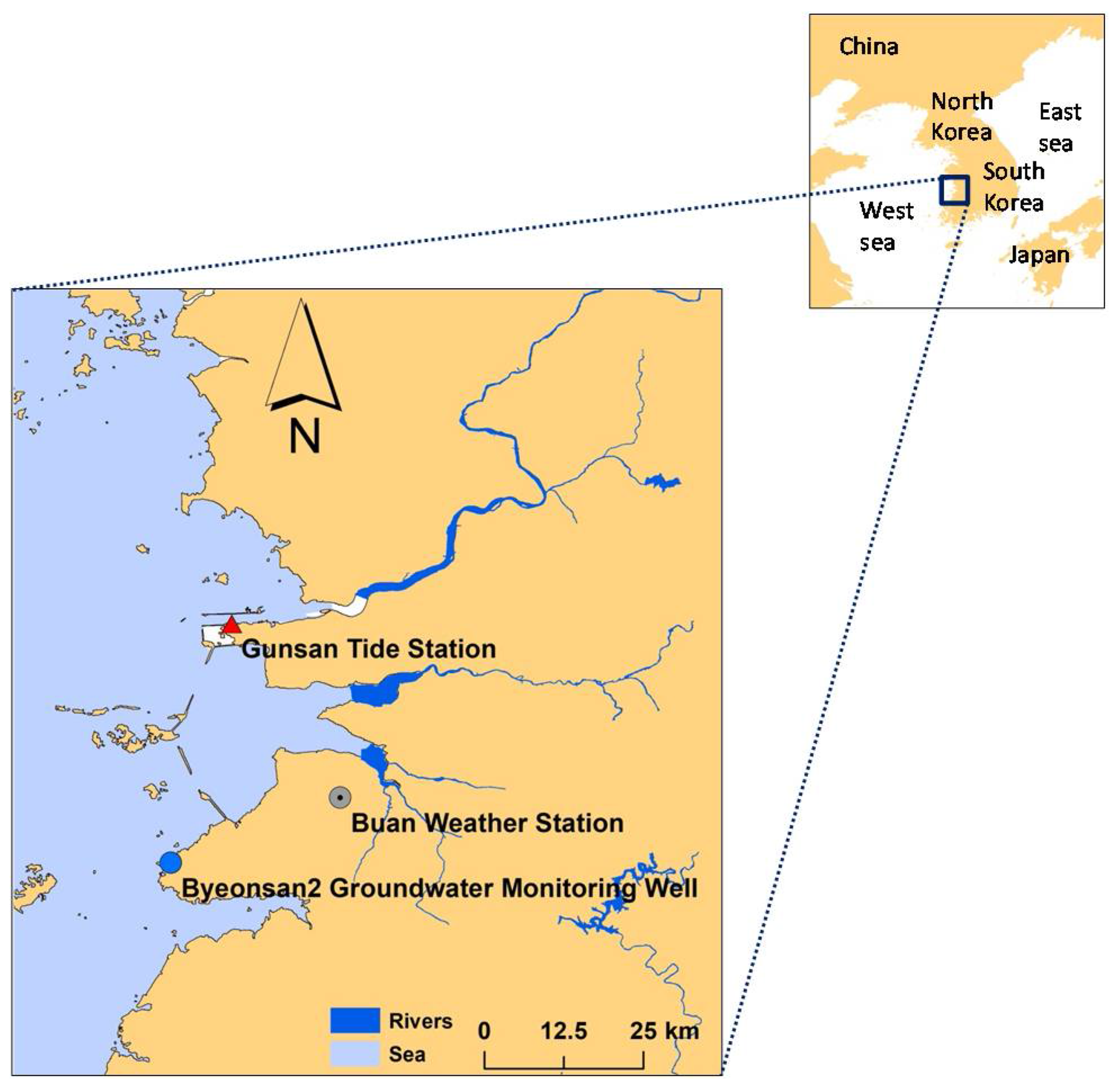
Figure 2.
The observed sea level data at the Gunsan tide gauge data: (a) hourly, daily, and monthly sea level data; (b) monthly seal level data; (c) seasonal cycle of sea level; and (d) monthly sea level data with no seasonal components. SSH is the sea surface height.
Figure 2.
The observed sea level data at the Gunsan tide gauge data: (a) hourly, daily, and monthly sea level data; (b) monthly seal level data; (c) seasonal cycle of sea level; and (d) monthly sea level data with no seasonal components. SSH is the sea surface height.
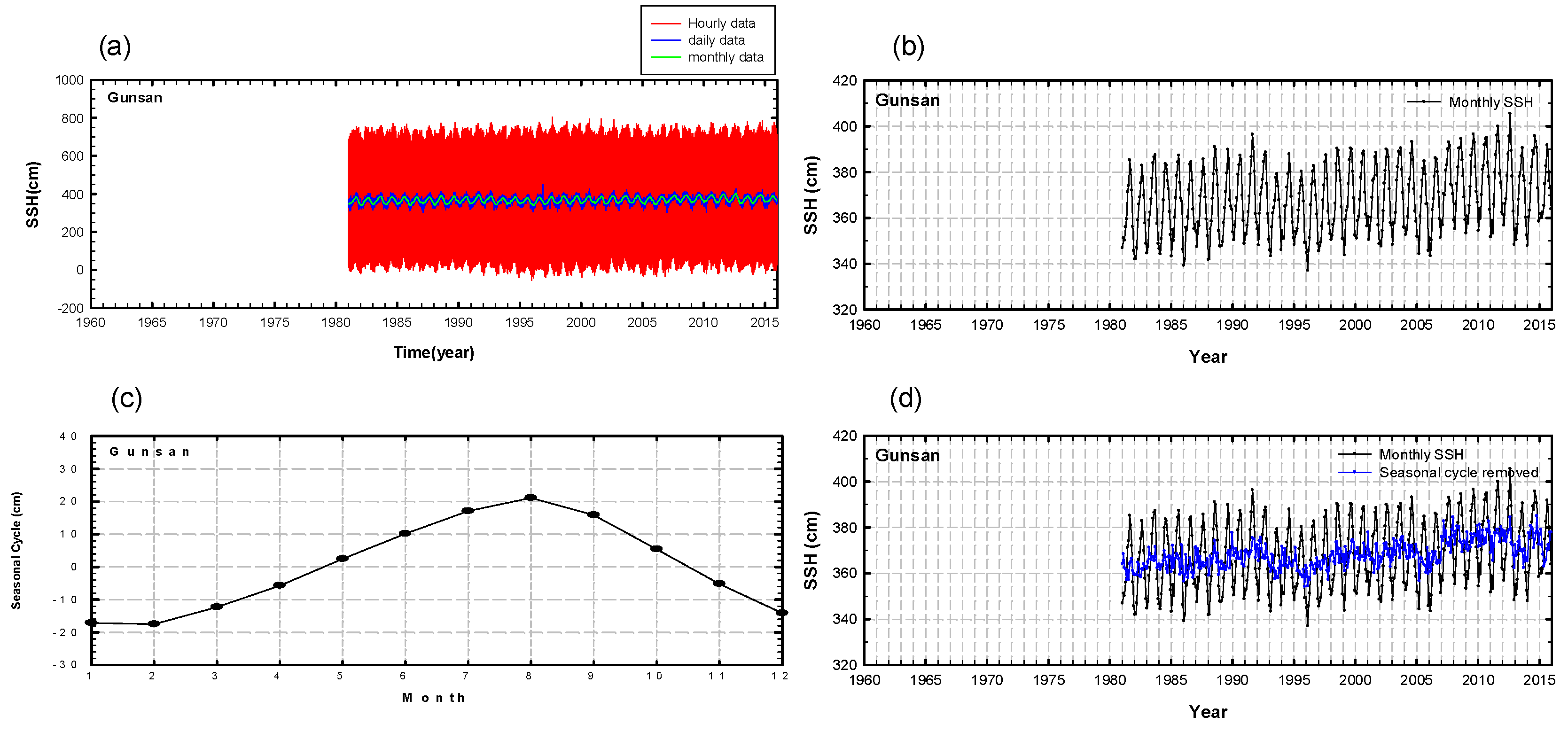
Figure 3.
Initial and boundary conditions and finite-element meshes for the simulation domain. ρsea = 1024.99 kg m−3; H = depth (m); g = 9.81 (m s−2); P = hydrostatic seawater pressure; Qin = freshwater recharge rate (kg m−2); Cin = 0.0 (kg kg−1); Csea = 0.0357 (kg kg−1). A total of 4637 nodes and 4539 elements were generated for the simulation domain.
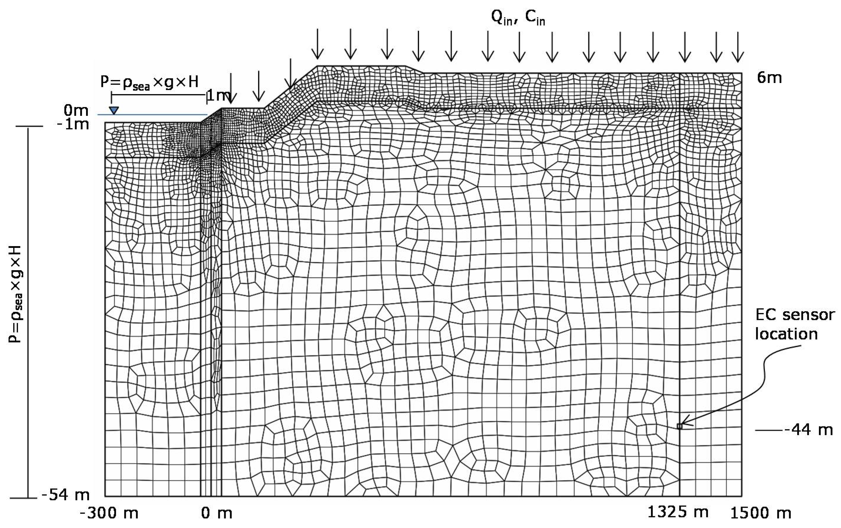
Figure 4.
Sea level (black curve), fitted straight line (blue line, linear trend), and fitted quadratic line (green curve, quadratic trend) at the Gusan tide gauge station.
Figure 4.
Sea level (black curve), fitted straight line (blue line, linear trend), and fitted quadratic line (green curve, quadratic trend) at the Gusan tide gauge station.
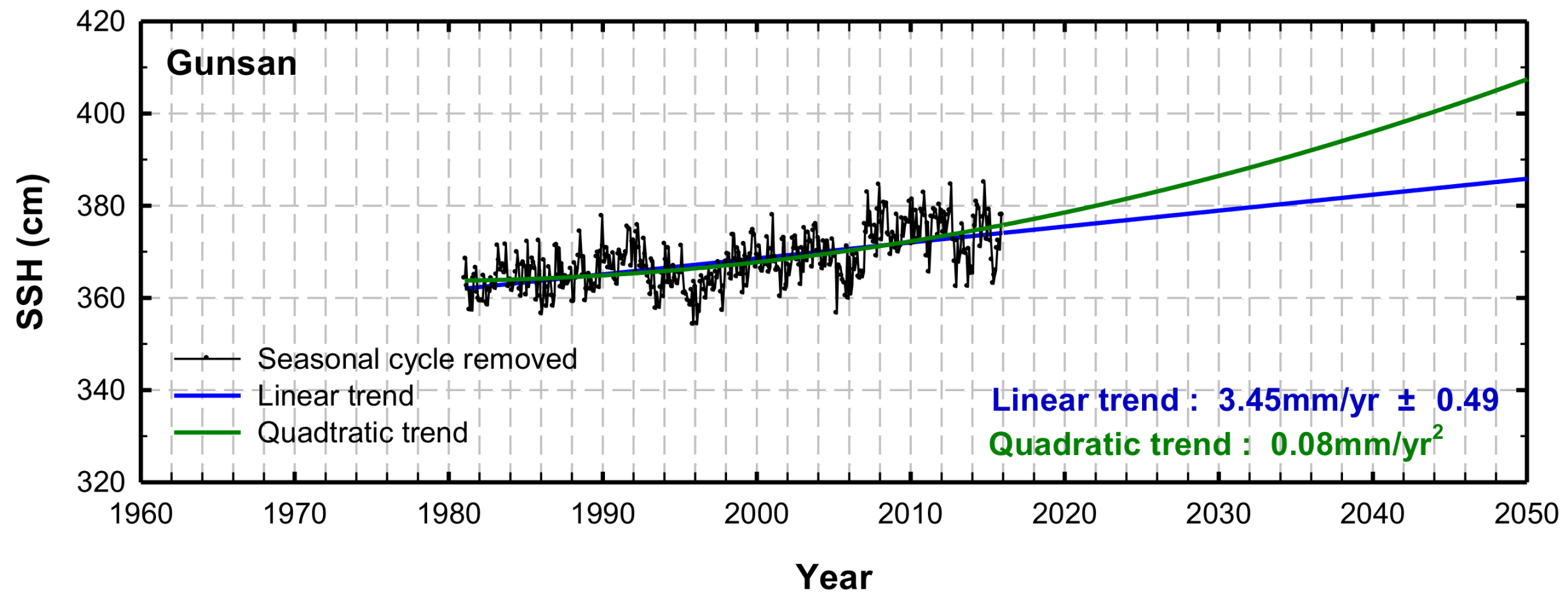
Figure 5.
Salinity changes (%) relative to the baseline at the observation node for the 14 scenarios.
Figure 5.
Salinity changes (%) relative to the baseline at the observation node for the 14 scenarios.
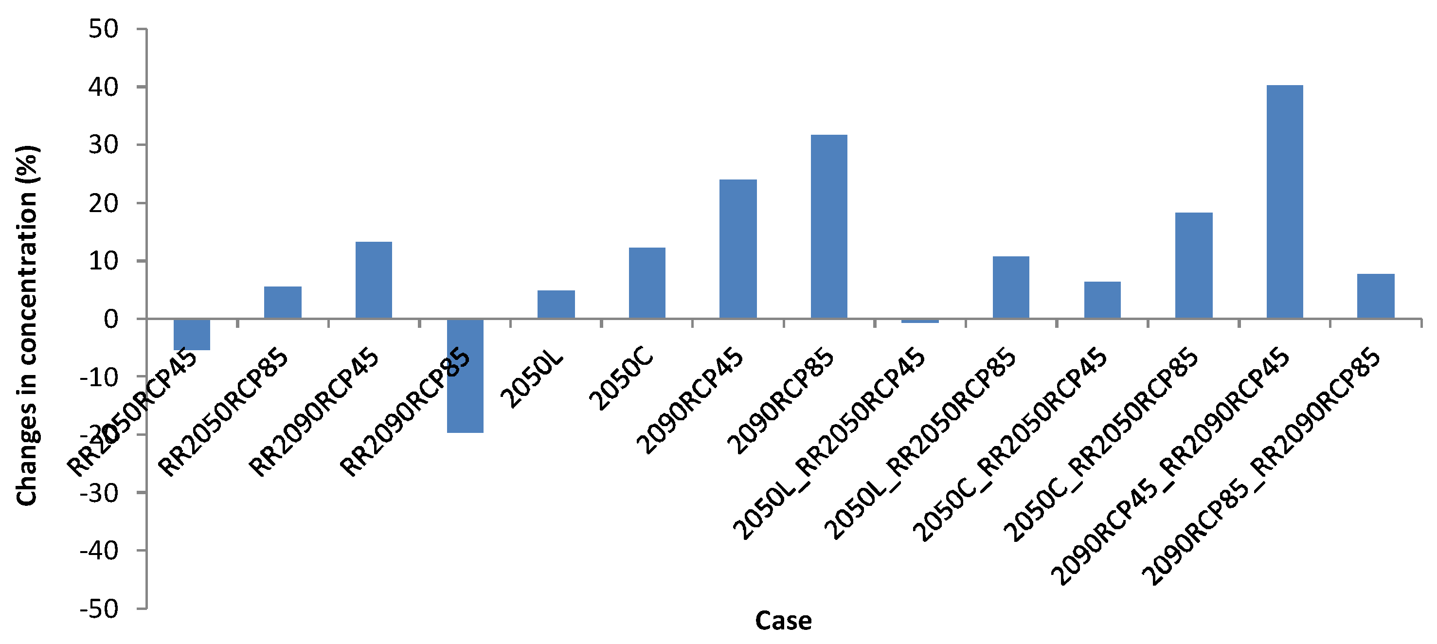
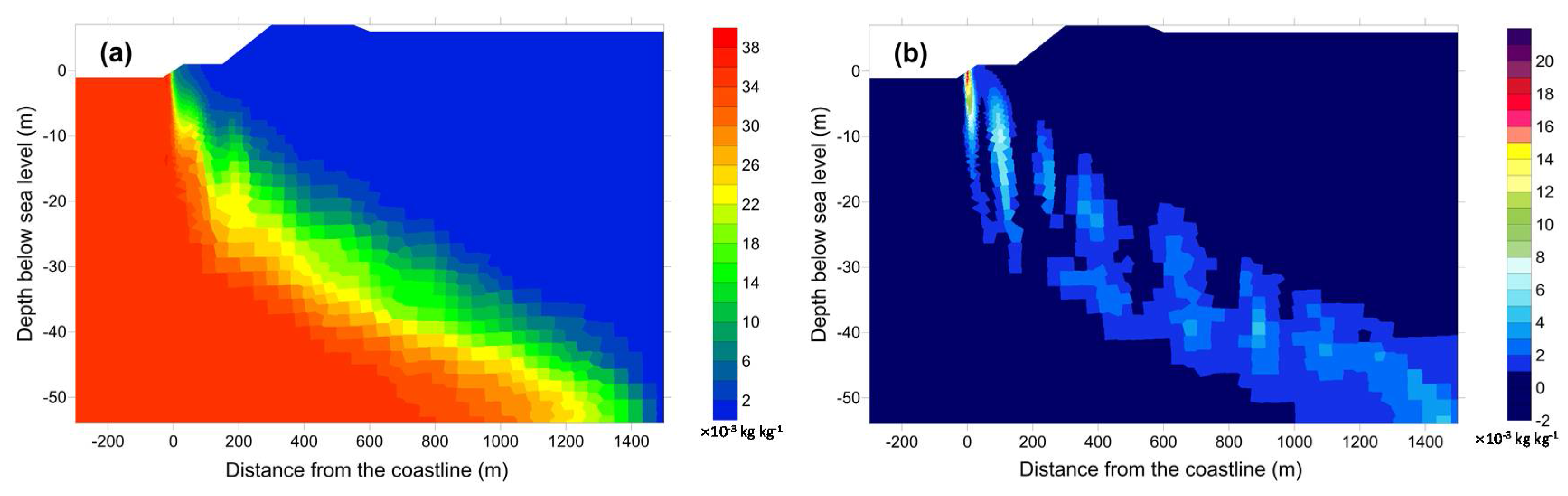
Figure 6.
(a) Salinity for the baseline and (b) salinity differences between the baseline and the scenario 2090RCP45_RR2090RCP45 2090RCP45_RR2090RCP45 (0.57 m SLR with a freshwater recharge rate of 0.0058 kg s−1) in × 10−3 (kg-dissolved solids) (kg-seawater)−1.
Figure 6.
(a) Salinity for the baseline and (b) salinity differences between the baseline and the scenario 2090RCP45_RR2090RCP45 2090RCP45_RR2090RCP45 (0.57 m SLR with a freshwater recharge rate of 0.0058 kg s−1) in × 10−3 (kg-dissolved solids) (kg-seawater)−1.


Table 1.
Fifteen scenarios, including the baseline with SLR and freshwater recharge rates.
| Cases | SLR (m) | Freshwater Recharge Rate (kg s−1) | Descriptions |
|---|---|---|---|
| Baseline | 0.0 | 0.00603 | 2005–2015 |
| RR2050RCP45 | 0.0 | 0.00627 | 2050s, RCP4.5, Precipitation (1) |
| RR2050RCP85 | 0.0 | 0.00580 | 2050s, RCP8.5, Precipitation (2) |
| RR2090RCP45 | 0.0 | 0.00549 | 2090s, RCP4.5, Precipitation (3) |
| RR2090RCP85 | 0.0 | 0.00694 | 2090s, RCP8.5, Precipitation (4) |
| 2050L | 0.12 | 0.00603 | Linear trend by 2050 (5) |
| 2050C | 0.32 | 0.00603 | Quadratic trend by 2050 (6) |
| 2090RCP45 | 0.57 | 0.00603 | SLR of the West sea under RCP4.5 (7) |
| 2090RCP85 | 0.72 | 0.00603 | SLR of the West sea under RCP8.5 (8) |
| 2050L_RR2050RCP45 | 0.12 | 0.00627 | (1) and (5) |
| 2050L_RR2050RCP85 | 0.12 | 0.00580 | (2) and (5) |
| 2050C_RR2050RCP45 | 0.32 | 0.00627 | (1) and (6) |
| 2050C_RR2050RCP85 | 0.32 | 0.00580 | (2) and (7) |
| 2090RCP45_RR2090RCP45 | 0.57 | 0.00549 | (3) and (7) |
| 2090RCP85_RR2090RCP85 | 0.72 | 0.00694 | (4) and (8) |
© 2018 by the authors. Licensee MDPI, Basel, Switzerland. This article is an open access article distributed under the terms and conditions of the Creative Commons Attribution (CC BY) license (http://creativecommons.org/licenses/by/4.0/).
Share and Cite
MDPI and ACS Style
Chun, J.A.; Lim, C.; Kim, D.; Kim, J.S. Assessing Impacts of Climate Change and Sea-Level Rise on Seawater Intrusion in a Coastal Aquifer. Water 2018, 10, 357. https://doi.org/10.3390/w10040357
AMA Style
Chun JA, Lim C, Kim D, Kim JS. Assessing Impacts of Climate Change and Sea-Level Rise on Seawater Intrusion in a Coastal Aquifer. Water. 2018; 10(4):357. https://doi.org/10.3390/w10040357
Chicago/Turabian StyleChun, Jong Ahn, Changmook Lim, Daeha Kim, and Jin Sung Kim. 2018. "Assessing Impacts of Climate Change and Sea-Level Rise on Seawater Intrusion in a Coastal Aquifer" Water 10, no. 4: 357. https://doi.org/10.3390/w10040357
Note that from the first issue of 2016, this journal uses article numbers instead of page numbers. See further details here.