Article

Model-Based Analysis of the Potential of Macroinvertebrates as Indicators for Microbial Pathogens in Rivers

by
Rubén Jerves-Cobo
1,2,3,*,
Gonzalo Córdova-Vela
4,
Xavier Iñiguez-Vela
4,
Catalina Díaz-Granda
5,
Wout Van Echelpoel
1,
Felipe Cisneros
3,
Ingmar Nopens
2 and
Peter L. M. Goethals
1
1
Laboratory of Environmental Toxicology and Aquatic Ecology, Department of Animal Sciences and Applied Ecology, Ghent University, Coupure Links 653, Ghent 9000, Belgium
2
BIOMATH, Department of Mathematical Modelling, Statistics and Bio-informatics, Ghent University, Coupure Links 653, 9000 Ghent, Belgium
3
Programa para el manejo del agua y del suelo – PROMAS, Universidad de Cuenca, Av. 12 de Abril s/n y Agustín Cueva, 010103 Cuenca, Ecuador
4
Asociación de Consultores Técnicos – ACOTECNIC Cia. Ltda., Aguaruna s/n y Autopista Cuenca Azogues, 010109 Cuenca, Ecuador
5
Empresa Pública Municipal de Telecomunicaciones, Agua Potable, Alcantarillado y Saneamiento–ETAPA EP. Ecuador, Benigno Malo No. 7–78 y Mariscal Sucre, 010101 Cuenca, Ecuador
*
Author to whom correspondence should be addressed.
Water 2018, 10(4), 375; https://doi.org/10.3390/w10040375
Submission received: 6 December 2017 / Revised: 16 March 2018 / Accepted: 21 March 2018 / Published: 24 March 2018

Abstract

:
The quality of water prior to its use for drinking, farming or recreational purposes must comply with several physicochemical and microbiological standards to safeguard society and the environment. In order to satisfy these standards, expensive analyses and highly trained personnel in laboratories are required. Whereas macroinvertebrates have been used as ecological indicators to review the health of aquatic ecosystems. In this research, the relationship between microbial pathogens and macrobenthic invertebrate taxa was examined in the Machangara River located in the southern Andes of Ecuador, in which 33 sites, according to their land use, were chosen to collect physicochemical, microbiological and biological parameters. Decision tree models (DTMs) were used to generate rules that link the presence and abundance of some benthic families to microbial pathogen standards. The aforementioned DTMs provide an indirect, approximate, and quick way of checking the fulfillment of Ecuadorian regulations for water use related to microbial pathogens. The models built and optimized with the WEKA package, were evaluated based on both statistical and ecological criteria to make them as clear and simple as possible. As a result, two different and reliable models were obtained, which could be used as proxy indicators in a preliminary assessment of pollution of microbial pathogens in rivers. The DTMs can be easily applied by staff with minimal training in the identification of the sensitive taxa selected by the models. The presence of selected macroinvertebrate taxa in conjunction with the decision trees can be used as a screening tool to evaluate sites that require additional follow up analyses to confirm whether microbial water quality standards are met.

1. Introduction

The most frequent health risk related to the ingestion of water is associated with microbial contamination by human or animal feces, which is a source of pathogenic bacteria, viruses, protozoa and helminthes [1,2]. Pathogens are introduced in rivers via point and non-point sources, and their autochthonous growth is stimulated by nutrients brought from the aforementioned sources [3]. The health risk increases when untreated wastewater from urban sewage systems (point source) is directly discharged into water bodies, potentially causing large outbreaks of waterborne diseases [4]. In addition, water from rivers and lakes has off stream uses such as drinking water or irrigation, and instream uses such as recreational activities with primary contact (e.g., swimming). Therefore, water quality control must always be of paramount importance [5].
The indicators often used to verify microbial contamination of water in developed countries are: total coliforms, and fecal coliforms and/or Escherichia coli [6,7]. Likewise, in many tropical countries, the assessment of running water quality is predominantly made by using physicochemical methods. However, most of the methods for determining physicochemical and microbiological parameters require expensive laboratory analyses that in the majority of developing countries, do not allow for the establishment of national rigorous monitoring programs of water bodies due to limited technical and financial resources. For those reasons, the development of cost-effective water monitoring programs is essential [8], and must include techniques for measuring microbial water quality.
The biological methods for monitoring river water health have evolved over more than a century. For example, benthic macroinvertebrates are used to assess the water quality over time, because they respond to both physicochemical changes and hydro-morphological variations within streams and rivers [9,10]. Physicochemical and microbiological parameters provide limited water quality information at a specific point in time [9,11]. In contrast, biological samples can also predict average values of chemical parameters when their cumulative effects have been more pronounced in the biota over a period of time preceding the biological sampling [11]. As such, the use of bioindicators in water quality assessment for streams has been integrated into the European Water Framework Directive [12]. In developing countries, biological river assessment was introduced and subsequently developed only recently [9], based mainly on adaptation of the English Biological Monitoring Working Party (BMWP) [13,14,15].
Fecal coliform (FC) concentration has been modeled using both deterministic and stochastic methods. The deterministic models focused on understanding the die-off variation of fecal coliforms in relation to temperature, and changes under kinetics conditions (i.e., transportation) such as the velocity along the rivers [16]. Alternatively, stochastic models have been used to obtain the relationship between fecal coliform and physicochemical [17] or microbiological [18] variables, or timing variation during a rainfall [19]. Negative correlation between FC concentrations and macroinvertebrate diversity (Shannon-Wiener diversity index) was observed in ponds [18].
On the other hand, the assessment of habitats and the determination of the relation between the presence of an organism and environmental variables has been done through the modeling of running waters based on ecological, physicochemical and microbiological parameters. These modeling techniques have allowed for the handling of the non-linear behavior of the ecosystem, obtaining models with a high reliability [20,21,22]. In this way, the FC has been associated as one of the explanatory variables describing the presence or absence of some taxa of macroinvertebrates [22,23,24]. Machine learning with different modeling techniques, such as classification trees (CTs) combine reliable classification predictions with transparency, and have been proven to be effective to assess running waters [25,26]. The CTs provide good modeling techniques as they focus on the presence/absence or abundance of macroinvertebrate taxa (family or species) in relation to a specific impact or a disturbance in the streams [11,20,26,27,28]. Consequently, considering the described correlations between fecal coliform presence and macroinvertebrate diversity [18,22,23,24], compliance to regulatory standards can be simulated based on the prevailing macroinvertebrate community structure by training classification trees on combined observations of fecal coliforms and macroinvertebrates, thereby acting as a proxy indicator for fecal coliform contamination.
In our research, with the environmental and biological variables collected in the Machangara River in Ecuador between February and March of 2012, three decision tree models (DTMs) were developed as indicator tools to check the compliance to three of the Ecuadorian microbial water quality standards associated with fecal coliforms. The construction of the DTMs was based on the presence and abundance of macroinvertebrates in the Machangara River basin. The models were built based on statistical adjustments and ecological criteria. For model optimization, statistical techniques were used, such as the elimination of false positives (FP) achieved by applying weights as well as the minimum confusion entropy from the models. Two of the three final obtained DTMs were validated with datasets collected in July of 2015 and March of 2016.

2. Materials and Methods
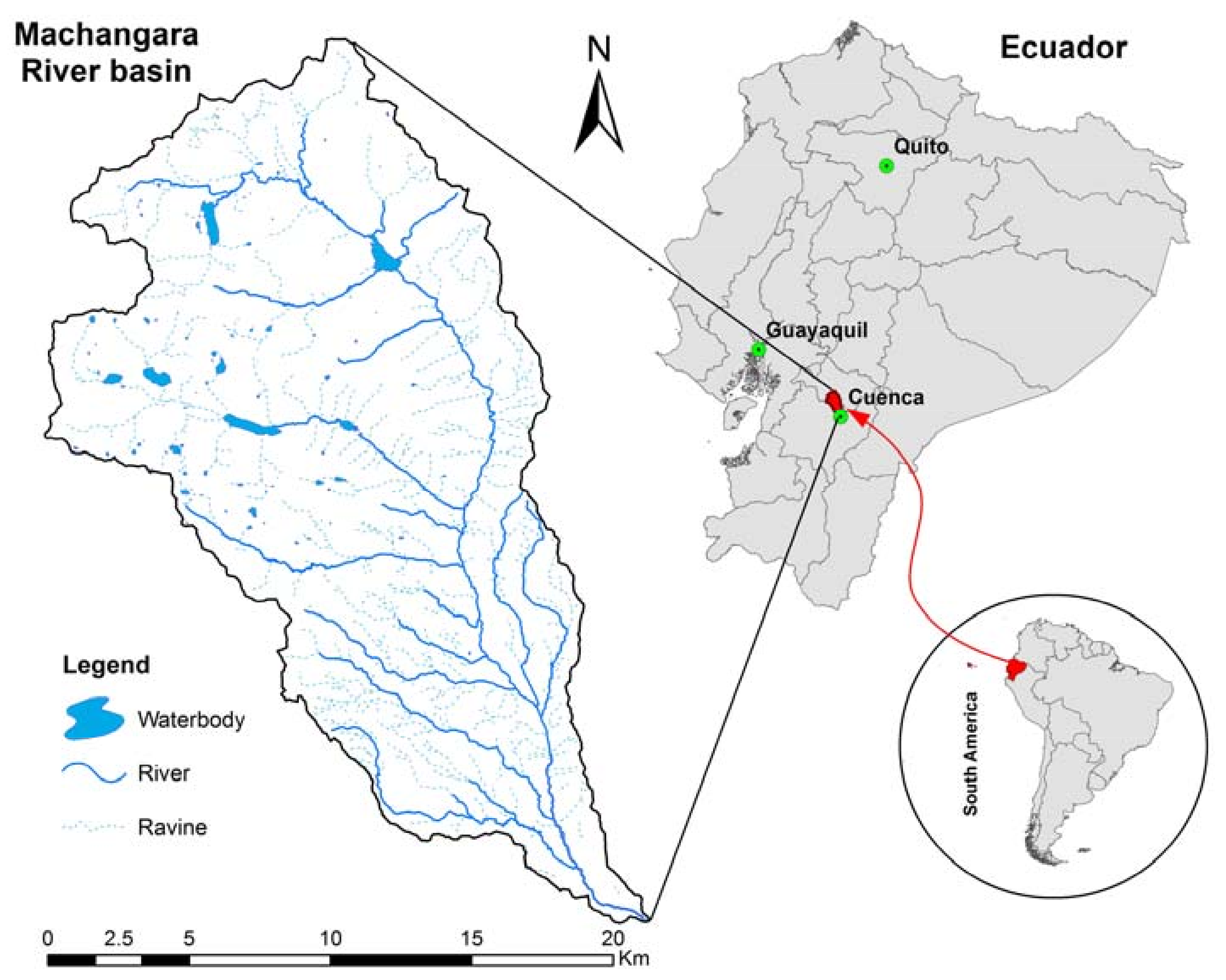
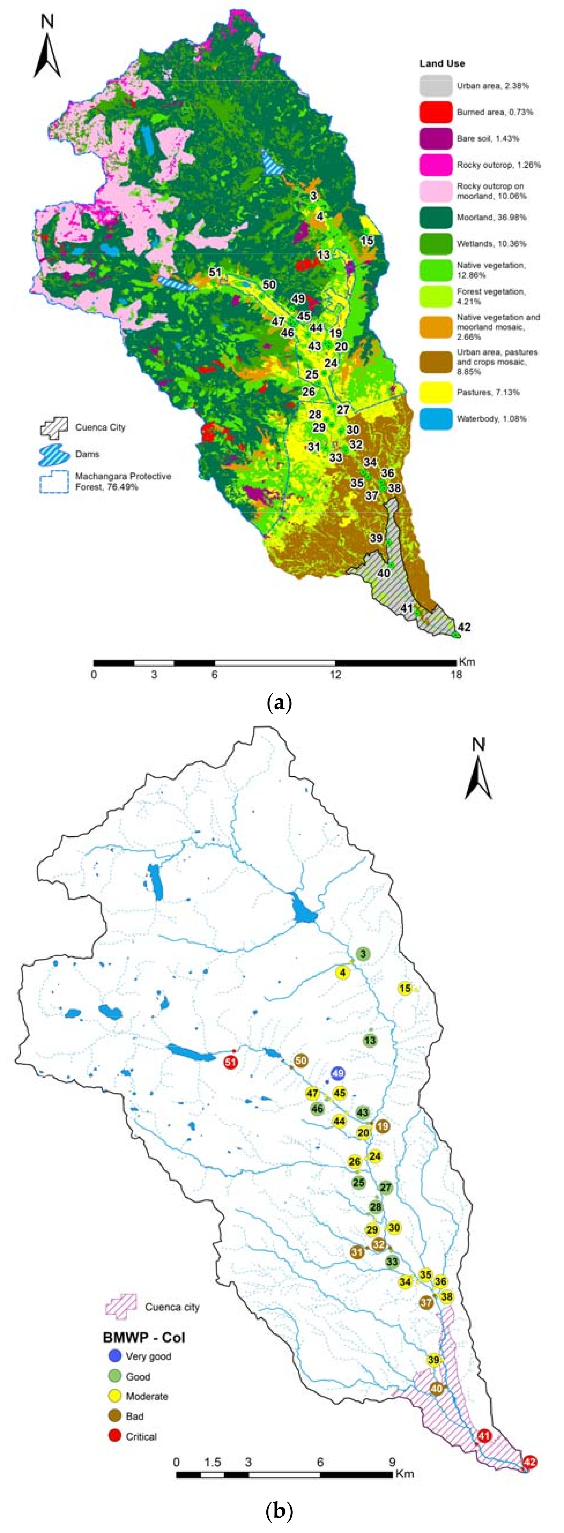
2.1. Study Area

This study focuses on the basin of the Machangara River, which is an Andean mountain river that in its origin is a river of the first order, finishing as a river of the fourth order upon its discharge into the Cuenca River. The Machangara River is about 37 km in length [29], and at the end of its path, crosses the city of Cuenca, located in the southern Province of Azuay in Ecuador (Figure 1). Cuenca is the third largest city in the country with an estimated 2015 population of about 370,000 inhabitants [30]. The Cuenca River basin is part of the Hydrographic Demarcation Santiago, one of the Amazon Effluents.
The Machangara River is about 325 km2, of which 252 km2 is forest protected by the Ecuadorian government. The aforementioned basin is regulated all year by two hydroelectric power plants, with their respective dams, Labrado and Chanlud, situated in the upper area of the catchment and upstream from Cuenca (Figure 2a). Water is extracted from the catchment basin for use primarily as a supply of drinking water, agricultural irrigation, and to a lesser extent for industrial use. The altitude of the basin varies from 2440 to 4420 m above sea level (m a.s.l.) and its mean altitude is 3557 m a.s.l. The average annual rainfall in the basin varies from 877 mm in the lower part to 1363 mm per year in the upper areas. With regard to the average annual temperature, this fluctuates between 16.3 °C in the lowlands to 9.0 °C in the more elevated areas of the Machangara basin [31,32]. Two seasons, which are distributed in two periods each, are present during the year: the rainy season from the middle of February until the beginning of July, and from the second half of September until the first two weeks of November with the dry season being the rest of the year. The monthly average discharge of the Machangara River from 1964 to 2010 at its outlet the Cuenca River was 8.4 m3·s−1, the average minimum monthly discharge was 5.3 m3·s−1 in August and the average maximum monthly discharge was 14.6 m3·s−1 in May [33].
Despite the combined sewage system in Cuenca, poor water quality results occurred along the parts where the river flows through the city. This is mainly due to some sewage networks and industrial pollution points that are discharging in different locations along the river and its tributaries that are affecting the water quality of these streams [29,34]. In addition, discharges from combined sewer overflow (CSO) events, when wet-weather flows exceed the sewage treatment plant capacity, and surface water outfalls (SWO) cause the degradation of physicochemical and biological quality [35,36,37,38]. Similarly, pollution from agricultural and livestock runoffs transport polluted water into the rivers [39]. This poor water quality in the river running along the city, could have been influenced by pollutants such as organics expressed as BOD5, organic nitrogen, phosphates and fecal coliforms [29].

2.2. Data Collection

The dataset used in this research was collected and measured once during the rainy season in February and March 2012, while the validation datasets were sampled in the last half of July 2015 in dry season and in March of 2016 in rainy season. The dataset used for the model development considered 33 sampling locations measured in 2012, which were chosen along the catchment according to land use (Figure 2a and Figure S1 in Supplementary Materials). In the validation datasets, the samples were collected from 14 points in July of 2015 and from 11 sites in March of 2016 (Figure S1 in Supplementary Materials). In each point sampled in 2012, 17 physicochemical, hydraulic, microbiological, and biological variables were measured (Table A1 in the Appendix A). From this data, four variables were measured in situ: water temperature, conductivity, dissolved oxygen (DO) and pH with an ORION 5Star 1219001 (Thermo Scientific, Waltham, MA, USA) multi-parameter probe. Flow velocity was measured using the float method described by the U.S. Environmental Protection Agency [40]. The rest of the parameters and the methods used by their determination in the laboratory of Sanitation at the Water Supply and Wastewater Management Municipal Company ETAPA—EP in Ecuador, are shown in Table A1 (Appendix A).
Benthic macroinvertebrates samples were collected from the rivers and their tributaries by using the kick-sweep method. This method is applied by shuffling the feet walking backwards against a current while holding a standard net (inlet area 575 cm2, mesh size 500 μm, depth 27.5 cm) for six minutes in a stretch of approximately 10–20 m, allowing personnel to collect in the net the material from immediately upstream. One kick net sample was collected in each site, which included all different habitats present such as bed substrate, litters, macrophytes and parts of terrestrial vegetation immersed in the water. Additionally, macroinvertebrates were manually picked from stones and leaves [41,42,43]. Macroinvertebrates were then sorted in the field and preserved in ethyl alcohol at 70% [43]. All macroinvertebrates collected were identified in the laboratory to family level with the help of a stereoscope, with magnifications that varied from 0.8× to 5×, and specific reference materials [44,45,46]. At each sampling location, the Biological Monitoring Working Party index adapted to Colombia (BMWP-Col) [15,45,47], was calculated (Figure 2b), which takes into account the score of sensitivity to organic pollution of the taxa found. The range of the sensitive score goes from one (for very tolerant taxa), to 10 (for most sensitive families). BMWP-Col is calculated as the sum of the sensitivity scores of each taxa captured in each site. BMWP-COL scores can be divided into five water quality categories that consist of: bad (≤15), deficient (16–35), moderate (36–60), good (61–99) and very good (>99) [45,47].

2.3. Ecuadorian Water Regulation in Relation to Water Use

The Ecuadorian government has regulations regarding the water quality in relation to water use [48]. The standard norm set a value limit for different parameters in relation to particular water usage, giving three thresholds to regulate the concentration of fecal coliforms with regard to water use (Table 1). The most stringent microbial water quality standard for fecal coliforms is applied for recreational water use with primary contact (Table 1). The least stringent microbial water quality standard for fecal coliforms is for raw (untreated) water used for drinking water before receiving non-conventional treatment (Table 1). Non-conventional treatment methods include slow sand filtration and multi-stage filtration, which is recommended for small towns that need flows less than 8 L/s and a population <5000 people whose town needs flows up to 21 L/s and a population <12,000 people [49]. The intermediate microbial water quality standard for fecal coliforms is for agriculture (Table 1).

2.4. Model Development

Decision tree models (DTMs) were developed to predict the fecal coliforms regulation fulfillment according to the water uses (Table 1), and were expressed as three discrete levels. In this research, the attributes or independent variables of the DTMs were the presence/absence or abundance of macroinvertebrates taxa that were observed in at least three sampled points (Table 2). The discrete dependent variables were in fulfillment of the three microbial water quality standards for fecal coliforms, which were measured as most probable number per 100 mL (MPN.100 mL−1). The decision trees are hierarchical structures, where internal nodes contain a test on the input independent variables. Each branch of an internal test corresponds to an outcome of the test and the prediction for the values of the dependent variable is stored in a leaf. Each leaf of the decision tree contains a prediction for the dependent variable. Decision trees explain variation in dependent variables by splitting independent variables at certain thresholds in the node of the tree. Furthermore, each division or level can produce more nodes with branches that follow a new ordering instruction [50,51,52,53]. Decision trees have been applied in numerous ecological studies such as macroinvertebrate habitat suitability analysis [20,27], because the DTM combines reliable classification with a transparent set of rules [52]. Furthermore, the classification trees are robust techniques that can deal with small datasets [54] less than 50 data points [55], particular to the case of this study, in which the dataset is composed of the results of 33 different sites. In addition, with a small dataset the accuracy of the classification trees models is higher than other techniques such as logistic regression models [56]. All observations were included to construct the models, because classification trees are not sensitive to outliers [57].
In this study, the machine learning software, Waikato Environment for Knowledge Analysis (Weka) [58], and its package J4.8 decision tree classifier that is a Java re-implementation of C4.5 [59] were used for inducing classification trees and creating a prediction model. The model training and validation were performed with three, five, ten-fold (k-fold) cross validation (three, five, 10, k fcv) in which the records are randomly split into k equally-sized subsets. In each set, k-1 subgroups are used as the training set and the k-th that remains is run as the test set. This process is repeated k times and each subset is used as the test set exactly once [28]. The expansion of the tree is stopped with the pruning process, which gives to every leaf, a minimum number of instances to allow branching. With the aim to improve this process, two pruning confidence factors (PCF) were employed: 0.25, which is the default value, and 0.1. With a small dataset, lower cross validation values can result in more robust models, but with a relatively low performance [60]. Table 3 and Table A2 in Appendix A show the settings for the eight models obtained with three, five, 10 fcv and 66% of data as a trained set, as well as a PCF of 0.1 and 0.25, before optimization.

2.5. Model Optimization

Optimization was achieved by adding costs with a cost-sensitive classifier (CSC) tool with the J4.8 algorithm in the WEKA software. The CSC process gives new weights in training instances according to the total cost assigned to two kinds of errors: false positives (FP), which are known as type II errors, and false negatives (FN), which are identified as type I errors, with the least expected misclassification cost rather than the most likely one [58]. An FP occurs when the result is incorrectly predicted as fulfillment, while an FN happens when the outcome is incorrectly predicted as non-fulfillment [27,61]. The differences between the cost sensitive classifier (CSC) with the J4.8 algorithm is the initial setting in this process in which different weights to false positive have been given in the cost matrix that seeks to minimize the number of type II (i.e., FP) errors, and the total misclassifications cost calculated in the confusion matrix [62,63]. As an effect of the initial weight setting in the cost matrix, where the false positives (FPs) have been weighted higher than the false negatives (FNs), the confusion matrix will have fewer FPs than FNs [58]. All the setting values used to construct 40 models, when the cost matrix optimization was applied, are displayed in Appendix A (Table A2), while the settings of the models with the greatest accuracy are shown in Table 4.

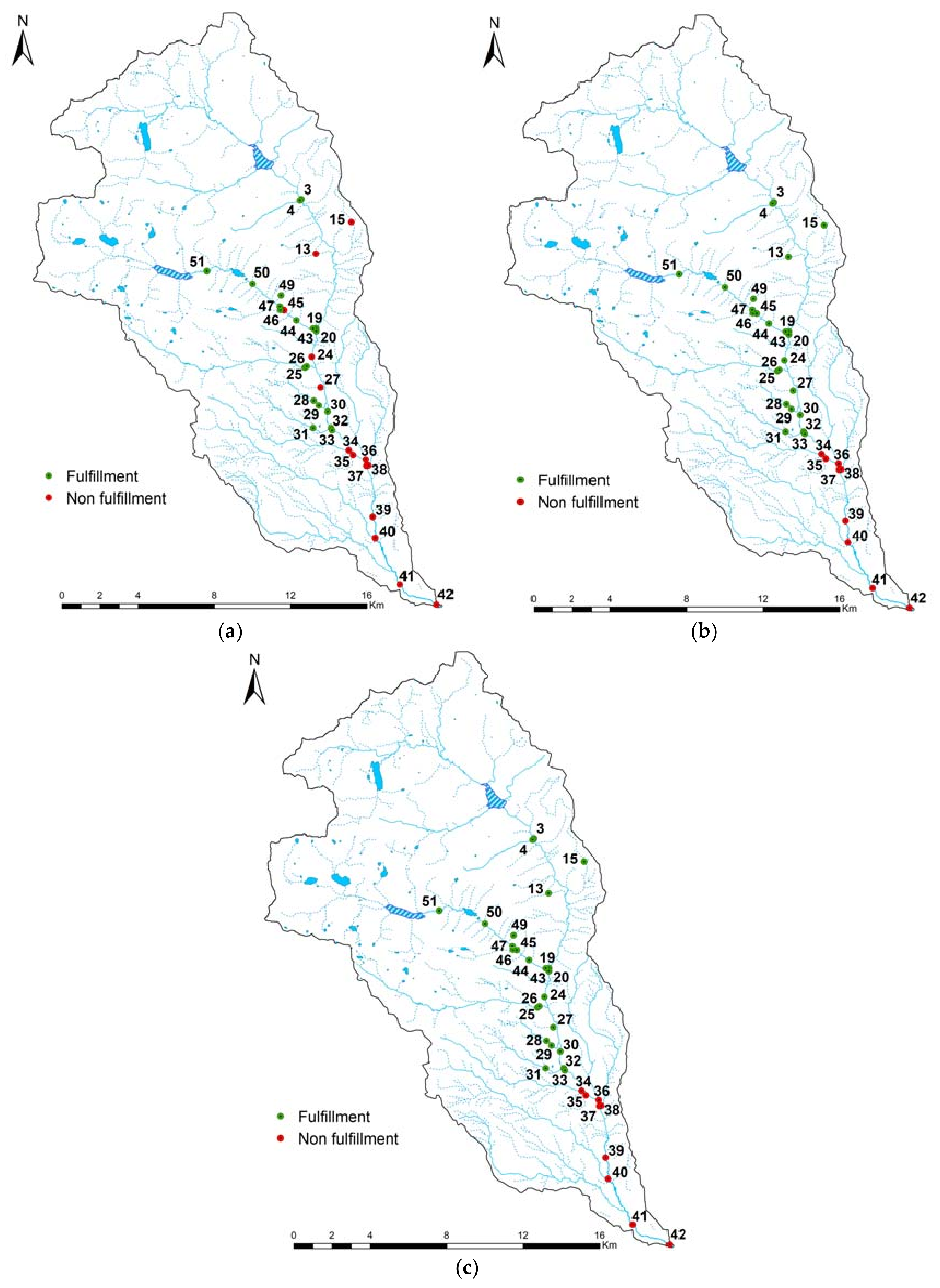
2.6. Modeling and Analysis

First, the accuracy of the DTMs was evaluated with two measurements obtained from the confusion matrix. This matrix identifies true positive (TP), false positive (FP), false negative (FN) and true negative (TN) cases predicted by each run.
The first fitted measure was the number of correctly classified instances (CCI), which is calculated as the sum of the diagonal (i.e., TP + TN) divided by the sum of all values (i.e., TP + FP + TN + FN) [64]; a value expressed in percentage. The CCI range is from 0 to 100%, where a value of 100% has the greatest accuracy of the model [65]. The second fitted ratio was Cohen’s Kappa statistic, which is a derived statistic that measures the proportion of possible cases of correct predictions (TP and TN) by a model after accounting for chance predictions [27,66]. This coefficient is calculated as:
K a p p a = ( T P + T N ) ( T P + F N ) ( T P + F P ) + ( F P + T N ) ( F N + T N ) n n ( T P + F N ) ( T P + F P ) + ( F P + T N ) ( F N + T N ) n
The interpretation of the model fit with respect to different Kappa statistic values is as follows: Poor (<0), Slight (0–0.20), Fair (0.21–0.40), Moderate (0.41–0.60), Substantial (0.61–0.80) and Almost Perfect (0.81–1.0) [67]. Models are considered good when the Kappa statistics is higher than 0.4 and CCI at least 70% [28].
When the cross validation results, which are calculated beginning with the confusion matrix, are slightly different, it is difficult to determine in the first instance which measurement is better for evaluating a decision tree model (DTM). Furthermore, the accuracy of the DTM (i.e., CCI) is uniquely obtained regardless of how the other off-diagonal elements take their values [68]. The misclassification information (i.e., FP + FN) of confusion matrices can be analyzed using the measurement of the overall confusion entropy of a confusion matrix (CEN), which evaluates the confusion level of the class distribution of misclassified samples. According to Wei, Yuan, Hu and Wang [68], higher accuracy of the models is likely to correspond to lower confusion entropy. Likewise, the CEN is more precise than the correctly classified instances (CCI), and can replace this latter coefficient to evaluate classifiers in classification applications. In addition to the CCI, the least confusion entropy was considered as a decision value to choose the best model for each analyzed regulation. For this calculation, the following expression was adapted to a confusion matrix of 2 × 2, from equations given by Wei, Yuan, Hu and Wang [68]:
C E N = ( P 1 + P 2 ) C E N j
where, P j is called confusion probability of class j and C E N j is defined as confusion entropy of class j . These values were calculated with the next expressions Equations (3) and (4).
P 1 = T P + F N 2 ( T P + F N + F P + T N )   a n d   P 2 = F P + T N 2 ( T P + F N + F P + T N )
C E N j = P F N l o g 2 P F N P F P l o g 2 P F P
In Equation (4) P F P and P F N are the misclassification probability of classifying the samples of class i to class j subject to class j , are defined in Equation (5).
P F P = F P F N + F P + 2 T P   a n d   P F N = F N F N + F P + 2 T N
In order to check the stability of the DTMs, and knowing that the dataset is relatively small, the dataset was randomly and manually divided into three subsets, and stratified based on fulfillment or non-fulfillment of the regulation in analysis. Two of these subsets were used to train the model, and the third subset was applied to test the model. This process was repeated three times so that each subset was used to check the others. Furthermore, the groups of two subsets used for the learning process were settled on J4.8 with a pruning confidence factor of 0.25 and 0.10. Additionally, when a false positive (FP) was detected in the confusion matrix, the cost-sensitive classifier (CSC) tool was employed to give new weights to the FP. The Stability of the DTMs was calculated from the wide variation of the standard deviation [28] of the CCI and Kappa statistics [54] that were obtained from the test subsets.
The optimization of the models to be used for more than statistical fit perspective must be assessed from an ecological point of view. In some cases, erroneous results from an ecological angle could also occur. For this reason, before choosing a model, an ecological examination has to be considered [69], in which the obtained rules from the DTM are compared and tested for what is generally accepted in ecology [70]. Thus, for example, an acceptable knowledge rule is: “The ecosystem has a higher ecological status when the concentration of nutrients is low”. While, an erroneous knowledge is for example: “The quality of the ecosystem is very high with a low oxygen concentration” [69]. Thus, in this research for the ecological evaluation, two criteria were included. The first, the DTM, was discarded when a taxon resulting from the model had a tolerant score (TS) lower than four, which ensured that the microbial water quality assessment was not done in a highly polluted place. The second criterion was to ensure that at least one of the taxon resulting from the DTM was always present. In some cases, it is possible to obtain from the branches (rules) of a DTM that the presence of any taxon is not necessary for compliance with the fecal coliform regulation. This is an aspect that could give erroneous results on the application of the DTM.
Finally, the selected models, after optimization process were assessed with two new datasets taken both in dry (July of 2015) as well as in rainy (March of 2016) seasons.

3. Results

3.1. Current Water Quality Status

Fecal coliforms concentrations were greater in urban and suburban sites than sites from other land uses (Figure 3), while a summary of the variation of the physicochemical parameters collected during the sampling campaign can be reviewed in Table A1.
Similarly, the fecal coliforms results, in relation to the three microbial water quality standards described in Section 2.3 and with land use (Figure 2a, Table 2), show that the nine points sampled in the south–east section of the basin that are located in the urban and suburban areas of Cuenca, do not meet the official microbial water quality standards (Figure 4a–c). All other locations (24 points) meet the regulation standards regarding agriculture (<1000 MPN.100 mL−1) and raw water (<2000 MPN.100 mL−1). It is important to note that these 24 sites met both regulations at the same time. Additionally, nine points previously indicated, five sites are not meeting the recreational regulation (<200 MPN.100 mL−1). The location of the aforementioned five sites is close to livestock zones: three are near the center of the Machangara basin (points: 24, 27 and 45), and two other locations are in the northeast area of this catchment (points: 13 and 15) (Figure 4a).
In total, 36 taxa of macroinvertebrates were captured (Table 2), which were the basis for the calculation of the BMWP-Col. When analyzing the results of the BMWP-Col of the 33 points indicated in Figure 2b, in relation to the fecal coliforms regulations, the outcomes show 14 points with different biological water quality (i.e., two good, eight moderate, two deficient, and two bad) that do not meet the recreational fecal regulation. In addition, nine points with diverse BMWP-Col (i.e., five moderate, two deficient and two bad), do not meet the values of the agriculture and raw water fecal regulations.

3.2. Model Development

For the construction of the models, 23 taxa that were observed in at least three different points were used (Table 2). In total eight models were constructed during the model development stage, from which four resulted from the absence-presence dataset while that four other models developed with the abundance dataset (Table 3 and Table A3 in Appendix A). Based on the correctly classified instances (CCI) and Kappa statistics, a reliable decision tree model (DTM) (i.e., CCI > 70% and k > 0.4) obtained from models 2a1 and 2a2 (Table 2), was developed with the abundance database, allowing a preliminary assessment of the fulfillment of the agriculture fecal coliform guidelines (Figure 5b). No reliable model was obtained to assess the fulfillment of the recreational fecal coliform regulation. Similarly, from the presence-absence database no confident DTMs (Table 3) were obtained to check the accomplishment of any fecal coliforms guidelines. With the dataset used, it was not possible to obtain a specific model to verify raw water regulation, although the model obtained for agriculture fecal regulation, which has a more stringent threshold, could be adopted to check the raw water regulation. Likewise, the two best models had as a result, the same DTM (Models 2a1 and 2a2—Table 3), whose description is shown in Section 3.3 following an ecological examination.

3.3. Model Optimization

The decision tree models (DTMs) were optimized adding new weights to false positives in training instances, with the aim to minimize the false positive (FP) errors. This is possible with a cost-sensitive classifier (CSC) tool with the J.48 algorithm in the WEKA package. It was not possible to obtain a specific model for the raw water fecal regulation, but the resulting DTMs obtained from the agriculture regulation could be applied to check the raw water fecal regulation. Moreover, the threshold of the agriculture regulation is more stringent than the raw water fecal coliform regulation. In this stage 40 models were developed (Table A4 in Appendix A), from which eight DTMs were reliable (Table 4), with their correctly classified instances (CCI) higher than 0.7 and with their Kappa statistics higher than 0.4 (Table 4). These eight DTMs were initially pre-selected from a statistical point of view (Table 4). Two groups of models for evaluation of the recreational fecal coliform regulation had similar trees with different abundance requirement (models from 1a5 to 1a7 and from 1a9 to 1a12), that group which had the model with the least entropy of a confusion matrix (CEN) was chosen (models from 1a5 to 1a7). For the agriculture fecal regulation, the DTM resulting from models 2a3 to 2a6 was the same that was obtained in models 2a1 and 2a2 in the previous section, “Model development”. The DTMs achieved from models 2a3 to 2a6 and from 2a7 to 2a11 had the same families with the same requirements of abundance, differing between both DTMs the sequence of their leaves. In this case, the group that had the model with the least CEN was selected (models from 2a3 to 2a6), resulting in six total DTMs after statistical evaluation (1a4, 1a5 to 1a7, 1a8, 2ap3, 2ap4 and 2ap5, and 2a3 to 2a6—Table 4). All models that were obtained after the optimization process with their results of the correctly classified instances (CCI), Kappa statistics, the number of leaves obtained in each model through k-fold (i.e., three, five and 10) cross validation and the overall confusion entropy of a confusion matrix (CEN), are shown in Table A3.
These pre-selected decision tree models (DTMs) were verified from an ecological point of view. Three group of models were discarded: the first with the model 1a4, the second with the model 2ap3, and the third with the models 2ap4 and 2ap5 (Table 4 and Table A4 in Appendix A). Chironomidae, which is a taxon with very low pollution sensitivity, is present in the leaves of the first discarded 1a4 DTM (Table 4). This 1a4 model was constructed with the abundance dataset to assess the fulfillment of the recreational fecal coliform regulation, while, the second (model 2ap3) and third (models 2ap4 and 2ap5) DTMs were developed with the absence-presence dataset, to evaluate the accomplishment of the agriculture fecal coliform regulation. In those DTMs, the rules are determined by the presence and absence of Perlidae and Baetidae taxa. The absence of both aforementioned sensitive taxa meets the agriculture fecal coliform regulations (Tables S2 and S4—Supplementary Materials). However, this situation can also register in polluted sites.
The three remaining DTMs (1a5 to 1a7, 1a8 and 2a3 to 2a6—Table 4) were evaluated with the validation datasets, from which two models were confirmed (1a5 to 1a7 and 2a3 to 2a6—Table 4), whereas the one DTM obtained from model 1a8 (Table 4), constructed for verification of recreational water use with primary contact guidance, could not be validated nor discarded. Validation was not possible due to the fact that the latter DTM did not meet with the requirement of abundance given by its second branch (Table S3 in Supplementary materials). This, despite the fact that the first branch of the model met the FC regulation and was validated.
Finally, two decision tree models (DTMs) were selected (from models 1a5 to 1a7 and from models 2a3 to 2a6—Table 4), in which the abundance of each taxon refers to the number of specimens collected in five square meters (5 m2). The first DTMs is applicable as preliminary tools for verification of recreational water use with primary contact guidance, which is referred to in this work as the ‘recreational fecal regulation’. This first DTM (from models 1a5 to 1a7—Table 4) has as a condition, the presence of Baetidae (Ephemeroptera) with an abundance less or equal to three and the presence of Scirtidae (Coleoptera) with an abundance minor or equal to three (Figure 5a). The second DTM (from models 2a3 to 2a6—Table 4) is used as a proxy indicator to evaluate the success of the agriculture fecal standards that regulate agriculture and livestock water uses. This second DTM (from models 2a3 to 2a6—Table 4Figure 5b) was the same that was obtained before the optimization step (models 2a1 and 2a2—Table 3). The model showed that the presence of Perlidae (Plecoptera) is necessary, if this taxon is not present, Baetidae (Ephemeroptera) must have an abundance of one but less than or equal to four. If its abundance is higher, the non-fulfillment of the regulation is complete. The rules generated by the leaves of the chosen DTMs were also checked with the fulfillment of the recreational and agriculture fecal coliforms regulations (Tables S1 and S2—Supplementary Materials), as well as the validation datasets (Tables S3 and S4—Supplementary Materials), verifying that all points that met the requirements of the DTMs satisfied the analyzed fecal coliforms standards.
The stability of the models of the same class (e.g., 3-fcv and 0.10 as PCF) was determined by the variation among correctly classified instances (CCI) and Kappa statistics obtained from the tree fold cross validation. The results shown in Supplementary Materials (Tables S5 and S6), demonstrate that on average the standard deviation represents 20% of the mean of the CCI and 61% of the mean of the Cohen’s Kappa statistics, for the models of the recreational fecal regulation. While, for the agriculture regulation models, the standard deviation is, on average 14% of the CCI and 73 % of the Kappa statistics. This revealed that the CCI deviation was acceptable, while for the Kappa statistics the variation range was high.

4. Discussion

4.1. Model Relevance and Optimization from a Statistical Point of View

Classification trees successfully modeled the abundance of some macroinvertebrates taxa as a proxy indicator of the fulfillment of two Ecuadorian fecal coliform regulations for water use. One decision tree model (DTM) was obtained in the development stage, and one after the optimization phase. Furthermore, both DTMs were also confirmed with the validation datasets. In both cases, the models had a maximum of three variables that were hierarchically structured as levels of knowledge, allowing their rules to be easily applied [20]. However, the inclusion of a large number of variables would result in a complex DTM with many rules that would hamper its application [71]. Additionally, this technique is non-parametric and non-linear. Consequently, the independent and dependent variables are not assumed to have a linear relationship [57].
It was not possible to obtain a specific DTM to check the raw water coliform regulations. This was because the same locations satisfied both agriculture and raw water regulations. However, the DTM obtained to verify the agriculture regulation could be used to check the raw water fecal coliform regulation, as the threshold of the agriculture regulation is more stringent. With a new dataset, in which the occurrence of sites that meet only the raw water coliform regulation, a specific model for checking the fulfillment of this standard could be constructed. Before the optimization phase, no models were obtained with the presence-absence dataset, while a DTM was only found with the abundance dataset. Most likely, it happened because the presence-absence dataset was binary (i.e., 0 and 1), while with the abundance dataset, the classification tree technique probably had more attributes to construct the rules of classification. Thus, Maimon and Rokach [63] noted that with the use of binary data the manipulation of categorical data is simplified and its normalization is eliminated, which makes it more difficult for binary data to be clustered. From a statistical point of view, after the optimization process in which the false positives errors were more costly than the false negatives [58], two DTMs (model 2ap3 and from models 2ap3 and 2ap4—Table 4) were obtained from the presence-absence information and six models resulted from the abundance datasets (1a4, 1a5 to 1a7, 1a8, 1a9 to 1a12, 2a3 to 2a6 and from models 2a7 to 2a11—Table 4). For the recreational fecal coliform regulation, it was not possible to construct a reliable model with the presence-absence dataset. While with the abundance dataset, the same decision tree model for the agriculture fecal coliform regulations was achieved before and after the optimization process until the false positives (FPs) were weighted four times, with the help of a cost-sensitive classifier (CSC). When the FP was weighted from five to 12, the rules generated by the trees changed their order, resulting in a new, reliable DTM (from models 2a7 to 2a11—Table A2, Table A3 and Table A4) with the same final outcomes as the previous DTM (from models 2a3 to 2a6—Table A2, Table A3 and Table A4). The maximum correctly classified instances (CCI) and Kappa statistics and the least confusion entropy of a confusion matrix (CEN) were obtained when the FP was weighted twice, yet with higher weighted values than 12, unreliable decision tree models were obtained. The DTMs resulting from the abundance dataset for the recreational fecal regulations (models: 1a4, 1a5 to 1a7, 1a8, and from 1a9 to 1a12—Table A2 and Table A3), were shown to be reliable when the FP was weighted from two to nine with the CSC, arriving at the maximum CCI and Kappa statistics and the least CEN when the weighted value was seven (model 1a8—Table A2 and Table A3). In this regard, Maimon and Rokach [63] showed that to select the optimum value of weighted false positive requires a sensitive analysis of the effect of its value on the accuracy of the resulting model.
During the optimization process, two groups of reliable decision tree models (DTMs) (models from 1a5 to 1a7 and from 1a9 to 1a12—Table 4), constructed to evaluate the recreational fecal regulation, showed the same trees with the same taxa, but with different abundance requirements. When the abundance was higher, the DTM was more reliable. This was likely due to the WEKA trying to increase the model accuracy when the false positives (FPs) were reweighted with the cost-sensitive classifier (CSC), an increase of Scirtidae was required since the size of the dataset was relatively small.
With regard to the stability of the models, classification trees with relatively small datasets tended to be unstable [28], a pattern that also was found in the selected DTMs. Thus, with the analysis of the variation of the correctly classified instances (CCI) and Kappa statistics, the first parameter (i.e., CCI) appeared more stable than the Kappa statistics. This typically happens when a dataset is relatively small, and each database has limited extractable information, so accordingly, Kappa statistics values represent the information content of the dataset [26].

4.2. Model Relevance and Optimization from an Ecological Point of View

With regard to the organic pollution tolerance of taxa, the BMWP-Col index gives a sensibility score range with one being the most tolerant families, to 10 being the less tolerant macroinvertebrates. Thus, the tolerance values of the taxa shown in the final decision tree models (DTMs) shown in Figure 5 were 10 for Perlidae (Plecoptera), six for Scirtidae (Coleoptera), and five for Baetidae (Ephemeroptera) [72]. In the Ecuadorian Andes, Scirtidae was found in clean and slightly polluted rivers, while Baetidae were found in places that were clean as well as in some polluted sites, but not in very polluted points [73]. Likewise, Perlidae was present in pristine conditions and unpolluted places in the Andes of Ecuador [73,74]. With regard to the relationship between fecal coliforms and biological water quality in the Cuenca River basin, it was found that fecal coliforms were the explanatory variable for the presence of Physidae [23], which has a low tolerance score of three [72], in places where the biological water quality varied from poor to moderate. In the same way, it was established that one of the explanatory variables for the Perlidae presence was fecal coliforms [22]. Whereas, Acosta and Hampel [24] in the Cuenca River basin, found that fecal coliforms were unique variables that had relative importance in the distribution of the macroinvertebrate communities in the rivers of the moorland. The authors also pointed out that fecal coliforms influenced the structure of the benthic communities in rivers with urban influence. The two final DTMs (models from 1a5 to 1a7 and from 2a3 to 2a6—Table 4 and Figure 5), chosen in this research, show that the three sensitive taxa of macroinvertebrates (i.e., Perlidae, Scirtidae and Baetidae), may also be sensitive to fecal pollution.
The decision tree models (DTMs) resulting from model 1a4 (Table 4 and Table A4), which constructed for recreational regulation analysis with the abundance dataset, did not pass the ecological examination due to the presence of Chironomidae, whose tolerance score is two, was present in one of its leaves (rules). This situation could have been due to the identification of Chironomidae that was analyzed to family level and not to a sub-taxa level. In some instances, this kind of identification such as the subfamilies of Chironomidae includes species with large differences in tolerance to pollutants [11]. Similarly, two DTMs obtained from model 2ap3 and from models 2ap4 and 2ap5, which were constructed with the presence-absence dataset, were discarded. In both DTMs, the agriculture regulation was accomplished without the presence of Perlidae and Baetidae. However, the presence of both aforementioned taxa was not registered in polluted and very polluted places [73,74], that could give both DTMs erroneous outcomes; although, both models could be modified, retaining only the part of the decision trees that could give reliable results. In this regard, in data mining models such as decision trees, a single model can be modified into multiple models, and the resulting models can operate in a large variety of conditions [63].
The percent of occurrence of the analyzed taxa in the sampled sites in the Machangara River basin was as follows: Perlidae 36%, Scirtidae 36% and Baetidae 82%. The absence of these taxon in other areas may be due to specific reasons. For example: the habitat in some places may be unstable [75], or it was not suitable for a specific taxon [76,77]. While in suitable environments, a taxa could be temporarily absent, for example, due to migration or seasonal variation [73]. Likewise, the abundance, a fundamental parameter in the chosen decision tree models (DTMs), may also fluctuate seasonally. Thus, Jacobsen [73] found that the density of macroinvertebrates is much higher in the dry season than in the rainy season in the Ecuadorian highland streams. Although a higher abundance of macroinvertebrates would not influence the final results of the chosen DTMs as the maximum threshold of the required abundance is four. In some areas that were close to livestock, the concentration of fecal coliforms in the river was low. Perhaps the riparian habitats were able to uptake pollution transported by run-off from livestock areas [78], or the run-off volumes were small and only transported minimal amounts of pollutants into the streams and rivers. Or also, the river places located below livestock areas experienced an unstable habitat from recurring shifts in pollutants concentration, especially during rainy season.

4.3. A Possible Screening Tool for Microbial Pollution

The intake of microbiologically contaminated water is a great concern from a human health perspective [6]. The main sources of organic pollution to surface water are: wastewater, storm water outfalls, as well as livestock and wildlife feces [5,79]. Additionally, the presence of pathogens in the water shows a good correlation to the presence of fecal contamination [80]. As a result, fecal bacteria or thermal-tolerant bacteria have been used as the main indicators of fecal pollution and also the possible presence of disease-causing organisms [6,7,81].
The procedure to sample and to identify the presence or absence and abundance of selected macroinvertebrates families in a river, takes less than one hour by individuals who have been trained in identification and sampling protocols. This activity can applied in the field by a person with minimal training. Since the models allow personnel to focus on a few taxa of key indicator importance, not all taxa need to be identified, and the focus can be placed on searching for particular groups. Conversely, standard methods to measure fecal indicator bacteria for recreational, irrigation or drinking water uses, require at least 24 h to obtain results. For the detection of E. coli or thermo-tolerant coliforms, several methods have been recommended by the International Organization for Standardization (ISO), including procedures such as most probable number (MPN) [5]. Furthermore, this detection of water pollution needs to be performed at least daily [82]. In contrast, the models (DTMs) introduced in this work could be used as inexpensive (proxy) bioindicators for fecal contamination that do not require laboratory support or highly qualified personnel. As a result of this research, the application of the decision tree models (DTM) is a simpler and faster method as a proxy indicator to assess fecal pollution in rivers.
It is important to note, that the two decision tree models (DTMs) introduced and chosen for application in this research, can be improved both by collecting more data from the same sites in different seasons and by collecting more data from new sites in the Machangara River basin in the dry and rainy seasons. Thus, the taxa variation between two seasons [73] can be included. This new data can be used to update the current DTMs. The models introduced in this work should also be tested in different river basins before being applied in other locations, due to the variation of environmental conditions such as weather, vegetation, and soil use. For this reason, it is recommended that samples be taken from different locations in relation to land use. According to Forio, et al. [83], testing these models in a wider range of situations over time, will permit researchers to define the range of applications for which the model predictions are suitable. Additionally, after their first application, the results must be confirmed in a laboratory using traditional analysis.

5. Conclusions

Decision tree models (DTMs) were developed as preliminary assessment tools to check the compliance to two Ecuadorian microbial water quality standards associated with fecal coliforms. These DTMs were based on the presence and abundance of Perlidae, Scirtidae and Baetidae in the Machangara River basin located in the southern Andes Mountains of Ecuador. The two best-performing models were adopted and can be applied by personnel with minimum training in the identification of the aforementioned taxa. The use of the cost-sensitive classifier (CSC) in the Waikato Environment for Knowledge Analysis (Weka) package to eliminate false positives (FP) in the confusion matrix improved the reliability of the resulting models. The models introduced in this work still need to be tested over time to ensure their stability (and reliability), before being applicable to areas with sources of fecal pollution. It needs to be stressed that these tools will not eliminate microbial tests, but can serve as a rapid screening process and moreover, allow the detection of key indicator invertebrate taxa related to water quality.

Supplementary Materials

The following are available online at https://www.mdpi.com/2073-4441/10/4/375/s1, Figure S1: Sampled sites location 2012, 2015 and 2016; Table S1: Verification of the fulfilment of the recreational with primary contact Ecuadorian water use regulations associated with fecal coliforms according the decision tree models (DTMs); Table S2: Verification of the fulfilment of the agriculture and livestock water use regulations associated with fecal coliforms according the decision tree models (DTMs), before the optimization process; Table S3: Verification of the fulfilment of the recreational with primary contact Ecuadorian water use regulations associated with fecal coliforms according the decision tree models (DTMs), with new dataset taken in July of 2015 (dry season) and March of 2016 (rainy season); Table S4: Verification of the fulfilment of the agriculture and livestock Ecuadorian water use regulations associated with fecal coliforms according the decision tree models (DTMs), with new dataset taken in July of 2015 and March of 2016; Table S5: Calculation of the variation of correctly classified instances (CCI) and Kappa statistics in the recreational fecal regulation models, in which three cross validations were manually applied; Table S6: Calculation of the variation of correctly classified instances (CCI) and Kappa statistics in the agriculture fecal regulation models, in which three cross validations were manually applied.

Acknowledgments

This research was executed in the context of the VLIR-UOS IUC Programme—University of Cuenca and the VLIR Ecuador Biodiversity Network project. The authors would also like to extend their gratitude to the Council of the Machangara River basin for allowing the use of the field information collected from the Construction of Integrated Management Plan of the Machangara Basin project.

Author Contributions

Ruben Jerves-Cobo was involved in sampling preparation, supported the sampling, analyzed the data and wrote the article. Xavier Iñiguez-Vela, Gonzalo Cordova-Vela prepared and performed the sampling campaign. Catalina Diaz-Granda helped to prepare and to support the sampling campaign. Wout Van Echelpoel, Felipe Cisneros, Ingmar Nopens and Peter L.M. Goethals were involved in data analysis and writing the article.

Conflicts of Interest

The authors declare no conflict of interest.

Abbreviations

The following abbreviations were used in this manuscript:
BMWPBiological Monitoring Working Party
BMWP-ColBiological Monitoring Working Party adapted to Colombia
BOD5Biochemical Oxygen Demand 5 d
BWQBiological Water Quality
CCIcorrectly classified instances
CENconfusion entropy of a confusion matrix
CMWcost matrix weights
CODchemical oxygen demand
CSCcost-sensitive classifier
CSOcombined sewer overflow
CTsclassification trees
DODissolved Oxygen
DTMDecision tree model
FCFecal coliforms
fcvfolds cross validation
FCRFecal coliform regulation
FNfalse negative
FPfalse positive
ISOInternational Organization for Standardization
k-foldthree, five or ten-fold
m a.s.l.meters above sea level
MPN.100 mL−1most probable number per 100 mL
PCFPruning confidence factor
TNtrue negative
TPtrue positive
TStolerant score
SWOsurface water outfalls
WekaWaikato Environment for Knowledge Analysis

Appendix A

Table A1. Summary of the physical, chemical and microbiological data collected in the Machangara basin in Ecuador based on 33 samples during February and March of 2012.
ParameterAnalysis MethodUnitsMean Value ± Standard DeviationMin ValueMax ValueMedian Value
Mean depth m0.33 ± 0.300.041.630.26
Flow velocity m·s−10.59 ± 0.440.071.840.47
Temperature °C11.50 ± 1.109.1013.4011.90
pHSM 4500 H B 7.58 ± 0.456.338.367.70
Dissolved oxygen (DO)SM 4500 0-Gmg·L−19.08 ± 1.476.6512.609.54
Total solidsSM 2540 Bmg·L−189.09 ± 51.6519.00190.0074.00
TurbiditySM2130BNTU7.68 ± 11.110.5148.203.66
True colorSM2120 CHU14.39 ± 8.520.0040.0014.00
Specific conductivitySM 2510 BμS·cm−191.64 ± 44.1213.20238.0082.30
PhosphatesSM 4500-P-Emg P·L−10.07 ± 0.120.030.550.03
Nitrate + NitriteSM 4500 N03 Emg N·L−10.05 ± 0.12BDL0.700.02
Ammonia nitrateSM 4500 NH3 Cmg·L−10.02 ± 0.070.000.400.00
Organic nitrogenSM 4500 Norg Bmg N·L−10.55 ± 1.210.006.550.14
Biochemical oxygen demand 5 day (BOD5)SM 5210-Bmg·L−11.06 ± 2.35BDL13.000.40
Chemical oxygen demand (COD)SM 5220-Cmg·L−19.94 ± 8.392.0046.008.00
Fecal coliformsSM 9221 EMPN.100 mL−13.60 × 10⁴ ± 1.02 × 1054.5 × 1005.4 × 1057.9 × 101
Total coliformsSM 9221 EMPN.100 mL−14.1 × 10⁴ ± 1.1 × 1057.8 × 1005.4 × 1053.3x102
Descriptive statistics of physicochemical and microbiological variables are given as mean values ± standard deviations, minimums and maximums. NTU = Nephelometric turbidity units. HU = Hazen units. MPN = Most probable number. BDL = Below Detection Limit.
Table A2. Models settings used in Weka before and after optimization analysis, in which was included Cost Matrix Weights (CMW).
Model No.FCR aDataset MacroinvertebratesModel Settings
J4.8PCF bCMW c
TP dFN eFP fTN g
* 1hapi1jRecreationalPresence/absence3, 5 and 10 fcv k0.25
* 1ap2RecreationalPresence/absence3, 5 and 10 fcv0.10
1ap3RecreationalPresence/absence3, 5 and 10 fcv0.250120
1ap4RecreationalPresence/absence3, 5 and 10 fcv0.250130
1ap5RecreationalPresence/absence3, 5 and 10 fcv0.250150
1ap6RecreationalPresence/absence3, 5 and 10 fcv0.250160
1ap7RecreationalPresence/absence3, 5 and 10 fcv0.250170
1ap8RecreationalPresence/absence3, 5 and 10 fcv0.1001100
* 1a1RecreationalAbundance3, 5, 10 fcv and 66%tr0.25
* 1a2RecreationalAbundance3, 5, 10 fcv and 66%tr0.10
1a3RecreationalAbundance3, 5 and 10 fcv0.250110
1a4RecreationalAbundance3, 5 and 10 fcv0.250120
1a5RecreationalAbundance3, 5 and 10 fcv0.250130
1a6RecreationalAbundance3, 5 and 10 fcv0.250140
1a7RecreationalAbundance3, 5 and 10 fcv0.250150
1a8RecreationalAbundance3, 5 and 10 fcv0.250170
1a9RecreationalAbundance3, 5 and 10 fcv0.250180
1a10RecreationalAbundance3, 5 and 10 fcv0.10180
1a11RecreationalAbundance3, 5 and 10 fcv0.250190
1a12RecreationalAbundance3, 5 and 10 fcv0.10190
1a13RecreationalAbundance3, 5 and 10 fcv0.2501100
1a14RecreationalAbundance3, 5 and 10 fcv0.101100
1a15RecreationalAbundance3, 5 and 10 fcv0.2501110
1a16RecreationalAbundance3, 5 and 10 fcv0.2501120
1a17RecreationalAbundance3, 5 and 10 fcv0.2501150
1a18RecreationalAbundance3, 5 and 10 fcv0.2501180
* 2ap1Agriculture lPresence/absence3, 5 and 10 fcv0.25
* 2ap2AgriculturePresence/absence3, 5 and 10 fcv0.10
2ap3AgriculturePresence/absence3, 5 and 10 fcv0.250120
2ap4AgriculturePresence/absence3, 5 and 10 fcv0.250130
2ap5AgriculturePresence/absence3, 5 and 10 fcv0.250150
* 2a1AgricultureAbundance3, 5, 10 fcv and 66%tr0.25
* 2a2AgricultureAbundance3, 5, 10 fcv and 66%tr0.10
2a3AgricultureAbundance3, 5 and 10 fcv0.250110
2a4AgricultureAbundance3, 5 and 10 fcv0.250120
2a5AgricultureAbundance3, 5 and 10 fcv0.250130
2a6AgricultureAbundance3, 5 and 10 fcv0.250140
2a7AgricultureAbundance3, 5 and 10 fcv0.250150
2a8AgricultureAbundance3, 5 and 10 fcv0.250180
2a9AgricultureAbundance3, 5 and 10 fcv0.2501100
2a10AgricultureAbundance3, 5 and 10 fcv0.2501120
2a11AgricultureAbundance3, 5 and 10 fcv0.2501150
2a12AgricultureAbundance3, 5 and 10 fcv0.2501170
2a13AgricultureAbundance3, 5 and 10 fcv0.2501180
2a14AgricultureAbundance3, 5 and 10 fcv0.2501200
2a15AgricultureAbundance3, 5 and 10 fcv0.2501210
2a16AgricultureAbundance3, 5 and 10 fcv0.2501220
2a17AgricultureAbundance3, 5 and 10 fcv0.2501250
* Model developed before optimization process, in which the CMW was not used. a FCR = Fecal coliform regulation. b PCF = Pruning confidence factor. c CMW = Cost Matrix Weights. d TP = True positives. e FN = False negative. f FP = False positive. g TN = True negative. h The number of FCR. i The kind of database: ap = absence/presence, a = abundance. j The number of model with different values of PCF and CMW. k fcv = folds cross validation. l Models obtained from agriculture could be applied to check raw water regulations.
Table A3. Predictable results of the models before and after the optimization process: Correctly classified instances (CCI), Kappa statistics, and overall confusion entropy of a confusion matrix (CEN).
Model No.FCR aModel Outcomes
CCI b (%)Kappa StatisticsNumber of LeavesCEN c
Mean ± sdMean ± sdMean ± sd
* 1eapf1gRecreational d40.40 ± 3.50−0.21 ± 0.0961.03 ± 0.01
* 1ap2Recreational48.48 ± 3.03−0.09 ± 0.0721.01 ± 0.02
1apf3gRecreational42.42 ± 6.06−0.12 ± 0.1330.99 ± 0.04
1ap4Recreational41.41 ± 7.63−0.11 ± 0.1740.95 ± 0.11
1ap5Recreational43.43 ± 1.75−0.01 ± 0.0240.80 ± 0.05
1ap6Recreational42.42 ± 3.03−0.03 ± 0.0540.80 ± 0.06
1ap7Recreational42.42 ± 3.03−0.02 ± 0.0510.77 ± 0.06
1ap8Recreational42.42 ± 0.00−0.01 ± 0.0110.60 ± 0.12
* 1a1Recreational70.45 ± 1.500.39 ± 0.0550.81 ± 0.03
* 1a2Recreational70.45 ± 1.500.39 ± 0.0540.81 ± 0.03
1a3Recreational69.70 ± 0.000.37 ± 0.0050.83 ± 0.00
1a4Recreational72.73 ± 6.050.44 ± 0.1340.78 ± 0.09
1a5Recreational77.77 ± 4.640.56 ± 0.0930.65 ± 0.08
1a6Recreational76.78 ± 9.240.55 ± 0.1730.65 ± 0.12
1a7Recreational77.73 ± 12.240.56 ± 0.2330.63 ± 0.17
1a8Recreational78.77 ± 8.000.58 ± 0.1530.61 ± 0.11
1a9Recreational79.80 ± 1.730.60 ± 0.0430.63 ± 0.05
1a10Recreational79.81 ± 1.740.60 ± 0.0430.63 ± 0.05
1a11Recreational70.69 ± 7.640.44 ± 0.1430.70 ± 0.09
1a12Recreational70.69 ± 7.640.44 ± 0.1430.70 ± 0.09
1a13Recreational66.68 ± 10.920.36 ± 0.2130.73 ± 0.15
1a14Recreational63.63 ± 12.130.32 ± 0.2030.68 ± 0.05
1a15Recreational62.62 ± 10.650.30 ± 0.1730.71 ± 0.02
1a16Recreational58.57 ± 6.300.24 ± 0.1030.70 ± 0.02
1a17Recreational47.47 ± 8.78−0.01 ± 0.0130.60 ± 0.12
1a18Recreational42.42 ± 0.000.00 ± 0.0010.53 ± 0.00
* 2ap1Agriculture66.67 ± 0.000.17 ± 0.0340.88 ± 0.01
* 2ap2Agriculture69.70 ± 3.030.24 ± 0.0030.84 ± 0.01
2ap3Agriculture75.76 ± 5.250.47 ± 0.1340.67 ± 0.15
2ap4Agriculture73.74 ± 6.310.44 ± 0.1130.70 ± 0.06
2ap5Agriculture71.72 ± 9.260.42 ± 0.1830.66 ± 0.14
* 2a1Agriculture86.35 ± 7.990.68 ± 0.1930.52 ± 0.20
* 2a2Agriculture77.25 ± 16.870.43 ± 0.4430.67 ± 0.26
2a3Agriculture84.86 ± 9.070.64 ± 0.2130.57 ± 0.21
2a4Agriculture89.88 ± 4.610.74 ± 0.1330.47 ± 0.13
2a5Agriculture86.86 ± 7.610.68 ± 0.1830.54 ± 0.19
2a6Agriculture86.86 ± 7.610.68 ± 0.1830.54 ± 0.19
2a7Agriculture85.86 ± 6.310.66 ± 0.1630.57 ± 0.14
2a8Agriculture80.83 ± 9.760.57 ± 0.2130.63 ± 0.14
2a9Agriculture80.81 ± 9.740.57 ± 0.2130.63 ± 0.14
2a10Agriculture80.81 ± 14.950.58 ± 0.2930.60 ± 0.18
2a11Agriculture72.74 ± 6.050.42 ± 0.1330.70 ± 0.09
2a12Agriculture60.60 ± 9.090.26 ± 0.1230.71 ± 0.08
2a13Agriculture63.63 ± 10.510.33 ± 0.1330.66 ± 0.00
2a14Agriculture57.56 ± 5.260.25 ± 0.0620.67 ± 0.00
2a15Agriculture58.57 ± 7.010.26 ± 0.0920.67 ± 0.00
2a16Agriculture47.48 ± 19.700.17 ± 0.1820.60 ± 0.12
2a17Agriculture40.39 ± 13.640.09 ± 0.1120.59 ± 0.11
* Model developed before optimization process, in which the CMW was not used. Mean and standard deviations of CCI, Kappa statistics and CEN were derived from threefold cross validation. a FCR = Fecal coliform regulation. b CCI = Correctly classified instances. c CEN = Overall confusion entropy of a confusion matrix. d The short name of FCR. e 1 is used for recreational coliforms regulation, while 2 for agriculture coliforms regulation. f The kind of database: ap = absence/presence, a = abundance. g The number of model with different value of PCF.
Table A4. Representation of the decision tree models (DTMs) in relation to Water Use Standard fulfillment. (a) Recreational regulation: primary contact (b) Agriculture regulation: agriculture and livestock irrigation.
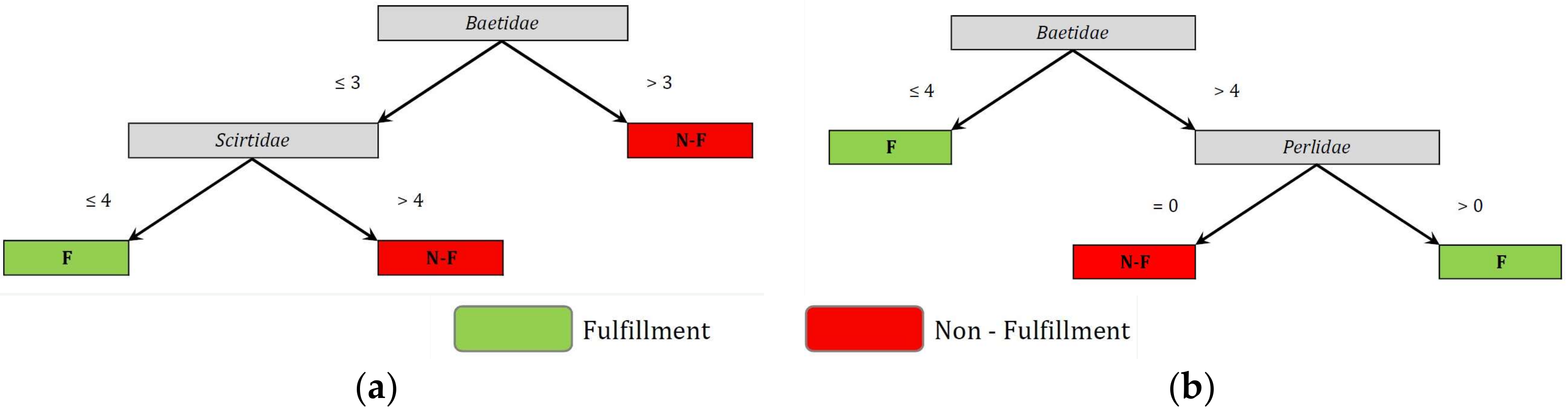
(a) Recreational Fecal Coliform Regulation
Model: 1a4Models: 1a5, 1a6, 1a7
Baetidae <= 3: A
Baetidae > 3
| Perlidae  = 0: B
| Perlidae  > 0
| | Chironomidae <= 3: B
| | Chironomidae  > 3: A
Baetidae <= 3
| Scirtidae = 1: A
| Scirtidae > 1: B
Baetidae > 3: B
Model: 1a8Models: 1a9, 1a10, 1a11, 1a12
Baetidae <= 3
| Elminthidae <= 2: A
| Elminthidae > 2: B
Baetidae > 3: B
Baetidae <= 3
| Scirtidae <= 4: A
| Scirtidae > 4: B
Baetidae > 3: B
(b) Agriculture fecal coliform regulation
Model: 2ap3Models: 2ap4, 2ap5
Perlidae  = presence: A
Perlidae  = absence
| Baetidae = presence
| | Leptophlebiidae = presence: A
| | Leptophlebiidae = absence: B
| Baetidae = absence: A
Perlidae = presence: A
Perlidae = absence
| Baetidae = presence: B
| Baetidae = absence: A
Models: 2a1, 2a2, 2a3, 2a4, 2a5, 2a6Models: 2a7, 2a8, 2a9, 2a10, 2a11
Baetidae <= 4: A
Baetidae > 4
| Perlidae = 0: B
| Perlidae > 0: A
Perlidae = 0
| Baetidae <= 4: A
| Baetidae > 4: B
Perlidae > 0: A
A: fulfillment; B: non-fulfillment

References

  1. Gofti-Laroche, L.; Demanse, D.; Joret, J.-C.; Zmirou, D. Health risks and parasitical quality of water. J. Am. Water Works Assoc. 2003, 95, 162–172. [Google Scholar] [CrossRef]
  2. World Health Organization (WHO). Guidelines for Drinking-Water Quality; World Health Organization: Geneva, Switzerland, 2004; Volume 1. [Google Scholar]
  3. Mallin, M.A.; Johnson, V.L.; Ensign, S.H.; MacPherson, T.A. Factors contributing to hypoxia in rivers, lakes, and streams. Limnol. Oceanogr. 2006, 51, 690–701. [Google Scholar] [CrossRef]
  4. Arnone, R.D.; Walling, J.P. Waterborne pathogens in urban watersheds. J. Water Health 2007, 5, 149–162. [Google Scholar] [CrossRef] [PubMed]
  5. Oliver, B.G. Guidelines for Drining-Water Quality, Volume 1: Recommendations; Elsevier: Geneva, Switzerland, 1984; p. 130. [Google Scholar]
  6. Fewtrell, L.; Bartram, J.; Organization, W.W.H. Water Quality: Guidelines, Standards, and Health: Assessment of Risk and Risk Management for Water-Related Infectious Disease; IWA Publishing: London, UK, 2001. [Google Scholar]
  7. World Health Organization (WHO). Guidelines for Safe Recreational Water Environments: Coastal and Fresh Waters; World Health Organization: Geneva, Switzerland, 2003; Volume 1. [Google Scholar]
  8. Dominguez-Granda, L.; Lock, K.; Goethals, P.L. Using multi-target clustering trees as a tool to predict biological water quality indices based on benthic macroinvertebrates and environmental parameters in the Chaguana Watershed (Ecuador). Ecol. Inform. 2011, 6, 303–308. [Google Scholar] [CrossRef]
  9. De Pauw, N.; Gabriels, W.; Goethals, P.L. River monitoring and assessment methods based on macroinvertebrates. In Biological Monitoring of Rivers: Applications and Perspectives; John Wiley and Son, Ltd.: Chichester, UK, 2006; pp. 113–134. [Google Scholar]
  10. Gabriels, W.; Lock, K.; De Pauw, N.; Goethals, P.L. Multimetric macroinvertebrate index Flanders (MMIF) for biological assessment of rivers and lakes in Flanders (Belgium). Limnol. Ecol. Manag. Inland Waters 2010, 40, 199–207. [Google Scholar] [CrossRef]
  11. Džeroski, S.; Demšar, D.; Grbović, J. Predicting chemical parameters of river water quality from bioindicator data. Appl. Intell. 2000, 13, 7–17. [Google Scholar] [CrossRef]
  12. Griffiths, M. The European water framework directive: An approach to integrated river basin management. Eur. Water Manag. Online 2002, 5, 1–14. [Google Scholar]
  13. Junqueira, V.; Campos, S. Adaptation of the “BMWP” method for water quality evaluation to Rio das Velhas watershed (Minas Gerais, Brazil). Acta Limnol. Bras. 1998, 10, 125–135. [Google Scholar]
  14. Mustow, S. Biological monitoring of rivers in Thailand: Use and adaptation of the BMWP score. Hydrobiologia 2002, 479, 191–229. [Google Scholar] [CrossRef]
  15. Roldán Pérez, G.A. Bioindicación De La Calidad Del Agua En Colombia: Uso Del Método Bmwp/Col; Imprenta Universidad de Antioquia: Medellín, Colombia, 2003. [Google Scholar]
  16. Wilkinson, J.; Jenkins, A.; Wyer, M.; Kay, D. Modelling faecal coliform dynamics in streams and rivers. Water Res. 1995, 29, 847–855. [Google Scholar] [CrossRef]
  17. Mahloch, J.L. Comparative analysis of modeling techniques for coliform organisms in streams. Appl. Microbiol. 1974, 27, 340–345. [Google Scholar] [PubMed]
  18. Ansa, E.; Lubberding, H.; Ampofo, J.; Amegbe, G.; Gijzen, H. Attachment of faecal coliform and macro-invertebrate activity in the removal of faecal coliform in domestic wastewater treatment pond systems. Ecol. Eng. 2012, 42, 35–41. [Google Scholar] [CrossRef]
  19. Kay, D.; Mcdonald, A. Predicting coliform concentrations in upland impoundments: Design and calibration of a multivariate model. Appl. Environ. Microbiol. 1983, 46, 611–618. [Google Scholar] [PubMed]
  20. Hoang, T.H.; Lock, K.; Mouton, A.; Goethals, P.L. Application of classification trees and support vector machines to model the presence of macroinvertebrates in rivers in Vietnam. Ecol. Inform. 2010, 5, 140–146. [Google Scholar] [CrossRef]
  21. Ambelu, A.; Mekonen, S.; Koch, M.; Addis, T.; Boets, P.; Everaert, G.; Goethals, P. The application of predictive modelling for determining bio-environmental factors affecting the distribution of blackflies (diptera: Simuliidae) in the Gilgel Gibe Watershed in southwest Ethiopia. PLoS ONE 2014, 9, e112221. [Google Scholar] [CrossRef] [PubMed] [Green Version]
  22. Jerves-Cobo, R.; Everaert, G.; Iñiguez-Vela, X.; Córdova-Vela, G.; Díaz-Granda, C.; Cisneros, F.; Nopens, I.; Goethals, P.L. A methodology to model environmental preferences of EPT taxa in the Machangara River basin (Ecuador). Water 2017, 9, 195. [Google Scholar] [CrossRef]
  23. Holguin-Gonzalez, J.E.; Boets, P.; Alvarado, A.; Cisneros, F.; Carrasco, M.C.; Wyseure, G.; Nopens, I.; Goethals, P.L.M. Integrating hydraulic, physicochemical and ecological models to assess the effectiveness of water quality management strategies for the River Cuenca in Ecuador. Ecol. Model. 2013, 254, 1–14. [Google Scholar] [CrossRef]
  24. Acosta, R.; Hampel, H. Evaluación Del Estado Ecológico Y Biodiversidad De Macroinvertebrados Bentónicos En La Cuenca Alta Del Río Paute Y Parque Nacional El Cajas; Universidad de Cuenca: Cuenca, Ecuador, 2015; p. 83. [Google Scholar]
  25. Goethals, P.; Dedecker, A.; Gabriëls, W.; De Pauw, N. Development and application of predictive river ecosystem models based on classification trees and artificial neural networks. In Ecological Informatics; Springer: Berlin, Germany, 2006; pp. 151–167. [Google Scholar]
  26. Ambelu, A.; Lock, K.; Goethals, P. Comparison of modelling techniques to predict macroinvertebrate community composition in rivers of Ethiopia. Ecol. Inform. 2010, 5, 147–152. [Google Scholar] [CrossRef]
  27. Dakou, E.; D’Heygere, T.; Dedecker, A.P.; Goethals, P.L.M.; Lazaridou-Dimitriadou, M.; De Pauw, N. Decision tree models for prediction of macroinvertebrate taxa in the river axios (northern greece). Aquat. Ecol. 2007, 41, 399–411. [Google Scholar] [CrossRef]
  28. Goethals, P. Data Driven Development of Predictive Ecological Models for Benthic Macroinvertebrates in Rivers; Ghent University: Ghent, Belgium, 2005. [Google Scholar]
  29. Fernandez de Cordova, J.; González, H. Evoluación De La Calidad Del Agua De Los Tramos Bajos De Los Ríos De La Ciudad De Cuenca; ETAPA-EP: Cuenca, Ecuador, 2012. [Google Scholar]
  30. Instituto Nacional de Estadísticas y Censos del Ecuador (INEC). Proyección De La Población Ecuatoriana, Por Años Calendario, Según Cantones 2010–2020; Instituto Nacional de Estadísticas y Censos del Ecuador: Quito, Ecuador, 2010.
  31. PROMAS-UCuenca. Información de la Red Meteorológica e Hidrológica. Progarma para el Manejo del Agua y el Suelo; Universidad de Cuenca: Cuenca, Ecuador, 2010. [Google Scholar]
  32. Aereopuerto-Mariscal-Lamar. Información Meteorológica Aereopuerto Mariscal Lamar Cuenca; Dirección de Aviación Civil del Ecuador: Quito, Ecuador, 2012.
  33. Estrella, R.; Tobar, V. Hidrologia Y Climatologia—Formulación Del Plan De Manejo Integral De La Subcuenca Del Río Machangara; ACOTECNIC Cia. Ltda.—Consejo de Cuenca del Río Machangara: Cuenca, Ecuador, 2013. [Google Scholar]
  34. Esquivel, J.C.; Verbeiren, B.; Alvarado, A.; Feyen, J.; Cisneros, F. Preliminary statistical analysis of the water quality database of ETAPA; PROMAS—Universidad de Cuenca: Cuenca, Ecuador, 2008. [Google Scholar]
  35. Mulliss, R.; Revitt, D.M.; Shutes, R.B.E. The impacts of discharges from two combined sewer overflows on the water quality of an urban watercourse. Water Sci. Technol. 1997, 36, 195–199. [Google Scholar]
  36. Hvitved-Jacobsen, T. The impact of combined sewer overflows on the dissolved oxygen concentration of a river. Water Res. 1982, 16, 1099–1105. [Google Scholar] [CrossRef]
  37. Weyrauch, P.; Matzinger, A.; Pawlowsky-Reusing, E.; Plume, S.; von Seggern, D.; Heinzmann, B.; Schroeder, K.; Rouault, P. Contribution of combined sewer overflows to trace contaminant loads in urban streams. Water Res. 2010, 44, 4451–4462. [Google Scholar] [CrossRef] [PubMed]
  38. Passerat, J.; Ouattara, N.K.; Mouchel, J.-M.; Vincent, R.; Servais, P. Impact of an intense combined sewer overflow event on the microbiological water quality of the seine river. Water Res. 2011, 45, 893–903. [Google Scholar] [CrossRef] [PubMed]
  39. Novotny, V. Diffuse pollution from agriculture—A worldwide outlook. Water Sci. Technol. 1999, 39, 1–13. [Google Scholar]
  40. Dohner, E.; Markowitz, A.; Barbour, M.; Simpson, J.; Byrne, J.; Dates, G. Volunteer Stream Monitoring: A Methods Manual; Environmental Protection Agency: Washington, DC, USA, 1997.
  41. Armitage, P.D.; Moss, D.; Wright, J.F.; Furse, M.T. The performance of a new biological water quality score system based on macroinvertebrates over a wide range of unpolluted running-water sites. Water Res. 1983, 17, 333–347. [Google Scholar] [CrossRef]
  42. Sutherland, W.J. Ecological Census Techniques: A Handbook; Cambridge University Press: New York, NY, USA, 2006. [Google Scholar]
  43. Alba-Tercedor, J.; Pardo, I.; Prat, N.; Pujante, A. Protocolos de muestreo y análisis para invertebrados bentónicos. In Metodología Para el Establecimiento del Estado Ecológico Según la Directiva Marco del Agua; Ministerio de Medio Ambiente, Confederación Hidrográfica del Ebro: Madrid, España, 2005; pp. 131–175. (in Spanish) [Google Scholar]
  44. Roldán Pérez, G.A. Guía Para El Estudio De Los Macroinvertebrados Acuáticos Del Departamento De Antioquia; Fondo para la Protección del Medio Ambiente “José Celestino Mutis”: Bogotá, Colombia, 1988.
  45. Álvarez, L.F. Metodología Para La Utilización De Los Macroinvertebrados Acuáticos Como Indicadores De La Calidad Del Agua; Instituto de Investigación de Recursos Biológicos Alexander von Humboldt: Bogotá, Colombia, 2005. [Google Scholar]
  46. Encalada, A.C.; Sant, M.R.; Prat i Fornells, N.; Quito, U.S.F.d.; Barcelona, U.d.; Desarrollo, A.E.d.C.I.p.e.; Agua, F.p.l.P.d. Protocolo Simplificado Y Guía De Evaluación De La Calidad Ecológica De Ríos Andinos (Cera-S): text 2. Làmines; Proyecto FUCARA: Quito, Ecuador, 2011. [Google Scholar]
  47. Zúñiga, M.d.C.; Cardona, W.; Cantera, J.; Carvajal, Y.; Castro, L. Bioindicadores de calidad de agua y caudal ambiental. In Caudal Ambiental: Conceptos, Experiencias y Desafíos; Universidad del Valle: Cali, Colombia, 2009; Volume 1, pp. 303–310. [Google Scholar]
  48. MAE-Ecuador. Tulas—Texto Unificado de Legislación Secundaria; Ministerio-del-Ambiente, Ed.; EDICION ESPECIAL No. 270 ed.; Acuerdo Ministerial No. 028; Registro Oficial: Quito, Ecuador, 2015.
  49. Sánchez, L.; Sánchez, A.; Galvis, G.; Latorre, J. Filtración en Múltiples Etapas; IRC International Water and Sanitation Centre: Delft, The Netherlands, 2007; Volume 15. [Google Scholar]
  50. Quinlan, J.R. Induction of decision trees. Mach. Learn. 1986, 1, 81–106. [Google Scholar] [CrossRef]
  51. Quinlan, J.R. Generating production rules from decision trees. In Proceedings of the 10th International Joint Conference on Artificial Intelligence, Milan, Italy, 23–29 August 1987; Morgan Kaufmann Publishers Inc.: San Francisco, CA, USA, 1987; pp. 304–307. [Google Scholar]
  52. Everaert, G.; Boets, P.; Lock, K.; Džeroski, S.; Goethals, P.L. Using classification trees to analyze the impact of exotic species on the ecological assessment of polder lakes in flanders, belgium. Ecol. Model. 2011, 222, 2202–2212. [Google Scholar] [CrossRef]
  53. Lior, R. Data Mining with Decision trees: Theory and Applications; World Scientific: Singapore, 2014; Volume 81. [Google Scholar]
  54. Forio, M.A.E.; Van Echelpoel, W.; Dominguez-Granda, L.; Mereta, S.T.; Ambelu, A.; Hoang, T.H.; Boets, P.; Goethals, P.L.M. Analysing the effects of water quality on the occurrence of freshwater macroinvertebrate taxa among tropical river basins from different continents. AI Commun. 2016, 29, 665–685. [Google Scholar] [CrossRef]
  55. Stockwell, D.R.; Peterson, A.T. Effects of sample size on accuracy of species distribution models. Ecol. Model. 2002, 148, 1–13. [Google Scholar] [CrossRef]
  56. Yu, R.; Abdel-Aty, M. Utilizing support vector machine in real-time crash risk evaluation. Accid. Anal. Prev. 2013, 51, 252–259. [Google Scholar] [CrossRef] [PubMed]
  57. Moisen, G. Classification and regression trees. In Encyclopedia of Ecology; Elsevier: Oxford, UK, 2008; pp. 582–588. [Google Scholar]
  58. Witten, I.H.; Frank, E. Data Mining: Practical Machine Learning Tools and Techniques; Morgan Kaufmann: San Francisco, CA, USA, 2005. [Google Scholar]
  59. Quinlan, J.R. C4. 5: Programs for Machine Learning; Elsevier: San Mateo, CA, USA, 2014. [Google Scholar]
  60. Goethals, P.L.; Dedecker, A.P.; Gabriels, W.; Lek, S.; De Pauw, N. Applications of artificial neural networks predicting macroinvertebrates in freshwaters. Aquat. Ecol. 2007, 41, 491–508. [Google Scholar] [CrossRef]
  61. Fielding, A.H.; Bell, J.F. A review of methods for the assessment of prediction errors in conservation presence/absence models. Environ. Conserv. 1997, 24, 38–49. [Google Scholar] [CrossRef]
  62. Ting, K.M. An instance-weighting method to induce cost-sensitive trees. IEEE Trans. Knowl. Data Eng. 2002, 14, 659–665. [Google Scholar] [CrossRef]
  63. Maimon, O.; Rokach, L. Data Mining and Knowledge Discovery Handbook; Springer: New York, NY, USA, 2005; Volume 2. [Google Scholar]
  64. Kohavi, R.; Provost, F. Glossary of terms. Mach. Learn. 1998, 30, 271–274. [Google Scholar]
  65. Fukuda, S.; De Baets, B.; Mouton, A.M.; Waegeman, W.; Nakajima, J.; Mukai, T.; Hiramatsu, K.; Onikura, N. Effect of model formulation on the optimization of a genetic takagi–sugeno fuzzy system for fish habitat suitability evaluation. Ecol. Model. 2011, 222, 1401–1413. [Google Scholar] [CrossRef]
  66. Cohen, J. A coefficient of agreement for nominal scales. Educ. Psychol. Meas. 1960, 20, 37–46. [Google Scholar] [CrossRef]
  67. Landis, J.R.; Koch, G.G. The measurement of observer agreement for categorical data. Biometrics 1977, 33, 159–174. [Google Scholar] [CrossRef] [PubMed]
  68. Wei, J.-M.; Yuan, X.-J.; Hu, Q.-H.; Wang, S.-Q. A novel measure for evaluating classifiers. Expert Syst. Appl. 2010, 37, 3799–3809. [Google Scholar] [CrossRef]
  69. Everaert, G.; Pauwels, I.S.; Boets, P.; Verduin, E.; de la Haye, M.A.A.; Blom, C.; Goethals, P.L.M. Model-based evaluation of ecological bank design and management in the scope of the european water framework directive. Ecol. Eng. 2013, 53, 144–152. [Google Scholar] [CrossRef]
  70. Everaert, G.; Pauwels, I.S.; Boets, P.; Buysschaert, F.; Goethals, P.L. Development and assessment of ecological models in the context of the european water framework directive: Key issues for trainers in data-driven modeling approaches. Ecol. Inform. 2013, 17, 111–116. [Google Scholar] [CrossRef]
  71. Džeroski, S.; Grbović, J.; Walley, W.J.; Kompare, B. Using machine learning techniques in the construction of models. Ii. Data analysis with rule induction. Ecol. Model. 1997, 95, 95–111. [Google Scholar] [CrossRef]
  72. Roldán Pérez, G. Los macroinvertebrados y su valor como indicadores de la calidad del agua. Acad. Colomb. Cienc. 1999, 23, 375–387. [Google Scholar]
  73. Jacobsen, D. The effect of organic pollution on the macroinvertebrate fauna of ecuadorian highland streams. Archiv für Hydrobiol. 1998, 143, 179–195. [Google Scholar] [CrossRef]
  74. Ríos-Touma, B.; Encalada, A.C.; Prat Fornells, N. Macroinvertebrate assemblages of an andean high-altitude tropical stream: The importance of season and flow. Int. Rev. Hydrobiol. 2011, 96, 667–685. [Google Scholar] [CrossRef]
  75. Jacobsen, D. Temporally variable macroinvertebrate–stone relationships in streams. Hydrobiologia 2005, 544, 201–214. [Google Scholar] [CrossRef]
  76. Burneo, P.C.; Gunkel, G. Ecology of a high andean stream, río Itambi, Otavalo, Ecuador. Limnol. Ecol. Manag. Inland Waters 2003, 33, 29–43. [Google Scholar] [CrossRef]
  77. Dallas, H.F.; Day, J.A. Natural variation in macroinvertebrate assemblages and the development of a biological banding system for interpreting bioassessment data—A preliminary evaluation using data from upland sites in the south-western Cape, South Africa. Hydrobiologia 2007, 575, 231–244. [Google Scholar] [CrossRef]
  78. Kauffman, J.B.; Krueger, W.C. Livestock impacts on riparian ecosystems and streamside management implications… A review. J. Range Manag. 1984, 37, 430–438. [Google Scholar] [CrossRef]
  79. Seyfried, P.; Harris, E. Bacteriological Characterization of Feces and Source Differentiation; Water Resources Branch, Ontario Ministry of the Environment: Toronto, ON, Canada, 1990.
  80. Leclerc, H.; Mossel, D.; Edberg, S.; Struijk, C. Advances in the bacteriology of the coliform group: Their suitability as markers of microbial water safety. Ann. Rev. Microbiol. 2001, 55, 201–234. [Google Scholar] [CrossRef] [PubMed]
  81. Tallon, P.; Magajna, B.; Lofranco, C.; Leung, K.T. Microbial indicators of faecal contamination in water: A current perspective. Water Air Soil Pollut. 2005, 166, 139–166. [Google Scholar] [CrossRef]
  82. Wade, T.J.; Calderon, R.L.; Sams, E.; Beach, M.; Brenner, K.P.; Williams, A.H.; Dufour, A.P. Rapidly measured indicators of recreational water quality are predictive of swimming-associated gastrointestinal illness. Environ. Health Perspect. 2006, 114, 24–28. [Google Scholar] [CrossRef] [PubMed]
  83. Forio, M.A.E.; Landuyt, D.; Bennetsen, E.; Lock, K.; Nguyen, T.H.T.; Ambarita, M.N.D.; Musonge, P.L.S.; Boets, P.; Everaert, G.; Dominguez-Granda, L.; et al. Bayesian belief network models to analyse and predict ecological water quality in rivers. Ecol. Model. 2015, 312, 222–238. [Google Scholar] [CrossRef]
Figure 1. Location of the Machangara basin in Ecuador.
Water 10 00375 g001
Figure 2. Sampled sites location with (a) land use; (b) Biological Monitoring Working Party score adapted to Colombia (BMWP-Col) qualification.
Water 10 00375 g002
Figure 3. Boxplots of the fecal coliforms variation according to land use.
Water 10 00375 g003
Figure 4. Fulfillment of fecal coliforms limits in relation to water use. (a) Recreational with primary contact; (b) Agricultural and livestock use; (c) For raw water use previous to non-conventional treatment required.
Water 10 00375 g004
Figure 5. Macroinvertebrates abundance decision tree models (DTMs) in relation to fecal coliforms water use standard. Fulfillment of: (a) primary contact and (b) agriculture and livestock irrigation.
Water 10 00375 g005
Table 1. Ecuadorian Water Quality Regulation for fecal coliforms [48].
RegulationsWater Used forFecal Coliforms Limited Value MPN.100 mL−1
RecreationalRecreational with primary contact≤200
AgricultureAgriculture and livestock≤1000
Raw waterRaw water previous to non-conventional treatment a≤2000
a Conventional treatment refers to chemical addition, rapid mixing, flocculation and sedimentation; MPN = Most probable number.
Table 2. Abundance of the taxa present in sampling sites in the Machangara River during February and March of 2012.
Sampled Points in the Machangara RiverPoints with the Same Taxa
SiteSensitivity Score ↓3413151920242526272829303132333435363738394041424344454647495051
Taxa
Biological Water Quality BMWP-Col →69577159354858825574634640291964553949335938341186737578256932911
Land use category → 555354356366363622222111155536535
Tubificidae13811 111111 1 111 11111111111111128
Chironomidae238415694 6 244 2 11524026 94315823223104 27
Dytiscidae3 1 1
Physidae3 14 1 13
Glossiphoniidae3 1 1 11 3 1 6
Empididae4 1 1
Psychodidae4 1 1
Hydrophilidae4 1 1
Planorbidae4 1 2 2
Dixidae4 1 1 2
Limoniidae4 3 5 3 3
Tabanidae4 1 1 1 3
Limnaeidae4 1 1 2 2 4
Ceratopogonidae41 11 2 1 1 6
Planariidae4 6 1 14 2 1611 8
Staphylinidae5 2 1
Hydropsychidae51 1 1 3
Muscidae5 1 2155 2 32 3 1 10
Tipulidae5 1645 21 3 11 1 3 1 1 1 14
Baetidae531337 243162383211 35371894510815131171913430 140 27
Scirtidae6 13211 231 1 1144 2 12
Elminthidae622 3 162 31151 24 1 1 411 17
Simuliidae61833131212312619458 1851451221011421 1815315 27
Aeshnidae7 1 1 2
Tricorythidae7257 62328 1 114 9 12 13
Hyalellidae7884 6307 101163 2 3 21 1 62221166138522
Leptoceridae8 1 1 1 1 1 2 6
Leptophlebiidae810 4 1265 1 2 56 9
Hydrobiosidae82364 21 91 1 1422 11116 17
Helicopsychidae9 1 1
Ptilodactylidae9 1 1 2
Odontoceridae9 1 1 2
Hydracarina10 1 1 2
Blepharoceridae10 1 1 2
Gripopterygidae10 1 1 2
Calamoceratidae102 1 1 1 4
Perlidae10 17 61 4111 1 1 1 9 12
Taxa richness →121011108109141013108764121271181177431271114111473
Land use category → 1Urban area2Suburban area, pastures and crops3Pastures4Bare soil5Native vegetation6Forest vegetation
Biological water quality classification → Very good Good Moderate Deficient Bad
Taxa analyzed to construct the models → Included Not included p = Taxa present
Table 3. Predictive results from models developed during the models development phase that were based on the J4.8 algorithm pruned tree (before optimization): correctly classified instances (CCI), Kappa statistics and overall confusion entropy of a confusion matrix (CEN).
Model No.FCR aModel SettingsModel Outcomes
CCI c (%)Kappa StatisticsNumber of LeavesCEN d
J4.8PCF bMean ± sdMean ± sdMean ± sd
1eapf1gRecreational h3, 5 and 10 fcv i0.2540.40 ± 3.50−0.21 ± 0.0961.03 ± 0.01
1ap2Recreational3, 5 and 10 fcv0.1048.48 ± 3.03−0.09 ± 0.0721.01 ± 0.02
1a1Recreational3, 5, 10 fcv and 66%tr0.2570.45 ± 1.500.39 ± 0.0550.81 ± 0.03
1a2Recreational3, 5, 10 fcv and 66%tr0.1070.45 ± 1.500.39 ± 0.0540.81 ± 0.03
2ap1Agriculture3, 5 and 10 fcv0.2566.67 ± 0.000.17 ± 0.0340.88 ± 0.01
2ap2Agriculture j3, 5 and 10 fcv0.1069.70 ± 3.030.24 ± 0.0030.84 ± 0.01
2a1Agriculture3, 5, 10 fcv and 66%tr0.2586.35 ± 7.990.68 ± 0.1930.52 ± 0.20
2a2Agriculture3, 5, 10 fcv and 66%tr0.1077.25 ± 16.870.43 ± 0.4430.67 ± 0.26
Mean and standard deviations of CCI, Kappa statistics and CEN were derived from k-fold cross validation. In the case of two or more models that had the same DTM, these parameters were obtained from a k-fold cross validation of all related models. a FCR = Fecal coliform regulation; b PCF = Pruning confidence factor; c CCI= Correctly classified instances; d CEN = Overall confusion entropy of a confusion matrix; e fecal coliform regulation: 1 for recreational and 2 for agriculture; f The kind of database: ap = absence/presence, a = abundance; g The number of model with different value of PCF; h The short name of FCR; i fcv = folds cross validation; j Models obtained from agriculture regulation could be applied to check the raw water fecal regulation.
Table 4. Summary of the predictive result of the models with the best accuracy after optimization, in which the cost matrix weights was used: correctly classified instances (CCI), Kappa statistics and overall confusion entropy of a confusion matrix (CEN).
Model No.Model SettingsModel Outcomes
J4.8PCF aCMW bCCI g (%)Kappa StatisticsCEN h
TP cFN dFP eTN fMean ± sdMean ± sdMean ± sd
1iaj-4k3, 5 and 10 fcv l0.25012072.73 ± 6.050.44 ± 0.130.78 ± 0.09
1a5 to 1a73, 5 and 10 fcv0.25013 to 5077.43 ± 8.030.56 ± 0.150.64 ± 0.11
1a83, 5 and 10 fcv0.25017078.77 ± 8.000.58 ± 0.150.61 ± 0.11
1a9 to 1a123, 5 and 10 fcv0.1 and 0.25018 and 9074.93 ± 6.930.51 ± 0.130.67 ± 0.07
2ap33, 5 and 10 fcv0.25012075.76 ± 5.250.47 ± 0.130.67 ± 0.15
2ap4 and 2ap53, 5 and 10 fcv0.25013 and 5072.73 ± 7.170.43 ± 0.130.68 ± 0.10
2a3 to 2a63, 5 and 10 fcv0.25011 to 4087.12 ± 6.590.69 ± 0.160.53 ± 0.16
2a7 to 2a113, 5 and 10 fcv0.25015 to 15080.21 ± 9.440.56 ± 0.190.63 ± 0.13
Mean and standard deviations of CCI, Kappa statistics and CEN were derived from k-fold cross validation. a PCF = Pruning confidence factor; b CMW = Cost Matrix Weights; c TP = True positives; d FN = False negative; e FP = False positive; f TN = True negative; g CCI = Correctly classified instances; h CEN = Overall confusion entropy of a confusion matrix; i Fecal coliform regulation: 1 for recreational and 2 for agriculture; j Kind of database: ap = absence/presence, a = abundance; k Number of model with different value of PCF; l fcv = folds cross validation.

