Comprehensive Forecast of Urban Water-Energy Demand Based on a Neural Network Model


1
State Key Laboratory of Hydrology-Water Resources and Hydraulic Engineering, Nanjing Hydraulic Research Institute, Nanjing 210029, China
2
The College of Water Conservancy and Hydropower Engineering, Hohai University, Nanjing 210098, China
*
Author to whom correspondence should be addressed.
Water 2018, 10(4), 385; https://doi.org/10.3390/w10040385
Submission received: 25 January 2018
/
Revised: 18 March 2018
/
Accepted: 21 March 2018
/
Published: 26 March 2018
(This article belongs to the Special Issue Water Quality: A Component of the Water-Energy-Food Nexus)
Abstract
:Water-energy nexus has been a popular topic of rese arch in recent years. The relationships between the demand for water resources and energy are intense and closely connected in urban areas. The primary, secondary, and tertiary industry gross domestic product (GDP), the total population, the urban population, annual precipitation, agricultural and industrial water consumption, tap water supply, the total discharge of industrial wastewater, the daily sewage treatment capacity, total and domestic electricity consumption, and the consumption of coal in industrial enterprises above the designed size were chosen as input indicators. A feedforward artificial neural network model (ANN) based on a back-propagation algorithm with two hidden layers was constructed to combine urban water resources with energy demand. This model used historical data from 1991 to 2016 from Wuxi City, eastern China. Furthermore, a multiple linear regression model (MLR) was introduced for comparison with the ANN. The results show the following: (a) The mean relative error values of the forecast and historical urban water-energy demands are 1.58 % and 2.71%, respectively; (b) The predicted water-energy demand value for 2020 is 4.843 billion cubic meters and 47.561 million tons of standard coal equivalent; (c) The predicted water-energy demand value in the year 2030 is 5.887 billion cubic meters and 60.355 million tons of standard coal equivalent; (d) Compared with the MLR, the ANN performed better in fitting training data, which achieved a more satisfactory accuracy and may provide a reference for urban water-energy supply planning decisions.
1. Introduction
Water and energy are basic natural and strategic resources, and they form the material basis for the survival of human society and provide an important guarantee for the sustainable development of the national economy. At present, the water-energy nexus is the focus of research by domestic and foreign scholars [1,2,3,4,5,6]. With intensified global climate change, population growth, and rapid economic and social development, the comprehensive forecast of water and energy demand in urban areas is of great significance for policy planning. In the study of water demand forecasting, Cengiz Koç forecasted the water demand of the Bodrum Peninsula for the next 3 to 40 years of the tourism season based on the local population statistics [7]. The study only analyzed the impacts of population size and structure of water demand, and it did not take into account the constraints of other economic factors on water use. Rathnayaka established Australian urban households as water terminals, divided residential end-use water into different types, established the urban residential end-use water demand model, and verified it on a time scale by the quarter and year [8]. The model only predicted the urban domestic water use without considering industrial, agricultural, and other departments of the water forecast.
In the energy demand forecast study, two fundamental approaches called the top-down and the bottom-up approach have been identified to model the residential sector’s energy consumption [9]. Ghiassi studied the bottom-up approach for urban energy computing supported by multivariate cluster analysis and introduced a two-step approach involving a reductive phase and a re-diversification process [10]. These methods were applied to forecast the energy demand without studying the relationship between water and energy instead of taking the relevant constraints of water resources into account.
Over the last decade, artificial intelligence (AI) techniques have been increasingly used in different fields for fitting and forecasting. In many quantitative structure-property studies, the multiple linear regression (MLR) method is commonly used; however, this method also presents certain limitations when working with a complex system. The flexibility of an artificial neural network (ANN) model can be used to resolve relatively complex non-linear issues. Tiantian Yang et al. used Random Forest, ANN, and Support Vector Regression methods to predict one-month-ahead reservoir inflows for two headwater reservoirs in the United States of America (USA) and China, respectively [11]. Yusuf Kurtgoz et al. estimated the thermal efficiency, brake specific fuel consumption, and volumetric efficiency values of a biogas engine operated via spark ignition at different methane ratios and engine load values with the help of the ANN model, and their study showed that ANN models generate good results for spark ignition biogas engines that present strong correlations and low error rates [12]. An improved solar forecasting algorithm based on the ANN model with fuzzy logic pre-processing was proposed, and more accurate solar irradiance forecasting results were found for Singapore [13].
Based on the nexus between water and energy, this paper overcomes the limitations of the traditional forecasting methods and improves the feedforward ANN to establish a novel model for the comprehensive forecast of urban water resources and energy demand. Also, MLR is used as a basic regression method to draw comparisons. Taking Wuxi City as an example, this paper validates the accuracy and effectiveness of the model’s prediction, reveals the quantitative connection between the two objects, and provides more intuitive and scientific data support for the nexus between water and energy.
2. Data
A water resources and energy demand integrated forecasting system is a non-linear complex system. Various factors affect the water and energy demands in urban areas and can be divided into socio-economic and natural factors [14]. Selecting the comprehensive evaluation indicators of urban water resources and energy demand should follow the principle of testability, reliability, and adequacy [15]. According to the above principles, the study uses sequential statistics from 1991 to 2016 as the basic data to access the water and energy supply and demand for Wuxi City, and the following 14 indicators based on different aspects have been selected from the Wuxi Statistical Yearbook (1991–2016) and the Water Resources Bulletin.
- (1)
- Economic and social development factors
Economic output is a major factor that affects the demand for water and energy. With continued urbanization and the implementation of the universal two-child policy, China’s urban population has grown rapidly, which has led to a corresponding increase in the demand for water and energy. This paper chose the total population (X1), urban population (X2), and the primary, secondary, and tertiary industry gross domestic product (GDP) (X3) (X4) (X5) as factors to measure the economic development.
- (2)
- Natural factors
According to water resources assessment requirements, research on the inter-annual variation of regional precipitation can provide the evidence for water resources supply and demand. In this paper, annual precipitation (X6) was used as the natural factor that influences the water demand in urban areas.
- (3)
- Use and treatment of urban water resources
Urban residents’ activities can consume and pollute many water resources. It is related to the reuse of water resources via the sewage treatment and recycling. Water consumption is usually classified into production, living, and ecological water. Given that the latter takes up quite a small proportion of water, its consumption can be disregarded. Here, agricultural (X7) and industrial water consumption (X8) are selected as water for production, while tap water supply (X9) proxied for living water consumption. Additionally, the total discharge of industrial wastewater (X10) and the daily sewage treatment capacity (X11) were used.
- (4)
- Use of major energy sources
In China, the whole of society’s energy consumption mainly relies on coal, oil, and other primary energy, which results in low efficiency and utilization and high energy consumption. Meanwhile, the total electricity consumption accounts for most of the energy consumption. The research selected total and domestic electricity consumption (X12) (X13), respectively, and the consumption of coal in industrial enterprises above a designed size (X14).
The above fourteen indices based on different aspects that influence water and energy demand were used as the indices to establish the network input.
3. Methodology
3.1. Artificial Neural Network Model
The Artificial Neural Network (ANN) is a robust, non-linear regression approach that has been extensively applied for many classification and regression problems in various fields. The learning process of the feedforward ANN with the back propagation (BP) algorithm is divided into two stages. The first stage inputs the known learning samples and calculates the output of the neurons from the first layer of the network to the following layers using the network structure and the previous iteration of the weight and threshold. The second stage modifies the weights and thresholds by calculating the effect of each weight and threshold on the total error from the last layer to the previous layers. The two processes are repeated alternately until the convergence is achieved.
The back propagation neural network algorithm with double-hidden layers (shown in Figure 1) is employed as follows:
- Step 1: Network initialization. Confirm the number of network input layer nodes n, the number of nodes in the first hidden layer l, the number of nodes in the second hidden layer p, and the number of nodes in the output layer m according to the input and output sequence (X, Y) of the system. Initialize the connection weights between the input layer, the hidden layer, and the output layer which are marked as , , and , respectively. Initialize the thresholds of the hidden layers , , the threshold of the output layer , and preset the learning rate and the neuron excitation function.
- Step 2: Calculate the hidden layer’s output. The signal that the first hidden layer transmits to the second hidden layer is as follows:The signal that the second hidden layer transmits to the output layer is as follows:The selection functions of and are written as follows:
- Step 3: Calculate the output layer’s output. The output of the BP Neural Network with double hidden layers is written as follows:
- Step 4: Calculate the errors. The network prediction error is calculated based on the network predicted output Y and the expected output T. The nodal error of the output layer is:where n is the number of output layer nodes and m is the number of input layer nodes.
- Step 5: Update the weights. The connection weights , , and are updated based on the network prediction error . The correction of the weights is conducted along the opposite direction of the gradient of the error performance function [16].
- Step 6: Update the thresholds. Update thresholds of the network node , and according to the network prediction error .
- Step 7: Determine whether the algorithm iteration ends until the global errormeets the conditions in which and , where is the preset error accuracy, n is the number of input nodes, and m is the number of output nodes, or reaches the maximum number of learning times. Then, the iteration ends. Otherwise, return to Step 2.
3.2. Model Establishment and Implementation
In this paper, the BP network functions of the MATLAB R2014b Software [17] are used to realize the establishment of the network model with double hidden layers. The BP network functions are newff (), train (), and sim (). newff () is used to design a BP network, train () is applied to train a feedforward ANN, and sim () is used to predict the functional output of a trained network. The network design is written as follows:
where P and T are the input and output matrices of the training set, respectively. S1 and S2 are the number of the first and second hidden layer nodes, respectively. TF1 and TF2 are the transfer functions of the two layers’ nodes, BTF is the training function of the network, BLF represents the learning function, and PF represents the performance analysis function. net is the value returned back to the completed BP network model. train () is used to train the network model, such as the following
net = newff (P, T, [S1, S2], {TF1, TF2}, BTF, BLF, PF)
When the network model training is complete, use the function sim () for data simulation, such as the following
where X0 is the input matrix of the test set and Y is the simulation result of the neural network. Select the mean square error of the network predicted and the expected value as a measure
where m is the number of output layer nodes; n is the number of input layer nodes. is the actual output value of the j-th output of the i-th input sample; and is the expected output value of the j-th output of the i-th input sample.
Furthermore, the multiple linear regression model (MLR) is used as a basic method to draw comparisons to the proposed ANN. We set the fourteen indices as the independent variables while the water resources demand and energy demand were defined as the dependent variables Y1 and Y2, respectively.
3.3. Multiple Linear Regression Model
Most statistical calculations are performed using linear regression models, which have been frequently applied in different fields [18,19,20]. Almost every discipline utilizes regression analyses as a basis for comparing improved models [21,22,23].
Usually, the expression formula of MLR is set as
where Y and X denote the dependent and independent variables with the number p, stands for the regression coefficient, and is the random error.
The bias measure of the MLR is the correlation coefficient (R2) for a calibration set with n samples, which is calculated as follows:
where and denote the reference and mean value for the i-th sample, respectively, and denotes the corresponding estimated value derived from the MLR model [24]. The R2 value represents the contribution of the explanatory variable to a change in the predictor variable ranging from 0 to 1. When the value closes to 1, it means the corresponding MLR model has achieved a high level of reliability [25].
4. Study Area and Experiment Design
4.1. Overview of Wuxi City, China
Wuxi is located in the south of Jiangsu Province, in the center of China’s economically developed Yangtze River Delta, and it is south of China’s third largest freshwater body, Taihu Lake. It is an important economic center, city and regional transportation hub, and represents a famous tourist destination in China. The city has a total area of 4627 km2, of which the water accounts for 1290 km2, or 27.9% of the total area. With the energy resources being relatively poor, the contradiction between energy supply and demand is increasingly acute. Coal, oil, and natural gas and other forms of primary energy are mainly supplied via nonlocal transfers, while only solar energy on behalf of renewable energy has large-scale use conditions.
4.2. Urban Water-Energy Demand Training and Forecast
We chose the data of water resources and energy in Wuxi from 1991 to 2016 as samples (See Appendix A). Typically, in the feedforward ANN, the data have to be divided into 2–3 chunks, with a segment of data reserved outside of the training phase and validation phase of the model. Then, we test the performance of the trained model on the reserved dataset as an independent test set to verify the results (overfitting, accuracy, etc.).
The fourteen impact factors from Section 2 are used here as the input indices of the network. We chose their values from 1991 to 2010 and the total water and energy consumption in the corresponding years as the training sets, while we selected the same fourteen variables from 2011 to 2016 as the test sets, aiming to verify the validity of the model. The sample data were drawn from the Wuxi Statistical Yearbook.
The training sets are divided into two subsets. One is used as a training subset to fit the parameters of the network (i.e., the gradient, weights, and bias values), which accounts for 80% of the total dataset. The other subset is known as the validation subset and is used to check for network errors during training. The latter subset accounts for 20% of the total data. The errors will be reduced in the first training stage. However, as the network begins to overfit, the errors will increase and the training needs to be stopped immediately. As a result, the network structure and parameters of the network can be obtained when the minimum validation error is achieved.
The first hidden layer includes ten process neuron nodes that are used to complete the spatial weighted aggregation and excitation output of the input signal. The second hidden layer is also made up of ten process neuron nodes and aims to improve the non-linear mapping capacities of the network. The transfer functions between the former two layers are both the logarithmic S-type transfer function logsig. Furthermore, the transfer function of the output layer is the linear function purelin. Set the network training learning rate as , the momentum factor as , and the mean square error of convergence as . The number of network training iterations is set to 10,000 times, while the interval numbers of steps of the training results is set to 200 times. The utilized network training algorithm is the Levenberg–Marquardt algorithm [26], which is the fastest algorithm to train the BP neural network and allows it overcome the shortcomings of the neural network (slow convergence speed and easiness to fall into the local minima value). After several training sessions, the network has met network error requirements to achieve convergence.
5. Results and Discussion
5.1. Results of ANN
After forming the neural network, the former 20 groups of data from the years 1991 to 2010 were set as the training set, while the rest of the data from the years 2011 to 2016 were used as the testing set. Furthermore, we used the Rolling Forecast method [27], which incorporates the previous 20 sets of data into the network, predicts the 21st group of data, and calculates the relative error. When the error meets the accuracy requirement, the results will continue to be input in the network. Then, the 22nd group will be forecasted, and the process will continuously repeat.
- (1)
- Results for the training and testing periods
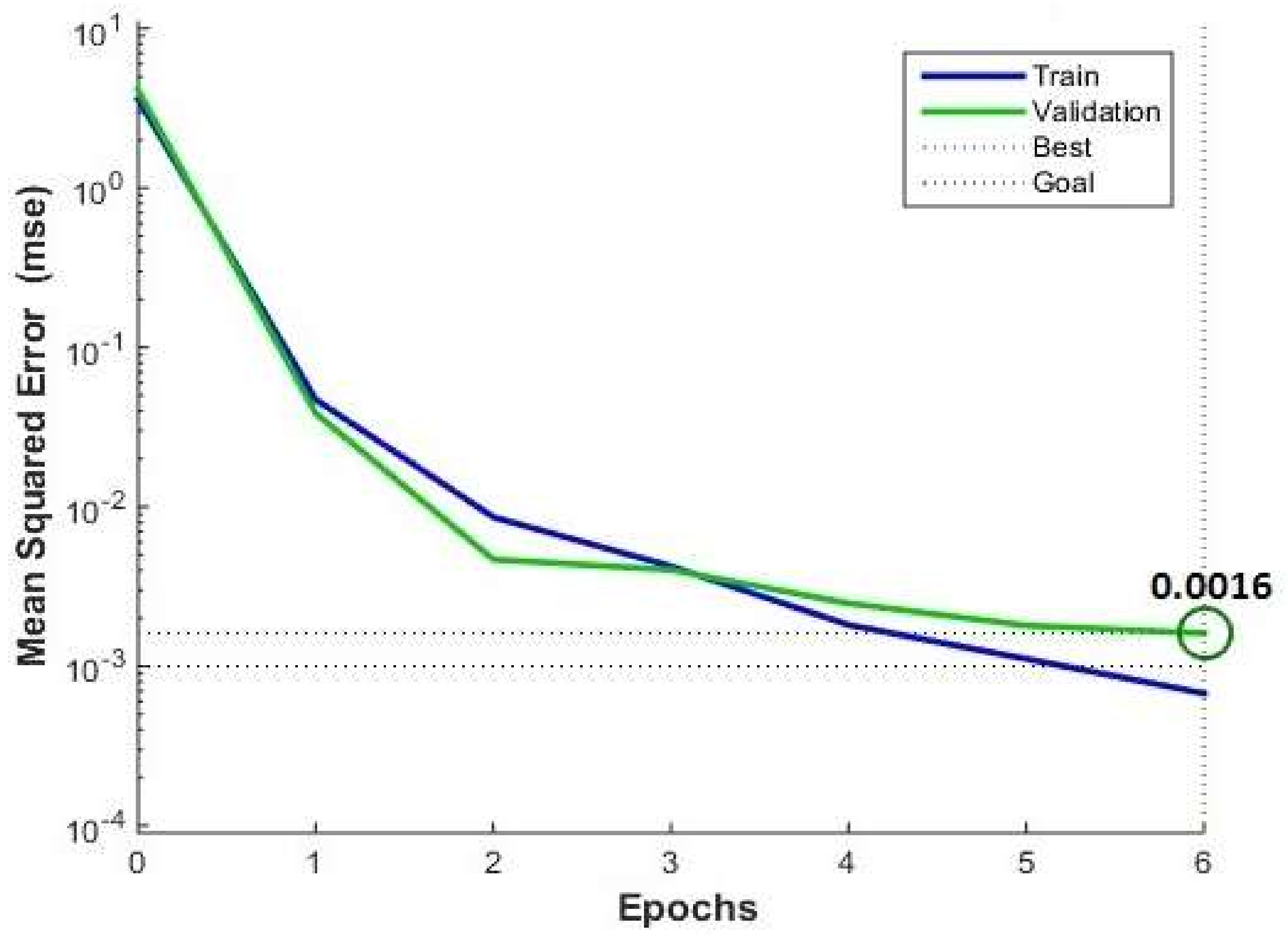
The mean relative errors (MRE) of the water and energy demand forecast from 1991 to 2016 are 1.58% and 2.71%, respectively. The neural network training performance can be seen in Figure 2. In the BP algorithm, an epoch of the net training means the finish of two stages, the forward propagation of signals, and the back propagation of errors, with the weight and threshold modified. From Figure 2, the validation shows the best performance in the 6th epoch and shows that the mean square error has reached the accuracy requirements (mse = 0.001). This finding indicates that the network training speed is quickly trained by the Levenberg–Marquardt algorithm. Additionally, the training and validation line fits well, which means that the model offers strong generalization capacities and can be applied to forecast new data.
- (2)
- Rolling forecast results
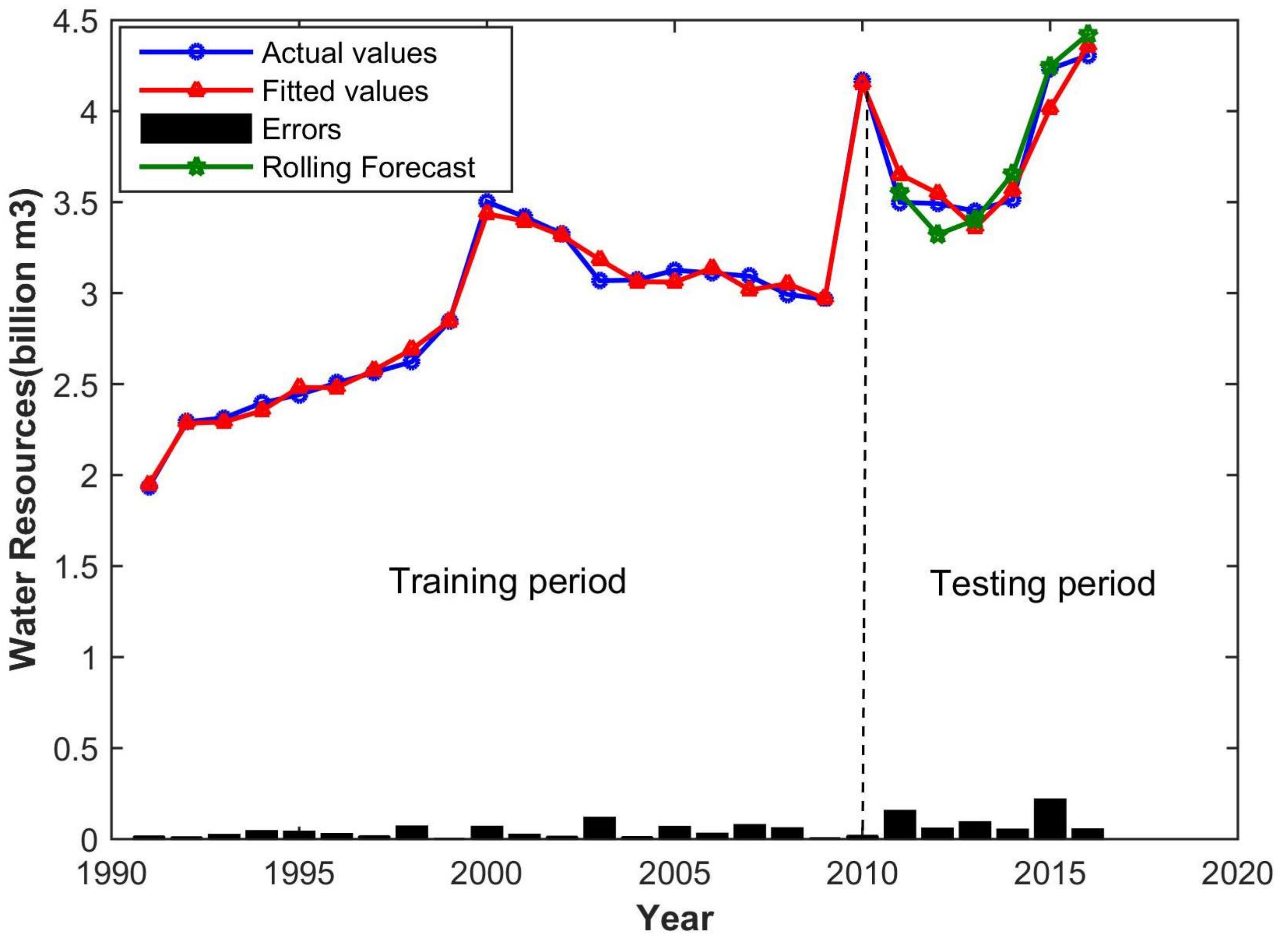
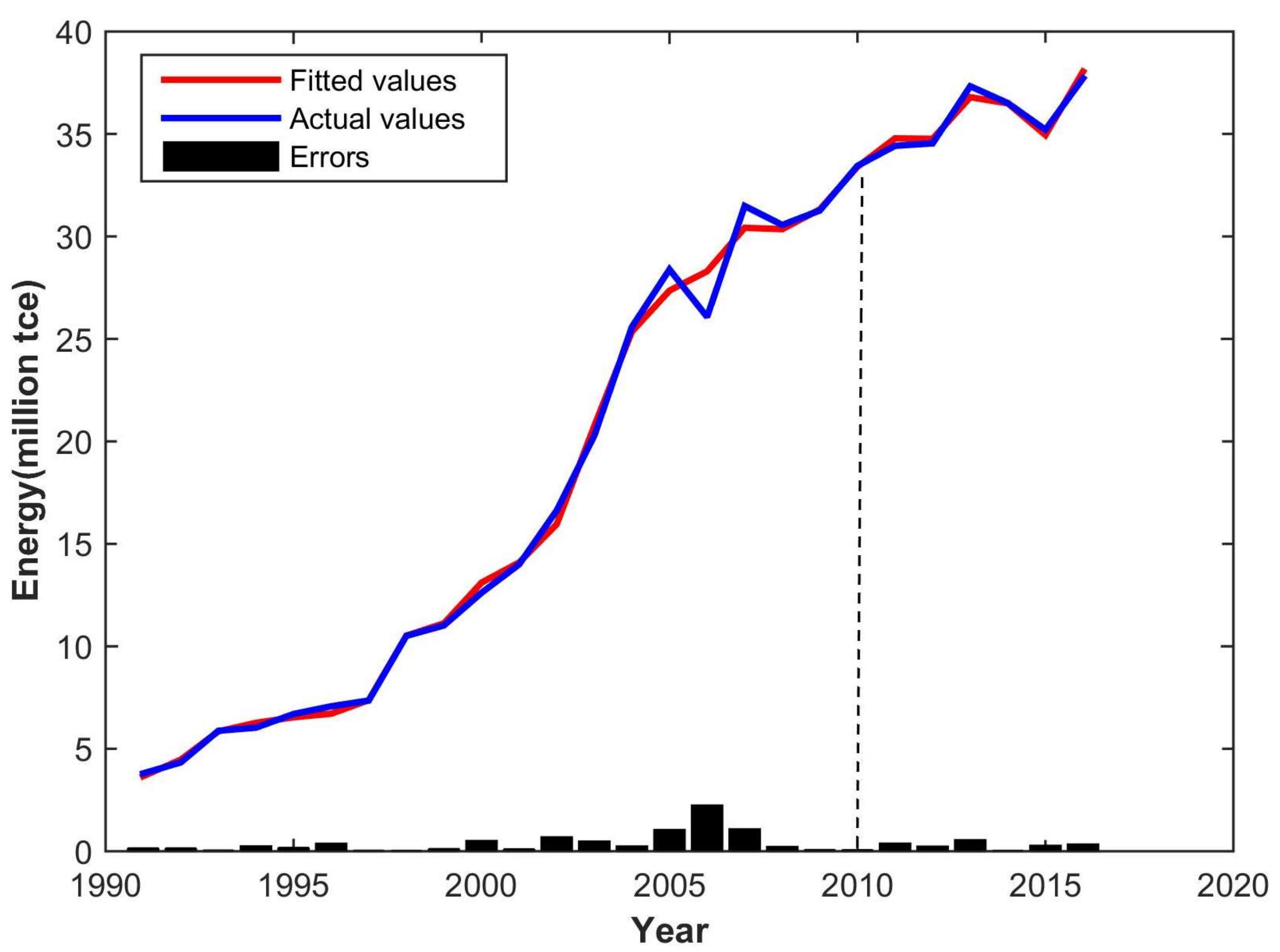
The MRE of water demand and energy demand are 2.49% and 3.95%, respectively, which indicates that the network is highly stable and adaptable and can be used to predict future demand trends.
Graphs of the actual value and forecast result of water and energy demand for Wuxi are shown in Figure 3 and Figure 4.
- (3)
- Planning level year forecast
Most of the input data for 2020 and 2030 were collected from the Wuxi’s statistical department. The primary, secondary, and tertiary industry GDP were forecast according to the average annual growth rate for the past five years.
According to a plan to further develop the Yangtze River Delta’s urban agglomerations [28], we obtained the total population index. The urban population was calculated with the urbanization rate up to 77% and 78% in year 2020 and 2030. We chose the average annual precipitation as the value in 2030 and the average for the last five years for 2020.
Tap water supply index was achieved by using the water quota of residents in the south of Jiangsu [29]. According to the plan for the construction of sewage treatment plants in Wuxi, the daily sewage treatment capacity was forecasted.
Based on the National Strategic Action Plan for Energy Development (2014–2020 Years), consumption of coal in industrial enterprises above designed size was predicted.
Other indices were forecast using the basic time series method which can be stimulated by Oracle Crystal Ball Software [30]. Due to the persistent effort in saving water in the past five years, the water consumption per ten thousand yuan for primary industry and secondary industry are both decreasing slowly, information about which can be obtained from Water Resources Bulletin of Wuxi. We forecasted the two indices with their average annual rate of decline (from 2011 to 2016) and then calculated the agricultural and industrial water consumption in 2020 and 2030.
Total discharging of industrial wastewater was done using the second exponential smoothing method [31]. An Autoregressive Integrated Moving Average Model [32] was used to derive total and domestic electricity consumption for the whole of society. We used the model to forecast the water and energy demand for 2020 and 2030 based on the data shown in Table 1 as input values. The corresponding results are shown in Table 2.
According to the 13th Five-Year Plan for Water Resources Development in Jiangsu Province [33], the province’s total water use is controlled at 52.4 billion m3 for 2020. The water demand forecast in Wuxi is forecasted to reach 4.843 billion m3 in 2020 according to the Plan for Water Resources Management in Wuxi under the Three Red Lines [34]. Compared with the planning objectives, the forecasted data calculated by the neural network model is reasonable. However, according to the 13th Five-Year Plan for Energy Development of Wuxi [35], the city has focused strictly on controlling the energy consumption intensity and the total consumption of coal. It has been vigorously applying new energy to promote a clean energy structure. As a result, the total energy demand in the future increases slowly, and even has the possibility of negative growth. Therefore, the comprehensive forecast for the network model is relatively accurate and worthy of reference.
5.2. Results of MLR
The MREs of the water and energy demand fittings are 3.88% and 2.04%, respectively.
The regression coefficients of the MLR models used to fit water resources and energy demand are shown in Table 3.
Figure 5 shows that the fitting of water resources is quite accurate on the whole, while energy fitting turns out better without considering the small errors of the middle section (Figure 6).
According to MATLAB R2014b software results, the R2 values of the water and energy demand model are 0.9279 and 0.9976, respectively, indicating that both present strong fitness.
We used the model to forecast the water and energy demand for 2020 and 2030 using the data shown in Table 1 as input values. The corresponding results are shown in Table 4. A comparison of the ANN and MLR model is shown in Table 5.
The MLR model appears to generate higher values of water and energy demand for the planning level year than that of the planning data written in documents. Overall, these results may serve as a point of comparison and offer support for the proposed ANN model.
From Table 5, we can see that the ANN model shows a better performance in fitting data of both water and energy, with a lower average MRE of 2.14% while that of MLR is 3.96%.
6. Conclusions
This paper overcomes the limitations of current traditional forecasting methods for water resources or energy demand based on the water-energy nexus via the establishment of a comprehensive forecasting model for water resources and energy demand in urban areas based on the feedforward neural network. Fourteen indices were chosen from several factors that affect the urban water and energy demand as input parameters to establish the network. The traditional BP neural network with the single hidden layer was improved by using the water resources and energy demand as the outputs. A network model with two hidden layers with local approximations and strong non-linear mapping capacities was constructed. The network can thus forecast water and energy demand.
The network model was applied to Wuxi. The average relative error values for water and energy demand forecasts were 1.58% and 2.71% for the testing period, respectively, and 2.49% and 3.95% for the rolling forecast, respectively. These results indicate that the model has strong reliability and stability.
The average MRE for water and energy demand from the ANN model was 2.14% while that of the MLR is 3.96%. Both models exhibit excellent performance. Compared with the MLR model, the proposed method indicates that the ANN can be more efficiently used to measure water and energy demand. Moreover, the results reveal the consistency and accuracy of the ANN model.
The ANN model has also been used to forecast planning years in Wuxi. The forecast results are consistent with the local planning data, which means that the model has achieved satisfactory levels of accuracy and meets the actual forecasting requirements. Thus, this model can serve as a reference of the analysis of the supply and demand balance between urban water resources and energy levels and provide a foundation for the development of water and energy planning strategies. Further studies can be conducted on the following issues:
- (a)
- The results obtained from the present study can be compared to the results obtained from different ANN training algorithms.
- (b)
- Because the ANN tends to overfit the data, other AI models such as the Support Vector Machine (SVM) and General Regression Neural Network (GRNN) can be used to draw comparisons with the ANN [36].
- (c)
- Additional data and information on the water and energy demand for Wuxi must be generated through joint efforts between government officials and researchers.
Acknowledgments
This study has been funded through the National Key R&D Program of China (Grant No. 2017YFC0404605), the International S&T Cooperation Program of China (Grant No. 2015DFA01000), and the China Postdoctoral Science Foundation Funded Project (Grant No. 2016M601847). The authors would also like to thank the editor and anonymous reviewers for their reviews and valuable comments related to this manuscript.
Author Contributions
All authors equally contributed to this paper. All authors revised and approved the final manuscript.
Conflicts of Interest
The authors declare no conflict of interest.
Nomenclature
| ANN | artificial neural network |
| MLR | multiple linear regression |
| MRE | mean relative error |
| mse | mean square error |
| RSS | residual sum of squares |
| TSS | total sum of squares |
| R2 | correlation coefficient |
| GDP | gross domestic product |
| tce | ton standard coal equivalent |
Appendix A. Training and Test Data for Water Resources and Energy of the ANN

Table A1.
Training and test data for water resources demand in Wuxi.
| Year | Water Resources Demand | |||
|---|---|---|---|---|
| Actual Value/Billion m³ | Learned Value/Billion m³ | Relative Error | ||
| Training Samples | 1991 | 1.936 | 1.950 | 0.7051 |
| 1992 | 2.293 | 2.285 | 0.3654 | |
| 1993 | 2.314 | 2.292 | 0.9408 | |
| 1994 | 2.396 | 2.353 | 1.7864 | |
| 1995 | 2.442 | 2.482 | 1.6191 | |
| 1996 | 2.507 | 2.480 | 1.0621 | |
| 1997 | 2.564 | 2.578 | 0.5616 | |
| 1998 | 2.623 | 2.691 | 2.5848 | |
| 1999 | 2.845 | 2.846 | 0.0457 | |
| 2000 | 3.502 | 3.435 | 1.9008 | |
| 2001 | 3.419 | 3.396 | 0.6751 | |
| 2002 | 3.327 | 3.315 | 0.3487 | |
| 2003 | 3.068 | 3.184 | 3.7878 | |
| 2004 | 3.072 | 3.063 | 0.3071 | |
| 2005 | 3.126 | 3.060 | 2.1009 | |
| 2006 | 3.110 | 3.138 | 0.9142 | |
| 2007 | 3.093 | 3.017 | 2.4486 | |
| 2008 | 2.993 | 3.052 | 1.9567 | |
| 2009 | 2.966 | 2.970 | 0.1287 | |
| 2010 | 4.170 | 4.153 | 0.4102 | |
| Test Samples | 2011 | 3.499 | 3.653 | 4.3990 |
| 2012 | 3.492 | 3.549 | 1.6293 | |
| 2013 | 3.451 | 3.359 | 2.6519 | |
| 2014 | 3.513 | 3.564 | 1.4428 | |
| 2015 | 4.231 | 4.014 | 5.1200 | |
| 2016 | 4.306 | 4.359 | 1.2206 | |
Table A2.
Training and test data for energy demand in Wuxi.
| Year | Energy Demand | |||
|---|---|---|---|---|
| Actual Value/Million tce | Learned Value/Million tce | Relative Error | ||
| Training Samples | 1991 | 3.800 | 3.898 | 2.5778 |
| 1992 | 4.336 | 4.422 | 1.9919 | |
| 1993 | 5.881 | 6.066 | 3.1597 | |
| 1994 | 6.033 | 6.197 | 2.7232 | |
| 1995 | 6.698 | 6.623 | 1.1217 | |
| 1996 | 7.074 | 7.463 | 5.5036 | |
| 1997 | 7.356 | 8.062 | 9.5946 | |
| 1998 | 10.508 | 9.853 | 6.2353 | |
| 1999 | 11.020 | 11.664 | 5.8382 | |
| 2000 | 12.613 | 12.823 | 1.6645 | |
| 2001 | 13.999 | 14.837 | 5.9904 | |
| 2002 | 16.632 | 16.448 | 1.1045 | |
| 2003 | 20.282 | 21.023 | 3.6497 | |
| 2004 | 25.585 | 25.435 | 0.5859 | |
| 2005 | 28.389 | 27.991 | 1.4026 | |
| 2006 | 26.071 | 26.313 | 0.9290 | |
| 2007 | 31.486 | 31.033 | 1.4407 | |
| 2008 | 30.559 | 30.725 | 0.5423 | |
| 2009 | 31.268 | 31.262 | 0.0194 | |
| 2010 | 33.447 | 33.364 | 0.2477 | |
| Test Samples | 2011 | 34.421 | 33.965 | 1.3249 |
| 2012 | 34.542 | 33.418 | 3.2525 | |
| 2013 | 37.327 | 36.657 | 1.7965 | |
| 2014 | 36.506 | 35.652 | 2.3397 | |
| 2015 | 35.206 | 35.806 | 1.7042 | |
| 2016 | 37.717 | 39.161 | 3.8272 | |
Notes: tce = ton standard coal equivalent.
References
- Hussey, K.; Pittock, J. The Energy–Water Nexus: Managing the Links between Energy and Water for a Sustainable Future. Ecol. Soc. 2012, 17, 31. [Google Scholar] [CrossRef]
- Duan, C.; Chen, B. Energy–water nexus of international energy trade of China. Appl. Energy 2017, 194, 725–734. [Google Scholar] [CrossRef]
- Valek, A.M.; Susnik, J.; Grafakos, S. Quantification of the urban water-energy nexus in Mexico City, Mexico, with an assessment of water-system related carbon emissions. Sci. Total Environ. 2017, 590, 258–268. [Google Scholar] [CrossRef] [PubMed]
- Urban, J.J. Emerging Scientific and Engineering Opportunities within the Water-Energy Nexus. Joule 2017, 1, 665–688. [Google Scholar] [CrossRef]
- Dai, J.; Wu, S.; Han, G.; Weinberg, J.; Xie, X.; Wu, X.; Song, X.; Jia, B.; Xue, W.; Yang, Q. Water-energy nexus: A review of methods and tools for macro-assessment. Appl. Energy 2018, 210, 393–408. [Google Scholar] [CrossRef]
- Vakilifard, N.; Anda, M.; Bahri, P.; Ho, G. The role of water-energy nexus in optimising water supply systems–Review of techniques and approaches. Renew. Sustain. Energy Rev. 2018, 82, 1424–1432. [Google Scholar] [CrossRef]
- Koç, C.; Bakış, R.; Bayazıt, Y. A study on assessing the domestic water resources, demands and its quality in holiday region of Bodrum Peninsula, Turkey. Tour. Manag. 2017, 62, 10–19. [Google Scholar] [CrossRef]
- Rathnayaka, K.; Malano, H.; Arora, M.; George, B.; Maheepala, S.; Nawarathna, B. Prediction of urban residential end-use water demands by integrating known and unknown water demand drivers at multiple scales II: Model application and validation. Resour. Conserv. Recycl. 2017, 118, 1–12. [Google Scholar] [CrossRef]
- Swan, L.G.; Ugursal, V.I. Modeling of end-use energy consumption in the residential sector: A review of modeling techniques. Renew. Sustain. Energy Rev. 2009, 13, 1819–1835. [Google Scholar] [CrossRef]
- Ghiassi, N.; Mahdavi, A. Reductive bottom-up urban energy computing supported by multivariate cluster analysis. Energy Build. 2017, 144, 372–386. [Google Scholar] [CrossRef]
- Yang, T.; Asanjan, A.A.; Welles, E.; Gao, X.; Sorooshian, S.; Liu, X. Developing reservoir monthly inflow forecasts using artificial intelligence and climate phenomenon information. Water Resour. Res. 2017, 53, 2786–2812. [Google Scholar] [CrossRef]
- Kurtgoz, Y.; Karagoz, M.; Deniz, E. Biogas engine performance estimation using ANN. Eng. Sci. Technol. Int. J. 2017, 20, 1563–1570. [Google Scholar] [CrossRef]
- Sivaneasan, B.; Yu, C.Y.; Goh, K.P. Solar Forecasting using ANN with Fuzzy Logic Pre-processing. Energy Procedia 2017, 143, 727–732. [Google Scholar] [CrossRef]
- Stillwell, A.S.; King, C.W.; Webber, M.E.; Duncan, I.J.; Hardberger, A. The Energy-Water Nexus in Texas. Ecol. Soc. 2011, 16, 2. [Google Scholar] [CrossRef]
- Denooyer, T.A.; Peschel, J.M.; Zhang, Z.; Stillwell, A.S. Integrating water resources and power generation: The energy–water nexus in Illinois. Appl. Energy 2016, 162, 363–371. [Google Scholar] [CrossRef]
- Yi, J.; Wang, Q.; Zhao, D.; Wen, J.T. BP neural network prediction-based variable-period sampling approach for networked control systems. Appl. Math. Comput. 2007, 185, 976–988. [Google Scholar] [CrossRef]
- MATLAB R2014b Software, MathWorks: Natick, MA, USA, 2014.
- Lemos, T.; Kalivas, J.H. Leveraging multiple linear regression for wavelength selection. Chemom. Intell. Lab. 2017, 168, 121–127. [Google Scholar] [CrossRef]
- Kicsiny, R. Black-box model for solar storage tanks based on multiple linear regression. Renew. Energy 2018, 125, 857–865. [Google Scholar] [CrossRef]
- Arora, S.; Keshari, A.K. Estimation of re-aeration coefficient using MLR for modelling water quality of rivers in urban environment. Groundw. Sustain. Dev. 2017. [Google Scholar] [CrossRef]
- Ghamali, M.; Chtita, S.; Ousaa, A.; Elidrissi, B.; Bouachrine, M.; Lakhlifi, T. QSAR analysis of the toxicity of phenols and thiophenols using MLR and ANN. J. Taibah Univ. Sci. 2017, 11, 1–10. [Google Scholar] [CrossRef]
- Leng, X.; Wang, J.; Ji, H.; Wang, Q.; Li, H.; Qian, X.; Li, F.; Yang, M. Prediction of size-fractionated airborne particle-bound metals using MLR, BP-ANN and SVM analyses. Chemosphere 2017, 180, 513–522. [Google Scholar] [CrossRef] [PubMed]
- Rahmati, M. Reliable and accurate point-based prediction of cumulative infiltration using soil readily available characteristics: A comparison between GMDH, ANN, and MLR. J. Hydrol. Investig. Coast. Aquifers 2017, 551, 81–91. [Google Scholar] [CrossRef]
- Netter, J.; Nachtsheim, C.J.; Wasserman, W. Applied linear statistical models. Publ. Am. Stat. Assoc. 1996, 103, 19–32. [Google Scholar]
- Karlsson, A. Introduction to Linear Regression Analysis. J. R. Stat. Soc. 2007, 170, 388. [Google Scholar] [CrossRef]
- Moré, J.J. The Levenberg-Marquardt algorithm: Implementation and theory. Lect. Notes Math. 1978, 630, 105–116. [Google Scholar]
- Huang, L.T.; Hsieh, I.C.; Farn, C.K. On ordering adjustment policy under rolling forecast in supply chain planning. Comput. Ind. Eng. 2011, 60, 397–410. [Google Scholar] [CrossRef]
- Development Plan for the Urban Agglomeration in the Yangtze River Delta. Available online: http://www.ndrc.gov.cn/zcfb/zcfbghwb/201606/W020160715545638297734.pdf (accessed on 22 January 2018).
- Urban Living and Public Water Quota in Jiangsu. Available online: http://jsszfhcxjst.jiangsu.gov.cn/col/col49350/index.html (accessed on 28 December 2017).
- Crystal Ball Software, ORACLE: Redwood City, CA, USA, 2016.
- Batselier, J.; Vanhoucke, M. Improving project forecast accuracy by integrating earned value management with exponential smoothing and reference class forecasting. Int. J. Proj. Manag. 2017, 35, 28–43. [Google Scholar] [CrossRef]
- Box, G.E.P.; Jenkins, G.M. Time Series Analysis: Forecasting and Control; Holden Day: San Francisco, CA, USA, 1976. [Google Scholar]
- The 13th Five-Year Plan for Water Resources Development in Jiangsu Province. Available online: http://jssslt.jiangsu.gov.cn/module/download/downfile.jsp?classid=0&filename= 1606071812049091636.pdf (accessed on 18 November 2017).
- The Plan for Water Resources Management in Wuxi under the Three Red Lines. Available online: http://www.wxwater.gov.cn/zfxxgk/xxgkml/index.shtml (accessed on 28 December 2017).
- The 13th Five-Year Plan for Energy Development of Wuxi. Available online: http://www.wuxi.gov.cn/doc/2017/01/20/1464648.shtml (accessed on 30 December 2017).
- Chen, W.; Pourghasemi, H.R.; Kornejady, A.; Zhang, N. Landslide spatial modeling: Introducing new ensembles of ANN, MaxEnt, and SVM machine learning techniques. Geoderma 2017, 305, 314–327. [Google Scholar] [CrossRef]
Figure 1.
Back propagation neural network topology structural diagram.
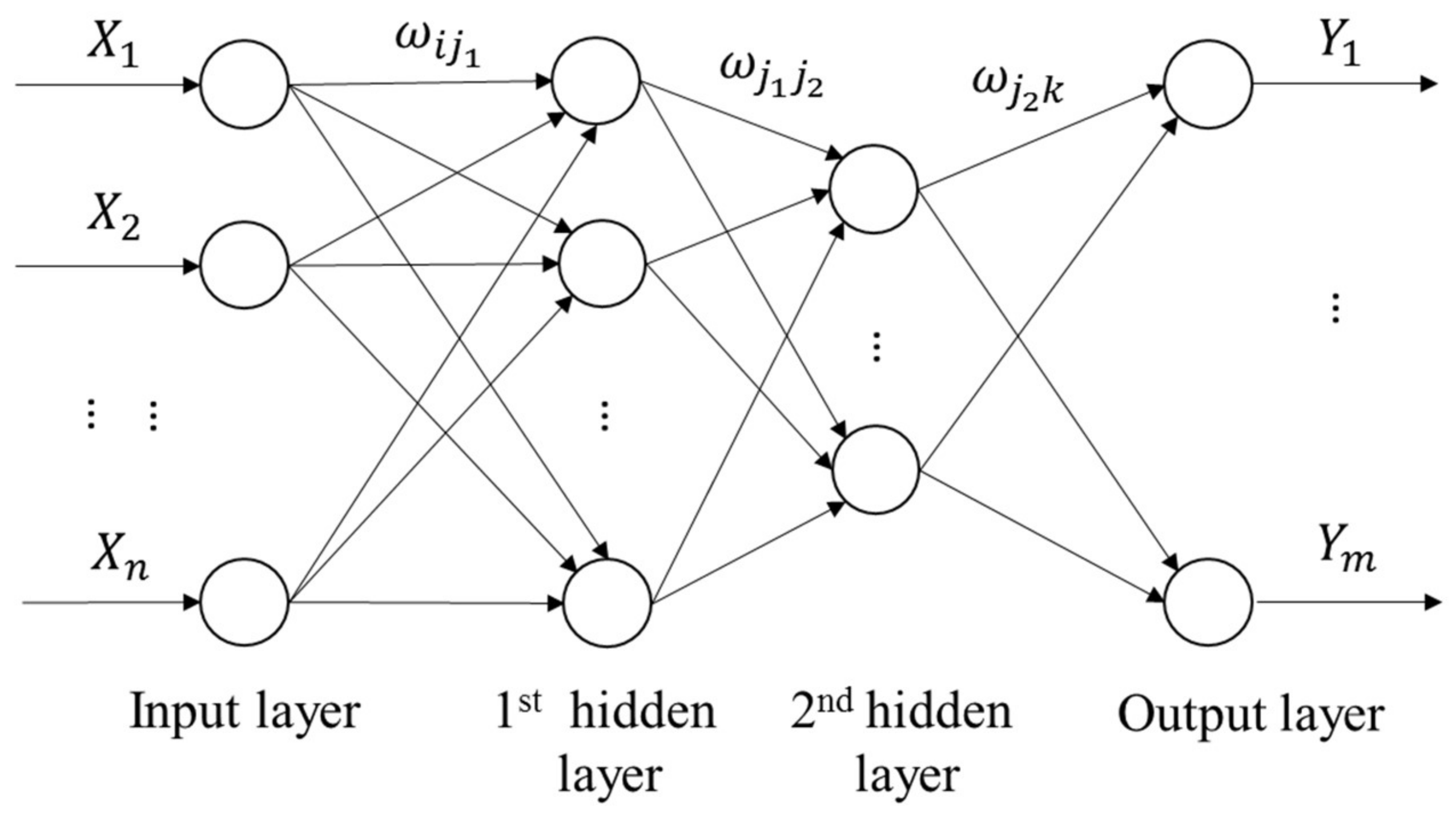
Figure 2.
Neural network’s training performance.

Figure 3.
Results of water resources demand in Wuxi by ANN.

Figure 4.
Results of energy demand in Wuxi by ANN.
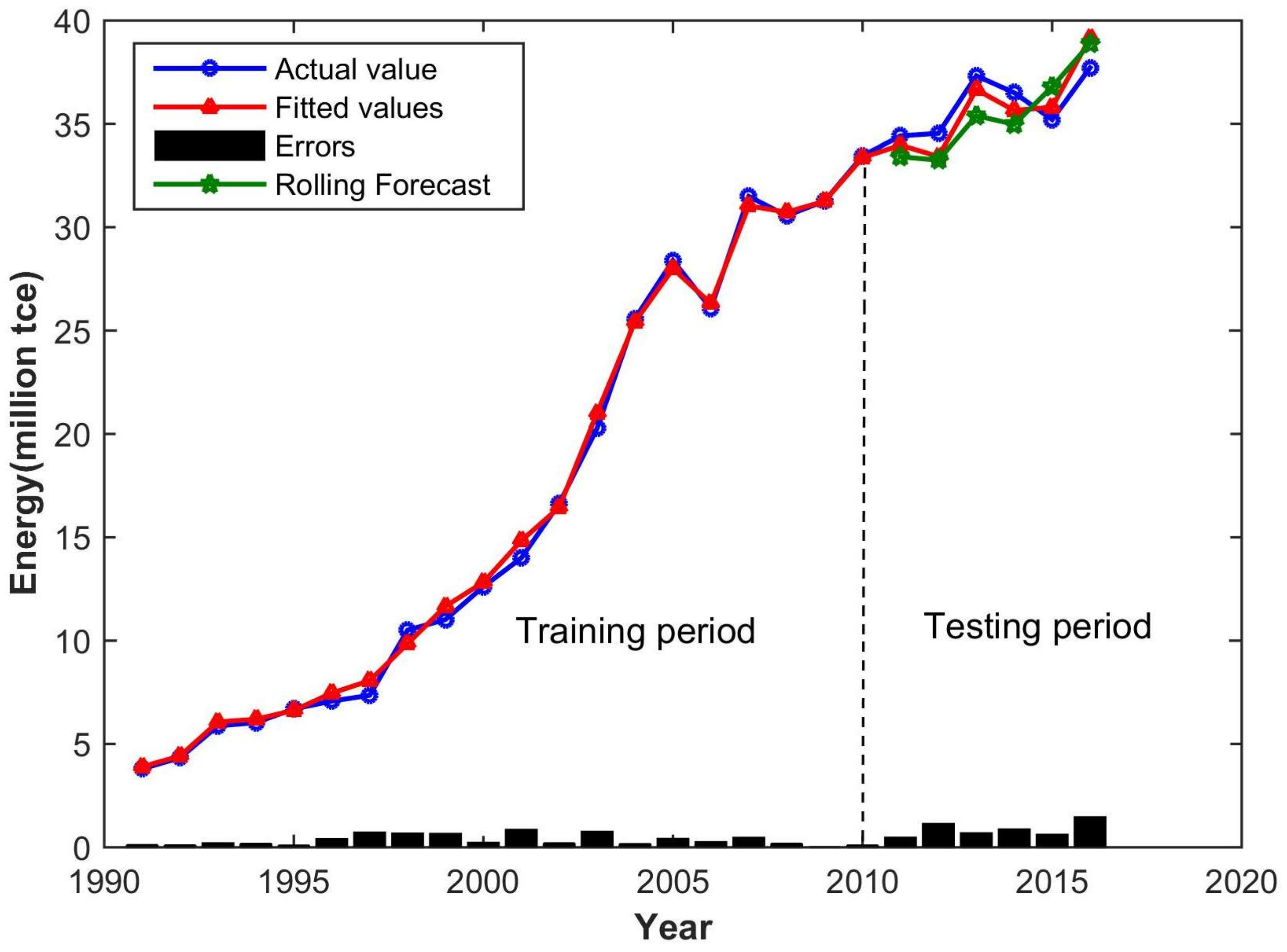
Figure 5.
MLR fitting results for water demand.
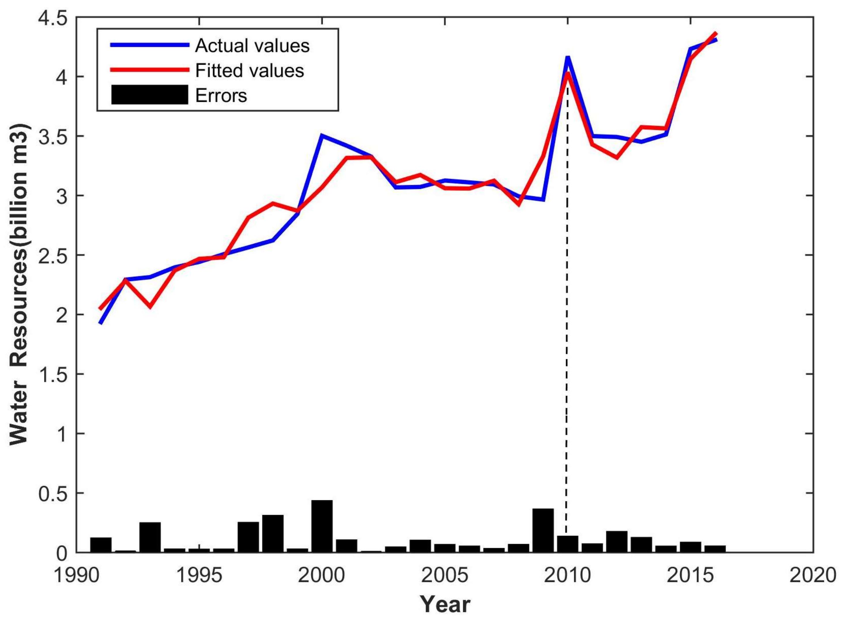
Figure 6.
MLR fitting results for energy demand.

Table 1.
Forecasted data of indices for water and energy demand in Wuxi in 2020 and 2030.
| Year | Total nt Population (X1)/Million people | Urban Population (X2)/Million people | Primary Industry GDP (X3)/Billion yuan | Secondary Industry GDP (X4)/Billion yuan | Tertiary Industry GDP (X5)/Billion yuan | Annual Precipitation (X6)/mm | Agricultural Water Consumption (X7)/Billion m3 |
| 2020 | 7.20 | 5.54 | 15.00 | 491.48 | 675.12 | 1387.5 | 0.94 |
| 2030 | 8.50 | 6.63 | 17.81 | 668.14 | 1644.88 | 1193.5 | 1.09 |
| Year | Industrial Water Consumption (X8)/Billion m3 | Tap Water Supply (X9)/Billion m3 | Total Discharge of Industrial Wastewater (X10)/Billion m3 | Daily Sewage Treatment Capacity (X11)/Million t | Consumption of Coal in Industrial Enterprises above the Designed Size (X12)/Million tce | Total Electricity Consumption (X13)/Billion kWh | Domestic Electricity Consumption (X14)/Billion kWh |
| 2020 | 3.46 | 0.39 | 0.21 | 1.54 | 25.00 | 803.22 | 6.39 |
| 2030 | 4.38 | 0.47 | 0.16 | 2.11 | 28.00 | 1042.81 | 7.60 |
Note: GDP = gross domestic product, tce = ton standard coal equivalent.
Table 2.
ANN Forecast of the water-energy demand for Wuxi.
| Year | Water Resources Demand/Billion m3 | Energy Demand/Million tce |
|---|---|---|
| 2020 | 4.843 | 47.561 |
| 2030 | 5.887 | 60.355 |
Table 3.
Regression coefficients of the multiple linear regression (MLR) models.
| Regression Coefficient | Estimated Values of Coefficients in Water Model | Estimated Values of Coefficients in Energy Model |
|---|---|---|
| β0 | 2.05901 | 13.60573 |
| β1 | 0.00320 | −0.02404 |
| β2 | −0.00670 | 0.01653 |
| β3 | 0.01728 | 0.00152 |
| β4 | −0.00177 | −0.00590 |
| β5 | 0.00024 | 0.00680 |
| β6 | −0.00018 | −0.00148 |
| β7 | −0.02755 | −0.12851 |
| β8 | 0.11397 | 0.27329 |
| β9 | −0.28824 | −0.40564 |
| β10 | −0.08571 | 0.06477 |
| β11 | 0.01214 | 0.01447 |
| β12 | 0.00044 | 0.01851 |
| β13 | 0.00455 | −0.02893 |
| β14 | 0.01092 | −0.05302 |
Table 4.
MLR Forecast results of water-energy demand for Wuxi.
| Year | Water Resources Demand/Billion m3 | Energy Demand/Million tce |
|---|---|---|
| 2020 | 5.661 | 49.188 |
| 2030 | 6.355 | 58.906 |
Table 5.
Comparison of the two models. MRE = mean relative errors.
| Model | Fitting Results | ||
|---|---|---|---|
| MRE of Water (%) | MRE of Energy (%) | Average of MRE (%) | |
| ANN | 1.58 | 2.71 | 2.14 |
| MLR | 3.88 | 2.84 | 3.96 |
© 2018 by the authors. Licensee MDPI, Basel, Switzerland. This article is an open access article distributed under the terms and conditions of the Creative Commons Attribution (CC BY) license (http://creativecommons.org/licenses/by/4.0/).
Share and Cite
MDPI and ACS Style
Yin, Z.; Jia, B.; Wu, S.; Dai, J.; Tang, D. Comprehensive Forecast of Urban Water-Energy Demand Based on a Neural Network Model. Water 2018, 10, 385. https://doi.org/10.3390/w10040385
AMA Style
Yin Z, Jia B, Wu S, Dai J, Tang D. Comprehensive Forecast of Urban Water-Energy Demand Based on a Neural Network Model. Water. 2018; 10(4):385. https://doi.org/10.3390/w10040385
Chicago/Turabian StyleYin, Ziyi, Benyou Jia, Shiqiang Wu, Jiangyu Dai, and Deshan Tang. 2018. "Comprehensive Forecast of Urban Water-Energy Demand Based on a Neural Network Model" Water 10, no. 4: 385. https://doi.org/10.3390/w10040385
Note that from the first issue of 2016, this journal uses article numbers instead of page numbers. See further details here.