High Resolution Monitoring of River Bluff Erosion Reveals Failure Mechanisms and Geomorphically Effective Flows


Department of Watershed Sciences, Utah State University, Logan, UT 84322-5210, USA
*
Author to whom correspondence should be addressed.
Water 2018, 10(4), 394; https://doi.org/10.3390/w10040394
Submission received: 22 February 2018
/
Revised: 20 March 2018
/
Accepted: 23 March 2018
/
Published: 28 March 2018
(This article belongs to the Special Issue Watershed Hydrology, Erosion and Sediment Transport Processes
)
Abstract
:Using a combination of Structure from Motion and time lapse photogrammetry, we document rapid river bluff erosion occurring in the Greater Blue Earth River (GBER) basin, a muddy tributary to the sediment-impaired Minnesota River in south central Minnesota. Our datasets elucidated dominant bluff failure mechanisms and rates of bluff retreat in a transient system responding to ongoing streamflow increases and glacial legacy impacts. Specifically, we document the importance of fluvial scour, freeze–thaw, as well as other drivers of bluff erosion. We find that even small flows, a mere 30% of the two-year recurrence interval flow, are capable of causing bluff erosion. During our study period (2014–2017), the most erosion was associated with two large flood events with 13- and 25-year return periods. However, based on the frequency of floods and magnitude of bluff face erosion associated with floods over the last 78 years, the 1.2-year return interval flood has likely accomplished the most cumulative erosion, and is thus more geomorphically effective than larger magnitude floods. Flows in the GBER basin are nonstationary, increasing across the full range of return intervals. We find that management implications differ considerably depending on whether the bluff erosion-runoff power law exponent, γ, is greater than, equal to, or less than 1. Previous research has recommended installation of water retention sites in tributaries to the Minnesota River in order to reduce flows and sediment loading from river bluffs. Our findings support the notion that water retention would be an effective practice to reduce sediment loading and highlight the importance of managing for both runoff frequency and magnitude.
1. Introduction
Humans have profoundly changed water and sediment fluxes in rivers worldwide [1,2,3,4,5,6,7]. Fluxes of fine sediment (clay, silt and fine sand) in particular have been directly affected by dam construction, urbanization, agriculture, fire suppression, mining, dredging, and logging [6]. Pervasive changes in watershed hydrology, due to anthropogenic climate change as well as land and water management actions, have indirectly amplified and damped sediment loading [8,9,10,11]. Such alterations in riverine fine sediment fluxes have important implications for channel and floodplain morphology [12,13], nutrient and contaminant transport [14,15,16], and aquatic habitat [17,18].
Problems of excess sediment and phosphorous affect a growing number of lakes and rivers globally, especially in agricultural landscapes [19]. Currently, 15% of all river miles in the USA are impaired by excess sediment [20]. Thus, effective strategies for reducing sediment loads are greatly needed. In order to develop effective sediment reduction strategies, it is essential to identify the sediment sources and factors causing excessive erosion [21]. Pinpointing the cause of excessive sediment loading is often complicated by the immense variability of climate and land use in both time and space, thresholds and nonlinear processes governing erosion, transport and deposition throughout a landscape, and a severe lack of sediment monitoring data, especially at small spatial scales [22]. Multiple, independent lines of information are often needed to properly constrain a sediment budget or watershed hydro-erosion model, in order to inform policy and management actions [7,23].
The Minnesota River basin (MRB) has been identified as a dominant contributor to sediment impairments in the Upper Mississippi River basin [24,25,26]. Ambitious sediment and nutrient reduction targets have been established for the MRB [27]. Thus, a suite of conservation measures are currently being considered to reduce sediment loading [28]. The hydroclimate of south central Minnesota, like large swaths of the Midwest, is becoming wetter and ongoing increases in artificial agricultural drainage continue to increase river runoff [10,11], creating more erosive flows.
Several studies document strong coupling between discharge and erosion of near-channel sediment sources (NCSS), such as streambanks and bluffs, at broad spatial (103+ km2) and temporal (semiannual to decadal) scales in the Minnesota River basin [7,9,10,29,30,31]. However, mechanistic linkages between NCSS erosion and streamflows have received less attention at finer spatial (101–102 m2) and temporal (daily to seasonal) scales. If sediment loading from NCSS is to be reduced in an effort to meet regional sediment reduction goals [27], then we need to better understand when and how these sources erode [21] in response to external drivers such as temperature, precipitation, and streamflow, all of which are changing due to shifts in climate and land use.
River bluffs are the dominant features contributing sediment in the Le Sueur River basin, which is the sub-basin of the MRB with the highest flow-weighted sediment loads [7,32]. Thus, reducing bluff erosion is essential for reducing sediment loading and improving water quality. Using repeat Terrestrial Laser Scanner (TLS) surveys, Day et al. (2013) measured higher annual bluff retreat rates when surveys bracketed larger magnitude flood events [33]. We build on these findings by answering several important questions: (1) Which physical processes accomplish the most bluff erosion? (2) Is there a threshold flow magnitude required to erode bluffs? and (3) Considering tradeoffs between frequency and magnitude of erosional events [34], what is the most geomorphically effective flow for bluff erosion? In an effort to inform sediment reduction strategies for the MRB [27,28] we present direct observations and high resolution measurements of river bluff erosion, the results of which allowed us to identify dominant failure mechanisms and geomorphically effective flows.
2. Methods
2.1. Study Sites
The 9200 km2 Greater Blue Earth River (GBER) watershed is a geomorphically transient basin with flat agricultural uplands and deeply incised river valleys in the lower portions of the watershed (Figure 1). The GBER is a major tributary to the MRB and is underlain by 15–100 m [35] of easily erodible glacial till, weakly lithified sandstones, and lacustrine deposits. The Blue Earth River and tributaries, including the Watonwan, Maple, Cobb, and Le Sueur rivers, erode tall (3–70 m) bluffs and terraces within the actively incising “knickzone”, the upper extent of which is marked by the green line in Figure 1. River and ravine incision began approximately 13,400 cal BP following paleo-flooding of Glacial River Warren (the modern-day Minnesota River) and continues at present [36,37]. Though riverine bluffs have dominated watershed sediment budgets in this basin since the end of the Pleistocene, erosion of bluffs has been further exacerbated by exceptionally high flows over the past few decades [7,21,38].
We monitored bluff erosion at 20 sites: 3 along the Blue Earth River, 7 along the Maple River, and 10 along the Le Sueur River (Figure 1). Surface areas are provided for all sites in Appendix A. Sites were selected to include a range of slope aspects and various material types (Appendix A, Table A1); priority was given to sites previously monitored by Day et al. 2013a and landowner access was required in all cases, as sites were located on private lands. See Appendix A Table A1 for site descriptions.
2.2. Data Aquisition
2.2.1. Daily Time Lapse Photographs
In June 2013, we installed six Canon PowerShot SX110 IS cameras (Canon Inc., Tokyo, Japan) in weatherproof cases, three each at sites LS9 and LS10. These cameras took one bluff photo per day and ran off of a solar panel configuration in summer, and an air alkaline battery configuration in winter. In early June 2015, we installed less expensive Cabela’s Outfitter 12MP IR HD Trail Cameras (Cabelas Inc., Sidney, NE, USA) at all 20 sites. Each camera, powered year-round by eight AA batteries, took a photo every three hours, recording photo time, date, and air temperature. Both types of cameras required manual data downloading.
2.2.2. Repeat Topographic Surveys using Structure-from-Motion Photogrammetry
We conducted 7 repeat photo surveys at each of two sites (LS9 and LS10) between June 2014 and May 2017 (Table 1). During each site visit we obtained 46–110 photographs from the bank opposite each bluff using a Panasonic Lumix® DMC-TS4 12.1 megapixel digital camera. Our image acquisition techniques in the field were consistent with Structure-from-Motion with Multi-View Stereo (SfM-MVS) guidelines outlined by [39]. Based on average point cloud density (1.25 pts/cm2), ground control root-mean-square error (0.027 m), as well as SfM–MVS post-processing time (30 h/survey for automated steps, and 10+ h/survey for manual steps), we found surveys containing ~100 photos were most effective for bluff surveys, each of which covered approximately 2500 m2.
Image acquisition surveys were conducted within several hours (up to 24 h) of total station ground control surveys, using a Leica TPS 1200. Prior to each bluff photo survey we installed 9 to 13 ground control points (GCPs)—pieces of rebar (0.95 cm diameter; 61 cm length), each with a 5.8 cm diameter orange cap. We surveyed the center location of each rebar cap using the total station in reflectorless mode to avoid rodman error and risk of injury. Total station survey closing error was <1 cm. Permanent benchmarks could not be established on either bank due to frequent, large erosion and/or deposition events. Therefore, new total station benchmarks were established at the start of each survey with coordinates obtained using a Leica CS15 and GS15 rtkGPS. GPS coordinates were obtained in real time while referencing the Minnesota Department of Transportation Continuously Operating Reference Network, typically achieving ±2–3 cm horizontal accuracy, and ±4–5 cm vertical accuracy. Easting and Northing coordinates reference NAD83 UTM Zone 15N and elevation coordinates reference NAVD88 ellipsoid heights.
2.3. Data Analysis
2.3.1. Inventory and Classification of Bluff Erosion Events
For each site we manually viewed daily photographs, deleting blurry and obstructed images. On average, 89% of days contained useable images; Table A1 in the Appendix A reports the percent of days with photographs for each site. In total we kept 12,608 images, all of which can be accessed with other raw data in the Supplementary Materials. For each day between 8 June 2015 and 15 May 2017 we indicated whether a photo existed and whether a large or small failure had occurred, based on repeat visual inspection by both an undergraduate researcher and S. Kelly. Daily photographs at site LS9 and LS10 extend back to June 2013, though the photo collection prior to May 2015 is less complete. The distinction between large and small failures was made based on size of the affected area, with large failures being those that exceeded 1 m2. The largest failures were further classified as either face or toe erosion events. Face erosion events occurred sub-aerially via mass wasting, block fall, slumping, or cantilever failure, primarily affecting in-situ till and/or Holocene terrace alluvium that caps the bluff. By contrast, toe erosion events coincided with high flow events, often removed failed colluvium, and occasionally eroded in situ till at the base of the bluff via fluvial abrasion or scour (Figure 1). For the 347 largest events, we classified whether failures were caused (based on photograph interpretations) by precipitation, freeze–thaw, sapping, rising limb flows, falling limb flows, ice breakup floods, structural instabilities (from previous failures), a combination of causes, or an unknown cause. Additionally, we categorically documented the duration of time that failed face material persisted at the toe of the bluff: one day to one week; one week to one month; one month to six months; six months to one year; and greater than one year.
2.3.2. Measuring Bluff Erosion using Structure-from-Motion Photogrammetry
We post-processed field-collected photo surveys using Agisoft PhotoScan Professional following best-practice methods outlined by [39,40,41,42]. For each survey we imported all non-blurry images; created photo masks; grouped photos by cameras based on focal length; aligned potos to create a sparse cloud, key point limit 100,000 and tie point limit 0; semiautomatically removed noisy points from sparse point clouds using gradual selection with a reconstruction uncertainty of 100; optimized cameras; manually removed noisy points, which were generally introduced from vegetation; reoptimized cameras; georeferenced point clouds using surveyed GCP coordinates; again reoptimized cameras; and finally reconstructed dense point clouds with ultra-high and mild depth filtering settings. Point clouds were manually edited for erroneous points (<10% of total points) usually introduced from vegetation, exported from PhotoScan as text files (.xyz), and then imported to CloudCompare to obtain bluff domain coordinates for point cloud rotations [43].
Bluff point clouds were built in real-world coordinates, however bluffs are near vertical features, often with overhangs, that erode in a direction normal to the bluff aspect and therefore perpendicular to the z coordinate axis. We rotated all point cloud coordinates using a MATLAB script (Appendix B) so that the measured direction of change in the z direction would capture erosion normal to the bluff aspect.
Once rotated, dense clouds were decimated to a 10 cm × 10 cm grid using the Topographic Analysis Toolkit (ToPCAT), developed by [44] and available from OpenTopography. This tool creates an output shapefile containing the mean, maximum, minimum, detrended standard deviation, as well as other statistics, associated with the subsampled point cloud. Subsampled points were computed using a minimum of four dense cloud points. Then we created 2.5-D rasters in ArcMap using the point to raster tool (10 cm grid) and differenced rasters using the Geomorphic Change Detection (GCD) tool [45]. Although terrestrial and aerial lidar surveys often build rasters using the zmin, or last returned/bare earth, elevation, Structure-from-motion does not necessarily provide bare earth elevations using zmin, especially in heavily vegetated areas. Error can occur all three dimensions; therefore we used zmean to build survey elevation rasters.
We constrained our final areal and volumetric change by probabilistically (99% CI) thresholding the DEM of difference (DoD) with a spatially propagated error surface generated for each survey. The error surface was created from the survey point cloud detrended standard deviation, or roughness, and the GCD defined SfM surveying uncertainty, 0.12 m. Where roughness was greater than 0.12 m, we assigned the roughness value to each error surface pixel, and where roughness was less than 0.12 m, we assigned the error surface pixel the value 0.12 m. Because we used the ground control points to georeference the dense point cloud, the GCP root-mean-squareerror (RMSE) reported in Table 1 is not an independent measure of point cloud accuracy. Therefore, we validated our topographic models using 9–20 checkpoints that were withheld from dense point cloud georeferencing and found an average survey RMSE of 0.11 m. Thus, it seems reasonable for a conservative assessment of change to assume 0.12 m as a minimum level of detection in areas of low roughness.
2.3.3. Estimating Bluff Erosion using Daily Photographs and Volume-Area Scaling Relation
Although repeat structure-from-motion photogrammetric surveys are relatively inexpensive, quick to acquire, and require minimal expertise to post-process using commercially available software packages, trade-offs exist between time spent in the field and lab and the overall accuracy of the survey [39,46]. Given that SfM surveys were not feasible at all 20 sites due to financial and time constraints, we developed a relation between bluff erosion volumes and areas based on SfM DoDs and repeat terrestrial laser scanner (TLS) surveys conducted by [33]. This allowed us to estimate bluff erosion volumes from digitizing areas of change for daily time lapse photographs. We find that mass wasting of riverine bluffs exhibit a power-law volume-area relation and compare the scaling exponent of our relation to the range of scaling exponents found for soil- and bedrock-cored landslides by [47,48,49,50] in Section 4.
Areas of change were manually digitized using the daily photographs for all of the large (>1 m2) erosional events. Depositional areas were excluded in order to measure face erosion and toe erosion separately, while minimizing the possibility of double-counting material. For large toe erosion events occurring over multiple days during a flood, we indicated small toe erosion events during the rising and falling limb flows and assigned the large toe erosion event to the date of the flood peak. Photographs from before and after each erosional event were imported to ArcMap 10.4 and erosional areas were digitized as shape files for the largest 347 events on record. For scale, we also digitized 1 to 4 orange rebar caps in each photograph. We used the average number of pixels per cap at each site and the measured rebar cap size () to estimate the average size of bluff failures (). Areas of bluff face erosion were converted to volumes of change using the previously described power-law, volume-area relation. Volumes of change were subsequently scaled by measured bluff area to calculate a spatially averaged (per 1 m × 1 m) bluff face retreat rate (m/day). Given the sum of all large events at each site we also calculated an average annual retreat rate for the period June 2015–May 2017.
We did not extrapolate bluff erosion volumes from areas of change for toe events because fluvial erosion of the toe occurs by a different set of processes (e.g., plucking, abrasion, dissolution), and volume-area scaling of toe erosion was poorly constrained in this study. Given that till erosion rates are likely set by rates of colluvium removal at the bluff toe, it is reasonable to assume that long-term average till and toe retreat rates are equal such that the bluff face slope retreats in parallel through time.
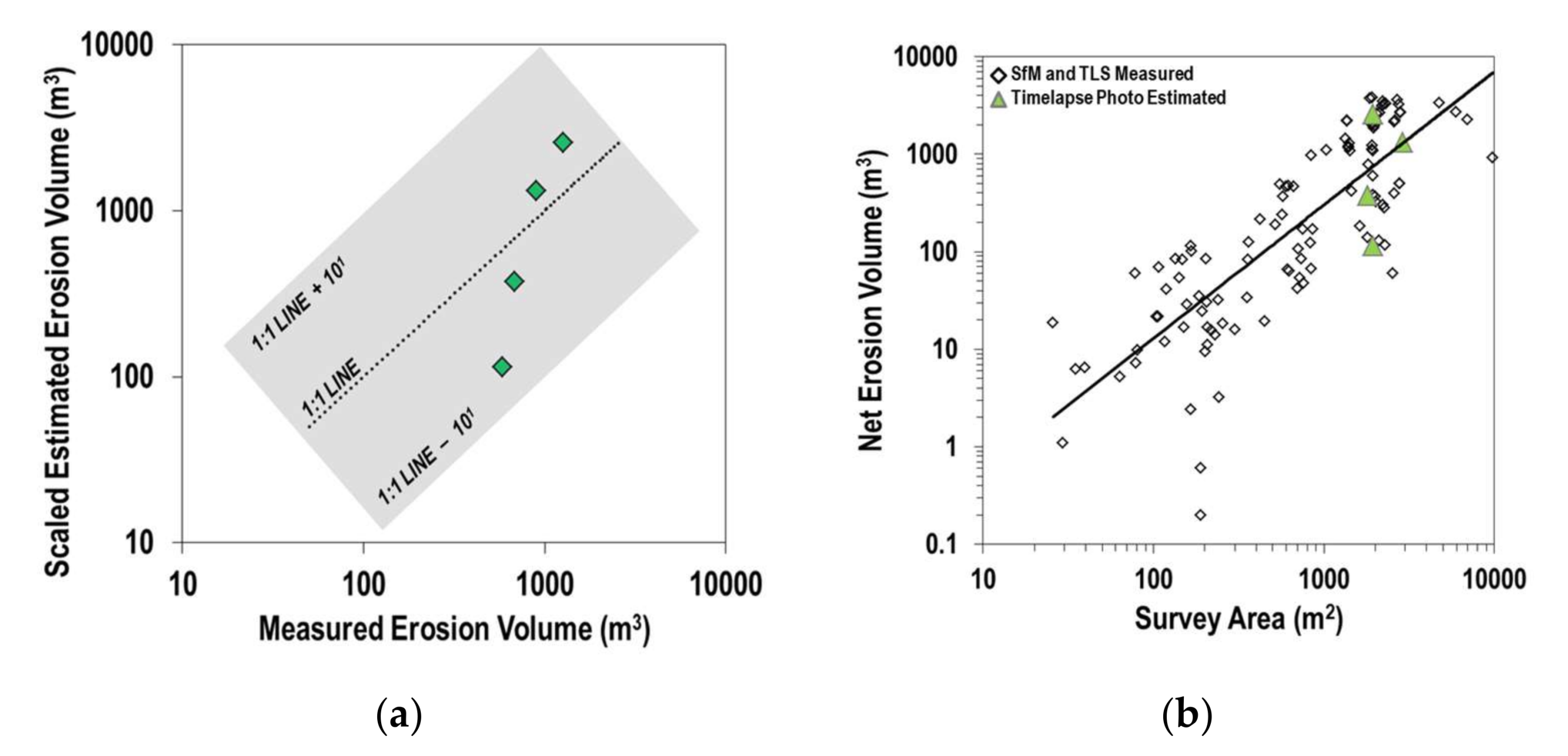
In Appendix A we present an assessment of the general accuracy of the volume-area scaling method for estimating bluff face erosion. Figure A1 compares measured areas and volumes of erosion from four SfM surveys at site LS10 that primarily capture bluff face erosion (6/15/2014–7/3/2014, 7/3/2014–5/9/2015, 5/9/2015–7/10/2015, and 10/22/2016–5/17/2017) to the sum of time lapse photo estimated face erosion for all events between SfM surveys.
2.3.4. Identifying Geomorphically Effective Flows
In order to identify geomorphically effective flows [34,51] for bluff retreat we calculated the exceedance probability and average runoff depth for mean daily flow values, then related daily flow values to each failure based on the failure observation date. For each bluff site, we calculated mean daily discharge exceedance probabilities based on a 10-year record: 1 October 2007–30 September 2017. For each site, we referenced the nearest streamflow gage on the respective river, as discussed in Appendix C. Appendix C also presents Log-Pearson III flood frequency analysis for a longer gage record, 1980–2016, for the Le Sueur River near Rapidan, MN (USGS 5320500) gage. Some results are discussed in relation to this gage in Section 4.
3. Results
Section 3.1 summarizes bluff failures observed in time lapse photos and discusses mechanisms of failure. Section 3.2 details measured bluff erosion volumes, retreat distances, and retreat rates obtained from repeat structure-from-motion surveys. The bluff erosion volume and area scaling relation is presented in Section 3.3. Finally Section 3.4 presents daily time lapse bluff erosion results in relation to river streamflow. Results identify geomorphically effective flows for bluff erosion, as well as minimum flows necessary for measureable toe erosion. Overall the results highlight the importance of streamflow and freeze–thaw processes, and furthermore indicate that bluff toe erosion occurs at flows much less than the “bankfull” flow that is typically considered the most geomorphically effective flow defining channel hydraulic geometry. Section 4 discusses these results in the context of using flow reductions to achieve sediment loading reductions in the Minnesota River Basin.
3.1. Daily Photographs Reveal Bluff Erosion Timing, Frequency, and Seasonal Failure Mechanisms
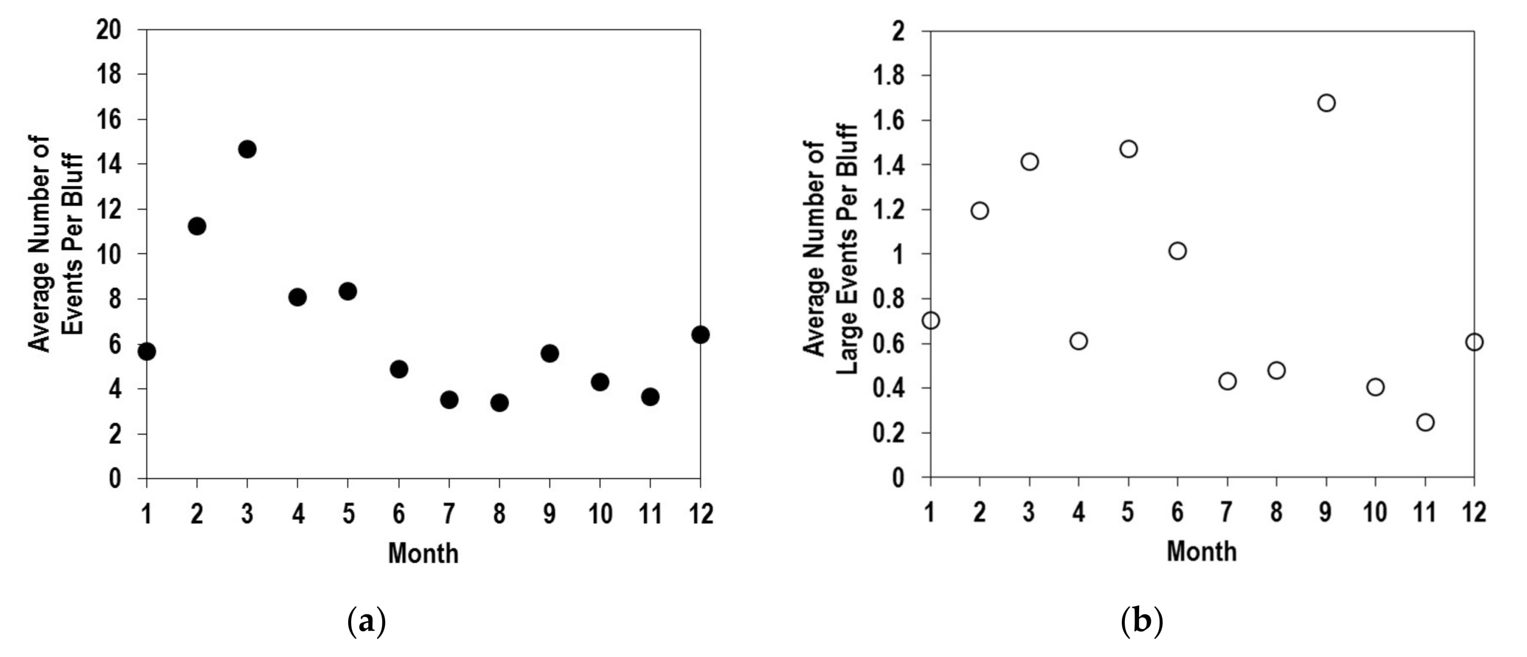
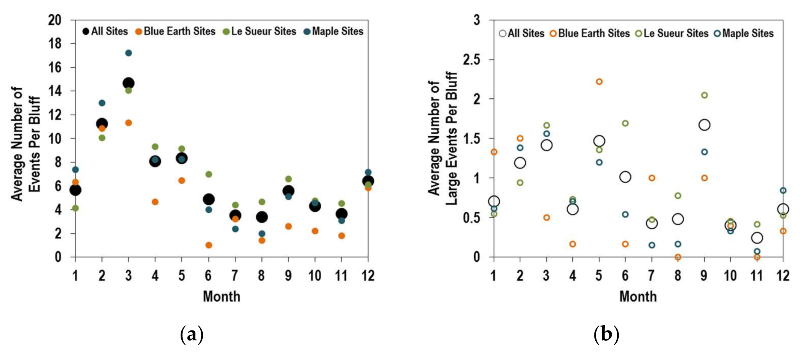
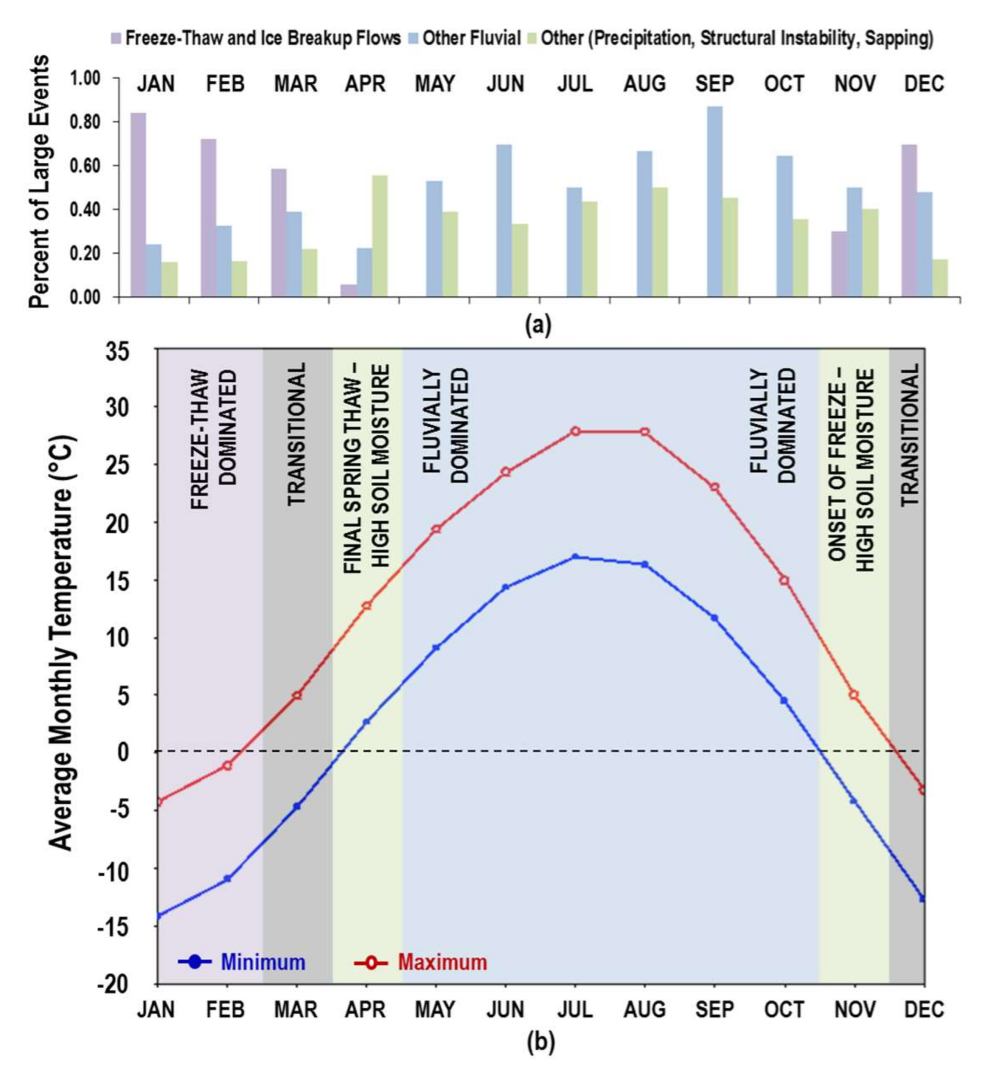
Between June 2015 and May 2017 we observed 2705 failures, of which 347 were classified as large (>1 m2). Of the 347 large events, 169 were large face events. Considering all failures, the greatest frequency of failures occurred in March when failures occur nearly half of all days (Figure 2a). Based only on frequency of occurrence, bluff failures peak seasonally during early spring months, February–May (Figure 2a), coinciding with diurnal freeze–thaw cycles, snowmelt and ice breakup floods, and late spring thaw driven by consecutive above-freezing temperature days.
The frequency of large failure events followed a different seasonal pattern compared with all failures (Figure 2a,b). For example, large failures were most frequently observed in September, not March. This result is explained almost entirely by a single extreme flood event (25-year return period) that occurred in late September 2016. The impact of this event is further discussed in Section 3.2 and Section 4. Large failures were also common in May and March, when many failures occur in both till and toe material as a result of seasonal spring thaw and snowmelt floods.
The overall pattern of seasonal bluff erosion frequency (Figure 2a,b) was consistent with individual patterns we observed for each of the three rivers on which we monitored bluffs (Appendix A, Figure A2). Slight differences among rivers, for example in the frequency of large events in September for the Le Sueur versus Blue Earth River, can be explained by local storm severity. Flood peaks were higher on the Le Sueur River than the Maple and Blue Earth rivers in September 2016 and consequently bluff erosion was more severe on the Le Sueur River bluffs [52].
Despite local variation in streamflow magnitudes and weather patterns, bluff erosion responded in a predictable manner to primary controls, such as normalized streamflow magnitudes (see Section 3.4) and aspect. We observed a significant positive regression relation between bluff aspect, measured in degrees from 180 degrees south, and the frequency of bluff failures for January (p = 0.0006, r2 = 0.49, F = 17.3) and February (p = 0.0037, r2 = 0.38, F = 11.1). During these months, generally northern facing bluffs remain snow-covered, while southern facing bluffs experience multiple snowfall and snowmelt events and frequent diurnal freeze thaw cycles based on interpretations from photographs and camera-recorded daytime and nighttime temperatures.
Interestingly, April (p = 0.0407, r2 = 0.24, F = 4.95) and November (p = 0.0289, r2 = 0.24, F = 5.64) exhibit weak, slightly significant negative regressions between bluff aspect and frequency of erosion, while March and December exhibit no significant relation (p > 0.05). It is likely that March and December are transitional months between winter and spring/fall. We did not observe any significant relation between bluff erosion frequency and aspect between May–October, likely because streamflow processes dominate erosion events and freeze–thaw is rare during these months. For further discussion of bluff erosion seasonality, see Appendix A, and Figure A3.
3.2. Structure-from-Motion Measured Bluff Erosion Volumes, Distances, and Rates
Figure 3 shows measured bluff erosion volumes and distances calculated from seven repeat structure-from-motion surveys at two monitoring sites, LS9 and LS10. For tabular results, reference Appendix A, Table A2. It should be noted that between our initial SfM survey in June 2014 and our final survey in May 2017, two major floods occurred. Based on Log-Pearson Type III analysis of peak flows (1980–2016) at the Le Sueur River gage near Rapidan, MN (USGS 5320500), downstream of all camera sites, the June 2014 and September 2016 floods were equivalent to 13- and 25-year recurrence interval floods, respectively (Appendix C). Not surprisingly, we measured the most volumetric change for surveys bracketing the September 2016 flood (2220–3510 m3 net erosion per site), which accounted for 74% (LS9) and 53% (LS10) of the total erosional change measured at each site over the three-year study period. Surveys bracketing the June 2014 flood captured the second largest net loss of material (~1080 m3 net erosion per site). In total, these two events accounted for 97% (LS9) and 79% (LS10) of the net erosion measured over the three-year study period.
June 2014 and September 2016 floods caused significant toe erosion at both sites (top left and bottom center panel in Figure 3a,b). Significant face erosion occurred at site LS10 during the June 2014 flood and at site LS9 during the September 2016 flood (Figure 3). To provide context for the size of these events, a local resident, who previously relocated her home due to erosion at site LS10, claims to have heard the failure and felt her house shake during the failure triggered on 18 June 2014. Three cameras installed on 4 in × 4 in × 8 ft fence posts buried 4-ft deep on the sand bar opposite bluff LS10 were disconnected from their power source and posts supporting the cameras were significantly slanted towards the floodplain, likely due to the transverse wave generated by the exceptionally large failure event (Figure 3). We previously observed a transverse wave at site LS10 following a considerably smaller face failure on 2 June 2014 (Supplementary Materials, Video S1).
Daily time lapse photos revealed that toe erosion caused by the June 2014 and September 2016 floods affected both colluvium and in situ till at the toe of all sites monitored. During, and following these large flood events, a clear pattern of significant face erosion (2–6 m, locally) and toe deposition (2–4 m, locally) was evident at site LS10 and to a lesser extent at site LS9 (Figure 3). Site LS9 has a large colluvial fan that has persisted along the bluff toe since 2010. Much of the erosion at site LS9 occurred along the bluff toe, especially on the upstream side of the colluvial fan (Figure 3a). During spring thaw, subdaily moving earthflows occurred on the upstream side of the colluvial toe (Figure 3a). At both sites, little erosion occurred between 12 July 2015 and 24 May 2016, a period of low flow. Based on daily time lapse photos, most of the change during this period occurred in March 2016, coinciding with spring thaw. Still, July 2015–May 2016 change was an order of magnitude less than the erosion associated with the June 2014 and September 2016 floods (Figure 3). Figure 3a shows that net deposition occurred on the bluff face at site LS9 between July 2015 and May 2016. Daily time lapse photos revealed erosion of upslope material at this site. Heavily forested, upslope areas were edited out of site LS9 SfM generated point clouds because dense vegetation introduces too much uncertainty to accurately measure change. Therefore, it is reasonable to end up with net deposition at site LS9 if sandy upslope material is eroded and deposited on the bluff colluvial toe.
By contrast, net deposition measured at site LS10 during relatively low flow period, October 2016 and May 2017, is likely due to differences in bulk density between in-situ till and toe colluvium (Figure 3b). Toe colluvium necessarily has a lower bulk density compared to in situ, overly consolidated till due to macropores between blocks of failed till. Additionally, the September 2016 flood undercut the bluff toe with irregularity, which may have left open spaces between the in situ till and the colluvial apron that could not feasibly be measured in the field. Both of these mechanisms would bias our GCD results in the direction of a small apparent volumetric gain despite conservation of mass. Day et al. 2013a found some sites with apparent net deposition between 2007 and 2009, when peak annual flows were modest (<2 year recurrence interval), though the cause of this apparent volumetric gain is not explicitly discussed.
Deposits of toe colluvium generally persist for short time periods (discussed in Section 3.4), and net erosion was predominant throughout the entire study period. Spatially averaged bluff retreat rates for sites LS9 and LS10 were 1.10 m/year and 1.28 m/year, respectively, per 1 m tall × 1 m along stream bluff surface area. Withholding the exceptionally high rates measured between 15 June 2014 and 3 July 2014 surveys, which bracket the 13-year recurrence interval flood by less than three weeks, measured annual rates are closer to 0.58 m/year. An even more conservative estimate, ignoring erosion caused by the September 2016 flood, puts average, quasi-background retreat rates at approximately 0.28 m/year. Given all survey SfM data collected between 2014 and 2017, sites LS9 and LS10 eroded on average 1.19 m/year.
3.3. SfM- and TLS-Derived Geometry Relations for Estimating Bluff Erosion from Daily Photographs
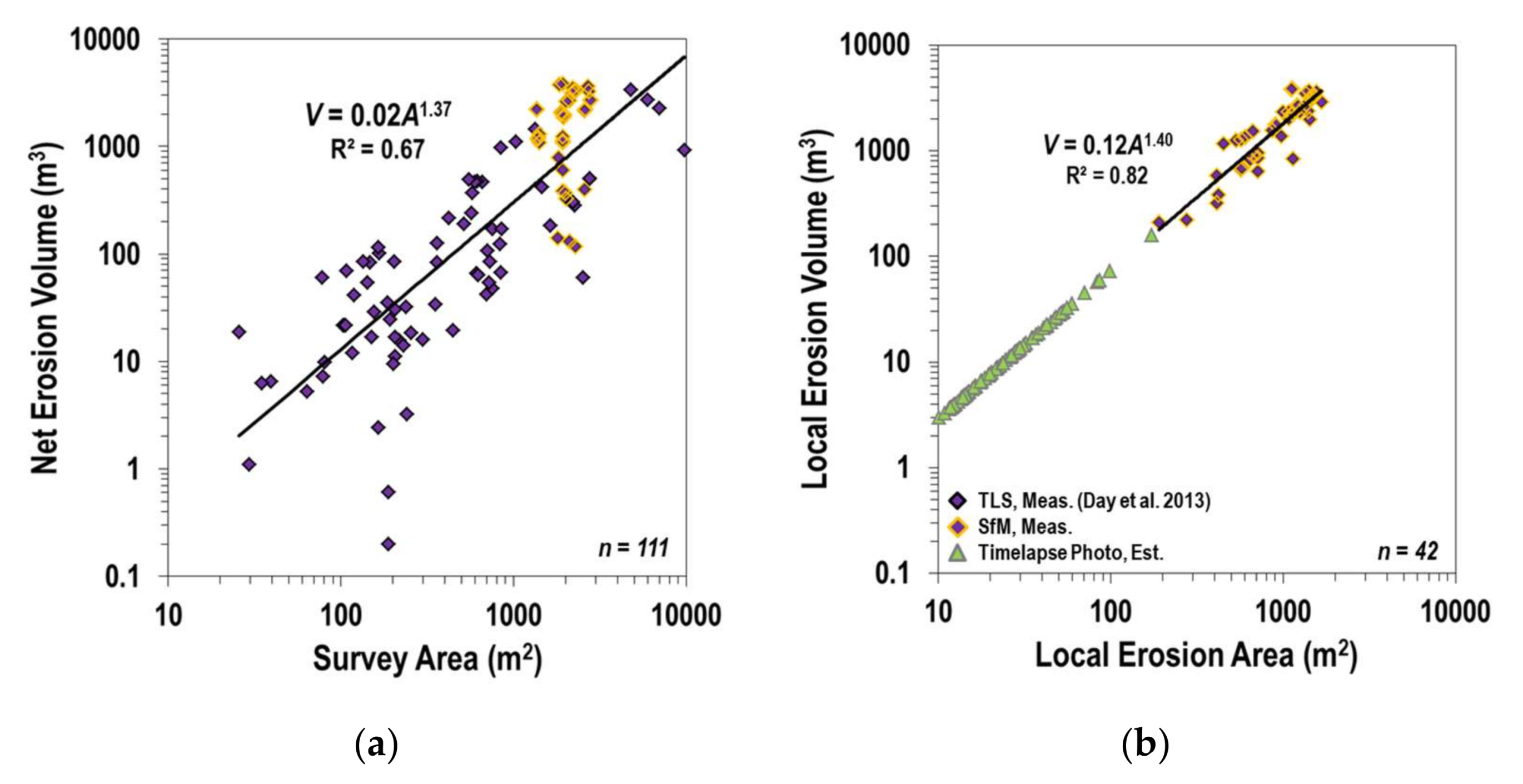
Based on SfM survey results (Appendix A, Table A2) and previously collected TLS surveys from Appendix A of Day et al. 2013a, we developed a bluff erosion volume-area power law scaling relation:
where the volume of the failure, V, is a function of the failure area, A, a scaling exponent, γ, and intercept, α. Figure 4 presents the volume-area relation between net survey erosion volume and bluff survey area using data from this study and Day et al. 2013a (Figure 4a) as well as between the locally measured erosion volume and area (i.e., the footprint of the failures themselves, Figure 4b). Day et al. 2013a only report net change and did not parse out erosion specifically in their results. Therefore, we did not want to assume that we could use the Day et al. 2013a data (Figure 4a) to create a volume-area scaling relation to convert our time lapse photo measurements of erosional areas to erosional volumes. Instead, we used the volume-area scaling relation constrained by our SfM measurements of erosion only, where γ = 1.4 and α = 0.12 (Figure 4b).
Although the scaling relations shown in Figure 4 were developed using different data sets, it turns out that both indicate a similar scaling exponent, γ, between 1.37–1.40. This is remarkable given that Figure 4a accounts for net erosion (erosion and deposition) and is spatially averaged across the entire bluff face and toe, while Figure 4b only accounts for areas of erosion of face material, or till. Similarity between gamma values suggests that deposition is essentially a negligible component of the overall signal, which is entirely consistent with our qualitative observations that erosion predominates bluff change. Virtually none of the sediment that eroded during our study was stored throughout the study period.
Observations at sites LS9 and LS10 covered a narrow range of areas, but fit well within the variability observed by Day et al. 2013a (Figure 4a). Thus, good agreement between the scaling exponents, regardless of the data used to build Figure 4a,b, suggests that we have likely covered enough local variability in erosion to apply the erosion scaling relation (Figure 4b) to areas of erosion measured from time lapse photos beyond sites LS9 and LS10. After scaling up the time lapse photo survey areas to those surveyed using SfM, there is reasonable agreement between SfM measured erosion and cumulative time lapse photo measured erosion for events that mostly affected the bluff face during SfM survey intervals (Appendix A, Figure A1). Estimated (from time lapse photos) and measured (from repeat SfM surveys) erosion rates are within the same order of magnitude. Further, estimated volumes are robust to digitization error (one standard deviation) of photo-estimated areas. Overall, we feel the scaling relation developed in this study is robust enough to estimate bluff erosion from areas of digitized erosion in order to determine the magnitude of geomorphically effective flows, presented in Section 3.4.
3.4. Geomorpically Effective Flows for Bluff Erosion
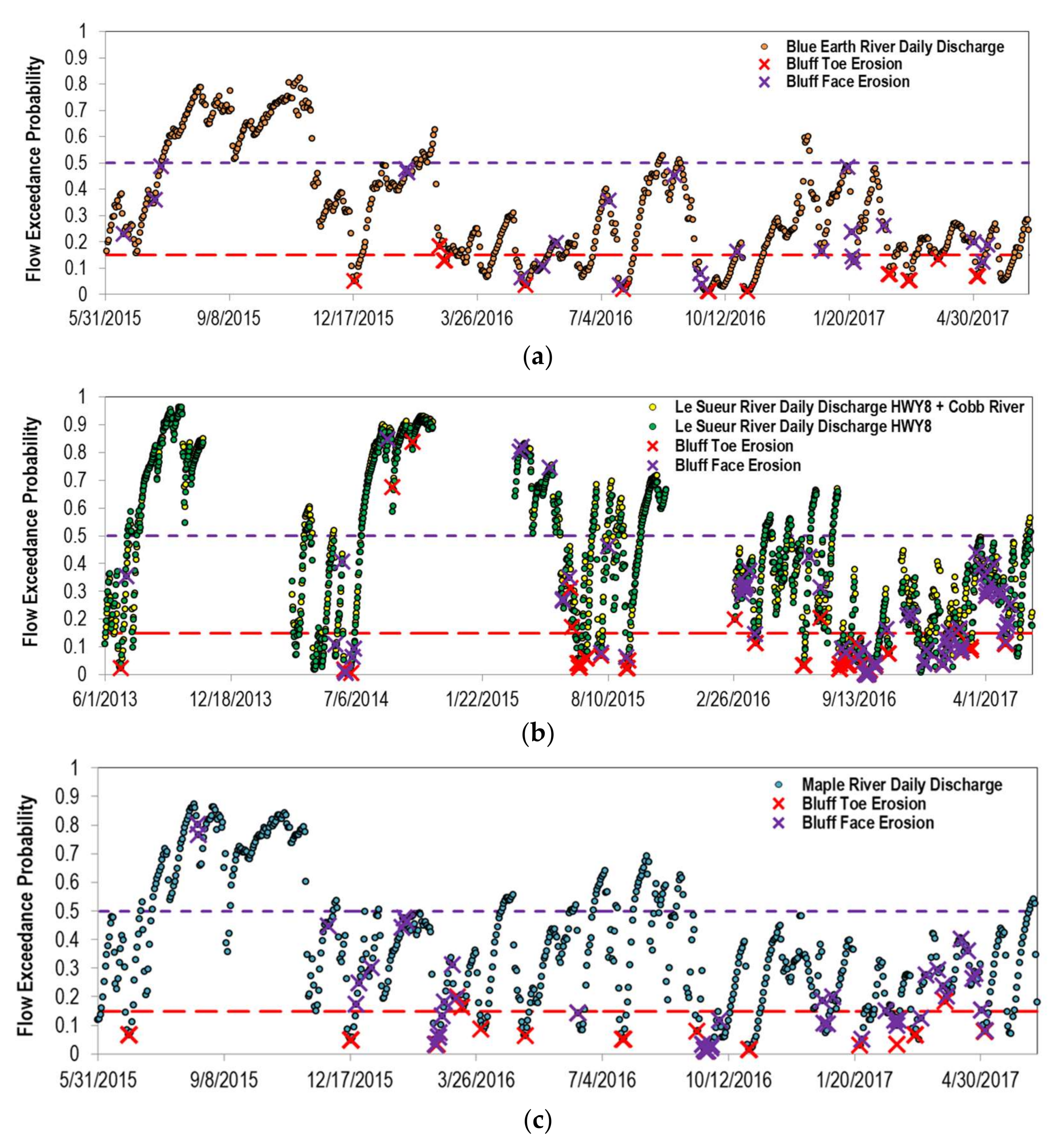
Due to the short timescale of this study (June 2015–May 2017) and the fact that we happened to capture an extreme flow event in September 2016, the erosion caused by the largest flood was much greater than anything measured in absence of this flood (Table A2). However, because an event of the magnitude of the 2016 flood occurs so infrequently (25-year return period), over long timescales, small floods (1–2 year return period) may in fact be more geomorphically effective. To begin to evaluate that hypothesis, we identified threshold flows for bluff toe and till erosion and examined the persistence of failed material.
Figure 5 shows the distribution of large bluff failures (separated by toe and face events) in relation to flow duration exceedance probabilities. There is a clear threshold for measureable (>1 m2) bluff toe erosion at 15% exceedance probability flows (1.3–2 mm/day of basin runoff). Not surprisingly, bluff face erosion has a much wider distribution because face erosion events, (a) may be directly related to oversteepening that occurs during toe erosion events, but are delayed in time, and (b) may be triggered by processes that are not directly related to streamflow, such as changes in matric suction or pore pressures as well as freeze thaw. That said, the fact that the vast majority of large face erosion events occur when flows are below 30% exceedance probability (>1 mm/day basin runoff) suggests that many face erosion events are triggered before, during, or after toe erosion events (Appendix A, Figure A4).
Based on the volume-area relation presented in Figure 4b, we calculated average bluff retreat rates (m/day) for face events and plotted retreat rates, event frequency, and total retreat against month (Figure 6a). Figure 6b shows large bluff failure frequency, event magnitude, and total retreat as a function of daily flow exceedance probabilities. Peaks in total retreat in March, June, and September in Figure 6a underscore the geomorphic importance of the September 2016 and June 2014 floods, as well as freeze–thaw, echoing the results of Section 3.2.
Daily photographs allowed us to differentiate between toe and face events. Therefore we could measure the persistence time of failed face material once it became toe alluvium. In general, face retreat rates measured at this daily or event timescale show greater retreat during lower exceedance probability flows (Figure 7a). This is especially true for events that persist for short amounts of time.
In general (95% of observations) face material does not persist as toe colluvium for longer than six months (Figure 7b). This is yet another line of evidence indicating that bluff erosion responds even to modest floods (less than 1 year recurrence interval). Face material that persists for the shortest amount of time (one day to one week) is generally small in size and/or coincides with larger flow events (Figure 7a,b).
Figure 7c also shows a positive power-law relation between bluff retreat rate and daily runoff depth (daily discharge volume normalized by basin area). This relation is stronger if we only include face events that occurred above a threshold discharge of 1 mm/day or <30% exceedance probability (Figure 7d), and stronger still when only examining the material that persisted from one day to one week (Figure 7e). Interestingly, the material that did not persist (i.e., failed face material that only persisted as toe material for very short periods of time), clusters at discharges near or above the 1 mm/day threshold.
Based on the power law relation between daily runoff depth (Q, mm/day) and time lapse photo estimated bluff erosion rate (E, m/day) developed in Figure 7d:
as well as the frequency of daily flow events, we calculated the magnitude × frequency product in order to identify geomorphically effective flows for the periods, June 2014–May 2017 and January 1940–December 2017 (Figure 8). Diamonds in Figure 8 indicate the product of magnitude and frequency with the large diamond representing the highest value computed. Several insights emerge from Figure 8.
Figure 8a suggests that the 1.3-year return period flow (1.9 mm/day) is the most geomorphically effective based on flow frequency and bluff erosion magnitude during the period 2014–2017. However, the flow frequency data is noisy during the short record, 2014–2017. The 1.2-year return interval flow (1.5 mm/day) produced on average 6.9 cm/year of erosion while the 1.3-year return interval flood accomplished on average 7.8 cm/year of bluff face erosion. These low flow magnitudes correspond well with the previously identified minimum measureable flows for bluff toe erosion, or 15% exceedance probability flows (equivalent to 1.5 mm/day at the Le Sueur River gage near Rapidan, MN (USGS 5320500).
The 1.2-year recurrence interval flood (1.5 mm/day) appears to have been the most geomorphically effective flood for bluff erosion in the Greater Blue Earth River basin during the period 1940–2017 (Figure 8b). The product of runoff event frequency and bluff erosion magnitude is mostly driven by event frequency, which mostly declines with increasing runoff. Bluff erosion magnitude increases, but at a slower rate when discharge increases according to the power law exponent 0.67. When event frequency is constant, the product follows the same nonlinear increase as the bluff erosion magnitude curve (Figure 8).
4. Discussion
4.1. Bluff Failure Timing, Frequency, and Seasonality
Based on frequency of events, March is an especially active time of year for bluff erosion, when bluffs erode nearly half of all days (Figure 2a). These events occur from a combination of subaerial and fluvial processes, including freeze–thaw and ice breakup floods (Figure A3). Overall, soil moisture is high and temperatures are transitioning towards mostly positive degree days (Figure A3). Despite major post-winter activity during spring thaw, events in March are generally small (Figure 2b and Figure 6a). Therefore, the greatest occurrence of large failures was in September (Figure 2b and Figure 6a), and the most total erosion occurred during September (Figure 6a). A 25-year recurrence interval flood occurred in September 2016. In absence of large floods, the relative importance of winter freeze–thaw and spring snowmelt on bluff erosion increases. These insights were made possible through an immense amount of manual digitization on time-lapse photographs. Given the value of this information, it would be beneficial for future studies to develop image-processing workflows to automate the process of identifying and quantifying failures.
4.2. Measured Bluff Erosion
Structure-from-motion measured bluff erosion rates (1.19 m/year) were much higher than those measured by Day et al. 2013a (0.20 m/year)–based on repeat TLS surveys (2007–2010) at 15 sites along the Le Sueur, Maple, and Big Cobb rivers. Day et al. 2013a measured bluff change immediately following a 12-year recurrence interval flood in March 2010. However, they captured that event at the end of their study period and therefore may have missed subsequent failures that occurred due to instabilities or oversteepening as a result of that event. In contrast, we captured a 13-year flood event at the beginning of our study period. Based on spatial patterns of bluff erosion at site LS10, extensive face erosion occurred during the two years following the June 2014 flood (Figure 3b). Had Day et al. 2013a continued to measure erosion in the years following the March 2010 flood, perhaps their bluff erosion rates would have been higher, as toe erosion caused by large floods seems to perpetuate erosion of the bluff face, even long after flood peaks have receded.
4.3. Generalizability of Our Volume-Area Scaling Relation
Measured bluff erosion exhibited a clear volume-area scaling relation and this relation was consistent between SfM and TLS [33] measured erosion, despite differences in areal extents and net erosion vs erosion and deposition (Figure 4a,b). Remarkably, an extensive analysis of 4231 individual landslide geometries conducted by Larsen et al. 2010 found γ = 1.1–1.3 for soil-based and γ = 1.3–1.6 for bedrock landslides, suggesting that γ is a property of the landslide material. The well consolidated till material in our study sites falls at the low end of bedrock in terms of mechanical properties, so an exponent of 1.4 is entirely consistent with the Larsen et al., 2010 scaling relation.
4.4. Geomorpically Effective Flows for Bluff Erosion
The Greater Blue Earth River basin makes up about 21% of the MRB watershed area and contains about 25% of the bluff surface area within the MRB (S. Day, unpublished data). Therefore reducing sediment loading in the GBER basin could have a substantial effect on sediment loading in the entire MRB. It is clear from our results that flow exerts a primary control on bluff erosion, with abrasion and scouring of the bluff toe causing oversteepening and eventual failure of the bluff face. Moderately high flows (1–2 mm/day) appear sufficiently capable of removing colluvial material deposited at the toe of the bluff. One of the primary sediment reduction strategies being considered in Minnesota involves reducing high flows via installation of water retention structures. Therefore, it is essential to understand which flows cause the most bluff erosion over time, considering both frequency and magnitude.
During our study period, the flow that caused the most erosion (based on SfM and time lapse photo results) was the September 2016, 25-year recurrence interval flood. Over long periods of time, this flood should be rare. At the lower end of geomorphically effective flows, we found flows less than 15% exceedance probabilities are effective at eroding bluff toe colluvium and in situ till. Fifteen percent exceedance probability is equivalent to 1–2 mm/day of runoff at each watershed outlet in the Greater Blue Earth River watershed. This flow threshold agrees well with a 1 mm/day threshold identified for erosion of near channel sediment sources by Cho [30].
We found that the 1.2-year recurrence interval flood should have been the most geomorphically effective flow during the period 1940–2017. However, the traditional Wolman and Miller type event frequency × response magnitude approach may underestimate the importance of very large events, which affect the geomorphic response long after the flood peak. To explore this idea further we discuss the sensitivity of the “geomorphically effective” flow to the erosion power law scaling relation exponent, γ.
Although it may seem reasonable to have identified the 1.2-year return interval flood as the most geomorphically effective flood during the period 1940–2017, it is harder to reconcile the 1.3-year flood being the most geomorphically effective during the period 2014–2017, given our daily time lapse and repeat SfM surveys. There are two reasons that likely explain why we found the 1.3-year return interval flood as the most geomorphically effective flow instead of the 13- or 25-year return interval floods. First, the 13- and 25-year floods also produce several days of lower magnitude flows, such as the 1.2- or 1.3-year flow, and very few days of substantially higher magnitude flows. Therefore, the impact of these events is diminished in a traditional Wolman and Miller style, magnitude-frequency approach. Second, the Q estimated bluff erosion approach likely underestimates the impact of large floods, as we only estimated bluff face erosion from time lapse photos and excluded bluff toe erosion, in volumetric terms, from our empirical data fit to Equation (2). Additional material removed during floods from fluvial scour and abrasion of glacial in situ till and failed colluvium below the water level is likely underestimating the impact of large flood events. Therefore, the exponent on the power-law relation presented in Figure 7d (0.67) may in fact be higher due to underestimated erosion totals during large floods. If the exponent is greater than 1, the importance of and implications for managing large food events become even greater.
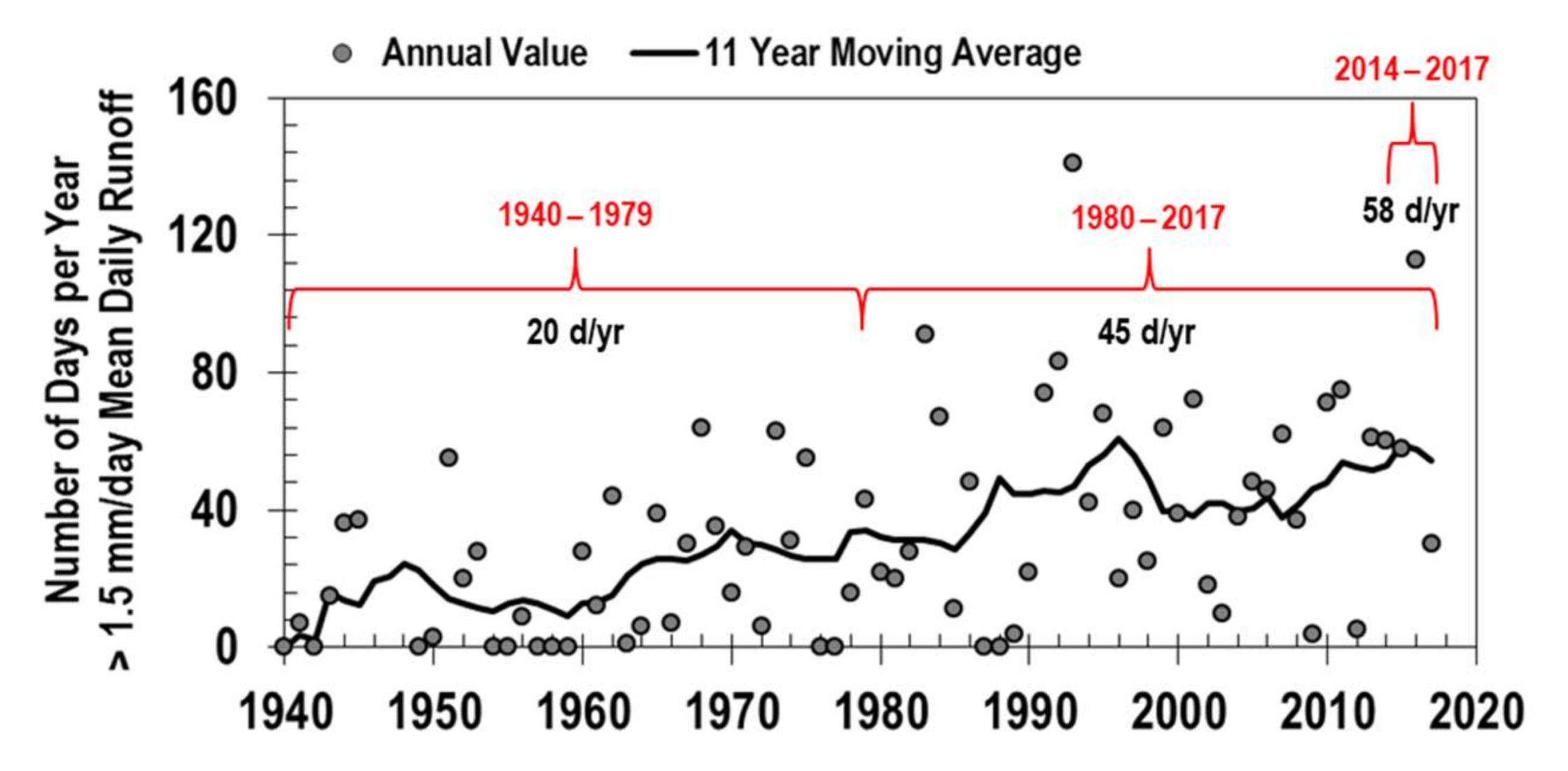
Using the magnitude of the 1.2-year recurrence interval flow (1980–2016) on the Le Sueur River near Rapidan, MN (USGS gage 5320500), we found the average occurrence (58 days/year) of this magnitude event during the period June 2014–May 2017 (Appendix C, Figure A6). By comparison, there were 20 and 45 days per year exceeding the 1.2-year return interval flood during the periods 1940–1979 and 1980–2017, respectively (Figure A6). In general, reducing the number of days each year with flows meeting or exceeding the 1.2-year recurrence interval flow should reduce annual loading from bluff erosion (Figure 8b). Future work should investigate tradeoffs between event frequency and magnitude, and additionally try to constrain bluff toe erosion as a function of discharge to inform sediment management strategies within the Minnesota River Basin.
5. Conclusions
Results of measured structure-from-motion photogrammetry and estimated time lapse photo bluff erosion rates lead us to several conclusions:
- Fluvial erosion was much more important than freeze–thaw and other subaerial processes during our study period, 2014–2017. The 13- and 25-year flood events caused 79–97% of the total erosion measured at two bluff sites on the Le Sueur River. Fluvial erosion is also the dominant long-term process driving bluff erosion, as toe colluvium must be removed by flows in order to continue bluff face erosion. In this way, the process of bluff erosion is very similar to landslide erosion, in which erosion rates are controlled by fluvial incision and uplift rates [47].
- Freeze–thaw and spring snowmelt influence bluff erosion rates between November and April. These processes exert greater influence on annual bluff erosion rates during low flow years. It is uncertain how climate change may amplify or dampen the importance of freeze–thaw processes in the Midwest USA, presenting opportunities for future researchers to expand upon frontiers in hillslope and fluvial geomorphology.
- Bluff erosion follows a power-law volume-area scaling relation with an exponent of 1.4, which is consistent with volume-area scaling found by Larsen et al. 2010 for landslides in weak bedrock [47].
- We captured two very large floods during a relatively short study period and thus measured 5.5× higher rates of annual bluff erosion than Day et al. 2013a and 2013b.
- Modest, 15% exceedance probability floods (30% of the 2-year recurrence interval flow), are capable of inducing bluff erosion.
- Considering only the relatively short period of time that we directly monitored bluff erosion, we found that the vast amount of geomorphic work was done by the 13- and 25-year recurrence interval flows.
- Using daily runoff frequency, estimated bluff face erosion magnitude, and their product as a function of daily runoff, the most “geomorphically effective” flow for bluff erosion from 1940 to 2017 was the 1.5 mm/day or 1.2-year recurrence interval flood. Coincidently, this is the minimum flow necessary for measureable toe erosion, though future work should better constrain bluff toe erosion as a function of discharge.
Several major tributaries of the Minnesota River basin are responding to human and climate driven flow increases, as well as glacial legacy impacts by increasing river width, which recruits fine sediment from till deposits along the river valley margin. Bluffs will continue to erode, even if current hydrologic conditions do not change, until the channel geometry comes into equilibrium with the flow regime. If geomorphically effective peak flow magnitudes and/or their occurrence continue to increase, as they have in many river basins of the Midwest, USA during the late 20th and early 21st centuries, then managing erosion of near channel sediment sources may only become more challenging in the future. Sediment-targeted management strategies in the Greater Blue Earth River basin and other MRB tributary basins should explicitly account for tradeoffs between streamflow timing, frequency, and magnitude, as well as the effects of freeze–thaw and flood events (which are often underrepresented) on overall bluff erosion under future human and climate scenarios.
Supplementary Materials
The following are available online at https://www.mdpi.com/2073-4441/10/4/394/s1, Video S1: Bluffs-Downstream-Camera B Timelapse.mp4, Video S2: Bluffs-Upstream-Camera A Timelapse.mp4, Video S3: bluff_failure.m4v, as well as all raw data, including all photos, SfM surveys, derivative files and spreadsheets used for analysis.
Acknowledgments
This material is based upon work supported by the Geological Society of America Graduate Student Research Grant, the National Science Foundation (NSF) Graduate Research Fellowship Program (Grant No. 1147384), the NSF Water Sustainability and Climate (WSC)—Category 2 grant (EAR-1209445). Authors thank Peter Wilcock, Jack Schmidt, Joe Wheaton, and Jiming Jin, as well as current and former members of the Belmont Hydrology and Fine Sediment Laboratory for discussions. Two anonymous reviewers provided useful feedback. We thank Brendan Murphy for writing a Matlab script for point cloud rotation (Appendix B). Additional gratitude is extended to Se Jong Cho, St. Anthony Falls Research Laboratory; Stephanie Day, North Dakota State University; Karen Gran, University of Minnesota, Duluth; Philip Larson, Ben Von Korff, and many Geography Department undergraduate and graduate students, Minnesota State University, Mankato; Andy Wickert University of Minnesota, Minneapolis; Efi Foufoula-Georgiou, University of California Irvine; and many Blue Earth County, MN landowners.
Author Contributions
Sara Kelly conceived the project idea, collected and analyzed data with help from Patrick Belmont and those listed in the acknowledgements, and wrote the manuscript. Patrick Belmont supervised the project and contributed to manuscript writing and revisions.
Conflicts of Interest
Patrick Belmont, a co-author, is the Guest Editor for the Water Special Issue: Watershed Hydrology, Erosion and Sediment Transport Processes but recused himself from the review process for this paper. Funding sources had no role in the design of the study; in the collection, analyses, or interpretation of data; in the writing of the manuscript, or in the decision to publish the results.
Appendix A

Table A1.
Time lapse camera site information. Easting and Northing coordinates reference datum NAD83, and projection UTM Zone 15N.
Table A1.
Time lapse camera site information. Easting and Northing coordinates reference datum NAD83, and projection UTM Zone 15N.
| Site Name 1 | Site Description 2 | Aspect (°) | Survey Dimensions L(m) × H(m) | Easting (m) | Northing (m) | Photo Dates | Days w/Photos (%) |
|---|---|---|---|---|---|---|---|
| BE1 | NC, TC, FA | 153 | 22 × 7 | 412,910 | 4,877,097 | 6/9/2015–5/16/2017 | 98 |
| BE2 | NC, IS, OC | 229 | 26 × 14 | 413,266 | 4,877,247 | 6/8/2015–5/16/2017 | 83 |
| BE3 | NC, IS, OC | 174 | 24 × 11 | 413,786 | 4,878,851 | 6/9/2015–5/16/2017 | 100 |
| MPL1 | NC, IS, OC | 274 | 20 × 10 | 414,108 | 4,870,395 | 6/4/2015–5/12/2017 | 94 |
| MPL2 | NC, IS, OC | 180 | 20 × 11 | 414,145 | 4,870,844 | 6/5/2015–5/12/2017 | 100 |
| MPL3 | OC | 193 | 22 × 9 | 415,540 | 4,873,137 | 6/7/2015–5/13/2017 | 99 |
| MPL4 | NC, TC, FA | 69 | 21 × 6 | 416,018 | 4,874,079 | 6/7/2015–5/13/2017 | 92 |
| MPL5 | NC, TC, FA | 116 | 17 × 6 | 415,988 | 4,874,321 | 6/8/2015–5/13/2017 | 100 |
| MPL6 | OC | 166 | 21 × 13 | 416,435 | 4,875,258 | 6/8/2015–3/16/2016 | 70 |
| MPL7 | OC, TC, IS | 170 | 20 × 14 | 418,051 | 4,878,666 | 6/8/2015–3/29/2017 | 99 |
| LS1 | OC | 292 | 18 × 7 | 424,457 | 4,884,466 | 5/22/2015–5/18/2017 | 80 |
| LS2 | NC, TC, FA | 228 | 23 × 12 | 424,533 | 4,884,155 | 7/11/2015–5/13/2017 | 95 |
| LS3 | NC, IS, OC | 118 | 23 × 17 | 423,608 | 4,883,232 | 6/7/2015–5/14/2017 | 91 |
| LS4 | NC, OC | 36 | 23 × 13 | 422,105 | 4,882,098 | 6/7/2015–5/14/2017 | 84 |
| LS5 | OC, TC, FA | 180 | 20 × 6 | 421,975 | 4,882,474 | 6/7/2015–5/13/2017 | 58 |
| LS6 | OC, TC, FA | 138 | 20 × 9 | 421,918 | 4,882,463 | 6/8/2015–5/14/2017 | 98 |
| LS7 | OC, TC, FA | 262 | 28 × 11 | 420,202 | 4,881,018 | 6/7/2015–5/13/2017 | 99 |
| LS8 | OC, TC, FA | 222 | 23 × 7 | 419,815 | 4,881,174 | 6/7/2015–3/10/2016 | 68 |
| LS9 | NC, IS | 70 | 21 × 20 | 418,666 | 4,881,123 | 6/3/2014–5/15/2017 | 82 |
| LS10 | OC, TC, FA | 270 | 21 × 16 | 419,186 | 4,881,486 | 6/2/2014–5/15/2017 | 93 |
1 Site names abbreviated for each river: Blue Earth River (BE), Maple River (MPL), and Le Sueur River (LS). Site numbers correspond to independent sites from upstream to downstream (1, 2, 3, …). 2 Site descriptions are reported as general stratigraphic units from bluff base to crest. Abbreviations correspond to the following: normally consolidated till (NC); overly consolidated till (OC), interglacial sands (IS), terrace channel alluvium (TC), floodplain alluvium (FA).
Table A2.
Geomorphic change detection results from repeat SfM surveys at two bluffs sites on the Le Sueur River. Average annual retreat rates calculated as net volume lost (erosion positive) divided by entire survey area, divided by the amount of time, in years, between surveys. Right two columns report results for areas of erosion only.
| Site Name | Survey 1 Date | Survey 2 Date | Survey Area (m2) | Net Volume Lost (m3) | Retreat Rate (m/year) | Erosion Area (m2) | Erosion Volume (m3) |
|---|---|---|---|---|---|---|---|
| LS9 | 6/15/2014 | 7/3/2014 | 1938.8 | 1082.0 | 11.3 | 451.0 | 1163.0 |
| LS9 | 6/15/2014 | 5/8/2015 | 1928.3 | 1229.0 | 0.71 | 538.0 | 1254.0 |
| LS9 | 6/15/2014 | 7/12/2015 | 1930.3 | 1132.6 | 0.55 | 604.0 | 1335.0 |
| LS9 | 6/15/2014 | 5/24/2016 | 1834.0 | 785.0 | 0.22 | 667.0 | 1524.0 |
| LS9 | 6/15/2014 | 10/22/2016 | 1931.6 | 3826.0 | 0.84 | 1129.0 | 3837.0 |
| LS9 | 6/15/2014 | 5/17/2017 | 1857.9 | 3759.0 | 0.69 | 1119.0 | 3785.0 |
| LS9 | 7/3/2014 | 5/8/2015 | 2111.3 | 131.2 | 0.07 | 191.0 | 207.0 |
| LS9 | 7/3/2014 | 7/12/2015 | 2297.2 | 117.2 | 0.05 | 424.0 | 381.0 |
| LS9 | 7/3/2014 | 5/24/2016 | 2138.7 | −224.1 | −0.06 | 716.0 | 841.0 |
| LS9 | 7/3/2014 | 10/22/2016 | 2318.4 | 3275.3 | 0.61 | 1533.0 | 3279.0 |
| LS9 | 7/3/2014 | 5/17/2017 | 2190.0 | 3117.3 | 0.50 | 1452.0 | 3146.0 |
| LS9 | 5/8/2015 | 7/12/2015 | 2157.2 | −113.0 | −0.29 | 276.0 | 221.0 |
| LS9 | 5/8/2015 | 5/24/2016 | 2037.8 | −481.6 | −0.23 | 576.0 | 655.0 |
| LS9 | 5/8/2015 | 10/22/2016 | 2130.4 | 2674.6 | 0.86 | 1217.0 | 2682.0 |
| LS9 | 5/8/2015 | 5/17/2017 | 2037.0 | 2597.7 | 0.65 | 1229.0 | 2626.0 |
| LS9 | 7/12/2015 | 5/24/2016 | 2385.2 | −355.0 | −0.17 | 646.0 | 817.0 |
| LS9 | 7/12/2015 | 10/22/2016 | 2713.6 | 3598.3 | 1.04 | 1562.0 | 3604.0 |
| LS9 | 7/12/2015 | 5/17/2017 | 2756.5 | 3256.9 | 0.64 | 1488.0 | 3292.0 |
| LS9 | 5/24/2016 | 10/22/2016 | 2227.2 | 3513.2 | 3.81 | 1419.0 | 3662.0 |
| LS9 | 5/24/2016 | 5/17/2017 | 2250.5 | 3240.0 | 1.47 | 1358.0 | 3462.0 |
| LS9 | 10/22/2016 | 5/17/2017 | 2616.1 | −324.6 | −0.22 | 412.0 | 316.0 |
| LS10 | 6/15/2014 | 7/3/2014 | 1420.6 | 1086.7 | 15.5 | 574.0 | 1270.0 |
| LS10 | 6/15/2014 | 5/9/2015 | 1396.9 | 1210.0 | 0.97 | 870.0 | 1551.0 |
| LS10 | 6/15/2014 | 7/10/2015 | 1410.9 | 1302.0 | 0.85 | 916.0 | 1729.0 |
| LS10 | 6/15/2014 | 5/24/2016 | 1390.9 | 1174.0 | 0.43 | 908.0 | 1751.0 |
| LS10 | 6/15/2014 | 10/22/2016 | 1372.1 | 2225.0 | 0.69 | 1140.0 | 2242.0 |
| LS10 | 6/15/2014 | 5/17/2017 | 1363.2 | 2182.0 | 0.55 | 1003.0 | 2291.0 |
| LS10 | 7/3/2014 | 5/9/2015 | 1807.6 | 139.9 | 0.09 | 582.0 | 686.0 |
| LS10 | 7/3/2014 | 7/10/2015 | 2021.3 | 325.0 | 0.16 | 1144.0 | 831.0 |
| LS10 | 7/3/2014 | 5/24/2016 | 2005.3 | 366.0 | 0.10 | 983.0 | 1365.0 |
| LS10 | 7/3/2014 | 10/22/2016 | 1984.9 | 1958.0 | 0.43 | 1436.0 | 1965.0 |
| LS10 | 7/3/2014 | 5/17/2017 | 1969.9 | 1857.0 | 0.33 | 1258.0 | 2329.0 |
| LS10 | 5/9/2015 | 7/10/2015 | 1947.7 | 380.3 | 1.08 | 414.0 | 582.0 |
| LS10 | 5/9/2015 | 5/24/2016 | 1941.6 | 599.0 | 0.30 | 718.0 | 949.0 |
| LS10 | 5/9/2015 | 10/22/2016 | 1915.8 | 2009.0 | 0.72 | 1085.0 | 2011.0 |
| LS10 | 5/9/2015 | 5/17/2017 | 1901.9 | 2070.0 | 0.55 | 1148.0 | 2237.0 |
| LS10 | 7/10/2015 | 5/24/2016 | 2587.2 | 396.7 | 0.18 | 719.0 | 628.0 |
| LS10 | 7/10/2015 | 10/22/2016 | 2807.7 | 2691.0 | 0.75 | 1371.0 | 2708.0 |
| LS10 | 7/10/2015 | 5/17/2017 | 2800.3 | 2650.0 | 0.51 | 1671.0 | 2852.0 |
| LS10 | 5/24/2016 | 10/22/2016 | 2607.7 | 2219.6 | 2.06 | 1082.0 | 2293.0 |
| LS10 | 5/24/2016 | 5/17/2017 | 2580.9 | 2127.0 | 0.84 | 1401.0 | 2340.0 |
| LS10 | 10/22/2016 | 5/17/2017 | 2890.8 | −130.3 | −0.08 | 673.0 | 895.0 |
Table A3.
Daily discharge (Q) estimated bluff erosion magnitude × observed Q (mm/day) frequency (right four columns)—estimated using different daily erosion-discharge power law scaling exponents, gamma—validated against measured retreat rates from Day et al. 2013a (D13a) and 2013b (D13b) and Kelly and Belmont, this paper (K&B) collected data.
| Survey Dates | Data, Authors/Source/Method | Measured, Retreat (m/year) ± 95% CI | Q (mm/day), est. Retreat (m/year), γ = 0.66 | Q (mm/ day), est. Retreat (m/year), γ = 0.67 | Q (mm/ day), est. Retreat (m/year), γ = 1.00 | Q (mm/day), est. Retreat (m/year), γ = 1.35 |
|---|---|---|---|---|---|---|
| January 1938–December 2005 | D13b/AP/Crest retreat | 0.14 ± 0.02 | 0.47 1 | 0.42 1 | 0.68 1 | 1.03 1 |
| July 2007–June 2010 | D13a/TLS/Site ero. | 0.20 ± 0.04 | 0.68 | 0.62 | 1.03 | 1.67 |
| June 2014–May 2017 | K&B/SfM/Site ero. | 1.19 ± 0.87 | 1.32 2 | 1.20 | 1.99 | 3.26 |
1 Q record available beginning 1940 and missing data 1945–1949. 2 Italicized values are estimated retreat rates. Underlined values fall with the 95% confidence interval of measured (nonitalicized) retreat rates.
Figure A1.
(a) Measured bluff erosion from four SfM surveys, 6/15/2014–7/3/2014, 7/3/2014–5/9/2015, 5/9/2015–7/10/2015, and 10/22/2016–5/17/2017, which primarily capture bluff face erosion vs the sum of time lapse photo estimated erosion, using the scaling relation, V = 0.12A1.4. (b) Bluff survey area vs net erosion volume for SfM and TLS measured surveys (black diamonds) and time lapse photo estimated areas and volumes (green triangles). Estimated erosion is within the same order of magnitude as SfM-measured erosion for the same time periods.

Figure A2.
(a) Average number of failure days per month for a bluff of average size 250 m2 (length × height). Average monthly days with failures are plotted for sites grouped by each river and for all bluff sites. Total number of observations: 2705 events; (b) average number days with large failures per month for sites grouped by each river and for all bluff sites. Number of observations: 347 events.

Figure A3.
(a) Percent of large events likely triggered by freeze–thaw and ice breakup floods (purple), other ice-free floods (blue), and other processes including precipitation, structural instability, and seepage/sapping (green), based on qualitative photographic interpretations. Total number of observations: 347 events. Monthly percentages do not sum to 1 because some events were triggered by multiple processes and for some events, the cause of failure could not be determined; (b) average monthly maximum (red) and minimum (blue) temperatures based on long term mean (1981–2010), 4× daily temperatures measured 2 m above the land surface for Good Thunder, MN. Temperature data from NCEP-NCAR Reanalysis 1. Dashed line indicates 0 °C. Months binned by interpretations made in Section 3.1.

Discussion of Figure A3:
One possible explanation for seasonal reversals between erosion frequency of north- and south-facing bluffs is that north facing bluffs likely have higher water content than south facing bluffs, and therefore a higher heat capacity in months such as November and April when diurnal temperatures often oscillate between below-freezing and above-freezing temperatures (Figure A3). The increased heat capacity of wetter, more northerly facing bluffs may prevent these sites from freezing entirely and allow for more erosion events than south-facing bluffs due to fluctuations in matric suction. Once temperatures drop below freezing for several days to weeks (usually December), north facing bluffs remain frozen, while south-facing bluffs likely experience repeated freeze–thaw cycles through January and February (Figure A3). Though these rivers are often several meters deep during spring and summer peak flows, typical winter water depths are less than a meter; furthermore, all river gradients are low, and ambient air temperatures are low, often freezing the rivers entirely. Therefore, fluvial toe erosion is rare during January and February, until the onset of ice-breakup floods in late February, early March (Figure A3).
During the spring, a similar aspect related effect may occur. March is a transitional, but generally thawing month, when significant toe and face erosion occurs across all bluffs. However, in April north facing bluffs again may retain more moisture and heat than south-facing bluffs. North facing bluffs may be prone to more fluctuations in matric suction, and thus more erosion in months such as April and November. Spring and summer months are when most precipitation falls in these basins [11], and therefore fluvial processes are likely much more important than fluctuations in matric suction on the bluff face, though obviously both play a role. The lack of a regression relation between aspect and erosion frequency in summer and fall months (May–October) in part supports the idea that high flows are at least a seasonally dominant erosion mechanism (Figure A3). This idea is discussed further in Section 3.4. Streamflow can often remain high during summer months further facilitating bluff toe erosion, but in some years summer streamflow is quite low. In drought years, such as summer 2015, erosion caused both fluctuations in matric suction and fluvial toe erosion is rare due to low rainfall totals. Minnesota has seen a recent shift towards wetter fall months (September–October) in some basins [9], and therefore a combination of bluff toe and face processes are likely occurring during these months before the onset of winter. See Figure A3 for further detail.
Figure A4.
Daily river discharge plotted as flow exceedance probability (2007–2017 gage record) with the timing of toe and face bluff failures marked by red and purple X’s respectively. Dashed purple line indicates 50% flow exceedance probability, below which most face failures occur. Dashed red line indicates 20% flow exceedance probability, below which most toe failures occur for: (a) Blue Earth River sites (gages 05319500 and 05320000, USGS); (b) Le Sueur River sites (gages 32076001 and 32071001, MN DNR/MPCA Cooperative Stream Gaging); (c) Maple River sites (gage 32072001, MN DNR/MPCA Cooperative Stream Gaging).

Appendix B
MATLAB script for Agisoft .xyz point cloud rotation:
% Code to reorient XYZ data of a subvertical bluff so that the bluff
% face is oriented perpendicular to z-axis and erosional differencing
% can be calculated relative to the azimuthal direction of bluff erosion.
% Requires .xyz input file, bluff aspect angle, and XYZ coordinates at the
% edges of bluff base.
% Created by Brendan Murphy, 08/13/2017
clear
close all
%% Inputs
%Bluff XYZ coordinates, .xyz file format, no headers, in meters
inputfilename = ‘PP_Check_Points_161022.txt’;
%Average Bluff Aspect (perpendicular to erosion direction), in degrees
Bluff_Aspect = 70;
%Distance of Rotational Axis Behind Bluff, meters
length = 200;
% XYZ Coordinates at the Edges of the bluff base—as column array
% Projected to become rotational axis
% Note: Z-values must be equal
BaseEdge_Left = [418834.012; 4881069.887; 215.140]; % meters
BaseEdge_Right = [418788.854; 4881162.019; 215.140]; % meters
%% Read-in Data
Coords = importdata(inputfilename);
Coords = Coords’;
%% Project and Create Rotational Axis
RotAx(1,1) = BaseEdge_Left(1) + length*sind(Bluff_Aspect + 180);
RotAx(2,1) = BaseEdge_Left(2) + length*cosd(Bluff_Aspect + 180);
RotAx(3,1) = BaseEdge_Left(3);
RotAx(1,2) = BaseEdge_Right(1) + length*sind(Bluff_Aspect + 180);
RotAx(2,2) = BaseEdge_Right(2) + length*cosd(Bluff_Aspect + 180);
RotAx(3,2) = BaseEdge_Right(3);
%% Plot Initial XYZ
figure(1)
subplot(1,2,1)
hold on
plot3(Coords(1,:), Coords(2,:), Coords(3,:), ‘o’, ‘MarkerFaceColor’, ‘r’)
plot3(RotAx(1,:), RotAx(2,:), RotAx(3,:), ‘k-o’, ‘LineWidth’, 1.5, ‘MarkerFaceColor’, ‘k’)
grid on
box on
view(140,10)
xlabel(‘x’)
ylabel(‘y’)
zlabel(‘z’)
%% Translate Left Coordinate of Rotational Axis to Origin
Coords(1,:) = Coords(1,:)-RotAx(1,1);
Coords(2,:) = Coords(2,:)-RotAx(2,1);
Coords(3,:) = Coords(3,:)-RotAx(3,1);
RotAx(1,:) = RotAx(1,:)-RotAx(1,1);
RotAx(2,:) = RotAx(2,:)-RotAx(2,1);
RotAx(3,:) = RotAx(3,:)-RotAx(3,1);
%% Replot (Optional)
% plot3(Coords(1,:), Coords(2,:), Coords(3,:), ‘o’, ‘MarkerFaceColor’, ‘r’)
% plot3(RotAx(1,:), RotAx(2,:), RotAx(3,:), ‘k-o’, ‘LineWidth’,1.5, ‘MarkerFaceColor’, ‘k’)
%% Calcluate XY Rotation Angle
if Bluff_Aspect < 90 || Bluff_Aspect > 270
Theta = 180-atand(RotAx(2,2)/RotAx(1,2));
else
Theta = -atand(RotAx(2,2)/RotAx(1,2));
end
%% Create XY Rotation Matrix
RotMat1 = [cosd(Theta) -sind(Theta); sind(Theta) cosd(Theta)];
%% Rotate All in XY to Align Rotational Axis with X-axis
Coords(1:2,:)=RotMat1*Coords(1:2,:);
RotAx_temp = RotMat1*RotAx(1:2,:);
RotAx(1,:) = RotAx_temp(1,:);
RotAx(2,:) = RotAx_temp(2,:);
%% Replot (Optional)
% plot3(Coords(1,:), Coords(2,:), Coords(3,:), ‘o’, ‘MarkerFaceColor’, ‘r’)
% plot3(RotAx(1,:), RotAx(2,:), RotAx(3,:), ‘k-o’, ‘LineWidth’,1.5, ‘MarkerFaceColor’, ‘k’)
%% Create YZ Rotation Matrix
RotMat2 = [cosd(-90) -sind(-90); sind(-90) cosd(-90)];
%% Rotate in YZ to Orient Bluff Perpendicular to Z-axis
Coords(2:3,:)=RotMat2*Coords(2:3,:);
%% Plot Final Transformation
subplot(1,2,2)
hold on
plot3(Coords(1,:), Coords(2,:), Coords(3,:), ‘o’, ‘MarkerFaceColor’, ‘r’)
plot3(RotAx(1,:), RotAx(2,:), RotAx(3,:), ‘k-o’, ‘LineWidth’,1.5, ‘MarkerFaceColor’, ‘k’)
grid on
box on
view(140,10)
xlabel(‘x’)
ylabel(‘y’)
zlabel(‘z’)
zlim = zlim;
set(gca, ‘zlim’,[0 zlim(2)])
%% Export Final Transformation
Coords = Coords’;
dlmwrite(‘PP_Check_Points_161022_append.txt’, Coords)
Appendix C
In this paragraph, we explain which gages were used to estimate flows at each of the bluff monitoring sites. For the three Blue Earth River sites, we referenced USGS gages 05319500 and 05320000 (Watonwan River near Garden City, MN and Blue Earth River near Rapidan, MN, respectively). Bluff sites along the Blue Earth River are upstream of the Watonwan River, therefore daily Watonwan River discharge values were subtracted from daily Blue Earth River discharge values. Because there is a hydroelectric dam upstream of the Blue Earth River gage, though it is almost completely filled with sediment, in some cases (16 out of 3653 daily records) discharge on the Blue Earth River was less than the discharge on the Watonwan River, leading to negative values. For these cases, which affected fall and winter low flows, daily discharge was assumed to be 0 cfs. For the 7 Maple River bluff sites, we referenced daily discharge values from gage site 32072001 (Maple River near Rapidan, CR35 Minnesota) maintained by the DNR/MPCA Cooperative Stream Gaging network. Daily discharge for Le Sueur River bluff sites 1–8 references gage site 32076001 (Le Sueur River near Rapidan, CR8), also maintained by the DNR/MPCA. Daily discharge values for Le Sueur bluff sites 9 and 10, downstream of the Big Cobb River, but upstream of the Maple River, were calculated as the sum of daily discharges at reference sites 32076001 and 32071001 (Big Cobb River near Beauford, CSAH16).
Figure A5.
Log-Pearson Type III discharge (cfs) vs recurrence interval (years). Equation for annual peak discharge (Q) as a function of return period (Tr).
Figure A5.
Log-Pearson Type III discharge (cfs) vs recurrence interval (years). Equation for annual peak discharge (Q) as a function of return period (Tr).
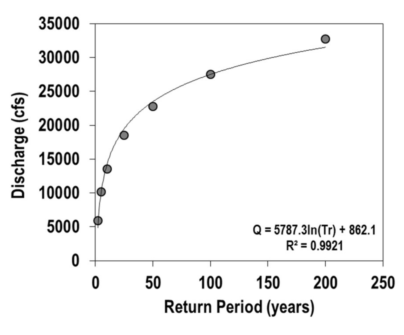
Log-Pearson Type III analysis of peak annual flows (1980–2016) was computed for the Le Sueur River gage near Rapidan, MN (USGS 5320500). This site was selected over gages used for the flow duration curve analysis because it has greater than 10 years of data and is downstream of all Maple and Le Sueur river camera sites. We used a standard flood frequency approach (e.g., the Oregon State University Streamflow Tutorial—Flood Frequency Analysis) to create Figure A5. Based on this analysis, the June 2014 and September 2016 floods were equivalent to 13- and 25-year recurrence interval floods, respectively. The magnitude of the 1.2-year event is 1.5 mm/day and or 1762 cfs.
Figure A6.
Number of days each year when mean daily flows are greater than the magnitude of the 1.5 mm/day or 1.2-year recurrence interval event. Daily data from USGS gage 5320500. Black line indicates an 11-year moving window average through the annual data points. Red bars indicate average annual values for the periods 1940–1979, 1980–2017, and 2014–2017.
References
- Wilkinson, B.H.; McElroy, B.J. The impact of humans on continental erosion and sedimentation. Bull. Geol. Soc. Am. 2007, 119, 140–156. [Google Scholar] [CrossRef]
- Montgomery, D.R. Is agriculture eroding civilization’s foundation? GSA Today 2007, 17, 4–9. [Google Scholar] [CrossRef]
- Hooke, R.L. On the history of human as geomorphic agent. Geology 2000, 28, 843–846. [Google Scholar] [CrossRef]
- Wilkinson, B.H. Humans as geologic agents: A deep-time perspective. Geology 2005, 33, 161–164. [Google Scholar] [CrossRef]
- Syvitski, J.P.M.; Vörösmarty, C.J.; Kettner, A.J.; Green, P. Impact of humans on the flux of terrestrial sediment to the global coastal ocean. Science 2005, 308, 376–380. [Google Scholar] [CrossRef] [PubMed]
- Owens, P.N.; Batalla, R.J.; Collins, A.J.; Gomez, B.; Hicks, D.M.; Horowitz, A.J.; Kondolf, G.M.; Marden, M.; Page, M.J.; Peacock, D.H.; et al. Fine-grained sediment in river systems: Environmental significance and management issues. River Res. Appl. 2005, 21, 693–717. [Google Scholar] [CrossRef]
- Belmont, P.; Gran, K.B.; Schottler, S.P.; Wilcock, P.R.; Day, S.S.; Jennings, C.; Lauer, J.W.; Viparelli, E.; Willenbring, J.K.; Engstrom, D.R.; et al. Large shift in source of fine sediment in the upper Mississippi River. Environ. Sci. Technol. 2011, 45, 8804–8810. [Google Scholar] [CrossRef] [PubMed]
- Dean, D.J.; Schmidt, J.C. The role of feedback mechanisms in historic channel changes of the lower Rio Grande in the Big Bend region. Geomorphology 2011, 126, 333–349. [Google Scholar] [CrossRef]
- Schottler, S.P.; Ulrich, J.; Belmont, P.; Moore, R.; Lauer, J.W.; Engstrom, D.R.; Almendinger, J.E. Twentieth century agricultural drainage creates more Erosive rivers. Hydrol. Process. 2014, 28, 1951–1961. [Google Scholar] [CrossRef]
- Lauer, J.W.; Echterling, C.; Lenhart, C.; Belmont, P.; Rausch, R. Air-photo based change in channel width in the Minnesota River basin: Modes of adjustment and implications for sediment budget. Geomorphology 2017, 297, 170–184. [Google Scholar] [CrossRef]
- Kelly, S.A.; Takbiri, Z.; Belmont, P.; Foufoula-Georgiou, E. Human amplified changes in precipitation-runoff patterns in large river basins of the Midwestern United States. Hydrol. Earth Syst. Sci. Discuss. 2017, 1–37. [Google Scholar] [CrossRef]
- Nakamura, F.; Seo, J., II; Akasaka, T.; Swanson, F.J. Large wood, sediment, and flow regimes: Their interactions and temporal changes caused by human impacts in Japan. Geomorphology 2017, 279, 176–187. [Google Scholar] [CrossRef]
- Call, B.C.; Belmont, P.; Schmidt, J.C.; Wilcock, P.R. Changes in floodplain inundation under nonstationary hydrology for an adjustable, alluvial river channel. Water Resour. Res. 2017, 53, 3811–3834. [Google Scholar] [CrossRef]
- Walling, D.E.; Owens, P.N.; Carter, J.; Leeks, G.J.L.; Lewis, S.; Meharg, A.A.; Wright, J. Storage of sediment-associated nutrients and contaminants in river channel and floodplain systems. Appl. Geochem. 2003, 18, 195–220. [Google Scholar] [CrossRef]
- Peck, M.; Gibson, R.W.; Kortenkamp, A.; Hill, E.M. Sediments Are Major Sinks of Steroidal Estrogens in Two United Kingdom Rivers. Environ. Toxicol. Chem. 2004, 23, 945. [Google Scholar] [CrossRef] [PubMed]
- Perks, M.T.; Owen, G.J.; Benskin, C.M.W.H.; Jonczyk, J.; Deasy, C.; Burke, S.; Reaney, S.M.; Haygarth, P.M. Dominant mechanisms for the delivery of fine sediment and phosphorus to fluvial networks draining grassland dominated headwater catchments. Sci. Total Environ. 2015, 523, 178–190. [Google Scholar] [CrossRef] [PubMed] [Green Version]
- Wood, P.; Armitage, P. Biological Effects of Fine Sediment in the Lotic Environment. Environ. Manag. 1997, 21, 203–217. [Google Scholar] [CrossRef]
- Bilotta, G.S.; Brazier, R.E. Understanding the influence of suspended solids on water quality and aquatic biota. Water Res. 2008, 42, 2849–2861. [Google Scholar] [CrossRef] [PubMed]
- Bennett, E.M.; Carpenter, S.R.; Caraco, N.F. Human Impact on Erodable Phosphorus and Eutrophication: A Global Perspective. Bioscience 2001, 51, 227. [Google Scholar] [CrossRef]
- United States Environmental Protection Agency (USEPA). National Water Quality Inventory: Report to Congress; EPA 841-R-16-011; USEPA: Washington, DC, USA, 2017.
- Belmont, P.; Foufoula-Georgiou, E. Solving water quality problems in agricultural landscapes: New approaches for these nonlinear, multiprocess, multiscale systems. Water Resour. Res. 2017, 53, 2585–2590. [Google Scholar] [CrossRef]
- Burt, T.P.; Allison, R.J. Sediment Cascades: An Integrated Approach. Sediment Cascades Integr. Approach 2009, 1–471. [Google Scholar] [CrossRef]
- Smith, S.M.C.; Belmont, P.; Wilcock, P.R. Closing the Gap Between Watershed Modeling, Sediment Budgeting, and Stream Restoration. In Stream Restoration in Dynamic Fluvial Systems: Scientific Approaches, Analyses, and Tools; Simon, A., Bennett, S., JM, C., Eds.; AGU: Washington, DC, USA, 2011; pp. 293–317. [Google Scholar]
- Kelley, D.W.; Brachfeld, S.A.; Nater, E.A.; Wright, H.E. Sources of sediment in Lake Pepin on the Upper Mississippi River in response to Holocene climatic changes. J. Paleolimnol. 2006, 35, 193–206. [Google Scholar] [CrossRef]
- Kelley, D.W.; Nater, E.A. Source apportionment of lake bed sediments to watersheds in an Upper Mississippi basin using a chemical mass balance method. Rivers 2000, 41, 277–292. [Google Scholar] [CrossRef]
- Wilcock, P. Identifying Sediment Sources in the Minnesota River Basin; Minnesota Pollution Control Agency: St. Paul, MN, USA, 2009. [Google Scholar]
- Gunderson, L.; Finley, R.; Bourne, H.; Lofton, D. Sediment Reduction Strategy for the Minnesota River Basin and South Metro Mississippi River: Establishing a Foundation for Local Watershed Planning to Reach Sediment TMDL Goals; Minnesota Pollution Control Agency: Saint Paul, MN, USA, 2014. [Google Scholar]
- Gran, K.; Belmont, P.; Bevis, M.; Cho, S.J.; Heitkamp, B.; Hobbs, B.; Marr, J.; Mielke, S.; Mitchell, N.; Kumarasamy, K.; et al. Collaborative for Sediment Source Reduction—Greater Blue Earth River Basin: Summary of Findings. Available online: http://www.bwsr.state.mn.us/drainage/dwg/resources/CSSR_Final_Report.pdf (accessed on 26 March 2018).
- Vaughan, A.A.; Belmont, P.; Hawkins, C.P.; Wilcock, P. Near-Channel Versus Watershed Controls on Sediment Rating Curves. J. Geophys. Res. Earth Surf. 2017, 122, 1901–1923. [Google Scholar] [CrossRef]
- Cho, S.J. Development of Data-Driven, Reduced-Complexity Watershed Simulation Models to Address Agricultural Non-Point Source Sediment Pollution in Southern Minnesota. Ph.D. Thesis, Johns Hopkins University, Baltimore, MD, USA, 2017. [Google Scholar]
- Ellison, C.A.; Savage, B.E.; Johnson, G.D. Suspended-sediment concentrations, loads, total suspended solids, turbidity, and particle-size fractions for selected rivers in Minnesota, 2007 through 2011. U.S. Geol. Surv. Sci. Investig. Rep. 2014, 5205, 43. [Google Scholar]
- Day, S.S.; Gran, K.B.; Belmont, P.; Wawrzyniec, T. Measuring bluff erosion part 2: Pairing aerial photographs and terrestrial laser scanning to create a watershed scale sediment budget. Earth Surf. Process. Landf. 2013, 38, 1068–1082. [Google Scholar] [CrossRef]
- Day, S.S.; Gran, K.B.; Belmont, P.; Wawrzyniec, T. Measuring bluff erosion part 1: Terrestrial laser scanning methods for change detection. Earth Surf. Process. Landf. 2013, 38, 1055–1067. [Google Scholar] [CrossRef]
- Wolman, M.G.; Miller, J.P. Magnitude and Frequency of Forces in Geomorphic Processes. J. Geol. 1960, 1, 54–74. [Google Scholar] [CrossRef]
- Runkel, A.C.; Meyer, G.N.; Lusardi, B.A. C-26 Geologic Atlas of Blue Earth County, Minnesota [Part A]; Minnesota Geological Survey: St Paul, MN, USA, 2011. [Google Scholar]
- Gran, K.B.; Belmont, P.; Day, S.S.; Finnegan, N.; Jennings, C.; Lauer, J.W.; Wilcock, P.R. Landscape evolution in south-central Minnesota and the role of geomorphic history on modern erosional processes. GSA Today 2011, 21, 7–9. [Google Scholar] [CrossRef]
- Gran, K.B.; Belmont, P.; Day, S.S.; Jennings, C.; Johnson, A.; Perg, L.; Wilcock, P.R. Geomorphic evolution of the Le Sueur River, Minnesota, USA, and implications for current sediment loading. In Management and Restoration of Fluvial Systems with Broad Historical Changes and Human Impacts: Geological Society of America Special Paper 451; James, L.A., Rathburn, S.L., Whittecar, G.R., Eds.; GeoScienceWorld: Mclea, VA, USA, 2009; pp. 119–130. ISBN 0072-1077r978-0-8137-2451-5. [Google Scholar]
- Schaffrath, K.R.; Belmont, P.; Wheaton, J.M. Landscape-scale geomorphic change detection: Quantifying spatially variable uncertainty and circumventing legacy data issues. Geomorphology 2015, 250, 334–348. [Google Scholar] [CrossRef]
- Smith, M.W.; Carrivick, J.L.; Quincey, D.J. Structure from motion photogrammetry in physical geography. Prog. Phys. Geogr. 2015, 40, 247–275. [Google Scholar] [CrossRef]
- Westoby, M.J.; Brasington, J.; Glasser, N.F.; Hambrey, M.J.; Reynolds, J.M. “Structure-from-Motion” photogrammetry: A low-cost, effective tool for geoscience applications. Geomorphology 2012, 179, 300–314. [Google Scholar] [CrossRef] [Green Version]
- Fonstad, M.A.; Dietrich, J.T.; Courville, B.C.; Jensen, J.L.; Carbonneau, P.E. Topographic structure from motion: A new development in photogrammetric measurement. Earth Surf. Process. Landf. 2013, 38, 421–430. [Google Scholar] [CrossRef]
- Carrivick, J.L.; Smith, M.W.; Quincey, D.J. Structure from Motion in the Geosciences; Wiley-Blackwell: Singapore, 2016; ISBN 978-1-118-89584-9. [Google Scholar]
- Girardeau-Montaut, D. Cloud Compare—3D point cloud and mesh processing software. Available online: http://www.danielgm.net/cc/ (accessed on 26 March 2018).
- Brasington, J.; Vericat, D.; Rychkov, I. Modeling river bed morphology, roughness, and surface sedimentology using high resolution terrestrial laser scanning. Water Resour. Res. 2012, 48. [Google Scholar] [CrossRef]
- Wheaton, J.M.; Brasington, J.; Darby, S.E.; Sear, D.A. Accounting for uncertainty in DEMs from repeat topographic surveys: Improved sediment budgets. Earth Surf. Process. Landf. 2010, 35, 136–156. [Google Scholar] [CrossRef]
- Castillo, C.; Pérez, R.; James, M.R.; Quinton, J.N.; Taguas, E.V.; Gómez, J.A. Comparing the Accuracy of Several Field Methods for Measuring Gully Erosion. Soil Sci. Soc. Am. J. 2012, 76, 1319. [Google Scholar] [CrossRef] [Green Version]
- Larsen, I.J.; Montgomery, D.R.; Korup, O. Landslide erosion controlled by hillslope material. Nat. Geosci. 2010, 3, 247–251. [Google Scholar] [CrossRef]
- Hovius, N.; Stark, C.P.; Allen, P.A. Sediment flux from a mountain belt derived by landsliding mapping. Geology 1997, 25, 231–234. [Google Scholar] [CrossRef]
- Lavé, J.; Burbank, D. Denudation processes and rates in the Transverse Ranges, southern California: Erosional response of a transitional landscape to external and anthropogenic forcing. J. Geophys. Res. Earth Surf. 2004, 109. [Google Scholar] [CrossRef]
- Stark, C.P.; Guzzetti, F. Landslide rupture and the probability distribution of mobilized debris volumes. J. Geophys. Res. Earth Surf. 2009, 114, 1–16. [Google Scholar] [CrossRef]
- Doyle, M.W.; Shields, D.; Boyd, K.F.; Skidmore, P.B.; Dominick, D. Channel-Forming Discharge Selection in River Restoration Design. J. Hydraul. Eng. 2007, 133, 831–837. [Google Scholar] [CrossRef]
- Minnesota Department of Natural Resources September 20–22, 2016 Heavy Rain. Available online: http://www.dnr.state.mn.us/climate/journal/160921_22_heavy_rain.html (accessed on 10 January 2018).
Figure 1.
Locations of bluff study sites within the Greater Blue Earth River basin. Inset photo corresponds with bluff site LS10, a 20-m-tall bluff composed of overly consolidated glacial till; 1.8-m-tall person for scale. Streamflow gages are labeled by number (1: Le Sueur River gage near Rapidan, MN (USGS 5320500), 2: Le Sueur River near Highway 8 (MPCA/MDNR site 32076001), 3: Maple River at Highway 35 (MPCA/MDNR site 32072001), 4: Big Cobb River near Beauford (MPCA/MDNR site 32071001), 5: Blue Earth River near Rapidan (USGS 05320000), 6: Watonwan River near Garden City (MPCA/MDNR site 31051001)). Photo taken following a large flood event in June 2014 (credit: Shayler Levine).
Figure 2.
(a) Average number of failure days per month for a bluff of average size 250 m2 (along stream length × height). Number of observations: 2705; (b) Average number days with large failures per month. Number of observations: 347. Months are labeled in order from January (1) to December (12).
Figure 2.
(a) Average number of failure days per month for a bluff of average size 250 m2 (along stream length × height). Number of observations: 2705; (b) Average number days with large failures per month. Number of observations: 347. Months are labeled in order from January (1) to December (12).

Figure 3.
Panels of change from seven repeat structure-from-motion survey-generated DEMs of difference (below) and distributions of volumetric change (m3) as a function of depth of change (m) (above) for site LS9 (a) and LS10 (b); outputs from ArcMap 10.4, Geomorphic Change Detection software 5.0. All survey areas are plotted relative to the same black bar indicating approximately the maximum length of each bluff surveyed. Bluff geomorphic change surveys shown perpendicular to the streamwise direction; flow direction from left to right for site LS9, and right to left for site LS10.
Figure 4.
(a) Bluff retreat scaling relation (black line) between net bluff erosion volume (V) and bluff survey area (A) from repeat SfM surveys and Day et al. 2013a TLS surveys, 111 total observations. (b) Local scaling relation between measured total bluff erosion volume (V) and bluff erosion survey area (A) from repeat SfM surveys, 42 total observations. Data represented by green triangles were estimated using the locally measured erosion relation.

Figure 5.
Distributions of large toe and face failures plotted as kernel density functions of flow exceedance probabilities. Dashed vertical line indicates 15% exceedance probability flows. Behind the kernel density functions, four flow duration curves are plotted, corresponding to gages for each of the bluff sites (described in Section 2.3.4); BE: Blue Earth River sites, LS: Le Sueur River sties, MPL: Maple River sties.
Figure 6.
(a) Large face failure frequency (total number of days per month), average daily retreat rate for a 250 ± 95 m2 bluff in a given month, and their product, total bluff retreat, measured across 20 time lapse photo monitored sites, 169 total observations. (b) Same data as 6a, only plotted against daily flow exceedance probability. Data binned every 10 percentiles except percentiles binned 0–2 and 2–10. Data binned as 0–0.02 exceedance probability only include June 2014 and September 2016 flood peaks, when 12% of all large failures occurred. Total bluff face erosion during the two flood peaks account for 45% of all face erosion from June 2014–May 2017. Data represented by one hundred fifty seven total observations since 12 large face failures occurred when daily flow data were unavailable due to winter ice affected gages.
Figure 7.
(a) Spatially averaged event retreat rate (m/day) from time lapse photo estimated erosion versus the failure date flow exceedance probability. Points are color-coded by the persistence time of the failed till material; (b) box-and-whisker (25% and 75%) plots of flow exceedance probabilities associated with categorical failed till persistence times. Black bar and grey circle indicate median and mean descriptive statistics, respectively, and n indicates the number of observations in each category; (c) till event retreat rate versus daily discharge normalized by drainage area upstream of gauge. Line indicates a weak power law relation between event size and discharge; (d) same as (c), but regression applied only to events when daily discharge was greater than 1 mm/day; (e) same as (c), but regression applied only to events that persisted for less than one week.
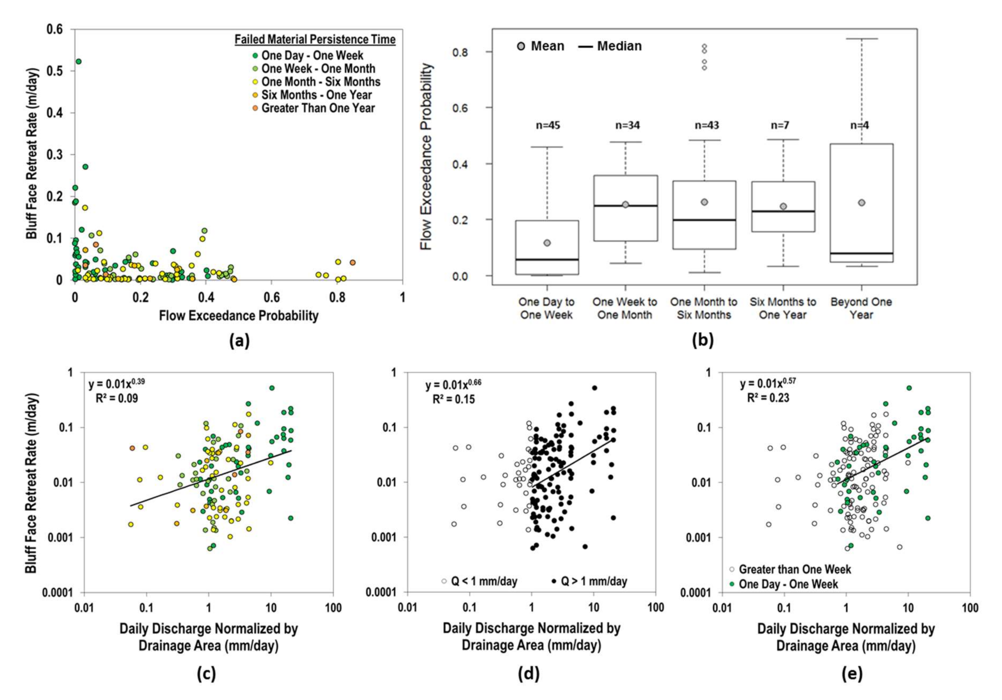
Figure 8.
Streamflow frequency, days greater than 1.5 mm/day runoff (orange); bluff erosion magnitude, given the bluff erosion (E)-discharge (Q) power law relation (green line fitted through green points); and the product of bluff erosion magnitude and streamflow frequency versus river basin runoff (mm/day), during the periods (a) 2014–2017 and (b) 1940–2017. Mean daily runoff values for the Le Sueur River gage near Rapidan, MN (USGS 5320500).
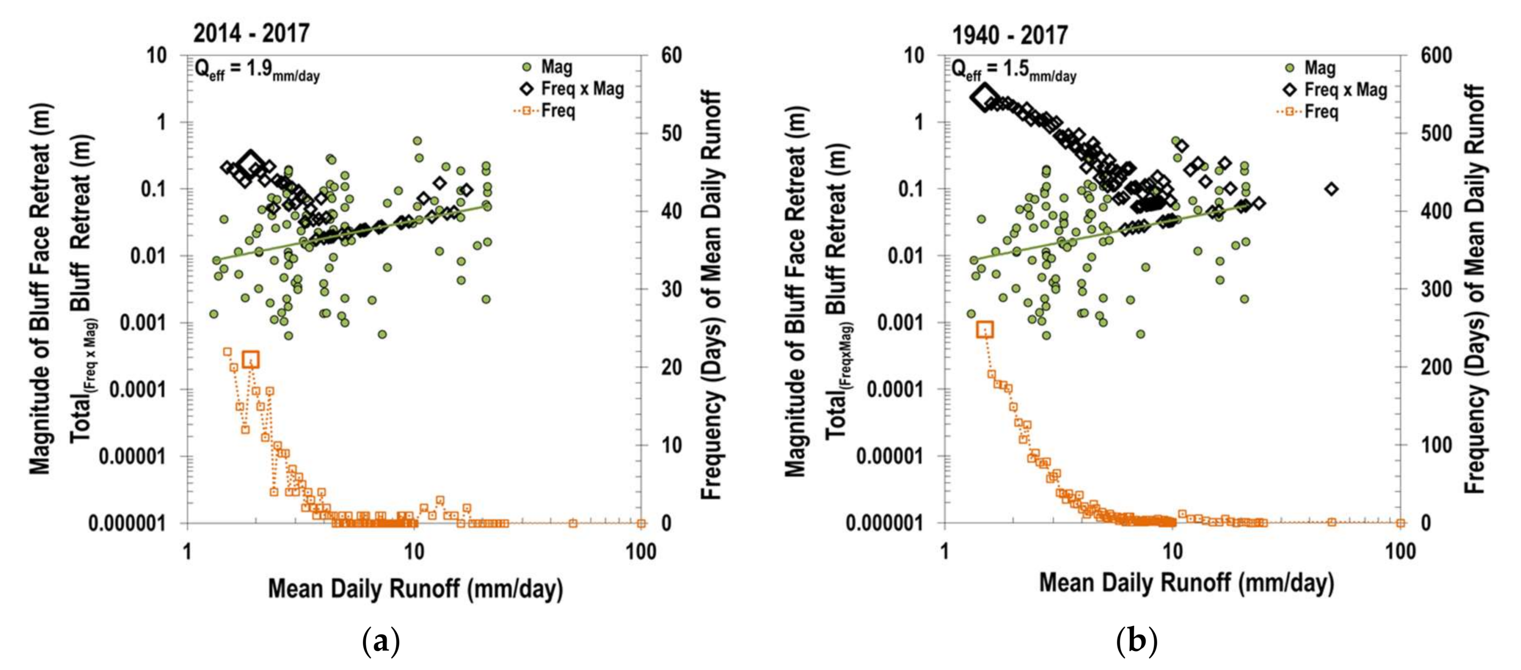
Table 1.
Repeat Structure-from-Motion photo survey information. Abbreviations used for ground control points (GCPs) and root-mean-square error (RMSE).
Table 1.
Repeat Structure-from-Motion photo survey information. Abbreviations used for ground control points (GCPs) and root-mean-square error (RMSE).
| Site Name | Survey Date | Number of Survey Photos | Number of GCPs | GCP RMSE (m) | Total Dense Cloud Points (×106) | Average Cloud Density (pts/cm2) |
|---|---|---|---|---|---|---|
| LS9 1 | 6/15/2014 | 46 | 9 | 0.024 | 28.4 | 1.4 |
| LS9 | 7/3/2014 | 52 | 11 | 0.087 | 35.1 | 1.5 |
| LS9 | 5/8/2015 | 55 | 9 | 0.013 | 30.3 | 1.3 |
| LS9 | 7/12/2015 | 60 | 11 | 0.028 | 17.9 | 0.6 |
| LS9 | 5/24/2016 | 54 | 10 | 0.031 | 17.7 | 0.7 |
| LS9 | 10/22/2016 | 100 | 11 | 0.024 | 22.0 | 0.8 |
| LS9 | 5/17/2017 | 108 | 10 | 0.010 | 47.1 | 1.6 |
| LS10 2 | 6/15/2014 | 51 | 9 | 0.015 | 31.9 | 2.2 |
| LS10 | 7/3/2014 | 110 | 13 | 0.018 | 35.1 | 1.7 |
| LS10 | 5/9/2015 | 51 | 11 | 0.010 | 38.6 | 2.0 |
| LS10 | 7/10/2015 | 50 | 11 | 0.073 | 19.9 | 0.7 |
| LS10 | 5/24/2016 | 63 | 10 | 0.018 | 26.1 | 1.0 |
| LS10 | 10/22/2016 | 100 | 13 | 0.018 | 20.6 | 0.7 |
| LS10 | 5/17/2017 | 91 | 5 3 | 0.016 | 38.7 | 1.3 |
1 Bluff LS 9 average survey area: 2100 m2. 2 Bluff LS 10 average survey area: 2000 m2. 3 Field survey contained 12 Ground Control Points (GCPs), but only 5 GCPs were recovered post-survey due to instrument damage.
© 2018 by the authors. Licensee MDPI, Basel, Switzerland. This article is an open access article distributed under the terms and conditions of the Creative Commons Attribution (CC BY) license (http://creativecommons.org/licenses/by/4.0/).
Share and Cite
MDPI and ACS Style
Kelly, S.A.; Belmont, P. High Resolution Monitoring of River Bluff Erosion Reveals Failure Mechanisms and Geomorphically Effective Flows. Water 2018, 10, 394. https://doi.org/10.3390/w10040394
AMA Style
Kelly SA, Belmont P. High Resolution Monitoring of River Bluff Erosion Reveals Failure Mechanisms and Geomorphically Effective Flows. Water. 2018; 10(4):394. https://doi.org/10.3390/w10040394
Chicago/Turabian StyleKelly, Sara Ann, and Patrick Belmont. 2018. "High Resolution Monitoring of River Bluff Erosion Reveals Failure Mechanisms and Geomorphically Effective Flows" Water 10, no. 4: 394. https://doi.org/10.3390/w10040394
Note that from the first issue of 2016, this journal uses article numbers instead of page numbers. See further details here.