An Analysis of the Potential Impact of Climate Change on the Structural Reliability of Drinking Water Pipes in Cold Climate Regions


Norwegian University of Science and Technology, Trondheim 7491, Norway
*
Author to whom correspondence should be addressed.
Water 2018, 10(4), 411; https://doi.org/10.3390/w10040411
Submission received: 22 February 2018
/
Revised: 28 March 2018
/
Accepted: 29 March 2018
/
Published: 1 April 2018
Abstract
:The climate is changing worldwide. For the northern hemisphere there are distinct challenges related to climate change. It is expected that temperature on a general basis will increase within the next 100 years, and that the increase will be most severe during winter months. The literature shows a correlation between temperature and failures. This correlation is most evident for smaller grey cast iron pipes, and for pipes which is constructed in trenches vulnerable to frost heave. A comprehensive amount of failure data (over 25,000 failures) has been gathered from Norwegian cities in order to quantify the correlation between temperatures and failure rates. The analysis supports the findings in the literature, by establishing a statistical significant correlation, which states that failure rates increase with falling temperatures. At the same time, the expected increase in future temperatures has been used to analyze the impact on failure rates within 2070. The results show that the increasing temperatures will have a positive effect on failure rates. It can be expected that failure rates will be reduced by 2.7% to 7.2% within 2070, depending on the climate scenario.
1. Introduction
The world’s climate is changing. There are distinct changes happening in the globes’ northern hemisphere, which is understood as a cold climate region. These are inherently different from climate change in warmer climates. It is expected that cold climate regions will experience warmer temperatures, a changing temperature pattern with more extreme cold events, more precipitation and more intense rainfall events due to climate change [1]. The highest temperature increase is expected during the winter months [2], which can result in less ice and snow covers during the winter [1] and less problems with frost heave of the ground. However, extreme cold weather events have been widely reported through media outlets during recent years in several cold climate regions, with the side effect of increased water main breaks [3,4,5]. It might be that such circumstances are an additional effect of the changing climate. Sometimes these events are caused by increased movement of the northern polar vortex, where Arctic air escapes and spills southward bringing Arctic weather with it. This has lately been observed over Northern America [6,7] and Europe [8].
Climate change will also lead to droughts occurring more often and over longer periods of time [1]. Droughts are more likely to occur in warm climate regions, such as the southern part of Europe, rather than in cold climate regions. However, the city of Bergen in Norway, which has an annual average precipitation of 2250 mm, experienced a drought both in the winter of 2006 [9] and 2010 [10], leading to a threat against the ability to supply drinking water. The reason for these kinds of droughts is a change in the precipitation patterns, with extremes of both rainfall intensity and droughts being intensified.
The average annual air temperatures are increasing worldwide [11,12] and in cold climate regions like Norway [13]. In Norway, even the winters have generally been warmer for the past 30 years than the 45 years before that (except for the warm winters of 1970–1975) [14]. The period from 1983 to 2013 is likely the warmest 30-year period in the northern hemisphere for the last 800 years.
There are verifications in the literature that water pipe failures are dependent on temperature and that an increased number of failures correlate with colder winter months [15,16,17]. The case studies presented in this literature looked at correlation between number of failures and month, and between failure rates and season. Any correlation between specific temperatures and failure rates has therefore not been produced. Makar [18] lists frost loading as an important factor for failures in northern climates. A Norwegian case study for the city of Oslo has shown the same kind of correlation [19]. Another case study from the city of Lyon, France [20], shows that 51% of the number of failures happen during the months of December, January and February, and found a statistical trend between the weather variable of ‘negative air temperatures’ and failures for the month of December, with a confidence interval of 98%. The analysis was based on a time series of 18 years of pipe failure data.
Colder temperatures lead to frost heave of the ground and can cause severe mechanical strain on the pipes and the pipe connections [21,22,23], and are thus expected to have some form of impact on the failure rates. Both cold temperatures with its frost heave effect and the frosting and thawing cycles can cause trouble for the pipes during the colder winter months, causing soil movement, alternating movement and freezing of the surrounding soil, and pipe-soil interactions. Makar (1999) [18] further states that changes of the soil temperature lead to thermal stresses in the ground, which can cause pipe failures.
The case study of Oslo [19] shows that 52.5% of registered failures are transverse fractures. We have looked into the failure data of the 9 largest water utilities in Norway to find that failure data shows that 51% of the failures are transverse fractures. This fracture mode therefore dominates the failure data of many big Norwegian cities. Transverse fractures, sometimes referred to as circumferential cracks, is normally caused by bending forces on the pipes [24], which can be produced by settling of the soil and frost heave. According to Makar (2001) [24], transverse fractures are the most common failure mode on small grey cast iron pipes, while longitudinal fractures are more common to large diameter pipes. Since most networks have an abundance of smaller diameter pipes, this might explain some of the predominance of transverse fractures in the Norwegian failure data, and in the case study by Rajani et al. [17]. Rajani et al. [17] looked into the mode of water mains failures, and found that about 70% were circumferential, e.g., transverse fractures. These breaks primarily occurred during the winter, and they suggest a pipe-soil interaction to be the underlying cause, thereby blaming frost heavy processes. The case study of Reikvam [19] shows a doubling of transverse failures during the winter months, thus verifying the assumption of Rajani et al. [17]. Other types of failure modes in the case study of Reikvam [19] do not show the skewed distribution of failures between winter and summer months, but rather a predominance of failures in the summer months. The study by Reikvam [19] found that grey cast iron is the material that is predominantly affected by increased failure rates during winter months. The findings show a 60% distribution of failures on grey cast iron pipes during winter. For other materials the distribution is not as evident. In addition to grey cast iron pipes being the main cause for increased failures during winter, the construction period of post World War 2 (1945–1965) shows the same trend, with 65% of the number of failures recorded during the winter. This period is known in Norway for its poor quality of trench work, and we believe that this has caused the trenches and the pipes to be more exposed to frost heave. When the trench is more exposed to frost heave, it will naturally be more exposed and vulnerable for tension loading and pipe bending which, as discussed above, is one of the main reasons for transverse fractures. The case studies and literature therefore show us why pipes, and evidently some pipe materials more than others, are more vulnerable to increased failure rates during the winter. The literature supports one of the main hypotheses of the paper, which is that failure rates are affected negatively by decreasing temperatures, and that failure rates therefore will be higher in the winter than in the summer months.
If we can show that there is a correlation between pipe failures and temperature, we can derive that the future expected temperature increase is positive news for the drinking water networks with regard to failure rates. This paper tries to approach the subject matter with a clearly defined hypothesis, which is to be tested on the large-scale Norwegian data set of failures on drinking water pipes, with associated climate data. The hypothesis to be tested is the following:
- ○
- Hypothesis: Pipe failures and failure rates are correlated to frost heave of the ground, and thereby also correlated to air temperature.
The objectives of the paper can be seen in light of the hypothesis. The first objective is therefore to prove or disapprove the hypothesis. If the hypothesis turns out to be non-falsifiable with the data we have available, a second objective is to establish a linear regression model which correlates failure rates to temperature and thus gives a quantifiable impact of temperature on failures. A third objective is to relate future climate models on expected temperature increase to the linear regression model, in order to quantify the impact of climate change on future failure rates. The projection period is 50 years into the future. This will make it possible to discuss if the reliability of drinking water networks in cold climates will be affected by climate change in the long-term.
The paper’s first objective does not contribute anything to current state of the art, since literature already shows that there are correlations between failures and temperature. There is however a research gap between this knowledge and knowing how a changed future climate (and thus changed temperatures) will impact failure rates. If the second objective can be fulfilled it will contribute to current state of the art with an equation that states the quantifiable relationship between failure rates and temperature. If the third objective can be fulfilled it will further contribute with data about expected future changes in failure rates based on climate change, which can be used by water managers in the long-term management of urban drinking water networks.
Reliability of Pipes
Reliability is by ISO 8402 defined as the ability of an element or an asset to perform a necessary function under given operational and environmental conditions, for a given time period. There are different ways to consider the reliability of an asset or an urban water network, albeit hydraulic and structural reliability are the two most common approaches. The structural reliability, which is the one considered in this paper, is about considering the structural integrity of the physical network. Pipe failures is the parameter that we will use in this paper to represent the structural reliability of the water network. From a structural point of view, the reliability of the water network is under attack in the winter months, both in cold climate regions [17,19] and in the more tempered regions of Central Europe [15,16,20]. The potential impact of climate change on structural reliability will be examined in this paper through the analysis of the correlation of failure rates and air temperature, while addressing the expected future change in air temperature.
2. Method
The method is based on testing the hypothesis generated in Section 1 and, if found to be statistically viable, estimate the future impact of climate change on failure rates. The hypothesis was therefore tested by doing the following data analysis:
- •
- Failure rates (number of failures per temperature per day) will be plotted against same day temperature and against the average temperature of the preceding week. Plotting failure rates instead of number of failures will adjust the data correctly since there are more days registered with warm temperatures than with cold temperatures. The potential correlation will be tested with a linear regression model, and the model will be statistically tested for a certain confidence level.
The procedure is based on an analysis of extensive amounts of data. 25,573 registered failures on drinking water pipes were collected from nine of the largest cities in Norway, spanning observation windows of failures that varied between 20 and 39 years (it varied between utilities). The amount of data is so extensive that the authors wanted to assess any correlation between climate data and the failures, and if statistically viable, quantify the correlation. Two approaches to analyze this potential correlation were adapted:
- Failures were analyzed directly against the temperature on the day the failure occurred.
- Failures were analyzed against the average temperature one week preceding (including the day of the failure) the relevant failure.
These two approaches relate to step 2.1 and 2.2 in Figure 1. A statistically proven correlation up to a certain confidence level would lead into step 2.3, which included analysis of future climate scenarios with regard to temperature increase. In step 2.4, the linear regression found in 2.2 would be analyzed against expected temperatures across the seasons in 2070 in order to quantify an expected decrease or increase in future failure rates.
2.1. Preparing and Plotting Failure Data
The procedure of the analysis was performed in the following steps:
- (a)
- Gathering of failure data. Identification of reliable failure data for each city, which is the relevant observation window. This is based on an assessment of when the utility started to collect failure data in a structured way.
- (b)
- Historical temperature data for the relevant cities was collected from a national database (at www.senorge.no).
- (c)
- Failures were correlated to temperature through dates given for the failure events.
- (d)
- Number of failures per temperature were counted = F/temp.
- (e)
- Number of days per temperature were counted = D/temp.
- (f)
- Historical failure rates (failures per day) per temperature were calculated by Equation (1).
- (g)
- Failure rates (step f) were plotted against temperature.
Fr = Historical failure rate for a given temperature.
F/temp = number of failures per temperature (from step d).
D/temp = number of days per temperature (from step e).
2.2. Analyzing Correlation between Failure Rates and Temperature
We saw that for the most extreme temperatures, both warm and cold, the failure rates deviated from the correlation found in the other data. Due to the few number of days registered with these cold and warm temperatures, we identified the few observed days to be an issue. In order to avoid distorting of the correlation by data with limited registrations, we decided to base the correlation exclusively on temperatures that were registered with number of days within one standard deviation of the average of the number of days registered per temperature. This meant that temperatures with number of days outside of (less than) one standard deviation of the average were omitted from the analysis. In order to plot the correlation we therefore did the following:
- (h)
- Calculation of average number of days registered per temperature according to Equation (2).
- (i)
- Calculation of standard deviation for the number of days registered per temperature.
- (j)
- Calculation of the minimum number of days needed for being part of the correlation calculation, based on the numbers found in points h and i.
- ○
- More specifically: minimum number of days registered for a single temperature = average number of days registered per temperature (1834 days)—standard deviation (1762 days) = 72 days.
- ○
- In order to include a temperature in the correlation analysis, we needed 72 days or more registered of the temperature.
- (k)
- Plotting failure rates (failures/temperature/day) versus temperature.
- (l)
- Calculating linear regression with R and R2 values.
- (m)
- Statistically quantify the uncertainty of the regression line by performing a test of hypothesis of the linear correlation.
- (n)
- If statistically viable, establish the regression line as a model on the impact of temperature on failure rates, with a given uncertainty.
- (o)
- We assume that failures occurring during the summer, i.e., during warm temperatures, are not dependent on temperature. The failures occurring during these temperatures are therefore exclusively dependent on other parameters, like deterioration, hydraulic pressure, corrosion etc. The failure rate during these temperatures therefore constitutes the ‘baseline’ failure rate of the pipes. This approach is also considered in Le Gauffre et al. [20]. The failure rate for the warmest temperature was at 0.21 failures/temperature/day (based on the linear regression), constituting the baseline failure rate.
D average = Average number of days registered per temperature.
n = 25 is maximum positive temperature in the temperature range. The total number of temperatures in the analyzed temperature range is 49, ranging from −23 to 25 degrees Celsius.
i = first temperature in range, in this case the coldest temperature at—23 degrees Celsius.
The same line of procedure was used to determine if there is any correlation between failure rates and the average temperature of the preceding week, as given by approach number 2.
2.3. Preparing Data for Expected Future Temperature Increase
When the correlation was given and its regression line tested for uncertainty, the current impact of temperature on failures was established. In order to see how the impact of temperature changes in the future might impact failures, we used results from a Norwegian Environment Agency (Governmental department) report on the climate in Norway within the year 2100 [2]. The report presents results on future expected temperature increases based on different climate change models, termed as Representative Concentration Pathways (RCP), which describe different scenarios with regards to future development of global greenhouse gas emissions. The modelling is based on three RCP scenarios and three levels of uncertainty, so-called 10-percentile (low), median (medium), and 90-percentile (high) values. The data were scaled down to Norwegian conditions based on two different downscaling processes. The procedure to assess expected temperature increase in 2070 was performed in the following steps:
- (p)
- From the Norwegian Environment Agency report, we gathered reliable data on the potential future temperature increase. The estimated future temperature increase was based on the following reasoning:
- ○
- Values from three scenarios for future greenhouse gas emissions were used. They represent different expected temperature increases.
- ○
- Only median values of the climate scenario predictions were used, as they refer to the value in which 50% of the projection values are larger and 50% of the projection values are smaller. The median therefore represents a most probable outcome, as it represents a middle way between more extremes.
- ○
- T downscaling processes were used in the National Agency report. One downscaling process modelled three of the RCP scenarios, while the other downscaling process modelled two of the scenarios. Where the two downscaling processes modelled the same RCP scenario, an average of the expected temperature value was used.
- ○
- The estimated temperature increase varies by the season, so an expected temperature increase was calculated per season for the three RCP scenarios.
- ○
- The three RCP scenarios represent the following [2]:
- ◾
- RCP 2.6: Emissions are reduced drastically after 2020, and will be close to 0 within 2080.
- ◾
- RCP 4.5: Emissions are reduced after 2040, and in 2080 emissions are on a level that correspond to 40% of emissions in 2012.
- ◾
- RCP 8.5: ‘Business as usual’ scenario, where the increase in emissions follow the same pattern as today.
- ◾
- The values given after RCP relates to the estimated extra heat supply, given in W/m2, for the emission scenario.
- ○
- A linear increase in temperature from the reference period (1971–2000) to the projection period (2071–2100) was assumed. This was done since no time series of the future temperature increase is available for the Norwegian-based temperature data (only the estimate for the projection period). Even though historic Norwegian temperature data fluctuates, it is possible to create a linear approximation to the data series for the past 50 years or so [2], supporting our claim that it can also be done for future temperature increase.
- ○
- The modelling in Hanssen-Bauer et al. [2] is based on a temperature increase from the reference period of climate in Norway, which is from 1971 to 2000. The increased temperature is projected towards the period of 2071 to 2100. From the middle of the reference period to the middle of the projection period there is 100 years (1985 to 2085). The objective of this paper is to predict the impact of climate 50 years into the future. Our year of focus is therefore roughly 2070. In 2070 we assumed that about 85% of the expected temperature increase has occurred. We based this assumption on the following principles:
- ◾
- We assumed that the temperature increase from today to the projection period is linear, as argued in the previous point.
- ◾
- 2070 is 85% towards 2085 (when the linear increase is assumed).
- ○
- According to Hanssen-Bauer et al. [2], the expected temperature increase during spring looks like the expected increase during fall, with small deviations. For this paper, we therefore looked at spring and fall as a common group representing a single season. We looked at temperature increases during three seasons; summer, winter and spring + fall.
- (q)
- In order to relate temperature to season, we assumed a temperature range for each season. We divided the temperature data into three intervals to represent the three seasons:
- ○
- Summer: warmer than 12 degree Celsius.
- ○
- Winter: colder than 0 degree Celsius.
- ○
- Spring + fall: between 0 and 12 degree Celsius.
This gave us the necessary data to predict the future impact of temperature on failures, and consequently, on the drinking water network reliability. Figure 2 presents an illustration of the data we used to predict this impact. The figure shows how the impact of temperature on failures increases with negative values of temperature, and how the temperature curve is ‘moved’ to the right due to the future expected temperature increase. The figure also shows the number of days and the number of failures registered per temperature. This data shows us why the failure rates are higher in the winter months, as we can see that the columns for number of failures are as high, or higher, than the graph for number of days when the temperature is low. We can see that the distance between these two starts to increase just as soon as the temperature reaches zero degrees, and warmer. This equates to higher failure rates during colder months.
2.4. Analyzing the Future Impact of Climate on Failures
In order to calculate the future impact of warmer temperatures on failure rates, we performed the following steps. All steps were performed for each of the three climate change scenarios.
- (r)
- The temperature range was divided into the three seasons as stated in segment q. The temperature range was from −23 to 25 degrees Celsius, and is illustrated in Figure 2. We now also looked at temperatures outside of the standard deviation calculated in segment j. An expected average future temperature increase was established based on the process described in segment p. These temperatures are given in Table 1.
- (s)
- Expected temperatures for 2070 were calculated by increasing the historical summer, winter and spring + fall seasons with the temperatures given in Table 1.
- (t)
- Calculation of the historical failure rate for each temperature by Equation (1), same as step f.
- (u)
- Calculation of the share of the failure rates that are caused or driven by temperature, as given by Equation (3). The baseline failure rate was set to 0.21 failures/temperature/day (from segment o).
- ○
- The total failure rate at each temperature was given by the linear regression equation (Equation (9)).
- ○
- The share of the failure rate which is driven by temperature increases with negative temperatures in a linear fashion, in the exact same rate as the linear regression line. This is illustrated in Figure 2.
- (v)
- For the historic data, an expected number of failures (for each temperature) driven by temperature was calculated according to Equation (4). This gave us a historic number for failures, which were probably temperature driven.
- (w)
- For 2070 we calculated an expected number of failures caused by temperature (for the range of temperatures from −23 to25 degrees Celsius) with Equation (5).
- ○
- For this we took into consideration the ‘movement’ of the temperature curve to the right, as illustrated in Figure 2. The curve is ‘moved’ by the temperature increase calculated in segment s.
- (x)
- An increase or reduction in expected number of failures in 2070 was calculated for each temperature (from −23 to 25 degrees Celsius) with Equation (6). This gave us a comparison between historical failures driven by temperature and expected number of failures in 2070 driven by temperature.
- (y)
- By accumulating the numbers found for each temperature in segment x, we could calculate the total number of increased or reduced failures across the entire temperature range, in total in 2070, compared to the historical data. This was done with Equation (7).
- (z)
- The accumulated number in segment y was then used to calculate the % of increase or decrease of expected failures within 2070. Equation (8) was used for this. This calculation was done for each of the three climate scenarios. The results can be used to discuss the impact of climate on the reliability of the drinking water network through the impact on failures and failure rates.
Fr% = share of failure rate (given in %) caused by temperature for a given temperature.
(−0.0047x + 0.321) = Linear regression model (Equation (9)).
x = given temperature, ranging from −23 to 25 degrees Celsius.
where
Number of failures share = number of historical failures caused by temperature for a given temperature.
where
Number of failures share 2070 = number of expected failures in 2070 caused by temperature for a given temperature.
Displaced D/temp = number of historical days registered for a temperature which is X degrees colder than the relevant temperature. The X degrees ‘displacement’ is governed by climate scenario and by season, and is defined in Table 1. This is based on the assumption that the shape of the distribution of days across temperatures will be the same in 2070 as in the past, but that the distribution will be displaced towards warmer temperatures. See Figure 2 for illustration of this concept. The size of the temperature displacement is governed by climate scenario (given in Table 1).
where
Fchange per temp = Change in expected number of failures per temperature in 2070.
where
Fchange total = Change in total expected number of failures in 2070. The number of failures are accumulated across the temperature range.
n = 25, maximum temperature.
where
% Fchange total = the percent of total increase or decrease of expected failures (across the temperature range) within 2070 compared to historical number of failures.
25 573 = total historical number of failures registered across the temperature range.
3. Results
3.1. Pipe Data
The networks of the nine cities that were investigated consist of mostly grey cast iron, ductile iron and PVC pipes. Grey cast iron and ductile iron constitute between 60% and 80% of the networks in seven of the cities. Two of the cities have a degree of PVC which amounts to about 50% of their networks length. A variation of other materials, like PE, asbestos cement and steel, constitute the remaining part. The total length of the networks varies between 296 and 1421 km, while average age varies between 32 and 60 years. All of the cities have pipes that are from the 1800’s. The oldest pipe in operation is from 1859. All types of diameters occur in the networks, ranging from very small diameters of 20 mm up until very large diameters of 1200 and 1600 mm. The main bulk of diameters are however found in the less than 200 mm range.
The failures analyzed in the paper include failures that have occurred on pipes that now are either decommissioned or have been renovated with no-dig. This means that some of the failures are connected to pipes that are no longer in operation.
3.2. The Baseline Failure Rate
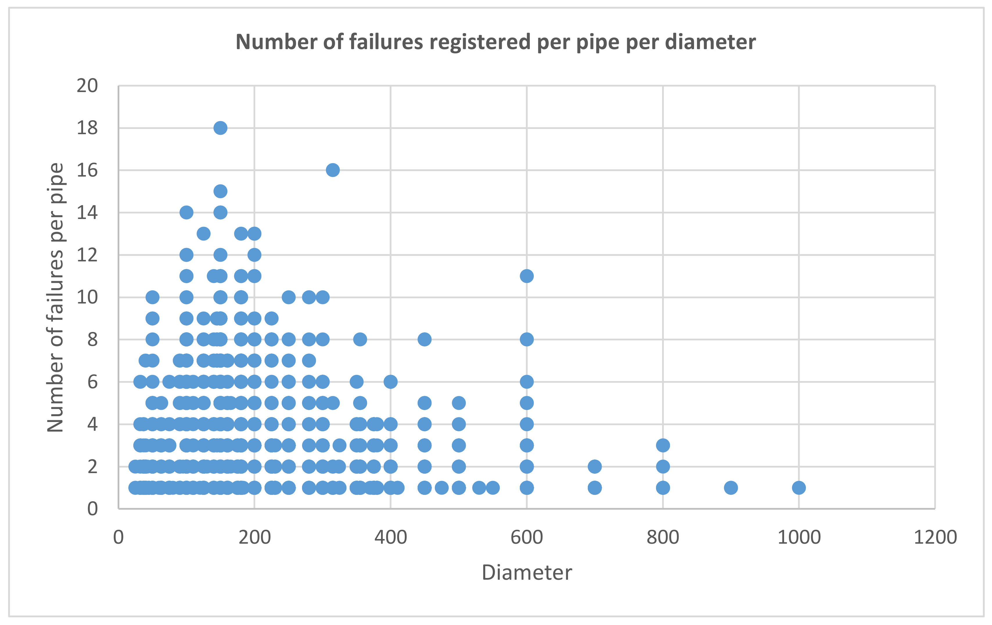
Before going into the results of the correlation analysis, we present two figures relating to the influence of pipe features on failures. This give us some understanding of the baseline failure rate that is described in segment o in the method chapter. The baseline failure rate is calculated (based on the linear correlation) to be 0.21 failures/temperature/day. The failures contributing to this rate is caused, among other things, by deterioration, high hydraulic pressure, different types of corrosion, mechanical stress, type of soil, heavy traffic loads etc. These factors will in varying degree contribute to baseline failure rates, and will be dependent on local situations, local geology, pipe materials, history of the network and management principles. Figure 3 and Figure 4 give us some understanding of some of these factors. Figure 3 presents number of failures related to diameter, and it shows a correlation between decreasing diameters and number of failures, both in total amount and in recurring failures in a pipe. The total amount of failures is higher when the density of the failures (the blue dots) are higher, and recurring failures are higher when the number of failures per pipe (y-axis) is higher. The worst performing diameters are between 100 and 200 mm. In this area there are also many pipes with a high number of recurring failures. It is also natural that these pipes have a higher number of failures since there are a lot more of these pipes than pipes with large diameters in the network. Failures related to small diameters can be explained by all of the mentioned factors, but are usually more vulnerable to corrosion than larger pipes due to their thinner pipe wall thickness.
Figure 4 presents number of failures related to construction year. The history of the construction of water pipes in Norway is fairly well known, and the weakness of certain periods show itself through failure data. The post World War 2 period, ranging from 1945 to the mid 1960s is known for the first use of machines to dig the trenches. Along with the introduction of machine digging followed poor trench work. Everything was done fast and with little focus on quality of the work or quality of the filling material. This has led to extensive problems with pipes in this period, caused by mechanical stress movement of the ground, frost heave and general deterioration. At the same time, lack of corrosion protection in ductile iron pipes and poor production standard of plastic pipes laid before the 1980s have led to unusual high numbers of recurring failures in these type of pipes. These are some of the main reasons for the increased recurrence of failures from 1940 to 1980 in Figure 4. In some Norwegian cities there is also a lot of marine clay. These cities experience extensive problems with ductile iron pipes combined with marine clay as the surrounding type of soil. Concerning soil types and their influence on failures, marine clay has been singled out as a major contributor to increased failure rates in certain Norwegian cities.
3.3. Correlation of Pipe Temperature
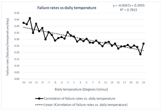
Figure 5 presents a plot of failure rates (failures/temperature/day) versus temperature. A linear correlation is plotted based on the data, with an accompanying equation and an R2 value. The linear regression shows a trend of an inverse correlation between increasing failure rates and temperatures. The R2 value shows that 78.2% of the total variation in the data can be explained by the linear regression model.
3.3.1. Linear Regression Model
The regression line adapted in Excel with the least squares method has the following equation:
The slope is −0.0047 and the point of intersection is 0.321. The negative slope shows that there is a negative linear correlation between the failure rates and temperature. The correlation coefficient R and the coefficient of determination R2 for the regression line is −0.884 and 0.782, respectively. An R2 value of 0.782 means that 78.2% of the variations in y can be explained with x, while 21.8% of the variations are caused by other factors. Since we only have estimates for the standard deviations, hypothesis testing for the a and b values must in this case be based on the t-distribution [25].
In order to quantify the uncertainty in the regression line and determine if there is statistically proof to say that there is a negative linear correlation between failure rates and temperature, we performed a test of hypothesis. Since we tested for a negative linear correlation, we had to test with a left tailed test [25] which means that the t value is negative and that the null and working hypotheses are the following:
Setting ρ0 = 0 means that we are testing for any linear correlation, and setting ρ < 0 means that we are testing for a left tailed test. Since we are first and foremost interested in looking for a linear correlation in the data, we have to set r = 0. The null hypothesis was therefore that the population correlation coefficient equals 0, while the working hypothesis was that the coefficient was negative. The test parameter t for the hypothesis test is calculated with the following equation:
First, we tested to see if there is evidence at a 95% certainty level to claim that there exists a negative linear correlation between the failure rates and temperature data. We did that by testing the T-distribution with a = 0.05. We set that z = 37 since number of samples n = 39 (only temperatures inside one standard deviation were included, see segment j in Section 2.2) and degrees of freedom = 2, since the regression model consists of the parameters a and b. A one tailed test from the t-distribution table gave us a t = −1.687. A test parameter smaller than this value means that there is enough evidence to reject the null hypothesis and conclude that there exist a negative linear correlation in the data with a significance probability P less than 0.05. Calculating the test parameter t with n = 39, ρ0 = 0, and our r and r2 calculated values gave us a t = −11.52, allowing us to reject the null hypothesis and conclude that there is statistical evidence of a negative linear correlation. This correlation can be calculated down to a certainty greater than a = 0.0005, meaning a certainty higher than 99.9995%. The conclusion is therefore that this is a very good model of linear correlation.
3.4. Correlation of Pipe Breaks vs. Average Temperature the Preceding Week
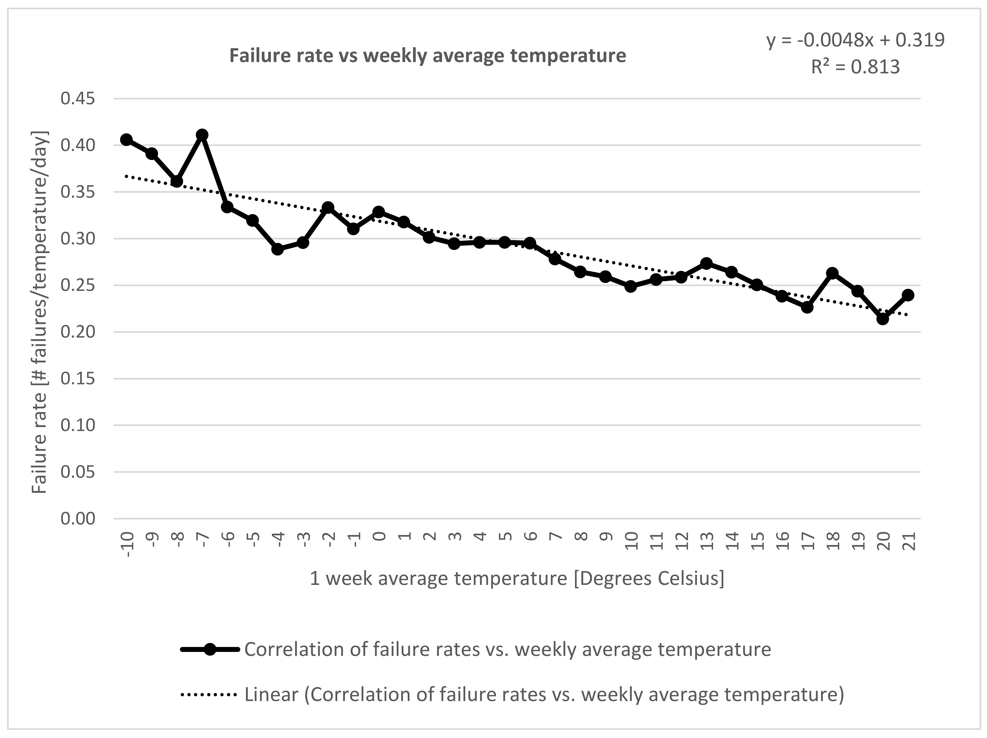
Figure 6 presents a plot of failure rates (failures/temperature/day) versus the average temperature of the preceding week. A linear correlation is plotted based on the data plots, with an accompanying equation and an R2 value. The linear regression shows a trend of an inverse correlation between increasing failure rates and weekly average temperatures, with a higher R2 value than the correlation of failure rates and temperature (calculated to be 0.782 in Section 3.1). This means that about 3% more of the variation in the data can be explained by the average weekly temperature than the temperature on the day of the failure.
Linear Regression Model
The regression line adapted with the least squares method has the following equation:
The slope is −0.0048 and the point of intersection is 0.319. There is a negative linear correlation between the failure rates and average weekly temperatures. The correlation coefficient R and the coefficient of determination R2 for the regression line is −0.901 and 0.813, respectively. In order to determine if there is statistically proof to state that there is a negative linear correlation between failure rates and average weekly temperatures, we performed a test of hypothesis according to the process described in Section 3.3.1. For the weekly temperature analysis, we put z = 30 since number of representative samples for weekly average temperature was n = 32. Calculating the test parameter t with n = 32, ρ0 = 0, and our R and R2 calculated values gave us a t = −11.54, which meant that we could reject the null hypothesis with a certainty of 99.9995% (a = 0.0005) and conclude that there is statistical evidence of a negative linear correlation.
3.5. Expected Impact of Climate Change on Reliability
The temperature increases that were used in the calculations for temperatures in 2070 for the three RCP scenarios are given in Table 1. The process described in Section 2.3 was used to calculate the values. The temperatures are averages calculated from the two downscaling processes described in Hanssen-Bauser et al. [2]. For expected temperature in 2070, the values in the table were added to the historical registered temperature range, based on a division of the seasons on temperatures, as described in Section 2.3, segment q. The temperature increases represent a national average and does not consider local differences, dependent on for example inland vs. sea locations, and north vs. south locations.
The process described in Section 2.4 was then used to calculate the expected increase or decrease in failures and failure rates in 2070. The results of these calculations are given in Table 2.
The calculations are based on the temperature vs. failure rate data since the situation becomes more diffuse when trying to predict a future change in weekly average temperatures. Sticking to a single temperature in this case makes it more straightforward to predict the future state. As can be seen from
Table 2, a reduction of 2.7% is expected in the ‘best case’ climate scenario, and a reduction of 7.2% in the ‘worst case’ climate scenario. It is, therefore, expected that a reduction in failures and failure rates will occur within 2070, and that this reduction is expected within the interval of 2.7 to 7.2%.
4. Discussion
The literature study has shown, that between the main climate change factors, temperature is singled out as a major contributor to water pipe failures. Several studies in the literature show the increase of failure rates during winter months. Frost loading of the pipes is indicated as a major driver for this increase. The literature also points to a correlation between grey cast iron pipes, frost loading, bending forces and transverse fractures. A large dataset of Norwegian failure data shows that 51% of total failures are transverse. Several studies found that transverse fractures happened mainly during winter months, thus supporting our hypothesis that frost loading is the main cause of transverse fractures, and thus a main cause for failures in general. Our study was based on this hypothesis, and one of the main drivers was to investigate the potential correlation between failures and temperature with a large failure dataset, and if found to be significant, quantify the correlation.
The main findings of the paper are twofold. First, it is the demonstrated correlation between temperature and failure rates, and weekly average temperature and failure rates. Both of them show a statistically significant correlation, with a bit stronger correlation model established between the latter variables than between the former. Both correlation calculations show a high degree of statistical significance (>99.999% certainty), with R2 values of 78.2% and 81.3%. The quantitative correlations that are defined by Equations (9) and (12) can thus be used to estimate failure rates and number of failures in a network based on air temperature levels. According to the linear correlation of temperature vs. failure rates, defined by Equation (9), the failure frequency (observed failures per day) is 86% higher at −15 degrees Celsius than at 23 degrees Celsius, and it is 52% higher at 0 degrees Celsius than at 23 degrees Celsius. This means that we are observing almost twice as many failures in the coldest part of the year as in the warmest part. According to the linear regression model of temperature vs. failure rates (Equation (9)) the failure frequency increases with 0.0235 for each 5 degree Celsius temperature increase, which equates to 0.047 for each 10 degree increase.
The second main finding is the future expected reduction in failure rates of drinking water pipes based on three climate scenarios defined in the national guideline for future climate change in Norway. The temperature correlation, instead of the weekly average temperature correlation, was used to calculate the future impact of temperature increase since this parameter is easier to estimate into the future. Rather unexpectedly, the long-term reliability of drinking water networks in cold climates can expect to be improved due to climate change. Increased temperatures correspond to a linearly reduced failure rate, proven by Figure 5 and Figure 6, and defined by Equations (9) and (12). The case study revolving around the extensive amount of failure data, specifically 25,573 recorded failures, have been able to quantify the impact of future climate scenario temperature increases on the failure rates. The expected decrease of future failure rates, as given in
Table 2, can be used to estimate future network reliability, and will help to assess future rehabilitation and investment needs. Many strategic rehabilitation planning tools rely on failure rates and failure data, among others WARP [26], PARMS [27] and KANEW [28]. The future expected reduction in failure rates can thus be used in conjunction with these programs in the future estimation of rehabilitation needs. We can expect a slightly reduced rehabilitation need in cold climate regions, since 2.7 to 7.2% of the expected failures within 2070 will be postponed. A natural consequence of the results is that the rehabilitation rates can be reduced with approximately 5% within 2070, depending on the climate change scenario outcome. It also means that investments can be postponed to a later timeframe, extending the lifetime expectancy of drinking water networks in cold climates. These conclusions naturally do assume that the service and risk level targets will be kept at current levels, and that operation and maintenance practices will be kept at status quo. Hydraulic reliability will also play a role when assessing necessary future rehabilitation rates. For example, population growth and urbanization can lead to hydraulic deficiency in some areas, leading to a need to upgrade the hydraulic capacity of the network. This is however outside the topic of this paper and will therefore not be looked further into.
Future scenario planning and extrapolation of data into the future is always associated with uncertainty. The uncertainty of the impact on failure rates is given within the range of the climate scenarios, as scenario planning tries to describe and embrace uncertainty instead of reducing it. This concept of scenarios can be described by a cone [29,30], where uncertainty increases with time and the worst and best case scenarios represent the outer limit of the cone. It is, therefore, reasonable to assume that the range of expected reduction of failure rates given in this paper are within reliable limits with regard to uncertainty. Outside of this uncertainty there are other factors which might affect the calculations. One of them is the expectation that extreme frost events might be worse due to climate change. This is highlighted in the literature study by the observation of increased movement of the northern polar vortex, causing extreme cold events in Northern America and Northern Europe. Accompanying this observation is associated extreme cold weather events in cold climates, which cause an increase in water main breaks. These instances have been reported in a number of newspaper articles in recent years. The question we ask is whether this phenomenon can counteract the positive effect of an increased average annual temperature on failure rates. We do to some degree argue that the temperature vs. failure rate correlation, as established in Section 3.3, does take the impact of extreme cold events into consideration since failure rates are highest with the coldest temperatures. In the assessment of future failure rates we do therefore assume that failures are higher for the coldest events, but we do not assume that a very limited amount of events will go outside of the correlation curve established by Equation (9). This is a topic which should be looked further into, and we can give no clear conclusion on this matter as per now.
The second factor, which might impact calculations, is the failure searching procedures within the municipalities, and practical circumstances like holidays. In order to show the potential impact of these circumstances, we will present two situations on opposite sides. First, some Norwegian municipalities focus on searching for failures and leakages in drinking water pipes during the spring to fall period, which means that the effort can somewhat be reduced in the winter. Such a practice can lead to a skewed distribution of failures across registration months since failures occurring in late winter months may not be registered until an extensive leakage reduction program is initiated in the early spring. This case can skewer the data in a way that falsely decreases failures for cold temperatures. Secondly, most operational crews take holidays during the summer, which means that extensive leakage reduction programs are more or less put on hold during the month of July, and also probably some of June and August. Many of the failures occurring during these months, which also are the hottest months, may therefore not be registered until early fall. This case can skewer the data in a way that falsely decrease failures for warm temperatures. It can then be discussed if these two cases somewhat nullify each other by skewering data in opposite directions. That is the first argument for stating that these cases may not impact the correlation results in a dire way, although the correctness of the correlation equations will be impacted to some extent. The second argument for stating that these cases may not be as influential on the results as feared is the massive amount of registrations used in the case study. The large amount of data will to a large degree help to even out the overall effect of such circumstances, as the skewering of data will be counteracted by the comprehensive amount of representative data.
5. Conclusions
This paper consists of a literature study on the impact of climate factors, most specifically temperature, on the structural reliability of drinking water pipes in cold climate regions. Some important conclusions can be drawn from this study:
- -
- Failure rates increase during cold winter months.
- -
- Frost loading and frost heave is an important factor for increased failure rates during winter months.
- -
- Changed soil temperatures cause thermal stresses in the ground, which impact pipes.
- -
- A large portion of failures in cold climates are transverse, which are normally caused by pipe-soil interactions and pipe bending.
- -
- Transverse fractures can be doubled during winter months.
- -
- Pipes in trenches which are more vulnerable to frost heave experience more failures during winter than the average of the network, thus verifying the frost heave effect on pipes during winter.
- -
- Grey cast iron pipes are more vulnerable to failures during winter months than other materials, being the only material that has a substantially increased failure rate during winter months. These pipes are also often laid in trenches exposed to frost heave (certain construction periods), showing that there might be a connection between high failure rates of grey cast iron pipes and frost vulnerable construction periods.
The empirically-based data study performed in the paper, the literature study, and the real world observations reported in several newspaper articles confirm that failures occur more often during the colder winter months than during the warmer summer months, and that extreme cold weather intensifies the failure occurrences. This paper has produced a statistically significant correlation between failure rates and temperatures, and between failure rates and average weekly temperatures. The correlations show that failures will occur with a higher rate in cold weather months than in warm weather months, resulting in a higher occurrence of failures on cold days than on days with warm weather. As an illustration of the impact of temperature, failures occur 86% more often in −15 degrees Celsius than in 23 degrees, which means that we are observing almost twice as many failures in the coldest part of the year as in the warmest part. According to the linear regression model of temperature vs. failure rates, the failure frequency increases with 0.047 for each 10 degrees increase.
The correlation model of failure rates vs. weekly temperature has a barely higher R2 value than the model for correlation of failure rates vs. temperature, showing a slightly stronger explanation of the variation in the data. The difference in R2 value is 0.03. We therefore conclude that 3% more of the variation in data can be explained by weekly average temperatures than by daily temperatures. This also shows us that failure rates are more dependent on type of season (cold vs. warm season) than the length of the cold period. A general conclusion is that the frequency of a failure event increases drastically in cold weather/cold seasons, and that the length of a cold period within the season further increases the frequency of an event, although in a small measure.
Furthermore, the correlation calculations have been used together with future climate prediction data to estimate a change in failure rates within 2070. A national guideline for future climate change in Norway has been used to predict temperature increases for the different seasons within 2070, based on different climate change scenarios. These estimations have been used together with historical climate data to predict actual temperatures through the seasons in 2070. These estimated temperatures have then been coupled to historical data on temperatures vs. failure rates, in order to predict a change in failure rates within 2070. The analysis shows that we can expect a decrease in failure rates in the range of 2.7 to 7.2% due to temperature changes. We therefore conclude that the structural reliability of drinking water networks in cold climates will be improved within 2070 due to climate change. We recommend using an expected reduction of failure rates in the range of 5% (most probable scenario outcome shows a reduction of 4.4%) when planning future rehabilitation needs. This will have the beneficial effect of increased average lifetime expectancy of networks and a postponement of some investments.
The paper has shown to contribute to current state of the art by quantifying the correlation between failure rates and temperature. Equation (9) can be used by utilities in cold climates to estimate failure occurrences in their networks based on weather forecasts or to estimate expected changes in future failure rates based on climate scenarios down scaled to local situations. The paper has further added to current state of the art by estimating future expected decrease in failure rates based on Norwegian climate scenarios. The changes in future failure rates for any utility in cold climate regions can be estimated locally based on local down scaled climate scenarios, or the estimations found in this paper can be used if no downscaled scenarios are available. These two contributions to state of the art is considered to cover current research gaps on the topics.
Acknowledgments
The authors would like to thank the municipalities in the VASK group in Norway, the Norwegian interest group for water ‘Norsk Vann’, and the Norwegian Research Council (Grant number 243497) for the financing and support of this work. The Norwegian University of Science and Technology has financed the open access fee of the paper.
Author Contributions
Stian Bruaset conceived the method, gathered data, made the calculations and wrote the paper. Sveinung Sægrov contributed to the overall content of the paper through discussions, feedback and guidance, and through specific feedback on the writing of the paper.
Conflicts of Interest
The authors declare no conflict of interest.
References
- Ugarelli, R.; Leitão, J.P.; Almeida, M.C.; Bruaset, S. Overview of climate change effects which may impact the urban water cycle—D2.2.1. In European Union Seventh Framework Programme; European Union: Brussels, Belgium, 2010. [Google Scholar]
- Hanssen-Bauer, I.; Førland, E.J.; Haddeland, I.; Hisdal, H.; Mayer, S.; Nesje, A.; Nilsen, J.E.; Sandven, S.; Sandø, A.B.; Sorteberg, A.; et al. Klima i Norge 2100. Kunnskapsgrunnlag for Klimatilpasning Oppdatert i 2015—NCCS Report No. 2; Miljødirektoratet: Oslo, Norway, 2015. [Google Scholar]
- James, T. Cold Snap Led to Daily Water Main Breaks, City Says. Saskatoon StarPhoenix. 2017. Available online: http://thestarphoenix.com/news/local-news/cold-snap-led-to-daily-water-main-breaks-city-says (accessed on 15 January 2018).
- Wood, P.; Wells, C. Cold Snap Is Snapping Water Pipes in City, Counties. The Baltimore Sun. 2015. Available online: http://www.baltimoresun.com/news/weather/weather-blog/bs-md-cold-problems-20150217-story.html (accessed on 15 January 2018).
- Winters, C. Cold Snap Causes 3rd Everett Water Main to Break. HeraldNet. 2017. Available online: http://www.heraldnet.com/news/cold-snap-causes-3rd-everett-water-main-to-break/ (accessed on 18 January 2018).
- Sobel, A. Record Cold Does not Disprove Global Warming. 2014. Available online: http://edition.cnn.com/2014/01/07/opinion/sobel-winter-cold-global-warming/ (accessed on 17 April 2015).
- Walsh, B. Climate Change Might Just Be Driving the Historic Cold Snap. 2014. Available online: http://science.time.com/2014/01/06/climate-change-driving-cold-weather/ (accessed on 17 April 2015).
- NASA. Polar Vortex Enters Northern U.S. 2014. Available online: http://www.nasa.gov/content/goddard/polar-vortex-enters-northern-us/#.Usyt2iiyVcg (accessed on 17 April 2015).
- Brekke, K.; Husebø, G. Snart Vannkrise. 2006. Available online: http://www.nrk.no/hordaland/vannkrise-i-bergen-1.373274 (accessed on 20 April 2015).
- Herseth, S.K. Nå er det Vannkrise i Bergen. 2010. Available online: http://www.dagbladet.no/2010/02/16/nyheter/innenriks/vann/bronner/10421383/ (accessed on 20 April 2015).
- Intergovernmental Panel on Climate Change—IPCC. Climate Change 2014 Synthesis Report. 2014: Contribution of Working Groups, I.; II and III to the Fifth Assessment Report of the Intergovernmental Panel on Climate Change; Core Writing Team, Pachauri, R.K., Meyer, L.A., Eds.; IPCC: Geneva, Switzerland, 2014. [Google Scholar]
- Meteorologisk Institutt. Klima Siste 150 år. 2010. Available online: http://met.no/Klima/Klimautvikling/Klima_siste_150_ar/ (accessed on 17 April 2015).
- Meteorologisk Institutt. Norge fra 1900 til i dag—Temperatur. 2014. Available online: http://met.no/Klima/Klimautvikling/Klima_siste_150_ar/Hele_landet/ (accessed on 17 April 2015).
- Meteorologisk Institutt. Temperaturavvik fra normal Norge—Vinter. 2015. Available online: http://eklima.met.no/metno/trend/TAMA_G0_24_1000_NO.jpg (accessed on 17 April 2015).
- Vreeburg, J.; Vloerbergh, I.N.; Van Thienen, P.; De Bont, R. Shared failure data for strategic asset management. Water Sci. Technol. Water Supply 2013, 13, 1154–1160. [Google Scholar] [CrossRef]
- Kutyłowska, M.; Hotloś, H. Failure analysis of water supply system in the Polish city of Głogów. Eng. Fail. Anal. 2014, 41, 23–29. [Google Scholar] [CrossRef]
- Rajani, B.; Zhan, C.; Kuraoka, S. Pipe soil interaction analysis of jointed water mains. Can. Geotech. J. 1996, 33, 393–404. [Google Scholar] [CrossRef]
- Makar, J. Failure analysis for grey cast iron water pipes. In Proceedings of the AWWA Distribution System Symposium; AWWA—American Water Works Association: Reno, NV, USA, 1999. [Google Scholar]
- Reikvam, S. Cold Induced Damages on Water Pipelines; Master Thesis at Norwegian University of Science and Technology: Trondheim, Norway, 2013. [Google Scholar]
- Le Gauffre, P.; Aubin, J.-B.; Bruaset, S.; Ugarelli, R.; Benoit, C.; Trivisonno, F.; Van den Bliek, K. Deliverable 5.5.4. Impacts of climate change on maintenance activities: A case study on water pipe breaks. European Union 7th Framework Project PREPARED. Available online: http://www.prepared-fp7.eu/viewer/file.aspx?FileInfoID=443 (accessed on 31 March 2018).
- Wu, Y.; Sheng, Y.; Wang, Y.; Jin, H.; Chen, W. Stresses and deformations in a buried oil pipeline subject to differential frost heave in permafrost regions. Cold Reg. Sci. Technol. 2010, 64, 256–261. [Google Scholar] [CrossRef]
- Xu, G.; Qi, J.; Jin, H. Model test study on influence of freezing and thawing on the crude oil pipeline in cold regions. Cold Reg. Sci. Technol. 2010, 64, 262–270. [Google Scholar] [CrossRef]
- Jin, H. Design and Construction of a Large-Diameter Crude Oil Pipeline in Northeastern China: A Special Issue on Permafrost Pipeline; Elsevier: Amsterdam, The Netherlands, 2010. [Google Scholar]
- Makar, J.; Desnoyers, R.; McDonald, S. Failure modes and mechanisms in gray cast iron pipe. In Underground Infrastructure Research; CRC Press: Boca Raton, FL, USA, 2001; pp. 1–10. [Google Scholar]
- Helbæk, M. Statistikk—Kort og Godt; Universitetsforlaget: Oslo, Norway, 2011. [Google Scholar]
- Rajani, B.; Kleiner, Y. WARP-water mains renewal planner. In Proceedings of the International Conference on Underground Infrastructure Research, Waterloo, ON, Canada, 10–13 June 2001. [Google Scholar]
- Burn, S.; Tucker, S.; Rahilly, M.; Davis, P.; Jarrett, R.; Po, M. Asset planning for water reticulation systems-the PARMS model. Water Sci. Technol. Water Supply 2003, 3, 55–62. [Google Scholar]
- Herz, R.K. Software for Strategic Network Rehabilitation and Investment Planning; Water Intelligence Online: London, UK, 2003. [Google Scholar]
- Galloway, G.E. If Stationarity Is Dead, What Do We Do Now? Wiley Online Library: Hoboken, NJ, USA, 2011. [Google Scholar]
- Waage, M. Nonstationarity Water Planning Methods. In Proceedings of the Workshop on Nonstationarity, Hydrologic Frequency Analysis, and Water Management, Boulder, CO, USA, 13–15 January 2010. [Google Scholar]
Figure 1.
Overview of the method used to assess potential impact of future temperature change on failure rates.
Figure 1.
Overview of the method used to assess potential impact of future temperature change on failure rates.
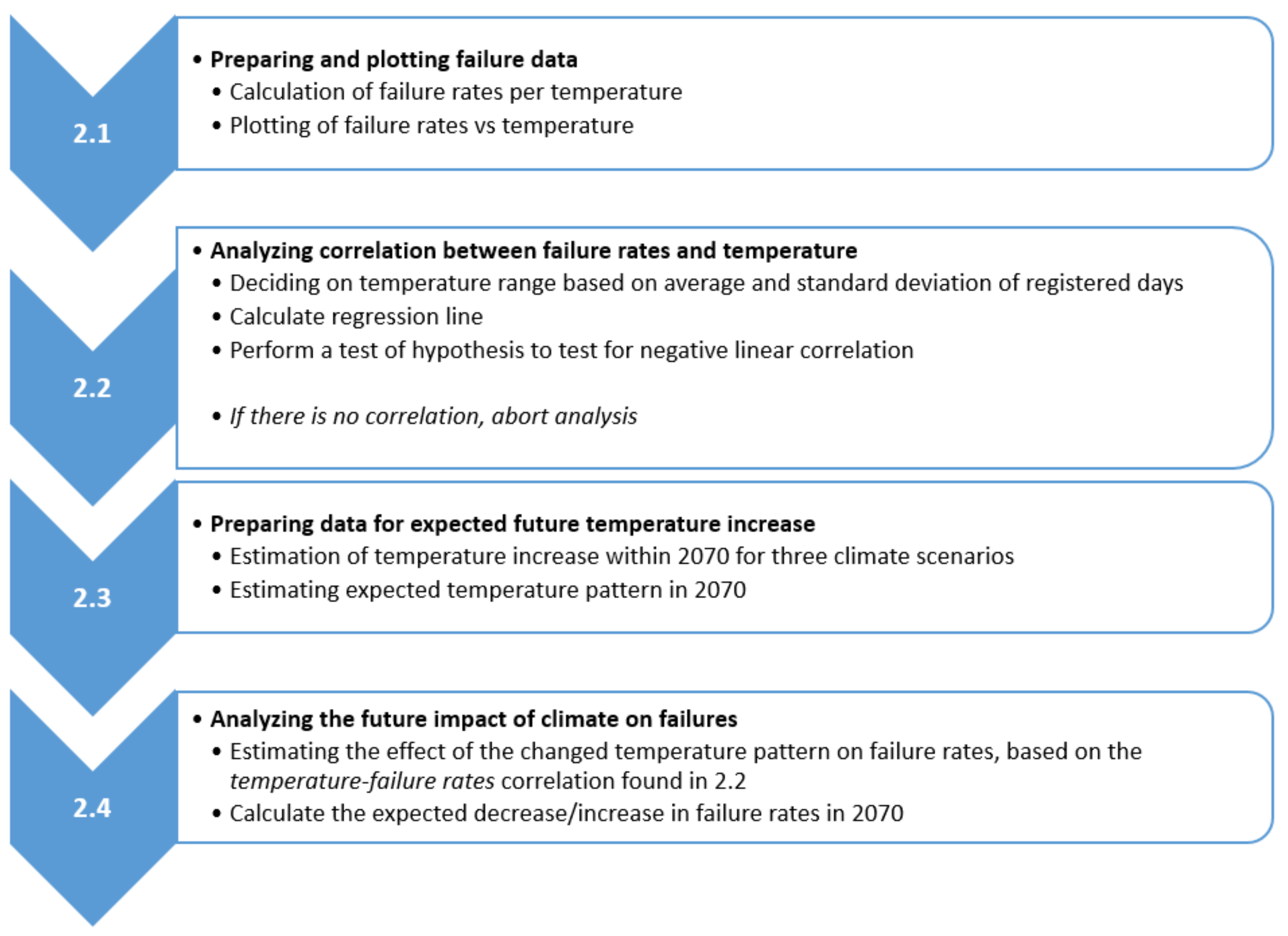
Figure 2.
An illustration of data used to predict future impact of temperature increase on failures.
Figure 2.
An illustration of data used to predict future impact of temperature increase on failures.
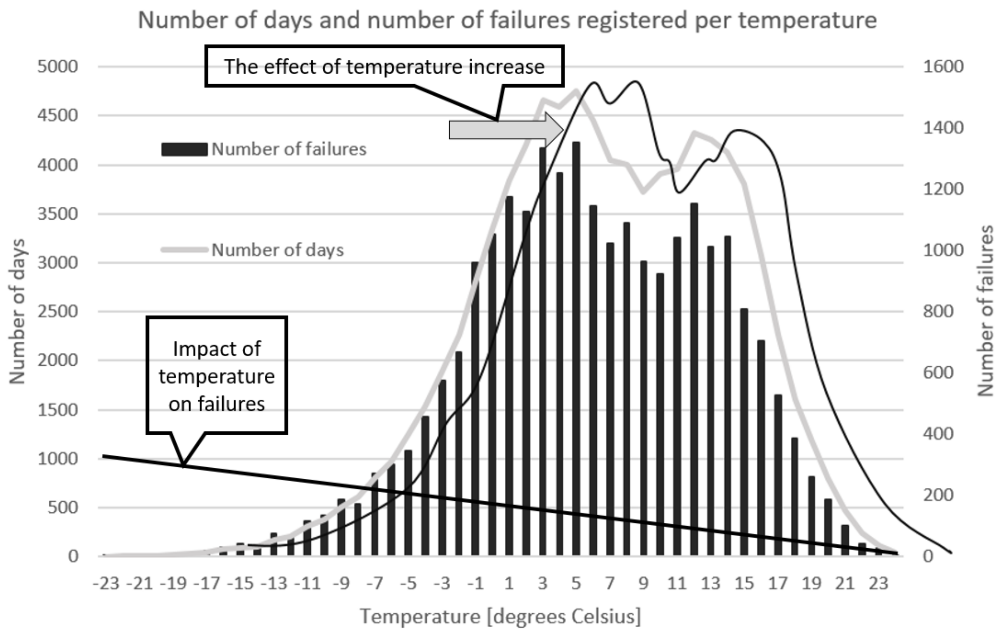
Figure 3.
Number of failures correlated against diameter of pipes.

Figure 4.
Number of failures correlated against construction year of pipes.
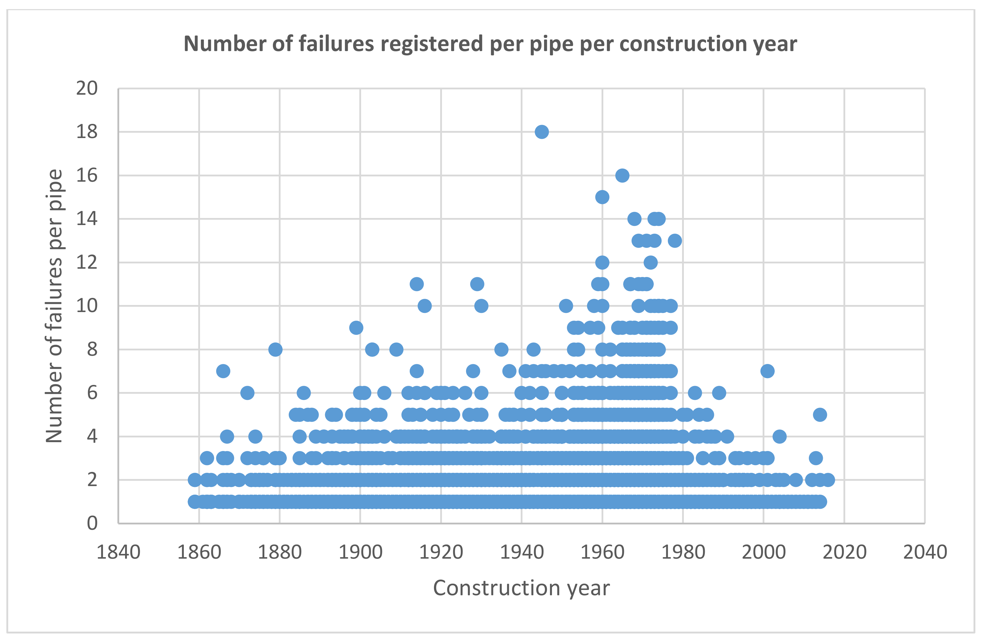
Figure 5.
Linear regression showing the correlation between failure rates and temperature.
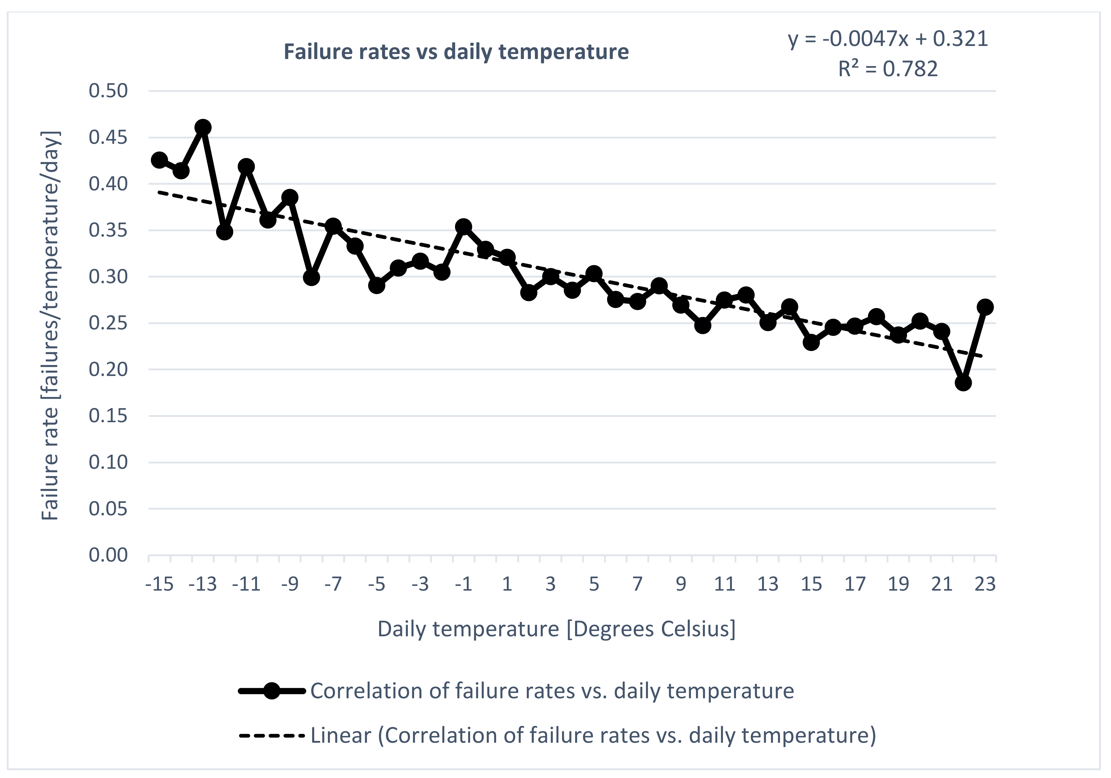
Figure 6.
Linear regression showing the correlation between failure rates and average temperature the preceding week.
Figure 6.
Linear regression showing the correlation between failure rates and average temperature the preceding week.


Table 1.
Expected temperature increase used in the three scenarios, distributed across the three seasons. The numbers are based on calculations in Hanssen-Bauer et al. [2].
Table 1.
Expected temperature increase used in the three scenarios, distributed across the three seasons. The numbers are based on calculations in Hanssen-Bauer et al. [2].
| Temperature Increase [Degree C] | RCP Scenarios | ||
|---|---|---|---|
| Season | RCP 2.6 | RCP 4.5 | RCP 8.5 |
| Winter | 1.9 | 3.1 | 5.35 |
| Fall + spring | 1.9 | 2.95 | 4.6 |
| Summer | 0.7 | 2.0 | 3.4 |
Table 2.
Expected change in number of failures/failure rates within 2070 due to temperature increase. The change is given in % compared to historical failure data.
Table 2.
Expected change in number of failures/failure rates within 2070 due to temperature increase. The change is given in % compared to historical failure data.
| Scenario | RCP 2.6 | RCP 4.5 | RCP 8.5 |
|---|---|---|---|
| % change | −2.7 | −4.4 | −7.2 |
© 2018 by the authors. Licensee MDPI, Basel, Switzerland. This article is an open access article distributed under the terms and conditions of the Creative Commons Attribution (CC BY) license (http://creativecommons.org/licenses/by/4.0/).
Share and Cite
MDPI and ACS Style
Bruaset, S.; Sægrov, S. An Analysis of the Potential Impact of Climate Change on the Structural Reliability of Drinking Water Pipes in Cold Climate Regions. Water 2018, 10, 411. https://doi.org/10.3390/w10040411
AMA Style
Bruaset S, Sægrov S. An Analysis of the Potential Impact of Climate Change on the Structural Reliability of Drinking Water Pipes in Cold Climate Regions. Water. 2018; 10(4):411. https://doi.org/10.3390/w10040411
Chicago/Turabian StyleBruaset, Stian, and Sveinung Sægrov. 2018. "An Analysis of the Potential Impact of Climate Change on the Structural Reliability of Drinking Water Pipes in Cold Climate Regions" Water 10, no. 4: 411. https://doi.org/10.3390/w10040411
Note that from the first issue of 2016, this journal uses article numbers instead of page numbers. See further details here.