Identification of Factors That Influence Energy Performance in Water Distribution System Mains

Jacobs Engineering, Toronto, ON M2J 1R3, Canada 2 Civil Engineering Department, Queen’s University, Kingston, ON K7L 3N6, Canada
*
Author to whom correspondence should be addressed.
Water 2018, 10(4), 428; https://doi.org/10.3390/w10040428
Submission received: 9 March 2018
/
Revised: 28 March 2018
/
Accepted: 3 April 2018
/
Published: 4 April 2018
(This article belongs to the Special Issue Energy and Water Sustainability: Energy Supplies in Water Exploration, Production and Delivery)
Abstract
:This paper aims at identifying paramount hydraulic factors in energy dynamics of water mains, using Principal Components Analysis (PCA). The proposed method is applied to two large ensembles of leaky and non-leaky pipes comprising over 40,000 pipes selected from 18 North American water distribution systems to guarantee the versatility of pipe characteristics and statistical significance of the explored patterns. PCA mono-plots indicate energy metrics such as Net Energy Efficiency, Energy Lost to Friction and Energy Lost to Leakage serve better in identification of low from high efficiency pipes. In addition, PCA mono-plots and bi-plots reveal relative importance of hydraulic parameters and that average flow rate, hydraulic proximity to major components and average unit headloss can have more tangible effects on energy dynamics of pipes compared to leakage and average pressure. Some factors such as elevation, diameter and CHW are not as influential as expected in distinguishing high-efficiency from low-efficiency pipes. Further, a comparison between the approach used in this paper and a simplified common-practice replacement strategy points out the difference energy considerations can make, if included in a bigger asset management landscape.
1. Introduction
Water main aging and deterioration tends to evolve in lockstep with a loss of hydraulic capacity, an increased leakage, and a higher pumping energy requirement in a water distribution system [1,2,3,4,5]. There are several factors such as operating pressure and topographical elevation that are known to have a large impact on the energy performance of water mains and water distribution systems in general [6]. Often, detailed hydraulic modeling and/or optimization are needed to fully ascertain the extent to which changes in hydraulic parameters will change the energy use in distribution systems. Unfortunately, advanced energy modeling and optimization are not extensively used in engineering practice nor do most water utilities have the resources to perform these analyses to characterize the energy performance of their systems. Further, the large number of variables in distribution system operation is an important barrier that makes it difficult for water utility managers to gain a clear picture of how system operations and the state of deterioration of pipes act together to affect the energy performance of water mains and their systems.
Previous studies that have considered energy issues in distribution systems have only examined a few case study systems in an ad hoc fashion. Energy indicators to relate system-wide energy efficiency to pump efficiency and reservoir location were developed, without considering leakage impacts [7]. Cabrera et al. [8] presented a set of metrics to characterize the system-wide energy performance that includes losses to friction, leakage, and overpressure. These energy metrics provided a useful set of tools to help water utility managers better understand how far their systems were from an ideal energy-efficient state but fall short of being able to identify individual pipes that would be problematic. Building upon their earlier work, the same authors presented additional metrics to assess the energy efficiency of a pressurized system and procedures to prioritize interventions on a system-wide basis [9]. The study [10] examined the energy dynamics of groups of pipes and pumps in the Toronto distribution system. While these researchers also solved the energy balance to examine the frictional losses in individual pipes of the Toronto system, they did not examine the efficiency, leakage, and other energy characteristics of these pipes. The results of these previous studies pertain specifically to the specific distribution systems examined and it is an open question as to whether these results are transferrable to a wide cross section of real, complex systems.
To address this problem, this research focuses on applying the tools of statistical analysis to large datasets spanning multiple systems to examine the relationships between pipe and hydraulic parameters and energy performance. What motivates the use of large datasets and this statistical approach is that the ensuing results have statistical significance and are transferrable across a wide cross section of large, complex distribution systems [11]. The knowledge gleaned from this research can be used by water utilities to identify water main assets with threshold levels that lead to low energy performance without having to resort to advanced water distribution and energy modeling and optimization techniques.
The aim of this paper is to build on the work of Hashemi et al. [11] to identify the hydraulic parameters that have the largest impact on the energy performance of water main assets in distribution systems. The paper answers three research questions:
- What hydraulic parameters have the largest influence on the energy performance for water mains data in distribution systems?
- What combinations of hydraulic parameters can better distinguish highly efficient water mains from those with low efficiency?
- How aligned are the simplified rehabilitation approaches, for example those based on pipe age or break rate, with energy efficiency in water mains?
A statistical approach is taken to address these three research questions. This paper applies principal components analysis (PCA) to an ensemble of 40,000 water mains across 18 water distribution systems. The choice to use PCA in this paper is motivated by two challenges: First, the high dimensionality (numerous pipe and hydraulic parameters) of the dataset makes it difficult to visualize and identify what parameters drive energy use. Second, the dataset comprises 40,000 data points (40,000 water mains across 18 systems) so the large number of data points requires advanced statistical techniques to fully explore [2,3]. PCA is a proven technique that can simplify a large dataset and identify the most influential parameters that drive energy use in distribution systems. Thus far, there has been little research that has deployed statistical techniques like PCA to examine the energy dynamics of water mains with a large set of data on pipes across numerous systems.
The new knowledge created in this paper has the potential to help water utilities perform a screening-level identification of groups of pipes that are likely to have a low energy performance and follow up with targeted condition assessment and hydraulic modeling to further examine the energy performance of pipes and their candidacy for rehabilitation.
2. Methods
2.1. Pipe-Level Energy Metrics
The pipe-level energy metrics developed by the authors [12] were used in conjunction with PCA to examine the relationship between pipe and hydraulic parameters (e.g., average flow (Ave Q), pipe roughness (CHW), pipe diameter (D), average unit headloss (UH), presssure (P), elevation (Elv) and hydraulic proximity to major components) and energy use in water mains of distribution systems (see Table 1). The pipe-level metrics and their parameters are defined in Equations (1)–(6). The reader can refer to [12] to obtain more details on these pipe-level metrics.
where GEE, the gross energy efficiency (Equation (1)), compares the energy delivered to the users serviced by a pipe (Edelivered) to the energy supplied to that pipe (Esupplied). Each energy components are defined in Table 1. NEE, net energy efficiency (Equation (2)), compares the energy delivered to users serviced by a pipe (Edelivered) to the net energy in that pipe (Esupplied − Eds), where net energy is the energy supplied to the pipe minus (Esupplied) the energy supplied to users located downstream of the pipe and not directly serviced by the pipe (Eds). ENU, energy need by user (Equation (3)), compares the energy delivered to the users serviced by a pipe (Edelivered) against the minimum energy needed by those users (Eneed). The minimum energy by a user is defined as Eneed = γ Qmin Hmin Δt and is a function of the minimum water use needed by users (Qmin) and the minimum pressure head required to deliver acceptable water service to users (Hmin). ELTF, energy lost to friction (Equation (4)), compares the magnitude of friction loss in the pipe (Efriction to satisfy the demand and leakage at the end of the pipe, and demands downstream of the pipe) to the net energy supplied to the pipe (Esupplied − Eds). ELTL, energy lost to leakage (Equation (5)), compares the sum of the energy lost directly to leakage and the frictional energy loss along the pipe required to meet the leakage flow, Ql, at the end of the pipe or Eleak + Efriction (leak) relative to the net energy supplied to the pipe.
2.2. Principal Components Analysis (PCA)
The multivariate analysis of a considerable number of energy indicators and hydraulic factors (a high-dimensional problem) makes PCA a pertinent tool to reduce the dimensionality of a dataset. Using PCA makes it possible to identify what parameters account for most of the variance and scatter in the original dataset [13,14]. In this way, PCA makes it possible to visualize a large dataset and identify what pipes and groups of pipes possess combinations of characteristics that lead to low energy performance.
PCA essentially builds on a correlation matrix to visualize and explore patterns or relationships not captured by correlation analysis. Principal Components (PCs) are linear combination of Eigenvalues of the correlation matrix of the statistical ranks of hydraulic parameters and energy metrics [11]. They are, therefore, orthogonal and not correlated. Each data point (pipe) will be assigned a score on the PCs, hence the dataset along these PCs shows the most variance/scatter. This will distinguish pipes or groups of pipes from each other as the point of interest in this paper. The first few PCs, corresponding to the larger Eigenvalues of the correlation matrix, describe most of the variance in the dataset and are statistically sufficient to describe the variance of the data.
PCA Mono-Plots and Bi-Plots
A “mono-plot” is the representation of the hydraulic factors and energy metrics on the orthogonal axes of the first two PCs. Hydraulic factors or energy metrics with high scores on either axes of the mono-plot tend to be more influential on the variance of the dataset. Parameters that track closely together have similar effects on the dataset, while parameters that diverge from one another have a different influence on the dataset. Moreover, the original observations in the dataset can be presented in a “bi-plot” by transforming their original values into new PC coordinates, as described in Equation (6):
where (pipei score)j is the score of pipei on the jth PC, [pipei]1×n is the vector on the ith row on the matrix of pipes including the ranks of all n hydraulic variable values for pipei and [PCj]n×j is the Eigenvector corresponding to the jth largest Eigenvalue (the jth PC), including the scores of all n hydraulic parameters. Therefore, each pipe or observation will be assigned one value on each of the new directions or PCs, which makes the visualization of the observation on the new/transformed coordinate system possible. Clusters of pipe scores on the PCA bi-plot can distinguish data groups with similar characteristics. The formation of clusters can help identify the factors that have the most impact on the similarities or dissimilarities in the observations.
3. Application of Multivariate Statistical Analyses in Large WDSs
To yield robust results in statistical analysis, this paper required a benchmarking dataset representative of the wide variety of characteristics such as configuration, pipe conditions and age profile, found in different water distribution systems. Eighteen distribution networks, therefore, were selected from different areas in the states of Kentucky and Ohio in the United States as well as the province of Ontario in Canada [15,16,17]. The network models in Ohio and Ontario are those utilized by corresponding municipalities while Kentucky models comprise a database developed from GIS files obtained from the Kentucky Infrastructure Authority [15]. This large dataset includes over 40,000 pipes. Seventeen of these systems comprise almost 20,000 pipes without information available on leakage (the non-leaky ensemble), while one system comprises approximately 20,000 pipes that include leakage for each pipe as estimated by a robust field measurement campaign (the leaky ensemble). It is noted that there might be background leakage or leakage included as a part of the demand for the non-leaky ensemble, however, not included as a separate factor. The results of multivariate statistical analyses of the networks with and without leakage were also juxtaposed to understand the importance of considering leakage in the energy dynamics of WDSs. The characteristics of these WDSs are summarized in Table 2. To obtain hydraulic outputs of the distribution systems (such as nodal pressures and pipe flows), EPANET2.0 network models were used [18]. EPANET2.0 hydraulic outputs were then retrieved by a code in Visual Basic 6.0 to evaluate energy metrics. Except for average pressure that is a hydraulic output by EPANET2.0, all other hydraulic characteristics of the systems in Table 2, such as water demand, pipe roughness and sizes, leakage, etc., are surveyed data and input to the hydraulic models. Lastly, Matlab R15 was used to perform matrix algebra calculations to obtain mono-plots and bi-plots [19].
4. Results
4.1. Hierarchical Importance of Parameters in Energy-Based Decision Making
4.1.1. Non-Leaky Ensemble
PCA for non-leaky systems includes 11 variables, including both hydraulic parameters as well as energy metrics, summarized in correlation matrix (Table 3). Figure 1 indicates the corresponding contribution of each PC, based on the 11 Eigenvalues of the correlation matrix in Table 3. According to Figure 1, in the non-leaky ensemble, the first two PCs describe almost 65% of the variance in the data (47.3% and 16.9%, respectively), while the other nine PCs account for 35% of the variance in the data. Hence, the first two PCs are selected to compress and visualize the pipe dataset in a two-dimensional space. It is noted that the PCs do not directly correspond to the parameters and variables in the correlation matrix of Table 3 and are linear combinations of them to introduce new directions on which the correlation is minimized and variance maximized.
The mono-plots presented in the next section are a visual expression of the importance of hydraulic parameters and metrics with regard to the first two PCs in both non-leaky and leaky (in a similar fashion) ensembles. Figure 2 shows the mono-plot for the non-leaky ensemble. The x-axis represents PC1, describing the most variation in the pipe dataset (47.3%). The y-axis represents PC2, describing the second most variation in the data (16.9%). More influential parameters and metrics are mainly perceived to have scores higher than 0.3 on each PC. However, to narrow down the important parameters and metrics for decision making, higher alignment with the PCs will also be preferable. According to Figure 2, GEE and NEE track closely, meaning that higher values for one result in higher values for the other as well. The PC1 values for these two metrics suggest that they are more influential in describing variance than parameters such as CHW, diameter and Elv. On the other hand, ELTF, Average flow (Ave. Q), headloss and proximity are clustered together. This not only means that they have similar effects on pipes, but also that high values of these parameters result in lower values of GEE and NEE. It is also noted that all parameters of GEE, NEE, ELTF, proximity, Ave Q and headloss are well represented with regard to PC1, as their respective vectors are first, much larger compared to parameters such as CHW and diameter and, second, closely aligned with the PC1 axis.
Moreover, along the PC2 axis, ENU and Pressure (P) are clustered together and have high vector magnitudes compared to other parameters. Therefore, it can be inferred that these two vectors are highly correlated/aligned to each other, and that they have higher importance compared to D and CHW. However, ENU and P have lower importance or influence compared to those with higher values along the PC1 axis (ELTF, GEE, NEE, headloss, etc.). This is mainly because PC2 describe less variance (16.9%) compared to PC1 (47.3%).
The CHW and D vectors are not situated close to any other parameters or to each other, which means that they will not affect the dataset in the same way as the other parameter. In addition, these vectors are not well represented on either the PC1 or PC2 axes, both in their magnitude and in their direction, which explains less importance in the variance of the ensemble. The Elv vector points away from other parameters, implying that it has a different effect on the variance of the pipe dataset. It can also be inferred that higher elevations cause lower pressure, since the Elv and P vectors point in opposite directions.
The Ave Q and unit headloss vectors point in a similar direction and in the opposite direction of the GEE and NEE vectors. From a hydraulic standpoint, this implies that an increase in Ave Q and/or unit headloss in a pipe causes a decrease in GEE, NEE. Moreover, P closely tracks with ENU, confirming that pressure directly influences energy surplus or deficit in a pipe. The correlation matrix in Table 3 also indicates no relationship between these two groups of parameters, supporting the results shown in Figure 2, where the two groups (P and ENU versus GEE, NEE and Ave Q) do not track closely.
4.1.2. Leaky Ensemble
Figure 3 shows the mono-plot for the leaky ensemble (indicated as system OH2 in Table 2 as the largest distribution network). PCA for this includes the same variables as in the non-leaky ensemble plus daily leakage and ELTL, which comes to the total of 13 variables as opposed to 11 in the non-leaky ensemble. Even though the percentage of leakage in this system is fairly small (almost 8%), Figure 3 shows slightly different results to those of Figure 2 which could illustrate the importance of considering leakage. As shown by the axes, PC1 describes 36.5% and PC2 20% of the variance. The sum of these contributions is slightly smaller compared to that of the previous mono-plot mainly because more parameters (including daily leakage and ELTL) are now included in the PCA, which makes each parameter less descriptive with regard to the total variance in the ensemble. According to Figure 3, influential parameters are GEE, ELTF, proximity, Ave Q and headloss as they all hold comparatively higher scores along PC1 (above absolute values of over 0.3 on both axes). Diameter is now more influential and closer to the cluster of ELTF, headloss, proximity, and Ave Q compare to the non-leaky ensemble results. This difference in the relative importance of the parameters may emphasize the importance of considering leakage and larger networks. Further, ELTL, leakage and NEE are the next most influential vectors, with high PC2 scores (absolute value over 0.40). Elv in the leaky ensemble is a fairly important parameter compared to CHW, pressure, and even ENU, because of the length of the corresponding vector in Figure 3. As in the results for the non-leaky ensemble, CHW is a less important parameter—its vector points away from other parameters and has a small magnitude. Compared to the non-leaky ensemble, although ENU and P still track closely, their importance is dwarfed by ELTL and leakage along the PC2 axis. This implies that in systems with leakage, the impact of pressure may be lower compared to leakage on the energy dynamics of the system.
Another noticeable difference from the non-leaky ensemble is that the NEE vector direction does not match those of other parameters. This could be due to considering leakage, meaning that NEE seems to be affected by two sources of inefficiency, leakage and friction. This can explain why NEE and GEE do not cluster together as they did in the non-leaky ensemble results. In general, considering leakage in the analysis seems to have shuffled the importance of some of the hydraulic parameters, even though there are still similarities between the two cases.
For the leaky case, diameter now seems to have gained more influence (with a score of −0.3 on PC1). It is also observed that average unit headloss and diameter can potentially have similar effects on the dataset, which was not captured originally by correlation analysis. It could also be interpreted as larger pipes being generally located near the major components, and thus may bear inherently higher unit headloss rates. This is also corroborated by the fact that water main sizes decrease moving away from major components in a system.
4.2. Clusters of High Efficiency Versus Low Efficiency Pipes
Results in Figure 2 and Figure 3 explain that of all the variables included in PCA, comparatively energy dynamics have higher importance in describing the variance in both ensembles, as they are expressed through longer vectors and highly aligned with PC1 and PC2 axes. This would suggest that the mono-plots represent energy dynamics landscape in the two ensembles. Therefore, the energy metrics values can be used to characterize high/low-efficiency pipes throughout the whole dataset.
To find clusters of high-efficiency pipes in the non-leaky and leaky ensembles, the corresponding threshold as to distinguish these pipes ought to be defined. Investigation on the relationship between the energy metrics values and common-practice thresholds by Hashemi et al. [11] indicate that, for the efficiency metric, NEE, values above 70th percentile of the data set correspond to high efficiency (NEE > 99.9%). Similarly, energy loss metric ELTF values below 30th percentile correspond to low efficiency pipes (ELTF < 0.0018%). Moreover, 100% < ENU < 105% correspond to the optimal pressure range (approximately 30–50 m) specified in North American guidelines [20,21,22]. In a similar way, for the other efficiency and energy loss metrics (GEE and ELTL), it is assumed that the same thresholds suffice to distinguish high efficiency pipes. Therefore, GEE > 20% and ELTL < 0.8% are considered highly efficient [11,23,24]. Based on the same investigations, low efficiency pipes are considered to have metric values below 30th percentile for GEE and NEE and above 70th percentile for ELEF and ELTL. ENU values corresponding to excessive pressure in pipes indicated by standard (approximately 70 m) are considered to indicate low efficiency pipes for this metric. Therefore, GEE < 15%, NEE < 99.4%, ENU > 113%, ELTF > 0.3% and ELTL > 3% indicate low-efficiency pipes. The threshold values considered for both non-leaky and leaky ensembles are summarized in Table 4.
4.2.1. Non-Leaky Ensemble
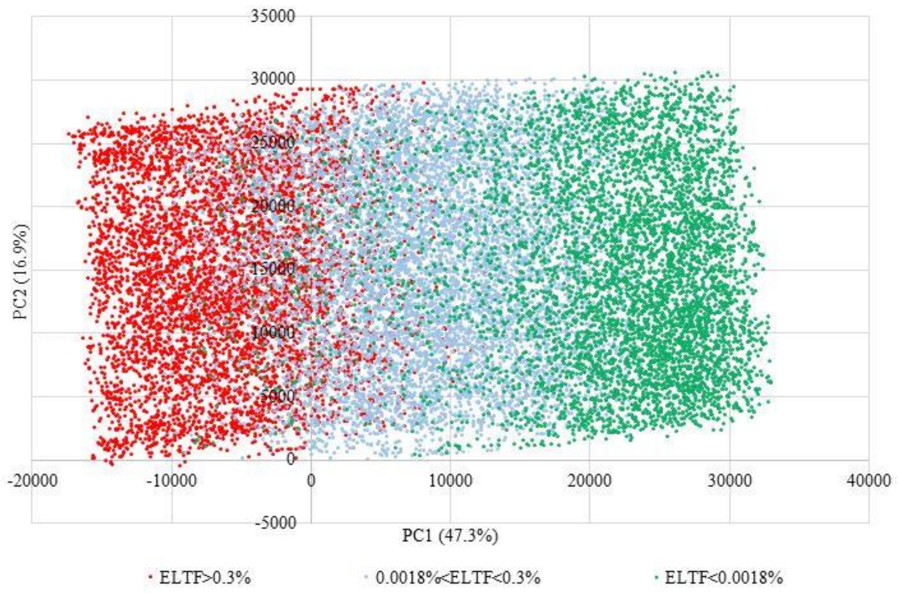
Figure 4 shows the bi-plot for the ELTF clusters, with ELTF value-ranges (represented by different colors) stratifying bands along the y-axis with the colors changing along the x-axis. Pipes with higher values of ELTF (low efficiency) stratify on the left-hand side while pipes with lower values of ELTF stratify on the right side of the bi-plot. This is because ELTF has a high score on PC1, therefore, based on Equation (6) pipes with similar ELTF values (pipei,n) will have similar products of these values and ELTF score on PCn,1 (pipei,n × PCn,1). As Figure 2 indicated ELTF as one of the most influential hydraulic factors (with high score along PC1), the product of pipe parameter values and the ELTF score, based on Equation (6), will then be higher and form bands on the direction shown in Figure 4. Based on Table 4, threshold values of Figure 4 are chosen to distinguish high efficiency pipes in green, low efficiency in red and other values in between in light blue. Further, it is seen that the direction on which the colors of bands change in Figure 4 is the same as the direction of the ELTF vector in Figure 2, i.e., higher values of ELTF, that is tantamount to low efficiency pipes in terms of ELTF, cause these pipes to form a band on the left side of Figure 4 (based on ELTF vector in Figure 2). Similarly, NEE and GEE display clusters of low values (close to zero) on the left hand side and the cluster of higher values (close to 1) on the right hand side. However, because of similar visual result as the ELTF cluster, they are not presented. As general rule, pipes with similar values of metrics expressed with larger vectors (GEE, NEE, ENU and ELTF) tend to cluster more visibly in certain areas of the bi-plots.
Unlike the ELTF, NEE and GEE, ENU stratifications change more closely along the PC2 axis than the PC1 axis, as seen in Figure 5. The direction on which the color of bands changes is the same as the direction of the ENU vector in Figure 2. Values of ENU > 113% that correspond to low efficiency pipes tend to stratify on the bottom (indicated in the color of red) while those that correspond to 100% < ENU < 105% form a horizontal band closer to the top and indicated in green. Other pipes indicated in blue pertain to the other pipes ranging between high efficiency and low efficiency pipes. ENU obtains higher score along PC2, which indicates, first, lower importance compared to GEE, NEE and ELTF (that merit high scores on PC1) and, second, no correlation between the two set of variable. This implies the direction on which the ENU values change has no correlation to that of GEE, NEE and ELTF, as PC1 and PC2 are orthogonal. In other words, efficiency in terms of ENU does not seem to have an effect on efficiency in terms of GEE, NEE and ELTF.
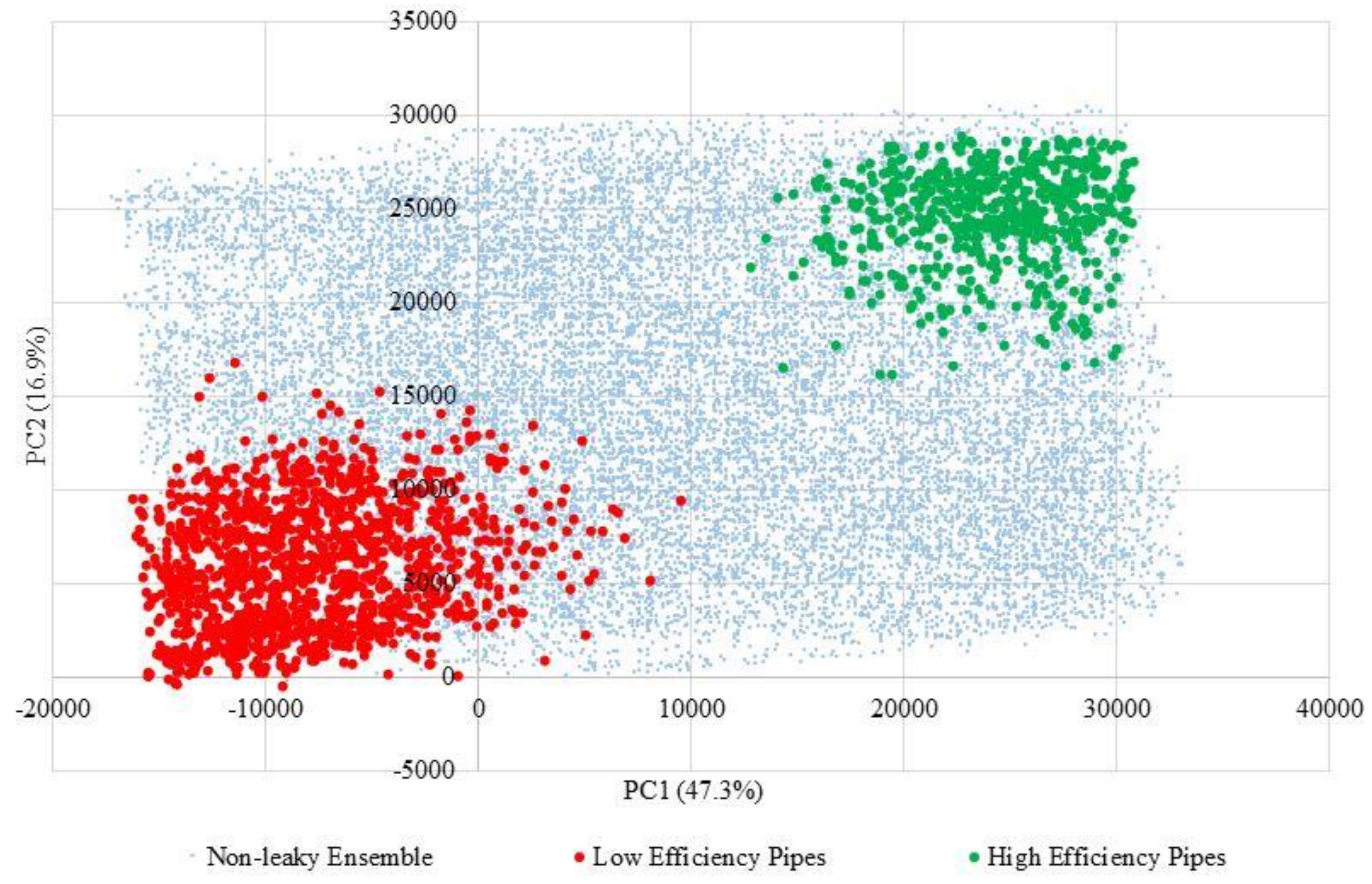
Clusters of high and low efficiency pipes are formed by combining high and low values of energy metrics such as GEE, NEE, ENU and ELTF indicated in Table 4. Therefore, the intersection of vertical bands (from metrics with higher scores on PC1) and horizontal bands (from the metrics with high scores on PC2) forms smaller clusters of high or low efficiency pipes. High-efficiency pipes are defined as summarized in Table 4. However, the purpose of setting thresholds for the metrics is to approximately locate the cluster of high-efficiency pipes on the PCA bi-plots, and not to suggest threshold values for rehabilitation and replacement in practice, as this would be a complex decision task involving multiple factors such as budgetary limitations, risk assessment, water quality, pipe age and break rates, along with energy considerations. The selected thresholds lead to a cluster formed on the top right area of the plot in Figure 6. Similarly, low efficiency pipes cluster are also defined as per summarized in Table 4. The mentioned thresholds create a cluster on the left hand side of the bi-plot. To the extent that stricter values of metrics are desired, the clusters can be smaller or larger, however, the location of clusters will remain the same.
4.2.2. Leaky Ensemble
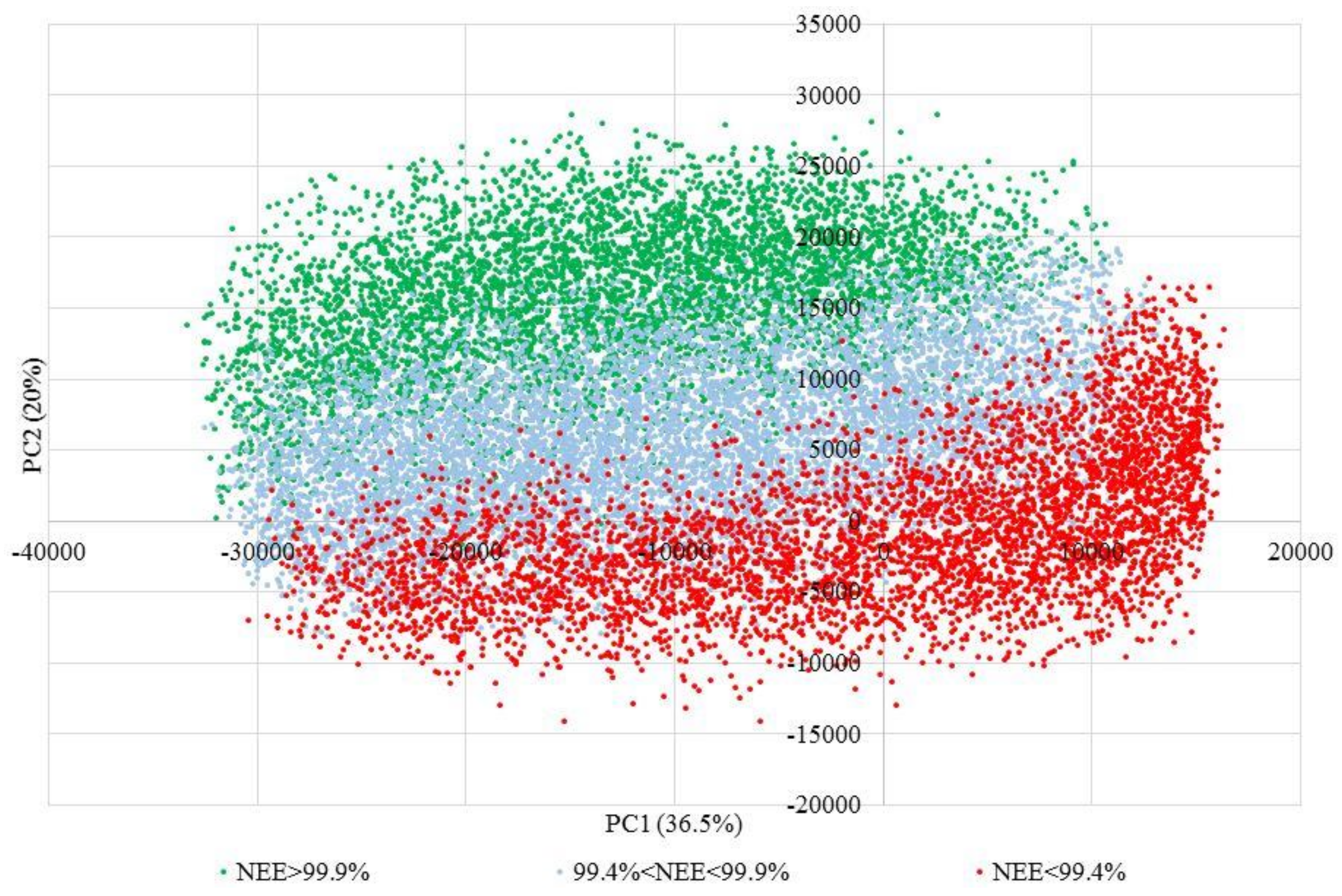
According to Figure 7, pipes with higher NEE values are located in the top left area, while pipes with smaller values of NEE tend to cluster in the bottom right area of the plot. This arrangement of the clusters is mainly because of the direction of NEE axis relative to PC1 and PC2 axes, which makes this set of results different from non-leaky set of pipes. Thresholds of high versus low-efficiency pipes are considered based on Table 4.
From the mono-plot in Figure 3, it was seen that ELTL has a high score on the PC2 axis (value of 0.42) and its corresponding vector is closely aligned with the PC2 axis. This is reflected in the bi-plot in Figure 8, where ELTL values change almost along PC2. High efficiency pipes regarding ELTL (based on Table 4) are clustered at the top (indicated in green), while low-efficiency pipes, on the bottom (indicated in red) and other value ranges (indicated in light blue) are situated in between. Stratifications of metrics values for GEE, NEE and ENU for the leaky ensemble resemble those of the non-leaky ensemble considering the same thresholds, and therefore are not presented here.
The combination of high efficiency values of metrics based on Table 4 results in the cluster of high efficiency pipes on the top left corner of Figure 9, indicated in green. In a similar way, the intersection of low efficiency bands of metrics form the cluster of low efficiency pipes located on the bottom right corner of Figure 9, indicated in red. In addition, similar to the non-leaky ensemble, choosing stricter or more lenient thresholds can result in smaller or larger clusters of high versus low-efficiency pipes; however, the location of the clusters will remain the same. The data points indicated in blue correspond to pipes in the ensemble with an efficiency that is in between the two cohorts of high/low efficiency pipes. Locating high/low efficiency pipes on the bi-plots of Figure 6 and Figure 9 can help identify which hydraulic factors can better point towards these cohorts (considering vectors of hydraulic factors in Figure 2 and Figure 3).
4.3. Examining Current-Practice Pipe Rehabilitations
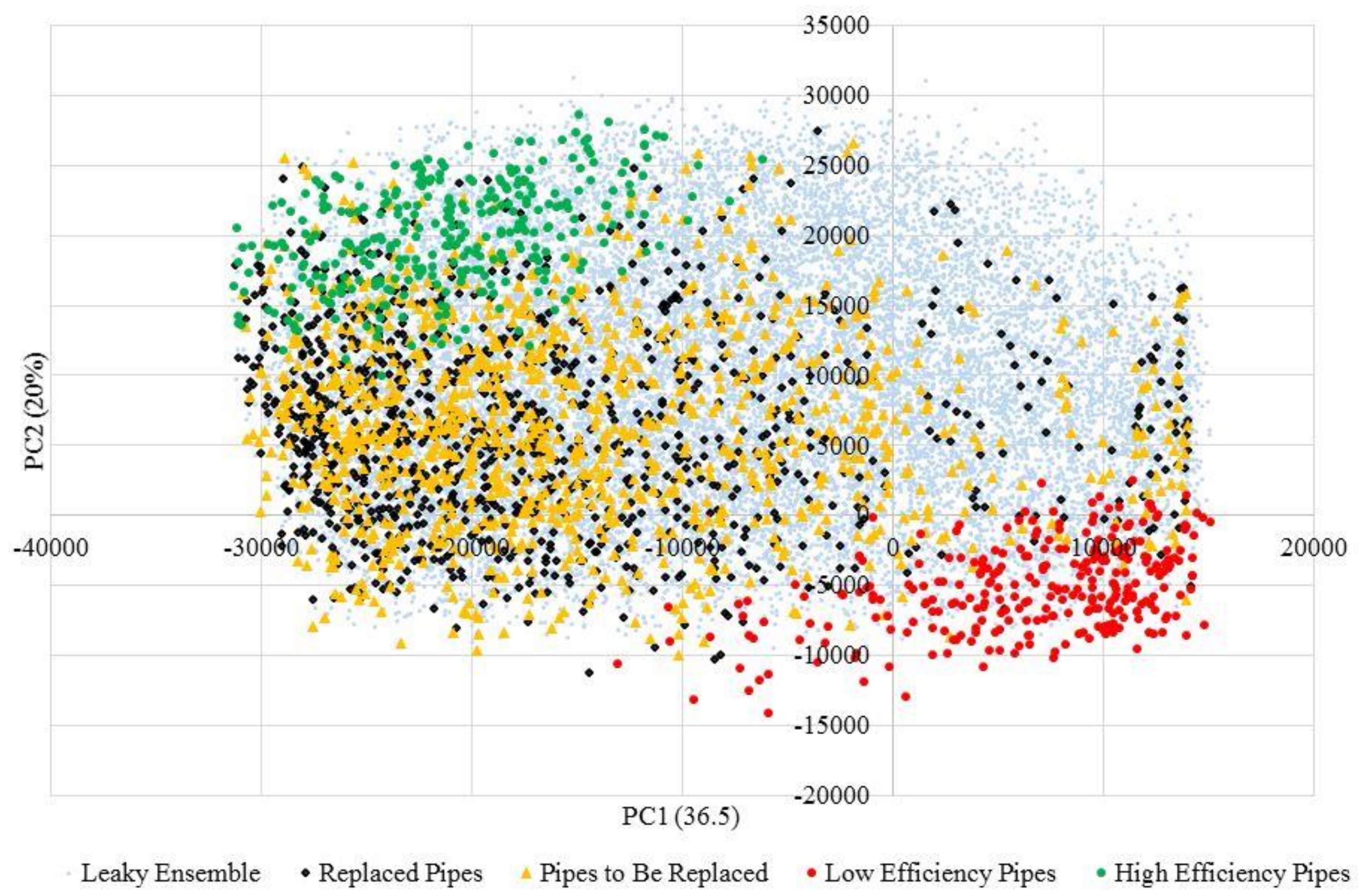
To assess how simplified, common-practice rehabilitation plans would perform from an energy efficiency standpoint, the pipe replacement plan for the leaky ensemble proposed by Prosser et al. [16] was compared to the proposed approach in this paper. The approach proposed by Prosser et al. [16] considers thresholds of 25 breaks per 100 km or 100 years of age in pipes as two alternatives to trigger replacement.
Figure 10 shows the clusters of high and low-efficiency pipes as in Figure 9. In addition, the pipes earmarked for replacement by Prosser et al. [16] beyond the benchmark date (in this case, from 2013 to 2040) are shown as yellow triangles, while previously replaced pipes are shown as black diamonds. It can be seen that many of the pipes to be replaced do not overlap with the low efficiency cluster, as identified through PCA, nor do these pipes move towards high-efficiency pipes after replacement.
5. Discussion
One of the main findings of the analysis was to identify which parameters have the largest influence on describing the variance in energy performance across all pipes in the dataset. Knowing these parameters can help to identify high versus low efficiency pipes.
The PCA results shown through mono-plots in Figure 2 and Figure 3 indicated that of all the hydraulic parameters and energy metrics included in the analysis, NEE, ELTF in both ensembles and ELTL in the leaky ensemble have the highest capacity to describe the variance in the dataset, or, in other words, the energy dynamics landscape, based on their score associated with the two PCs.
Accounting for leakage causes the mono-plot (e.g., Figure 3) and the bi-plots (e.g., Figure 7, Figure 8 and Figure 9) to take a different shape compared to those of the non-leaky ensemble (e.g., Figure 2, Figure 4, Figure 5 and Figure 6). For instance, stratification of similar value ranges for metrics (e.g., ELTF and ENU in Figure 4 and Figure 5) are vertical or horizontal in the non-leaky pipe dataset, while NEE stratifications in the leaky pipes (Figure 7) are diagonal. This result emphasizes the need to consider leakage in energy analysis to fully characterize the complex relationships between friction and flow in individual pipes. Consideration of leakage as shown in Figure 3 causes NEE to take on a distinguished direction compared to other metrics and may potentially identify a different group of low efficiency pipes.
Having categorized high efficiency versus low efficiency pipes, it is of interest to know what characteristics these pipe would have in common, within each cluster. When planning for asset management or rehabilitation, water utilities need to associate highly efficient or low efficiency assets with more familiar decision factors (e.g., pipe size, roughness, unit headloss, pressure, etc.) that would be more readily available, given the level of effort to calculate energy metrics. However, they would also need to know what combination of the readily available decision factors (hydraulic parameters in this study) and with what priority these parameters could be used to better distinguish low from high performance pipes. This objective of the study is achieved by juxtaposition of mono-plots (Figure 2 and Figure 3) and bi-plots (Figure 6 and Figure 9) for each ensemble.
Having located the high and low efficiency categories of pipes on the bi-plot using the criteria in Table 4, comparison of the PCA results for the non-leaky ensemble (Figure 2 and Figure 6) indicates that Ave Q, hydraulic proximity and unit headloss are suitable candidates for identifying the two cohorts of high/low efficiency pipes, based on their vector orientations. It should be noted that, based on the relative importance of these parameters, i.e., the association with the PCs, low efficiency pipes are better characterized by unit headloss (or high Ave Q) compared to pressure. Because of their vector sizes and directions, Elv, D and CHW would not serve as suitable guides to identify high/low efficiency pipes. Although CHW is considered as an influential factor for pipe replacement in practice, the results indicate that this parameter alone is not a suitable representative of energy efficiency.
In a similar way, considering the mono-plot (Figure 3) and the bi-plot (Figure 9) in the leaky ensemble, the best hydraulic parameters with which to identify high/low efficiency pipes are revealed. In this case, the most influential parameters are Ave Q, hydraulic proximity and unit headloss in pipes, because of the size of their corresponding vectors as well as their alignment with the most important principal component, PC1. The next best set of hydraulic parameters includes leakage and pressure, which have relatively less importance in identifying high/low efficiency pipes, because of their alignment with the second most important principal component, PC2. At the same time, the leakage flow itself seems to be more important compared to pressure because of its vector size. Therefore, leakage in pipes, if well characterized, would be a better indicator than pressure for identifying energy efficiency in pipes. Similar to the case for the non-leaky pipe ensemble, Elv, CHW and diameter play a less significant role in characterizing energy dynamics in pipes. In addition, in the leaky ensemble, diameter seemingly has gained more importance due to a longer vector along PC1 in Figure 3. This perhaps corresponds to the correlation of larger pipe sizes and higher flows (not clearly shown in the non-leaky ensemble), due to more accurate model calibration compared to the KY systems, which are the majority of the non-leaky ensemble. However, since diameter does not point directly towards the clusters of high/low efficiency pipes on the bi-plot of Figure 9, they would not be nominated among the most influential parameters in the energy dynamic landscape.
By mathematical definition, Ave Q and hydraulic proximity are more directly reflected in GEE and NEE, in the way that pressure and unit headloss are reflected in ENU and ELTF, and that makes these parameters and their corresponding energy metrics highly correlated. Thus, the hydraulic parameters can be used to target high/low efficiency pipes, as corroborated by mono-plots and bi-plots, particularly given that parameters such as unit headloss and Ave Q are more available to decision makers at water utilities. If leakage is known and well-characterized, it can serve alongside unit headloss and Ave Q as the best candidates for enabling decision makers to effectively earmark high efficiency/low efficiency pipes. In fact, a combination of hydraulic parameters in the form of the resultant vector of unit headloss (or Ave Q) and leakage on the mono-plot of the leaky ensemble has an orientation that would better serve to identify low efficiency pipes. Pipes experiencing high unit headloss (or Ave Q) and high leakage would be the most likely candidates in this case.
To understand how energy dynamics align with replacement programs based upon age of pipe or pipe break rates, Figure 10 placed these methods side by side to high and low efficiency pipes. The results showed that the pipes that would be replaced based upon their age or break rate history are generally not the ones that are the least energy efficient. Although considering energy efficiency alone does not suffice for pipe replacement decision making, the difference in the outcome of the two approaches implies that energy efficiency should be considered in conjunction with other factors such as age, break rate, water quality, payback period and risk assessment to complement the bigger asset management picture, particularly as water utilities seek to become more energy efficient.
6. Conclusions
The goal of the present paper is to explore the patterns and relationships between energy metrics and hydraulic parameters to better understand which parameters have the greatest influence on energy performance of individual pipes. PCA is used to simultaneously visualize the relationships between energy metrics and hydraulic factors and to prioritize these parameters by their importance. This statistical approach helps to reduce the dimensionality of the dataset to allow for identification of combinations of factors that have significant influence on the energy performance of water mains. Two large ensembles comprising over 40,000 pipes juxtaposed the difference in results for systems with and without leakage and highlighted the importance of considering of leakage in large real-world systems when studying their energy dynamics.
The PCA mono-plots show that parameters such as flow, hydraulic proximity of pipes and unit headloss play more important roles in influencing the energy efficiency of pipes compared to leakage and pressure. However, leakage and pressure have a greater impact on the energy efficiency of pipes than diameter, CHW and Elv, which are not well-represented on any of the principal components. However, since leakage and CHW could change throughout the time, it would be a worthwhile study to consider time-based degradation of the leakage and CHW in other efforts.
The PCA bi-plots help to visualize and locate low-versus high-efficiency pipes in a two-dimensional space considering all hydraulic parameters and pipe-level energy metrics. In both leaky and non-leaky cases, clusters of high- and low-efficiency pipes are located on two opposite corners of the plot, and, when considered in conjunction with mono-plots, reveal combinations of hydraulic parameters that would more directly point towards these clusters. The hydraulic parameters of unit headloss and average flow, which are more explicitly involved in mathematical definitions of energy metrics, would serve best in the absence energy metrics.
Overall, energy dynamics along with risk assessment, pipe break rates and age, and water quality, can help to prioritize the replacement and rehabilitation of pipes and should be considered as part of the bigger picture to improve overall water distribution system asset performance. This study has identified several metrics and parameters that could be useful for this purpose moving forward.
Acknowledgments
The authors wish to thank the Natural Science and Engineering Research Council for its financial support of this research. Vanessa Speight received support from the Engineering and Physical Sciences Research Council under grant EP/I029346/1. The authors also thank Hannah Wong from the Department of Civil Engineering, Queen’s University for her helpful comments on editing the text.
Author Contributions
Yves Filion, Vanessa Speight and Saeed Hashemi conceived and designed the experiments; Saeed Hashemi performed the experiments and analyzed the data; Yves Filion and Vanessa Speight contributed reagents/materials/analysis tools; Saeed Hashemi wrote the paper.
Conflicts of Interest
The authors declare no conflict of interest.
References
- Roshani, E.; Filion, Y.R. Event-based approach to optimize the timing of water main rehabilitation with asset management strategies. J. Water Resour. Plan. Manag. 2013, 6, 04014004. [Google Scholar] [CrossRef]
- Rajani, B.; Kleiner, Y. Comprehensive review of structural deterioration of water mains: Physically based models. Urban Water 2001, 3, 151–164. [Google Scholar] [CrossRef]
- Kleiner, Y.; Rajani, B. Comprehensive review of structural deterioration of water mains: Statistical models. Urban Water 2001, 3, 131–150. [Google Scholar] [CrossRef]
- Engelhardt, M.O.; Skipworth, P.J.; Savic, D.A.; Saul, A.J.; Walters, G.A. Rehabilitation strategies for water distribution networks: A literature review with a UK perspective. Urban Water 2000, 2, 153–170. [Google Scholar] [CrossRef]
- Lansey, K.E.; Basnet, C.; Mays, L.W.; Woodburn, J. Optimal maintenance scheduling for water distribution systems. Civ. Eng. Syst. 1992, 3, 211–226. [Google Scholar] [CrossRef]
- Scanlan, M.; Filion, Y.R. Influence of Topography, Peak Demand, and Topology on Energy Use Patterns in four Small to Medium-Sized Systems in Ontario, Canada. Water Resour. Manag. 2017, 4, 1361–1379. [Google Scholar] [CrossRef]
- Pelli, T.; Hitz, H.U. Energy indicators and savings in water supply. J. AWWA 2000, 92, 55. [Google Scholar] [CrossRef]
- Cabrera, E.; Pardo, M.A.; Cobacho, R.; Cabrera, E., Jr. Energy audit of water networks. J. Water Resour. Plan. Manag. 2010, 6, 669–677. [Google Scholar] [CrossRef]
- Cabrera, E.; Gómez, E.; Cabrera, E., Jr.; Soriano, J.; Espert, V. Energy assessment of pressurized water systems. J. Water Resour. Plan. Manag. 2014, 8, 04014095. [Google Scholar] [CrossRef]
- Dziedzic, R.M.; Karney, B.W. Water distribution system performance metrics. Procedia Eng. 2014, 89, 363–369. [Google Scholar] [CrossRef]
- Hashemi, S.; Filion, Y.R.; Speight, V.L. Examining the relationship between unit headloss and energy performance of water mains with statistical analyses across an ensemble of water distribution systems. J. AWWA 2018, in press. [Google Scholar]
- Hashemi, S.; Filion, Y.R.; Speight, V.L. Energy Metrics to Evaluate the Energy Use and Performance of Water Main Assets. J. Water Resour. Plan. Manag. 2017, 2, 04017094. [Google Scholar] [CrossRef]
- Jolliffe, I.T. Principal Component Analysis and Factor Analysis. Principal Component Analysis; Springer: New York, NY, USA, 1986; pp. 115–128. [Google Scholar]
- Krzanowski, W.J. Principles of Multivariate Analysis: A User’s Perspective; Clarendon: Oxford, UK, 1988. [Google Scholar]
- Jolly, M.D.; Lothes, A.D.; Sebastian Bryson, L.; Ormsbee, L. Research database of water distribution system models. J. Water Resour. Plan. Manag. 2013, 4, 410–416. [Google Scholar] [CrossRef]
- Prosser, M.E.; Speight, V.L.; Filion, Y.R. Life-cycle energy analysis of performance-versus age-based pipe replacement schedules. J. AWWA 2013, 105, E721–E732. [Google Scholar] [CrossRef]
- Wong, H.G.; Speight, V.L.; Filion, Y.R. Impact of Urban Development on Energy Use in a Distribution System. J. AWWA 2017, 109, E10–E18. [Google Scholar] [CrossRef]
- Rossman, L.A. Epanet 2 User’s Manual; US Environmental Protection Agency; Water Supply and Water Resources Division, National Risk Management Research Laboratory: Cincinnati, OH, USA, 2000; p. 45268.
- Toolbox, Global Optimization. User’s Guide (r2011b); MathWorks Inc.: Natick, MA, USA, 2011. [Google Scholar]
- City of Toronto. Design Criteria for Sewers and Water Mains; Engineering and Construction Services: Toronto, ON, Canada, 2009. [Google Scholar]
- Region of Peel. Public Works Design. In Specifications and Procedures Manual; Region of Peel: Mississauga, ON, Canada, 2010. [Google Scholar]
- Denver Water. Engineering Standards, 14th ed.; Denver Water: Denver, CO, USA, 2012. [Google Scholar]
- Hashemi, S.; Filion, Y.R.; Speight, V.L. An Energy Evaluation of Common Hydraulic Thresholds in Water Mains. In Proceedings of the 15th International Computing and Control for Water Industry Conference, Sheffield, UK, 5–7 September 2017. [Google Scholar]
- American Water Works Association. AWWA Manual M32-Distribution Network Analysis for Water Utilities; American Water Works Association: Denver, CO, USA, 2017. [Google Scholar]
Figure 1.
Contribution of each PC in the non-leaky ensemble.
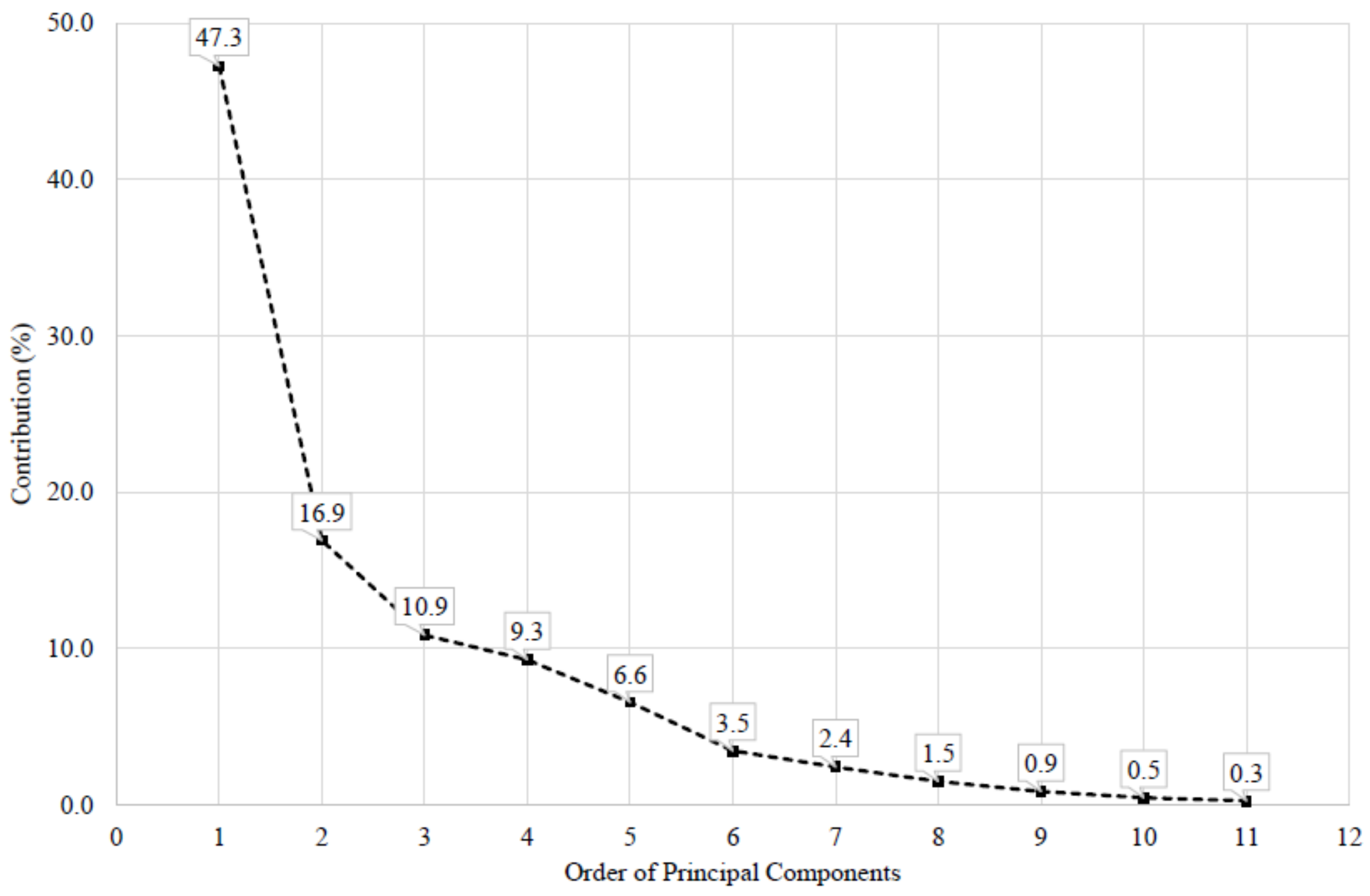
Figure 2.
Mono-plot of variables of interest in the non-leaky ensemble.
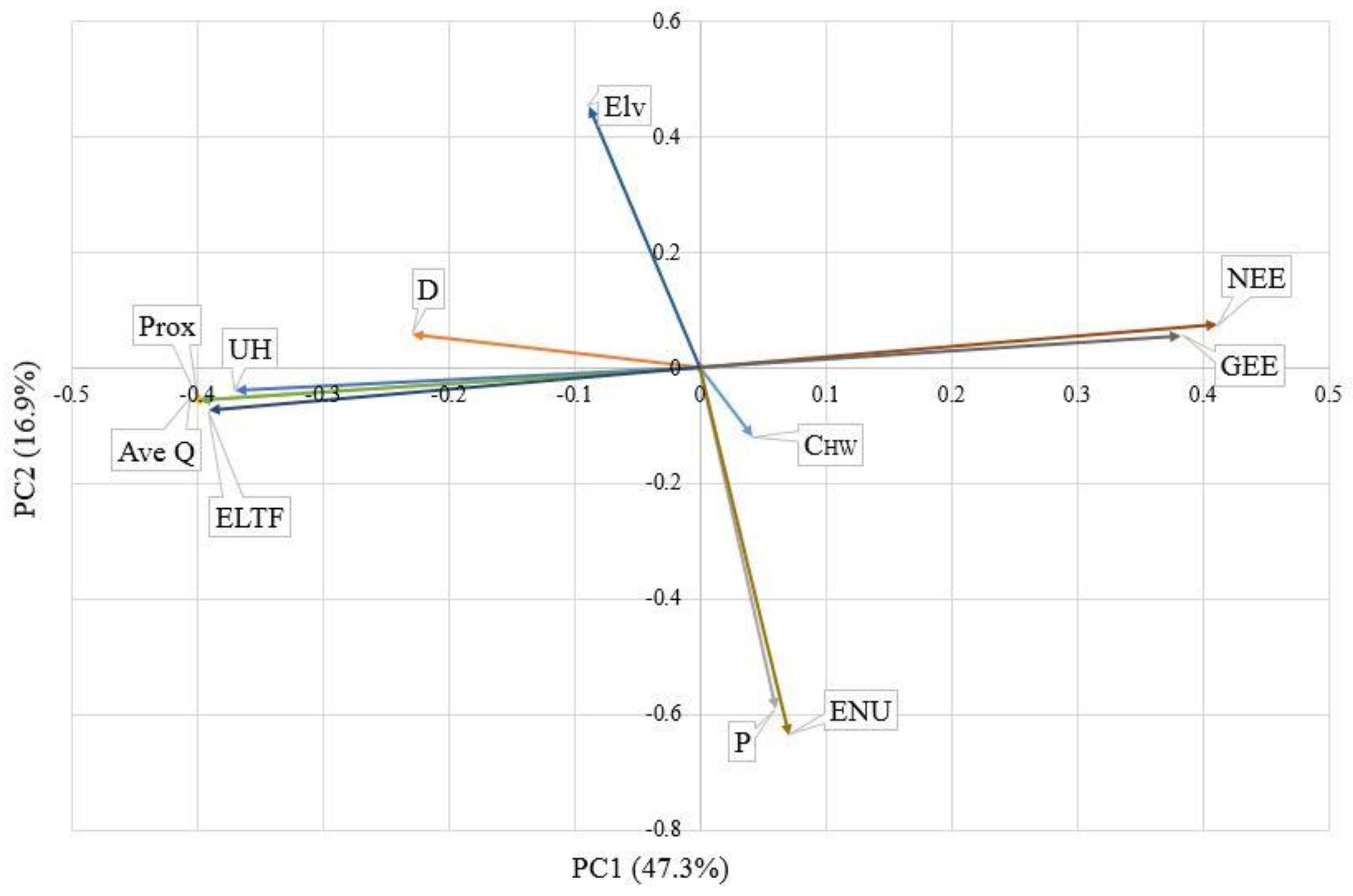
Figure 3.
Mono-plot of all variables of interest in the leaky ensemble.

Figure 4.
Bi-plot of ELTF values in the non-leaky ensemble.

Figure 5.
Bi-plot of ENU values in the non-leaky ensemble.
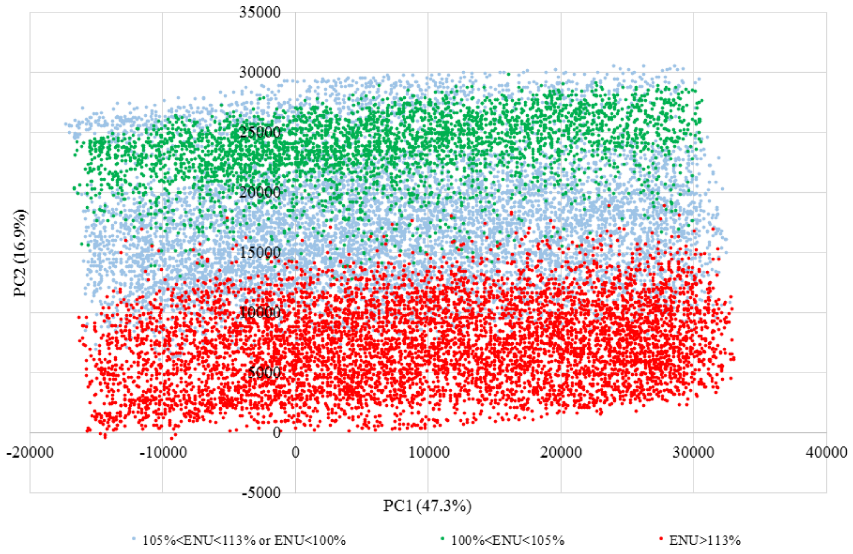
Figure 6.
Bi-plot of high/low efficiency clusters in the non-leaky ensemble.

Figure 7.
Bi-plot of NEE values in the leaky ensemble.

Figure 8.
Bi-plot of ELTL values in the leaky ensemble.
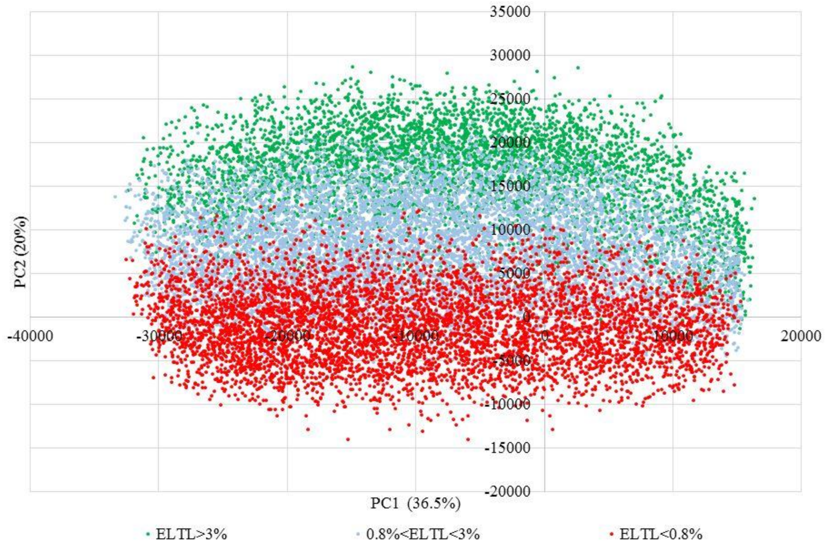
Figure 9.
Bi-plot of high/low efficiency clusters in the leaky ensemble.
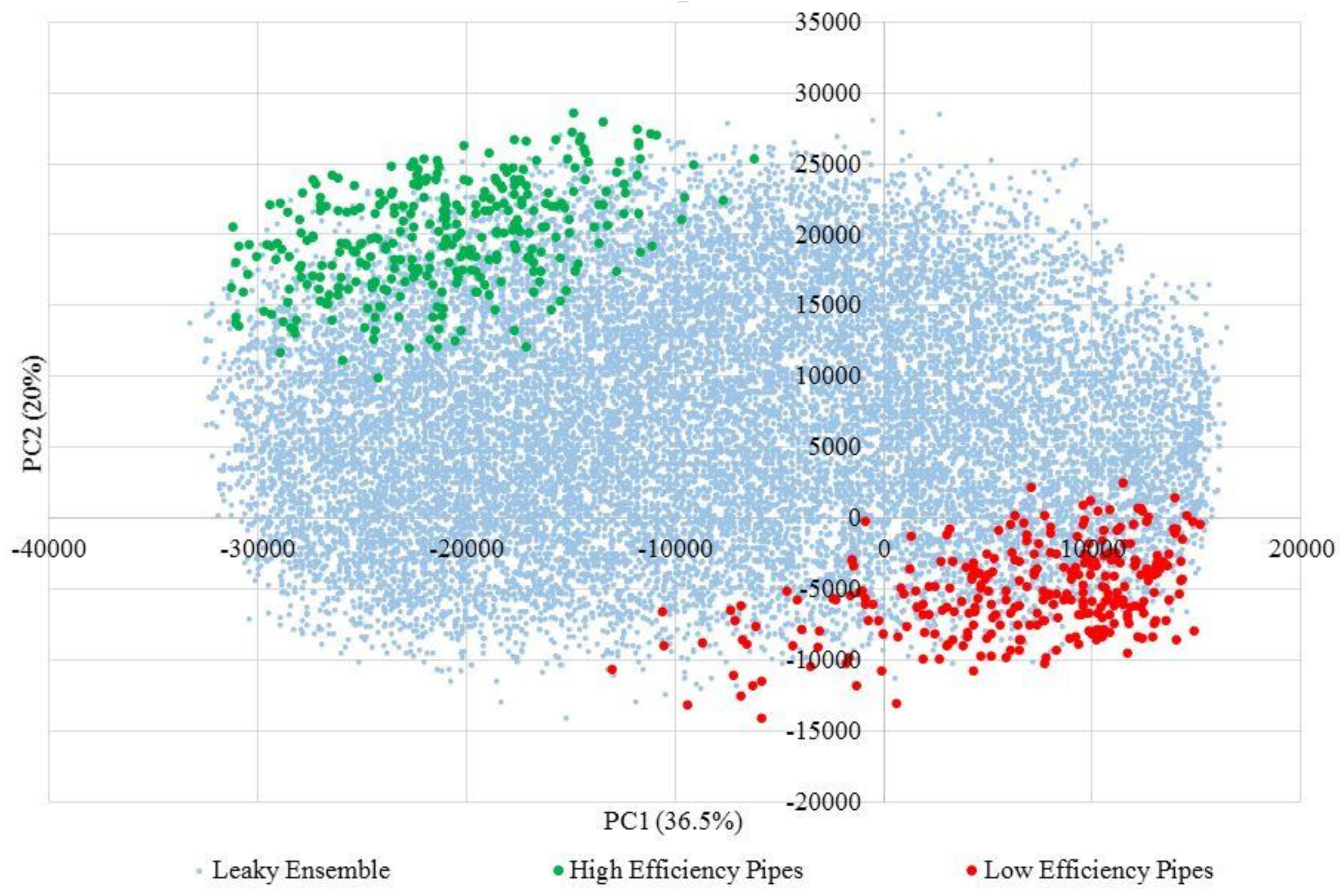
Figure 10.
Bi-plot of high/low efficiency clusters compared to common-practice replacement plan by Prosser et al. [16].
Figure 10.
Bi-plot of high/low efficiency clusters compared to common-practice replacement plan by Prosser et al. [16].


Table 1.
Summary of energy components and metrics by [12].
Table 1.
Summary of energy components and metrics by [12].
| Item | Definition |
|---|---|
| Esupplied | Energy supplied to the upstream end of the pipe |
| Edelivered | Energy delivered to the user to satisfy downstream demand Qd at pressure head Hd |
| Eds | Energy flowing out of the pipe to meet downstream user demands |
| Eleak | Energy directly lost to leakage |
| Efriction | Friction energy loss incurred along the pipe |
| Elocal | Local energy losses through valves, appurtenances, and blockages |
| Eneed | Energy needed/required by the downstream node according to standards |
| Efriction (leak) | Friction energy loss incurred along the pipe as a result of leakage |
| GEE | Gross Energy Efficiency |
| NEE | Net Energy Efficiency |
| ENU | Energy Needed by User |
| ELTF | Energy Lost to Friction |
| ELEL | Energy Lost to Leakage |
| Proximity | Hydraulic proximity to major components of the network based on pressure head and pipe flow |
| Q | Pipe flow (m3/s) |
| Hs | Head supplied at the upstream node of a pipe |
Table 2.
Summary of characteristics of 18 North American WDSs.
| Network | State/Province | No. of Pipes | Pipes Length (km) | No. of Model Junctions | Difference in Elevations (m) a | No. of Pumps | No. of Tanks | Average Daily Demand (MLD) | Average Daily Pressure (m) |
|---|---|---|---|---|---|---|---|---|---|
| 1 | ON1 b | 12,189 | 627 | 11,177 | 50 | 31 | 10 | 69.07 | 44.86 |
| 2 | ON2 | 405 | 56 | 349 | 46 | 6 | 3 | 3.54 | 46.71 |
| 3 | KY1 c | 984 | 67 | 856 | 37 | 1 | 2 | 7.52 | 33.07 |
| 4 | KY2 | 1124 | 152 | 811 | 29 | 1 | 3 | 7.92 | 46.07 |
| 5 | KY3 | 366 | 91 | 271 | 43 | 5 | 3 | 15.19 | 41.76 |
| 6 | KY4 | 1156 | 260 | 959 | 75 | 2 | 4 | 5.65 | 48.02 |
| 7 | KY5 | 496 | 96 | 420 | 75 | 9 | 3 | 8.58 | 134 |
| 8 | KY6 | 644 | 123 | 543 | 96 | 2 | 3 | 6.19 | 60.2 |
| 9 | KY7 | 603 | 137 | 481 | 70 | 1 | 3 | 5.80 | 55.32 |
| 10 | KY8 | 1614 | 247 | 1325 | 135 | 4 | 5 | 9.32 | 54.15 |
| 11 | KY9 | 1270 | 972 | 1242 | 138 | 17 | 15 | 5.07 | 94 |
| 12 | KY10 | 1043 | 435 | 920 | 96 | 13 | 13 | 8.18 | 68 |
| 13 | KY11 | 846 | 464 | 802 | 248 | 21 | 28 | 6.61 | 97.11 |
| 14 | KY12 | 2426 | 655 | 2347 | 145 | 15 | 7 | 5.18 | 111 |
| 15 | KY13 | 940 | 155 | 778 | 95 | 4 | 5 | 8.92 | 50.78 |
| 16 | KY14 | 548 | 105 | 377 | 65 | 5 | 3 | 3.94 | 53.9 |
| 17 | OH1 d | 1183 | 166 | 956 | 100 | 15 | 4 | 10.13 | 57 |
| 18 | OH2 e | 27,231 f | 5500 | 19,618 | 154 | 28 | 27 | 531.49 | 53 |
a: Difference in Elevations = maximum junction elevation (excluding elevated storages) minus minimum junction elevation; b: ON = Ontario; c: KY = Kentucky; d: OH = Ohio; e: OH2 system includes total leakage equivalent to 8% of the total daily demand for nodes; f: Not all the pipes in all systems participate in the statistical analysis.
Table 3.
Correlation matrix of energy metrics and pipe hydraulic factors [11].
Table 3.
Correlation matrix of energy metrics and pipe hydraulic factors [11].
| CHW | D (mm) | P (m) | Avg. Q (L/s) | Avg. Unit Headloss (m/km) | Prox (m4/s) | Elv. (m) | GEE (%) | NEE (%) | ENU (%) | ELTF (%) | |
|---|---|---|---|---|---|---|---|---|---|---|---|
| CHW 1 | 1 | −0.20 | 0.05 | 0.05 | −0.13 | 0.05 | −0.10 | 0.11 | 0.06 | 0.05 | −0.10 |
| D (mm) 2 | −0.20 | 1 | −0.07 | 0.53 | 0.09 | 0.55 | 0.26 | −0.57 | −0.30 | −0.01 | 0.29 |
| P (m) 3 | 0.05 | −0.07 | 1 | −0.02 | −0.08 | −0.05 | −0.24 | 0.10 | 0.08 | 0.66 | −0.10 |
| Avg. Q (MLD) 4 | 0.05 | 0.53 | −0.02 | 1 | 0.73 | 0.96 | 0.16 | −0.75 | −0.81 | −0.13 | 0.73 |
| Avg. Unit Headloss (m/km) 5 | −0.13 | 0.09 | −0.08 | 0.73 | 1 | 0.69 | 0.10 | −0.64 | −0.88 | −0.14 | 0.82 |
| Prox (m4/s) 6 | 0.05 | 0.55 | −0.05 | 0.96 | 0.69 | 1 | 0.18 | −0.73 | −0.78 | −0.08 | 0.71 |
| Elv. (m) 7 | −0.10 | 0.26 | −0.24 | 0.16 | 0.10 | 0.18 | 1 | −0.09 | −0.08 | −0.41 | 0.06 |
| GEE (%) 8 | 0.11 | −0.57 | 0.10 | −0.75 | −0.64 | −0.73 | −0.09 | 1 | 0.80 | 0.04 | −0.76 |
| NEE (%) 9 | 0.06 | −0.30 | 0.08 | −0.81 | −0.88 | −0.78 | −0.08 | 0.80 | 1 | 0.10 | −0.92 |
| ENU (%) 10 | 0.05 | −0.01 | 0.66 | −0.13 | −0.14 | −0.08 | −0.41 | 0.04 | 0.10 | 1 | −0.07 |
| ELTF (%) 11 | −0.10 | 0.29 | −0.10 | 0.73 | 0.82 | 0.71 | 0.06 | −0.76 | −0.92 | −0.07 | 1 |
1: CHW = Hazen–Williams “C” factor; 2: D = Pipe diameter; 3: P = Average daily pressure of a pipe; 4: Avg. Q = Average daily flow of a pipe. However, it is noted that the energy metrics are evaluated based on hourly flows [12]; 5: Avg. Unit Headloss = Average daily unit headloss in a pipe; 6: Prox = Hydraulic proximity of each pipe to major components such as elevated storages and/or pump stations [11,12]; 7: Elv = Arithmetic Average of upstream and downstream nodes of a pipe; 8: GEE = Gross Energy Efficiency (in percent); 9: NEE = Net Energy Efficiency (in percent); 10: ENU = Energy Needed by the User (in percent); 11: ELTF = Energy Lost to Friction (in percent).
Table 4.
Threshold values to define high and low efficiency pipes by [11,23] in both non-leaky and leaky ensembles.
| Energy Metric | Threshold Value to Define Low Efficiency Pipes (%) | Threshold Value to Define High Efficiency Pipes (%) |
|---|---|---|
| GEE | GEE < 15 | GEE > 20 |
| NEE | NEE < 99.4 | NEE > 99.9 |
| ENU | ENU > 113 | 100 < ENU < 105 |
| ELTF | ELTF > 0.3 | ELTF < 0.0018 |
| ELTL * | ELTL > 3 | ELTL < 0.8 |
* ELTL does not apply to the non-leaky ensemble.
© 2018 by the authors. Licensee MDPI, Basel, Switzerland. This article is an open access article distributed under the terms and conditions of the Creative Commons Attribution (CC BY) license (http://creativecommons.org/licenses/by/4.0/).
Share and Cite
MDPI and ACS Style
Hashemi, S.; Filion, Y.; Speight, V. Identification of Factors That Influence Energy Performance in Water Distribution System Mains. Water 2018, 10, 428. https://doi.org/10.3390/w10040428
AMA Style
Hashemi S, Filion Y, Speight V. Identification of Factors That Influence Energy Performance in Water Distribution System Mains. Water. 2018; 10(4):428. https://doi.org/10.3390/w10040428
Chicago/Turabian StyleHashemi, Saeed, Yves Filion, and Vanessa Speight. 2018. "Identification of Factors That Influence Energy Performance in Water Distribution System Mains" Water 10, no. 4: 428. https://doi.org/10.3390/w10040428
Note that from the first issue of 2016, this journal uses article numbers instead of page numbers. See further details here.