On-Bottom Stability Analysis of Cylinders under Tsunami-Like Solitary Waves


Dipartimento di Ingegneria Civile, Università della Calabria, via Bucci, cubo 42B, 87036 Arcavacata di Rende (CS), Italy
*
Author to whom correspondence should be addressed.
Water 2018, 10(4), 487; https://doi.org/10.3390/w10040487
Submission received: 28 March 2018
/
Revised: 11 April 2018
/
Accepted: 12 April 2018
/
Published: 16 April 2018
(This article belongs to the Special Issue Coastal Vulnerability and Mitigation Strategies: From Monitoring to Applied Research
)
Abstract
:A two-dimensional (2D) laboratory investigation on the horizontal and vertical hydrodynamic forces induced by tsunami-like solitary waves on horizontal circular cylinders placed on a rigid sea bed is presented. A series of 30 physical model tests was conducted in the wave channel of the University of Calabria in which a rigid circular cylinder was equipped with 12 pressure transducers placed along its external surface to determine the wave loads, with three wave gauges to record the surface elevation. The observed experimental range was characterized by the prevalence of the inertia component for the horizontal forces and of the lift component for the vertical ones. On the basis of the performance of several time-domain methods, the wave loads and the undisturbed velocity and acceleration derived from the surface elevation of the cylinder section were used to calculate the drag, lift, and horizontal and vertical inertia coefficients in the practical Morison and transverse semi-empirical equations.
1. Introduction
The occurrence of tsunami events in coastal areas is a source of risk for already-vulnerable marine structures subjected to the action of wind waves and currents. Hence, the stability of marine structures under tsunami action depends on the accurate assessment of the hydrodynamic forces. The reproduction of catastrophic tsunami waves like those that occurred in the Indian Ocean in 2004 and in Japan in 2011 was observed to be dependent upon the magnitude of the specific source, and the resulting shapes of surface elevation can be quite different, leading to a generalized modelling of tsunami waves (e.g., [1,2]). Owing to its robust and suitable approach, the modelling of the leading wave of a tsunami event is usually reproduced by the generation of solitary waves both experimentally and numerically (e.g., [3]). Indeed, when tsunami waves approach the coast, the wave trough disappears and only a positive peak remains.
Different studies have been conducted to analyze the propagation of solitary waves and their interaction with structures such as breakwaters or submerged barriers (e.g., [3,4]), although little attention has been paid to the analysis of hydrodynamic forces in the case of horizontal cylindrical bodies. Preliminary studies describe the general features of breaking and non-breaking solitary wave-induced forces on horizontal cylinders ([5,6,7]) but without an extensive approach to study this problem in various wave conditions and positions of the cylinder along the depth. In contrast, for horizontal cylinders under the action of currents or regular and random waves, numerous studies have researched this kind of wave–structure interaction process, adopting different degrees of external roughness of the cylinder and of the sea bed (for a comprehensive review see [8,9]). For bottom-mounted cylinders under the above kind of incident flows, values of hydrodynamic coefficients in Morison-type equations (e.g., [10]) were deduced from field tests [11] as well as small- and large-scale laboratory experiments, and for wide ranges of Keulegan–Carpenter () and Reynolds () numbers [12,13,14,15,16,17,18,19]. More complex models as compared to Morison-type ones and dealing with an improved description of flow-cylinder interaction processes have been also developed [20,21]. More recently, Aristodemo et al. [22] performed a laboratory study on non-breaking solitary wave forces with respect to a horizontal cylinder placed at half-water depth that was supported by numerical simulations based on the smoothed particle hydrodynamics technique (e.g., [23,24,25,26,27,28,29]). In this case, the effect of the free surface was negligible, i.e., there was no scattering, and that related to the bottom was weak. In this context, the horizontal and vertical force regime was dominated by inertia components and the peaks of the horizontal forces were observed to be between about four and five times higher than the vertical ones.
Here, a new laboratory investigation is presented in the case of a bottom-mounted horizontal cylinder subjected to tsunami-like solitary waves. A set of 30 experimental tests was performed in the wave channel of the University of Calabria. A rigid circular cylinder with longitudinal axis parallel to the cross flume was located at the bed of the flume. The horizontal and vertical loads were deduced from the records of 12 pressure sensors arranged along the external surface of the cylinder. Moreover, three wave gauges were placed in correspondence to the vertical axis of the cylinder and close to it to measure the surface elevation, while an ultrasonic sensor located behind the wavemaker was adopted to measure its displacement. The experiments were conducted at intermediate water depths quite close to shallow ones and for ranging from about 0.08 to 0.18, where A is the wave amplitude and d is the water depth, with ranging from about 4 to 7 and 1.83 × < < 3.62 × . The resulting force field was characterized by the prevalence of an inertial regime for the horizontal force and of the lift component for the vertical one. It can be observed that, for of order of , the force regime is completely dominated by the inertia components in both directions (no formation of vortex patters). Moreover, for of order of , there is the prevalence of the drag force component in the horizontal direction and of the lift force in the vertical direction (e.g., [9]). The present experimental values of the free stream kinematics at the transversal axis of the cylinder and of the hydrodynamic forces were adopted to calibrate the hydrodynamic coefficients in the Morison [10] and transverse (e.g., [13]) semi-empirical relationships through the application of ordinary and weighted least square approaches.
The contents of the paper are organized in the following manner. The adopted theory to model tsunami-like solitary waves is summarised in Section 2. The experimental investigation in a laboratory wave channel to determine the horizontal and vertical loads induced by solitary waves on a horizontal cylinder placed on a horizontal bottom is illustrated in Section 3. The adopted semi-empirical formulas for a practical evaluation of the wave forces are explained in Section 4. The characteristics of the incident flow field and the hydrodynamic forces are respectively analysed in Section 5.1 and Section 5.2. The calibration of the semi-empirical equations through the assessment of the hydrodynamic coefficients and their application to assess the contribution of the force components in the present wave–structure interaction phenomenon are respectively described in Section 5.3 and Section 5.4. Finally, conclusions are drawn in Section 6.
2. Tsunami-Like Solitary Waves
Robust and widespread modelling of the leading wave of a tsunami event is given by the solitary wave theory. The time variation of the surface elevation, , is taken as equal to (e.g., [30]):
where is defined as the outskirts decay coefficient and c represents the wave celerity.
The Rayleigh theory to model a solitary wave is here selected due to the stable evolution of this kind of wave along a plane wave flume [31]. Under this approach, and c in Equation (1) are respectively determined as:
where = 2k and k is the wave number which is considered a finite quantity for engineering purposes even if the wave length, L, of a solitary wave is theoretically taken as equal to infinity. As a result, an apparent wave period is defined as T = L/c and an apparent wave length L = 2/k is then used. The above quantity is determined assuming, at a distance of L/2 away from the wave crest, the value of is reduced to 1% of its maximum value (e.g., [22,32]). Other heuristic methods to define a finite wave length lead to negligible differences in defining a finite time window to analyse the present physical process (e.g., [33]).
Following the Rayleigh theory, the horizontal (u) and vertical (v) velocity values induced by the passage of a solitary wave are calculated as (e.g., [34]):
where z is the vertical coordinate starting from the bed and , , , , , and are equal to:
The analytical expressions to calculate the horizontal ( = /) and vertical ( = ) accelerations read as:
The second-order solution given by Equation (3) leads to a small variation of u and v along z. This is in agreement with the intermediate water depth conditions close to shallow ones as observed through the present laboratory experiments. The free stream velocity field, in conjunction with the acceleration one, will be used in the practical Morison and transverse equations in order to calculate the hydrodynamic coefficients.
A non-linear solution of the horizontal movement for a piston-type paddle, X, able to generate a solitary wave based on the Rayleigh solution is used [31]:
3. Experimental Tests
Two-dimensional experimental tests were conducted in the wave flume at the GMI Laboratory of the University of Calabria. The wave channel is 41.0 m long, 1.2 m deep, and 1.0 m wide, with the sidewalls and bottom made of glass. It is equipped with a piston-type wavemaker with a maximum stroke S = 0.5 m, and a rubble mound breakwater (slope of 1:4) to dissipate the incoming waves. More specifically, the paddle movement is controlled indirectly by the rotation of a joint of the mechanical chain, which is connected to the paddle. The rotation angle is measured with a resistive encoder that provides a proportional analogue voltage signal. This signal, as well as the set-point signal, is processed by a properly tuned proportional integral derivative (PID) controller. The PID acts in order to minimize the error, i.e., the difference between the set-point and the feedback signals. The output of the PID is connected to the kinematic chain through a hydro-pneumatic actuator. The set-point signal is generated by a Data AcQuision Board (DAQ), thanks to a digital-to-analog converter (DAC) (see, for more details, Tripepi et al. [35]). The longitudinal profile of the experimental layout is highlighted in Figure 1.
At about 9 m from the wave paddle, a circular cylinder with diameter D = 0.127 m was placed at the bottom flume ( = 0, where e is the distance between the bottom of the cylinder and the bed) with its longitudinal axis orthogonal to the wave direction (Figure 2a). This physical model was installed in the channel by means of a steel support equipped by a pulley system in order to accurately choose a specific location along the depth. To ensure unwanted displacements of the cylinder, C-shaped PVC supports were used at its edges (see Figure 2b). Moreover, a special glue was adopted to fix the cylinder at the bottom in order to inhibit the passage of water flows below it. Twelve pressure transducers (PDCR1830 model by Druck) were acquired in differential mode due to the Wheatstone-bridge configuration and mounted along the external surface of the cylinder at 30 intervals. Similar to the experimental tests with wind waves and currents performed by Aristodemo et al. [19,20], the transducers were slightly staggered along the longitudinal axis of the central part of the cylinder to avoid the use of a too-large diameter (see Figure 2a). The obtained dynamic pressures, , were determined by subtracting the static pressures from the records of total pressures measured by the transducers. The values of were assumed constant over the influence areas and evaluated as a function of the position of the transducers. Then, the horizontal () and vertical (,) hydrodynamic forces were deduced as:
where the influence areas , and are evaluated as:
The reference angle, , was considered starting from the lower side of the cylinder in clockwise direction (Figure 2c).
A resistive wave gauge by Edif Instruments was located in correspondence to the vertical axis of the cylinder to measure the surface elevation and successively deduce the undisturbed kinematic field at the transversal axis of the cylinder for the application of semi-empirical equations. A further two wave gauges were placed 1.1 m before and after the vertical axis of the considered structure in order to check the value of c obtained by Equation (2) on the basis of the time shifts observed during the propagation of the solitary waves. The wave gauges were acquired in single-ended mode. The sampling frequency (f) of the transducers and gauges was set at 1000 Hz. Both types of instruments were calibrated in static conditions using a water tank equipped with a digital water gauge and a bottom spillway. Measurements were performed every 0.02 m and, for each water level, the signals were acquired for 10 min. All instruments provided a linear calibration function. To verify the correct generation of the solitary wave by applying Equation (6), the horizontal displacement of the piston, X, was measured by an ultrasonic sensor located behind the position at rest of the paddle using f = 50 Hz (see Figure 1).
A set of 30 different experimental tests at increasing A was performed by changing the motion law in the possible range of the stroke S of the present piston-type paddle. Each wave amplitude was generated two times in order to check for repeatability of the experiments. The still water depth, d, of the experimental tests was 0.4 m. Table 1 shows the resulting values of A, T, , = , = and (relative depth), where is the maximum value of the free stream horizontal velocity at the transversal axis of the cylinder, and is the kinematic viscosity.
It is worth noting that the experimental values of T sometimes highlight a deviation from a decreasing theoretical trend when A increases. This is due to the significant spreading of around the undisturbed free surface because of the occurrence of the so-called trailing waves [31]. However, the maximum amplitudes of trailing waves are up to 2% of those related to the solitary waves, leading to a slight influence on the final part of the wave loads for which the magnitude is usually low and then irrelevant for stability purposes. The values of the experimental trailing waves were observed to be under the critical threshold suggested by Guizien and Barthélemy [31]. The above features also influence the values of and, similarly to the definition of an apparent wave period, it is possible to define an apparent Keulegan–Carpenter number [22]. This parameter was generally linked to the occurrence of vortices around the cylinder and, more generally, used to study the wave-cylinder interaction processes (e.g., [8]). The values of will be successively adopted for comparisons with regular wave cases in the literature. It can also be noted that the range of refers to intermediate water depths quite close to shallow ones, allowing for the use of Equation (3) to represent the undisturbed kinematic field at the cylinder location.
4. Semi-Empirical Formulas
For engineering purposes, the use of semi-empirical formulas represents a simple and suitable tool to determine the horizontal and vertical hydrodynamic loads acting on offshore and coastal structures. Owing to their mathematical representation, these formulas require a specific calibration of the hydrodynamic coefficients for their correct application. In the case of in-line loads, the Morison equation [10] is widely adopted for various incident flows and kinds of structures, while the transverse equation (e.g., [13,35]) is adopted to model the vertical forces. It is worth noting that the use of Morison and transverse formulas is here possible since no diffraction effects occur, i.e., the presence of the physical model of the bottom-mounted cylinder does not affect the local free surface, which is considered as a rigid lid [6].
In this context, the in-line force, , is evaluated as the sum of a drag component, , due to the resistance of a solid body to the incident flow motion, and an inertia component, , depending on the horizontal acceleration of the oscillatory flow. The total horizontal force, , is calculated as follows [10]:
where represents the drag coefficient and is the horizontal inertia coefficient. The values of u and are the ambient horizontal velocity and acceleration at the transversal axis of the cylinder, respectively.
The total vertical load, , is given as the superimposition of a lift component, , generated by the increased flow velocity across the cylinder induced by the blocking of the flow, and an inertia component, , depending on the vertical acceleration of the external flow at the transversal axis of the body. The transverse force is then written as [13]:
where is the lift coefficient and is the vertical inertia coefficient. The value of is the free stream vertical acceleration. It can be observed that, for = 0, the contribution of is usually considered negligible (e.g., [14,20]) even if this force contribution affects the magnitude and the shape of the total vertical force and it is here considered as in the case with = 1 [22]. Indeed, for > 0, the value of becomes relevant in modelling , as highlighted by Aristodemo et al. [22].
The undisturbed kinematic field, i.e., u, , and , in the Morison and transverse schemes was determined by Equation (3) from the experimental values of the surface elevation, , deduced from the wave gauge placed at the vertical section of the cylinder.
5. Results
5.1. Surface Elevation and Kinematic Field
The evaluation of the solitary wave loads at the horizontal cylinder placed on the bottom channel depends on the suitable values of surface elevation at the cylinder section and the related free stream kinematic field at the cylinder, in addition to the correct generation of the solitary wave by the experimental piston paddle. Figure 3 highlights the comparison between the analytical solution given by Equation (1) and the experimental values of the surface elevation at the vertical axis of the cylinder for test number 5 (A = 0.037 m and T = 3.91 s, i.e., solitary wave with low amplitude and broad shape) and test number 30 (A = 0.071 m and T = 2.86 s, i.e., solitary wave with high amplitude and narrow shape), respectively. For both cases, a general good agreement on the incident solitary waves can be noticed, particularly for the higher values of . The reference time instant t = 0 refers to the passage of the solitary wave crest at the vertical section of the cylinder.
With reference to test number 30, Figure 4 shows the comparison between analytical solutions and laboratory tests for the time variation of the ambient kinematic field in correspondence with the transversal axis of the cylinder, namely z = D/2, where the semi-empirical schemes will be applied. Starting from the surface elevations (see Figure 3b), u was directly determined by applying Equation (3), while and were respectively derived from u and v (see Equation (5)). Specifically, Figure 4a describes the time history of the horizontal velocity u where it is possible to notice the same shape of (see Figure 3b). The theoretical horizontal acceleration, , shows equal positive and negative peaks (Figure 4b), while the analytical vertical acceleration, , presents a double positive peak and a greater negative one (Figure 4c). Small experimental deviations from the reference analytical solutions occur in the final part of the passage of the solitary wave across the cylinder, leading to slight non-symmetrical features of the values of u, , and . However, these discrepancies are essentially not relevant for stability purposes of the cylinder in which the force peaks play a fundamental role. As later highlighted, the relevance of the ambient kinematic field at the cylinder arises from the influence on the shape of the horizontal and vertical hydrodynamic loads as well as in the application of Morison and transverse semi-empirical schemes in which the various force components are directly proportional to u, , and .
5.2. Hydrodynamic Forces
In this section, the time history of the solitary wave loads acting on the bottom-mounted cylinder deduced from the experimental tests are analyzed. As previously shown in Figure 3 for the surface elevation, two reference test cases characterized by a different wave amplitude and period are considered.
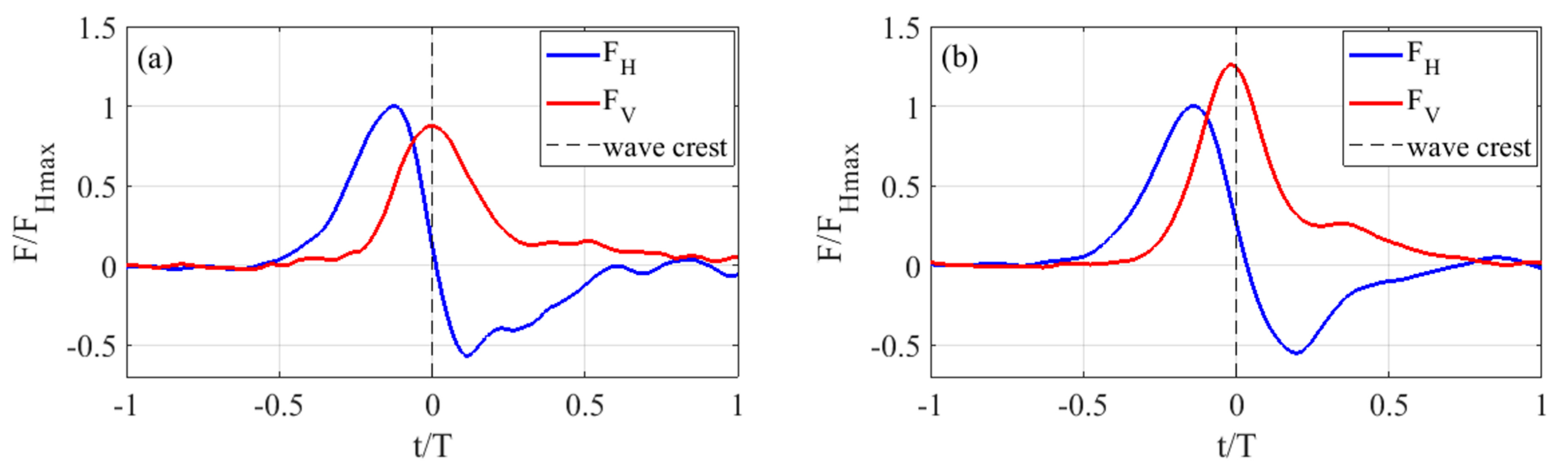
Figure 5a,b highlight the experimental values of the horizontal () and vertical () hydrodynamic forces induced by solitary waves for test numbers 5 and 30, respectively. The black dashed vertical line refers to the occurrence of the wave crest at the vertical section of the cylinder, i.e., the time instant t = 0 in which the maximum surface elevation and horizontal velocity appear. It is interesting to observe that, in terms of maximum peaks, is greater than for test number 5 (lower solitary wave), while > for test number 30 (higher solitary wave). Moreover, a prevalence of positive values of the forces can be noticed, revealing that the cylinder is substantially subjected to the coupled action of a forward motion in the direction of solitary wave propagation and a lifting one towards the free surface. For test number 5, the maximum peak of is more back-shifted than the other case if compared to the passage of the solitary wave crest. In both cases, there is a prevalence of the inertia component with respect to the contribution of the resistance offered by the presence of the cylindrical structure. The above findings are substantially in agreement with experimental observations related to the interaction between regular or random waves and cylinders placed on the bed when the parameter is considered (e.g., [15,36]). It can be observed that the shapes of generally follow those related to , with a less relevant contribution of the drag force related to the decreasing of the negative peak of and the forward shift of the positive peak of . Apart from a small contribution of the vertical inertia component for low values of , the shape of the vertical load, for reference test numbers 5 and 30, follows that related to the horizontal velocity where the peak appears very close to the solitary wave crest. This situation arises when an external flow interacts with a bottom-mounted cylinder in which the lift component dominates the features of (e.g., [14,19]). The occurrence of drag and lift forces will be better highlighted when Morison and transverse semi-empirical schemes are applied. However, it is important to notice that these contribution are linked to the formation of vortex patterns around the cylinder and the consequent deviation from a pure inertial field instead characterized by a potential flow (e.g., [37,38]).
Taking into account all experimental tests, the positive and negative maximum horizontal forces ( and ) and the positive maximum vertical forces () as a function of are respectively shown in Figure 6. Note that these peaks are respectively normalized with respect to the positive maximum peak of the vertical force, *. As commonly carried out in the field of solitary waves interacting with offshore and coastal structures (e.g., [39]), the non-dimensional wave amplitude, , will be considered as simple representative parameter to evaluate the features of the hydrodynamic forces and coefficients compared to and since these parameters are dependent on the indirect knowledge of the undisturbed horizontal velocity at the transversal axis of the cylinder. Moreover, a more stable trend of the involved quantities when is adopted was observed. In general, the positive peaks increase almost linearly with , while the negative ones highlight a higher variation for > 0.15. The values of are lower than the positive ones and those referring to . It is interesting to note that, for < 0.105, values are slightly greater than , while values are greater than values for > 0.105 and, particularly, for high . The threshold corresponding to = 0.105 is highlighted in Figure 6 with a grey dashed vertical line. Considering the whole experimental range of , the values of and respectively exhibit an increase of 57% and 56%, with growth of about 69%.
5.3. Calibration of Semi-Empirical Formulas
The calibration of Morison and transverse semi-empirical formulas to evaluate the solitary wave forces at bottom-mounted cylinders in an easy way is linked to the correct evaluation of the hydrodynamic coefficients. The above time-constant coefficients can be viewed as representative parameters of the complex flow field around the cylinder. In order to minimize the differences between experimental forces and those calculated by Morison and transverse schemes within the adopted apparent wave period, time-domain methods for evaluating the hydrodynamic coefficients were considered. The knowledge of the ambient kinematics field (i.e., horizontal velocity and horizontal and vertical acceleration) at the transversal axis of the cylinder and the hydrodynamic loads acting on it deduced through the experimental tests allowed for the calculation of in-line ( and ) and transverse ( and ) hydrodynamic coefficients. In this context, the ordinary and weighted least square methods were used (e.g., [40]). In the weighted least square method, the difference between the measured and the semi-empirical force is multiplied by , with k a positive index. Within the adopted apparent wave period of the solitary wave at the cylinder, the hydrodynamic coefficients and related to the Morison scheme are calculated as:
where and . The value of M represents the number of force and kinematic values within the adopted wave period.
Similarly, the expressions to determine the hydrodynamic coefficients and for the transverse formula read as:
where = and = . Equations (11) and 12 recover the ordinary least square approach by setting k = 0.
The performances of the ordinary and weighted least square approaches for calculating , , , and are analysed on the basis of the mean square error percent (MSEP). The MSEP was obtained by comparing Morison and transverse forces and those calculated experimentally in the following way:
where represents the generic semi-empirical force and is the generic experimental one.
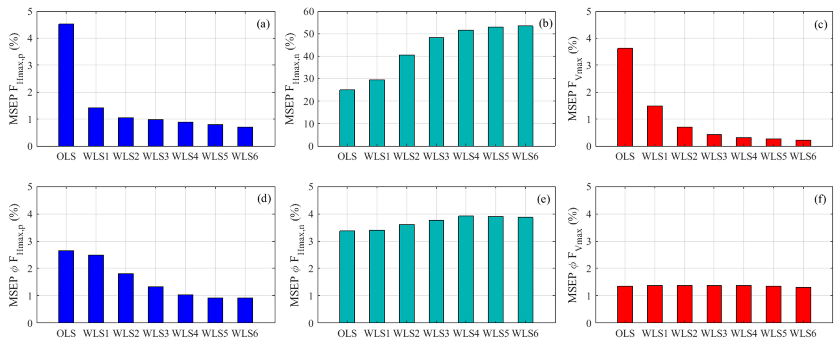
For practical aims, attention was paid to the maximum peaks of the wave forces, i.e., positive and negative for the horizontal force and only positive for the vertical one, and the related phase shifts, , where is the occurrence time of the maximum positive or negative peak within the wave period. Figure 7 describes the mean values of MSEP for all 30 laboratory tests calculated by the ordinary least square (OLS), the weighted least square using k = 1 (WLS1), k = 2 (WLS2), k = 3 (WLS3), k = 4 (WLS4), k = 5 (WLS5), and k = 6 (WLS6). The choice to test the weighted least square method up to k = 6 is to capture the maximum positive peaks of the horizontal and vertical hydrodynamic loads without any overestimation of the above quantities. The values of MSEP linked to the positive peaks of both forces are lower than those related to the negative horizontal forces. When k increases, MSEP for tends to decrease, ranging from about 4.5% for k = 0 to 0.7% for k = 6. The same feature refers to for which the MSEP ranges from about 3.6% for k = 0 to 0.2% for k = 6. Conversely, MSEP strongly increases proportionally to , moving from 24% for k = 0 up to 54% for k = 6. With regard to the phase shift associated with the force peaks, the resulting values of MSEP prove to be generally low and oscillate between 0.9% and 4.9%, with lowest values for associated with k = 6 and lowest values for using k = 0. Taking into account the mean values of MSEP related to all force peaks and associated phase shifts, it is possible to observe that the OLS method (k = 0) gives the lowest MSEP, equal to 6.7%. Although the use of k > 1 leads to good values of the maximum peaks of both forces, a relevant overestimation of the negative peak of is noted. Then, the ordinary least square method was considered to determine the hydrodynamic coefficients in the Morison and transverse equations.
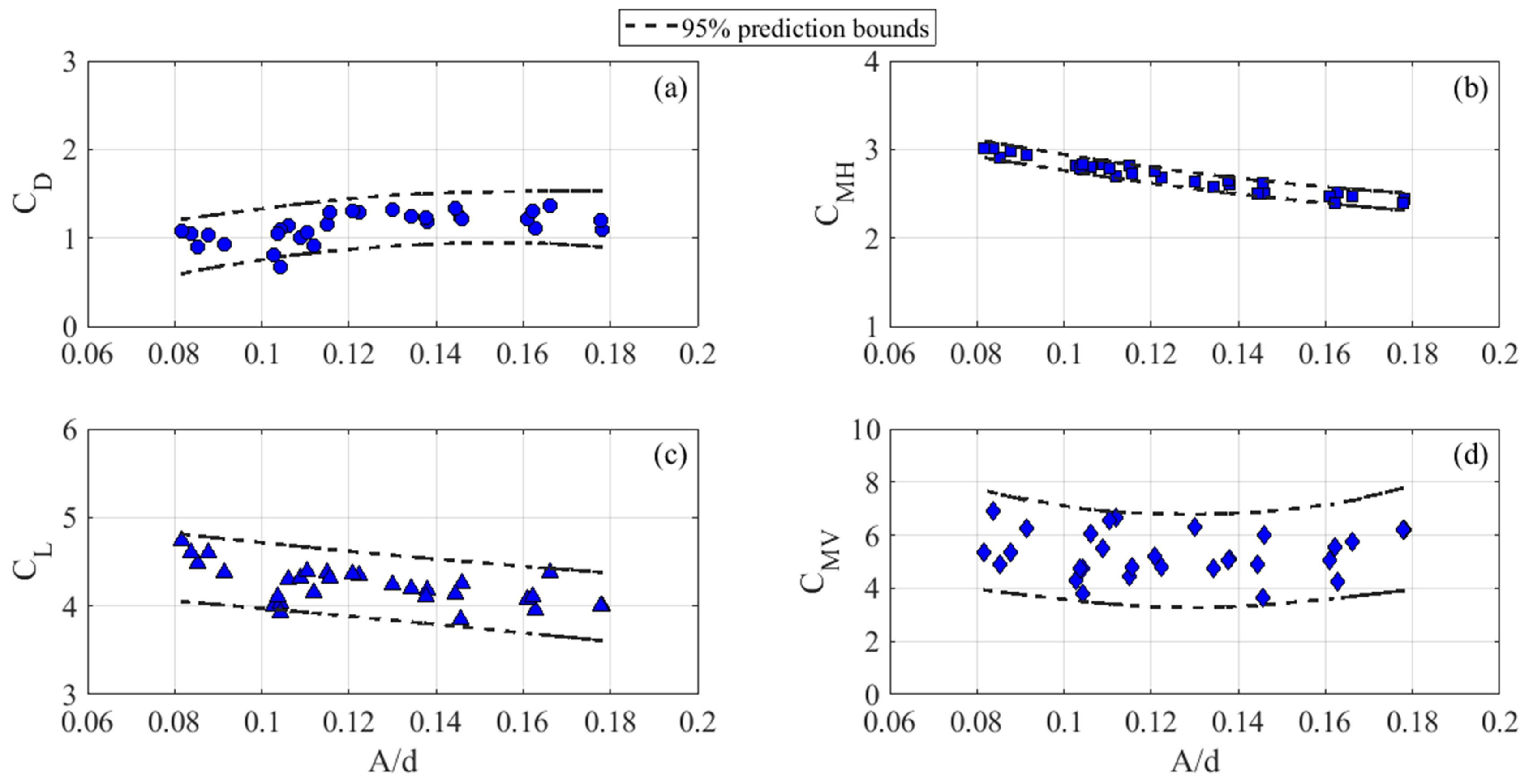
Figure 8 highlights the experimental values of , , , and in the Morison and transverse semi-empirical equations as a function of ranging from 0.08 to 0.18. The 95% prediction intervals are also plotted in Figure 8 and based on second-order polynomial fitting curves for , , and and on an exponential fitting equation for . Similar to the case with = 1 [22], the hydrodynamic coefficients , and show a general decreasing trend when increases. This feature is particularly evident for the stable trend of horizontal inertia coefficient, while for the corresponding vertical one the trend is quite scattered, i.e., with the highest uncertainty, even if this kind of force component has a small weight in calculating the vertical load as compared to the lifting load, as successively highlighted in the application of semi-empirical force models. The values of generally tend to increase up to approximately = 0.15 with a corresponding = 1.4, followed by a tendential reduction. This particular feature can be heuristically explained through the formation of vortex patterns around the cylinder that allows the occurrence of drag and lift force components at the cylinder. Indeed, for low and , the increasing trend of is linked to a predominant transverse direction of the vortices compared to the incoming flow direction, while the decreasing trend of is related to a resulting movement of the vortices in the direction of the incident flow, as observed experimentally for regular waves by Sumer et al. [41] and numerically for solitary waves by Aristodemo et al. [22]. Regarding the magnitude of the hydrodynamic coefficients, values range from 0.7 to 1.4, from 2.4 to 3, from 3.9 to 4.7, and from 3.7 to 6.9.
In a slightly wider experimental range (4 < < 8), the hydrodynamic force coefficients , , and are also plotted vs. in Figure 9 and compared with literature experimental results referring to regular waves interacting with a bottom-mounted cylinder. Only the vertical inertia coefficients were not reported since no experiments were conducted in the present range. To the author’s knowledge, the unique experiments by Cheong et al. [13] to determine were performed out of the investigated range, i.e., 0.05 < < 1.25, even if a decreasing trend when increases was noted as in the present dataset. A more scattered range for compared to can be observed since the Keulegan–Carpenter number depends on the apparent wave period which suffers from small oscillations near the free surface due to the appearance of spurious trailing waves. Figure 9a shows the present values of as a function of plotted against the experiments conducted by Sarpkaya and Rajabi [12], and Bryndum et al. [14] through a non-linear fit of the laboratory data (Neill and Hinwood [15] and Chevalier et al. [16]). Comparing the values of , the authors observed an overall good agreement with the non-linear fit carried out by Bryndum et al. [14] and a slight underestimation of the present experiments as compared to those performed by Sarpkaya and Rajabi [12], Neill and Hinwood [15], and Chevalier et al. [16], even if few values of are present in the above works. With regard to , Figure 9b shows the comparison between the current dataset and the values obtained by Sarpkaya and Rajabi [12], Bryndum et al. [14], Neill and Hinwood [15], Chevalier et al. [16], and Aristodemo et al. [19]. The present values of are lower than those calculated by Sarpkaya and Rajabi [12], Bryndum et al. [14] and, in particular, by Aristodemo et al. [19], while they are slightly higher than those obtained by Neill and Hinwood [15] and Chevalier et al. [16]. However, the current values of tend to an asymptotic value equal to 3.29 occurring for the potential flow characterized by only inertia forces (very low numbers) deduced from the studies of Bryndum et al. [14] and Sumer and Fredsoe [9]. Paying attention to (see Figure 9c), the present data are compared with those obtained by Sarpkaya and Rajabi [12], Bryndum et al. [14], Neill and Hinwood [15], and Aristodemo et al. [19]. The agreement with the fitting curve proposed by Bryndum et al. [14] is very good, while the current values of underestimate those proposed by Sarpkaya and Rajabi [12] and strongly overestimate those obtained by Neill and Hinwood [15] and Aristodemo et al. [19]. As for , it can be noted that tends to an asymptotic value equal to 4.49 for the fully inertial regime, i.e., when →0.
5.4. Use of Semi-Empirical Formulas
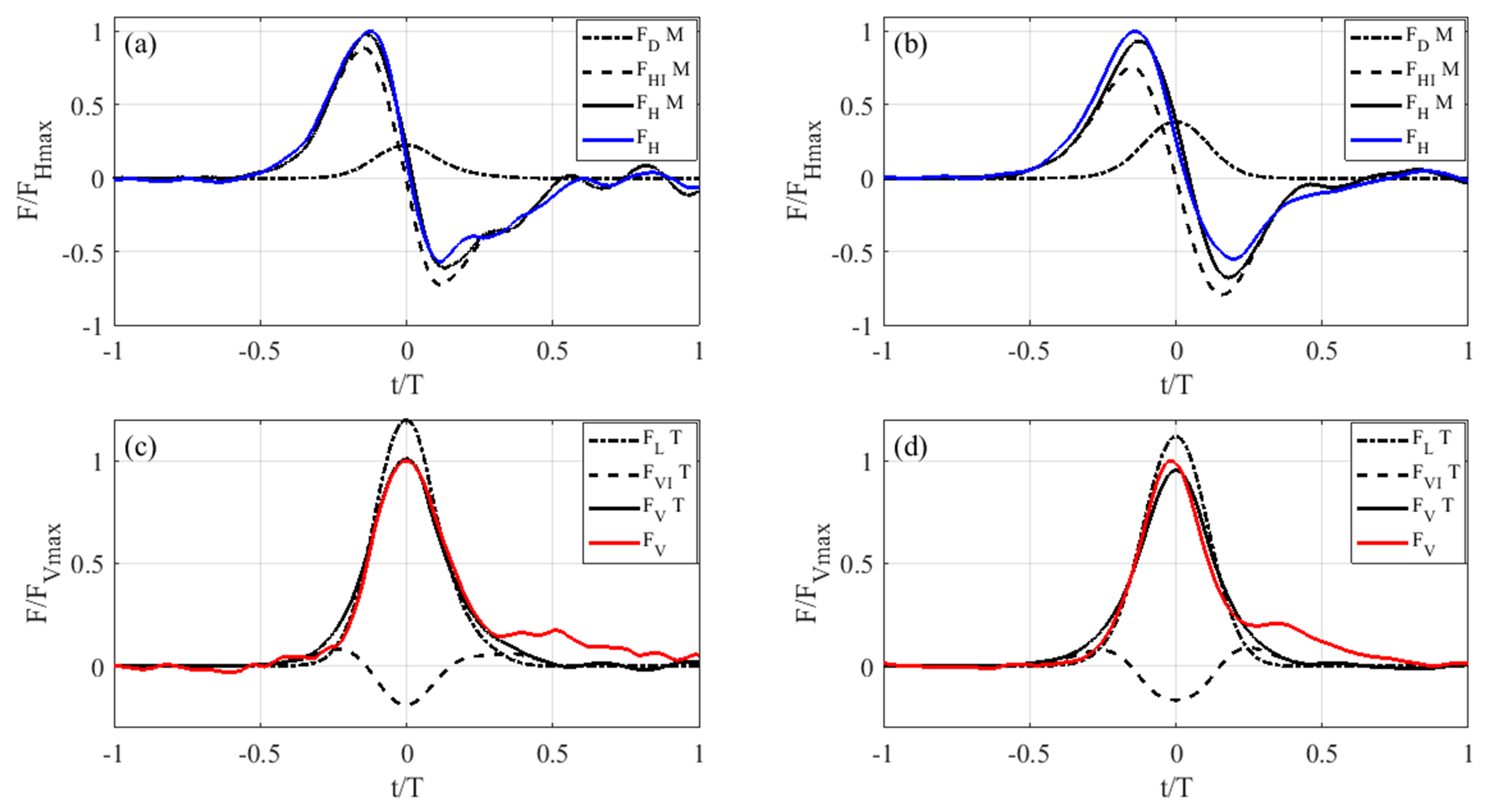
The Morison and transverse equations calibrated by experimental values of , , , and and deduced from OLS approach are here illustrated in the time domain to highlight the features of the different force components in horizontal (drag and inertia) and vertical (lift and inertia) directions. For the considered test (case numbers 5 and 30 shown in Figure 5), Figure 10a,b respectively describe the comparisons between the time variation of the drag () and inertia () as force components, and the total force () determined by the calibrated Morison equation (see Equation (9)) and the horizontal one () deduced through the laboratory experiments. For the same tests, Figure 10c,d respectively show the comparisons between the time history of the lift () and inertia () force components, and the total () determined by the calibrated transverse equation (see Equation (10)) and the vertical one () calculated by the laboratory experiments. It is worth noting that Morison and transverse component and total forces are respectively specified through the symbols M and T in Figure 10. An overall good agreement between semi-empirical methods and experiments is noted. This is evident particularly for the maximum positive peak of the horizontal and vertical force modelled by the Morison and transverse scheme for test number 5, respectively. A less accurate reproduction of the time variation of the experimental loads can be observed for the negative peak of the horizontal force, particularly for test number 30, related to the higher solitary wave. With regard to the phase shifts linked to the force peaks, the Morison and transverse forces are lower and forward-shifted as compared to the experimental ones, particularly for test number 30. This is linked to the complex patterns of vortical structures around the cylinder that are not included in the simple expressions of the adopted semi-empirical schemes. It can be noted that the horizontal force is dominated by the inertia contribution depending on the undisturbed horizontal acceleration if compared to the drag, which is related to the free stream horizontal velocity. The vertical force field is conversely dominated by the lift force and the effect of the vertical inertia is linked to a lowering of the former contribution to give the modelling of the vertical load. In general, the shape of the vertical force follows that related to the ambient horizontal velocity in which the peak is substantially in phase with the surface elevation. Owing to the presence of spurious trailing waves, it is also possible to observe a low contribution of a positive vertical load in its final part that is not modelled by the transverse scheme.
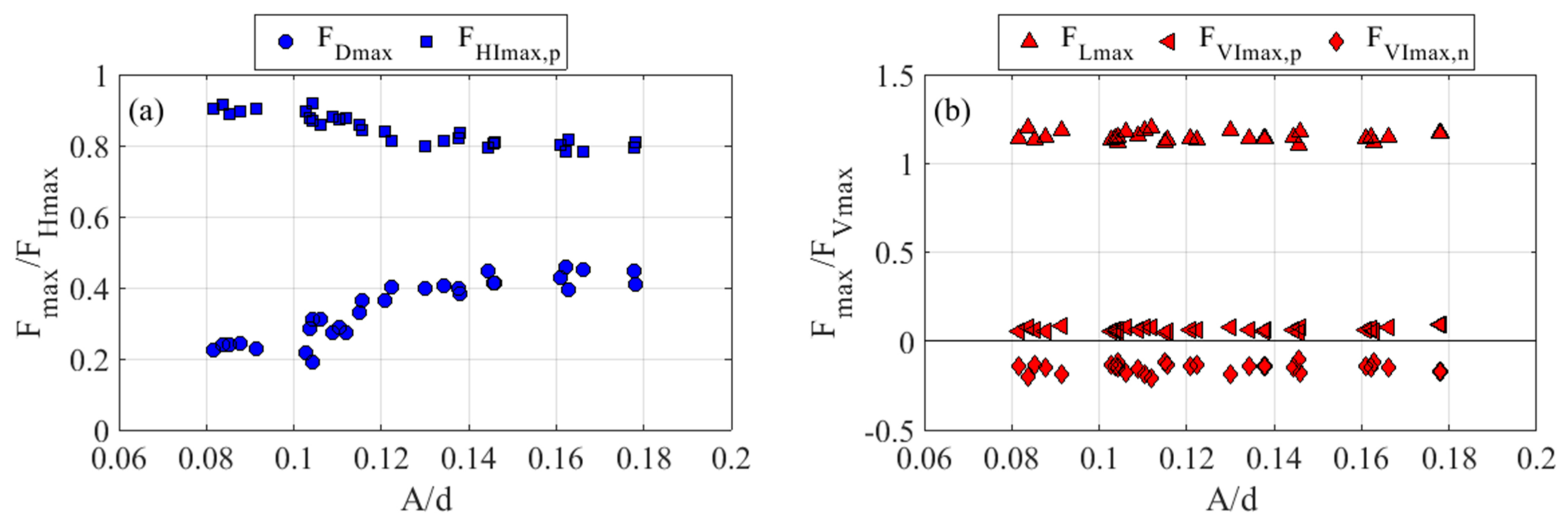
The four force components, i.e., , , , and used to calculate the total horizontal and vertical loads using the calibrated Morison and transverse formulas through the present laboratory experiments are also analysed in terms of positive and negative peaks. As highlighted in Figure 11 as a function of , the force components are weighted with respect to the corresponding maximum peak of the semi-empirical horizontal and vertical force in order to show their contribution to model the total loads. For the peaks of horizontal forces (see Figure 11a), the inertia component ranges about from 90% for low to 80% for high , leading to a progressive reduction of an inertia-dominated regime and a growth of the weight of the drag up to 45%. Paying attention to the peaks of vertical loads (see Figure 11b), a major role is linked to the maximum lift force, , which shows a slight decrease when increases. It can be observed that the ratio between the peaks of the lift component and the total vertical one is generally greater than 1. The weight of the positive () and negative () peaks compared to the maximum vertical force is quite low. Both contributions exhibit a very small increase when increases. Specifically, the values of range about from 5 to 9%, while the values of range about from 10 to 20%. It is worth noting that the tendencies of the force peaks generally reflect the features of the hydrodynamic coefficients, as illustrated in Figure 8.
6. Conclusions
The horizontal and vertical hydrodynamic forces induced by solitary waves on a horizontal cylinder placed on a horizontal sea bed have been investigated by means of 2D laboratory experiments. For this purpose, 30 laboratory tests were performed in a wave flume in which a battery of 12 pressure sensors allowed the hydrodynamic loads to be deduced.
In the present experimental flow regime ( ranging from about 0.08 to 0.18, 4 < < 7 and of order of 10), both the peaks and the shapes of the total wave forces are strongly influenced by the inertia component in the horizontal direction and by the lift component in the vertical direction. Concerning the force peaks, it has been observed that, for < 0.105, the positive horizontal peaks are higher than the positive vertical ones. For > 0.105, the physical process is inverted and the positive vertical peaks are greater than the positive horizontal ones. The above feature is evident for high .
To provide engineering indications, the overall good agreement between analytical solutions and laboratory tests in terms of surface elevation at the vertical section of the cylinder and free stream kinematic at the transversal axis of the considered structure has led, in conjunction with the experimental forces, to the calibration of the hydrodynamic coefficients in the Morison and transverse equations. The analysis of the hydrodynamic coefficients given by the experimental forces and the ambient kinematic field has highlighted that initially increases and then slightly decreases when increases, while , , and show an overall decreasing trend. The application of Morison and transverse schemes has led to a satisfactory evaluation of the maximum peaks and the associated phase shifts of the hydrodynamic forces, particularly for the positive peaks.
Acknowledgments
The authors would like to thank the laboratory technicians of the University of Calabria Fabio De Napoli and Salvatore Straticó (GMI Lab. of the Department of Civil Engineering), and Renato Bentrovato and Ernesto Ramundo (Department of Mechanical, Energy and Management Engineering) for their help in developing the physical model for the experiments.
Author Contributions
F.A. and G.T. conceived and designed the experiments; G.T. performed the experiments; G.T. and F.A. analyzed the data; F.A. wrote the paper; and P.V. supervised the research.
Conflicts of Interest
The authors declare no conflict of interest.
References
- Di Risio, M.; De Girolamo, P.; Bellotti, G.; Panizzo, A.; Aristodemo, F.; Molfetta, M.G.; Petrillo, A.F. Landslide-generated tsunamis runup at the coast of a conical island: New physical model experiments. J. Geophys. Res. Ocean. 2009, 114. [Google Scholar] [CrossRef]
- Schimmels, S.; Sriram, V.; Didenkulova, I. Tsunami generation in a large scale experimental facility. Coast. Eng. 2016, 110, 32–41. [Google Scholar] [CrossRef]
- Filianoti, P.; Di Risio, M. Solitary wave loads on submerged breakwater: Laboratory tests. In Proceedings of the 22nd International Offshore and Polar Engineering Conference, Rhodes, Greece, 17–22 June 2012; pp. 1–6. [Google Scholar]
- Wu, Y.-T.; Hsiao, S.-C. Propagation of solitary waves over double submerged barriers. Water 2017, 9, 917. [Google Scholar] [CrossRef]
- Sibley, P.; Coates, I.E.; Arumugam, K. Solitary wave forces on horizontal cylinders. Appl. Ocean Res. 1982, 4, 113–117. [Google Scholar] [CrossRef]
- Chian, C.; Ertekin, R.C. Diffraction of solitary waves by submerged horizontal cylinders. Wave Motion 1992, 15, 121–142. [Google Scholar] [CrossRef]
- Xiao, H.; Huang, W.; Tao, J.; Liu, C. Numerical modeling of wave-current forces acting on horizontal cylinder of marine structures by VOF method. Ocean Eng. 2013, 67, 58–67. [Google Scholar] [CrossRef]
- Sarpkaya, T.; Isaacson, M. Mechanics of Wave Forces on Offshore Structures; Van Nostrand Reinhold Company: New York, NY, USA, 1981; pp. 1–650. [Google Scholar]
- Sumer, B.M.; Fredsoe, J. Hydrodynamics Around Cylindrical Structures; Advanced Series on Coastal Engineering; World Scientific: Singapore, 2006; pp. 1–546. [Google Scholar]
- Morison, J.R.; O’Brien, M.P.; Johnson, J.W.; Schaaf, S.A. The forces exerted by surface waves on piles. Pet. Trans. 1950, 189, 149–156. [Google Scholar] [CrossRef]
- Grace, R.A.; Zee, G.T.Y. Wave forces on rigid pipes using ocean test data. J. Waterw. Port Coast. Ocean Eng. 1981, 107, 71–92. [Google Scholar]
- Sarpkaya, T.; Rajabi, F. Hydrodynamic drag on bottom-mounted smooth and rough cylinders in periodic flow. In Proceedings of the 11th Annual Offshore Technology Conference, Houston, TX, USA, 5–8 May 1980; pp. 219–226. [Google Scholar]
- Cheong, H.F.; Jothi-Shankar, N.; Subbiah, K. Inertia dominated forces on submarine pipelines near seabed. J. Hydraul. Res. 1989, 27, 5–22. [Google Scholar] [CrossRef]
- Bryndum, M.B.; Jacobsen, V.; Tsahalis, D.T. Hydrodynamic forces on pipelines: model tests. J. Offshore Mech. Arct. Eng. 1992, 114, 231–241. [Google Scholar] [CrossRef]
- Neill, I.A.R.; Hinwood, J.B. Wave and wave-current load on a bottom-mounted circular cylinder. Int. J. Offshore Polar 1998, 2, 122–129. [Google Scholar]
- Chevalier, C.; Lambert, E.; Bélorgey, M. Efforts sur une conduite sous-marine en zone côtière. Revue Française de Génie Civil 2001, 5, 995–1014. (In French) [Google Scholar] [CrossRef]
- Aristodemo, F.; Tomasicchio, G.R.; Veltri, P. Modelling of periodic and random wave forces on submarine pipelines. In Proceedings of the 25th International Conference on Mechanics and Arctic Engineering, Hamburg, Germany, 4–9 June 2006; pp. 1–10. [Google Scholar]
- Det Norske Veritas. DNV-RP-F109, On-Bottom Stability Design of Offshore Pipelines; Det Norske Veritas: Hovik, Norway, 2010; pp. 1–41. [Google Scholar]
- Aristodemo, F.; Tomasicchio, G.R.; Veltri, P. Wave and current forces at a bottom-mounted submarine pipeline. J. Coast. Res. 2013, 65, 153–158. [Google Scholar] [CrossRef]
- Aristodemo, F.; Tomasicchio, G.R.; Veltri, P. New model to determine forces at on-bottom slender pipelines. Coast. Eng. 2011, 58, 267–280. [Google Scholar] [CrossRef]
- Kuznetsov, K.I.; Harris, J.; Germain, N.; Aristodemo, F. Modification of a Wake Model for Hydrodynamic Forces on Submarine Cables with a Rough Seabed; EGU2018-19847; Geophysical Research Abstracts: Vienna, Austria, 2018; Volume 20. [Google Scholar]
- Aristodemo, F.; Tripepi, G.; Meringolo, D.D.; Veltri, P. Solitary wave-induced forces on horizontal circular cylinders: Laboratory experiments and SPH simulations. Coast. Eng. 2017, 129, 17–35. [Google Scholar] [CrossRef]
- Liu, X.; Lin, P.; Shao, S. An ISPH simulation of coupled structure interaction with free surface flows. J. Fluids Struct. 2014, 48, 46–61. [Google Scholar] [CrossRef]
- Aristodemo, F.; Meringolo, D.D.; Groenenboom, P.; Lo Schiavo, A.; Veltri, P.; Veltri, M. Assessment of dynamic pressures at vertical and perforated breakwaters through diffusive SPH schemes. Math. Prob. Eng. 2015, 2015, 305028. [Google Scholar] [CrossRef]
- Aristodemo, F.; Marrone, S.; Federico, I. SPH modeling of plane jets into water bodies through an inflow/outflow algorithm. Ocean Eng. 2015, 105, 160–175. [Google Scholar] [CrossRef]
- Gui, Q.; Dong, P.; Shao, S. Numerical study of PPE source term errors in the incompressible SPH models. Int. J. Num. Methods Fluids 2015, 77, 358–379. [Google Scholar] [CrossRef]
- Shadloo, M.S.; Weiss, R.; Yildiz, M.; Dalrymple, R.A. Numerical simulation of long wave runup for breaking and nonbreaking waves. Int. J. Offshore Polar Eng. 2015, 25, 1–7. [Google Scholar]
- Shadloo, M.S.; Oger, G.; Le Touzé, D. Smoothed particle hydrodynamics method for fluid flows, towards industrial applications: Motivations, current state, and challenges. Comput. Fluids 2016, 136, 11–34. [Google Scholar] [CrossRef]
- Nasiri, H.; Jamalabadi, M.Y.A.; Sadeghi, R.; Safaei, M.R.; Nguyen, T.K.; Shadloo, M.S. A smoothed particle hydrodynamics approach for numerical simulation of nano-fluid flows: Application to forced convection heat transfer over a horizontal cylinder. J. Therm. Anal. Calorim. 2018, 1–9. [Google Scholar] [CrossRef]
- Rayleigh, L. On waves. Phil. Mag. 1876, 1, 257–279. [Google Scholar]
- Guizien, K.; Barthélemy, E. Accuracy of solitary wave generation by a piston wave maker. J. Hydraul. Res. 2002, 40, 321–331. [Google Scholar]
- Dingemans, M.W. Water Wave Propagation Over Uneven Bottoms; Advanced Series on Coastal Engineering; World Scientific: Singapore, 1997; pp. 1–703. [Google Scholar]
- Madsen, P.A.; Fuhrman, D.R.; Schäffer, H.A. On the solitary wave paradigm for tsunamis. J. Geophys. Res. 2008, 113, C12012. [Google Scholar] [CrossRef]
- Lee, J.J.; Skjelbreia, J.E.; Raichlen, F. Measurements of velocities in solitary waves. J. Waterw. Port Coast. Ocean Eng. 1982, 108, 200–218. [Google Scholar]
- Tripepi, G.; Aristodemo, F.; Veltri, P.; Pace, C.; Solano, A.; Giordano, C. Experimental and numerical investigation of tsunami-like waves on horizontal circular cylinders. In Proceedings of the 36th International Conference on Ocean, Offshore and Arctic Engineering, Trondheim, Norway, 25–30 June 2017; pp. 1–10. [Google Scholar]
- Mattioli, M.; Mancinelli, A.; Brocchini, M. Experimental investigation of the wave-induced flow around a surface-touching cylinder. J. Fluids Struct. 2013, 37, 62–87. [Google Scholar] [CrossRef]
- Lin, M.Y.; Liao, G.Z. Vortex shedding around a near-wall circular cylinder induced by a solitary wave. J. Fluids Struct. 2015, 58, 127–151. [Google Scholar] [CrossRef]
- Filianoti, P.; Aristodemo, F.; Tripepi, G.; Gurnari, L. Wave flume test to check a semi-analytical method for calculating solitary wave loads on horizontal cylinders. In Proceedings of the 36th International Conference on Ocean, Offshore and Arctic Engineering, Trondheim, Norway, 25–30 June 2017; pp. 1–9. [Google Scholar]
- Seiffert, B.; Hayatdavoodi, M.; Ertekin, R.C. Experiments and computations of solitary-wave forces on a coastal-bridge deck. Part I: Flat Plate. Coast. Eng. 2014, 88, 194–209. [Google Scholar] [CrossRef]
- Wolfram, J.; Naghipour, M. On the estimation of Morison force coefficients and their predictive accuracy for very rough circular cylinders. Appl. Ocean Res. 1999, 21, 311–328. [Google Scholar] [CrossRef]
- Sumer, B.M.; Jensen, B.L.; Fredsoe, J. Effect of a plane boundary on oscillatory flow around a circular cylinder. J. Fluid Mech. 1991, 225, 271–300. [Google Scholar] [CrossRef]
Figure 1.
Sketch of the longitudinal profile of the experimental setup.
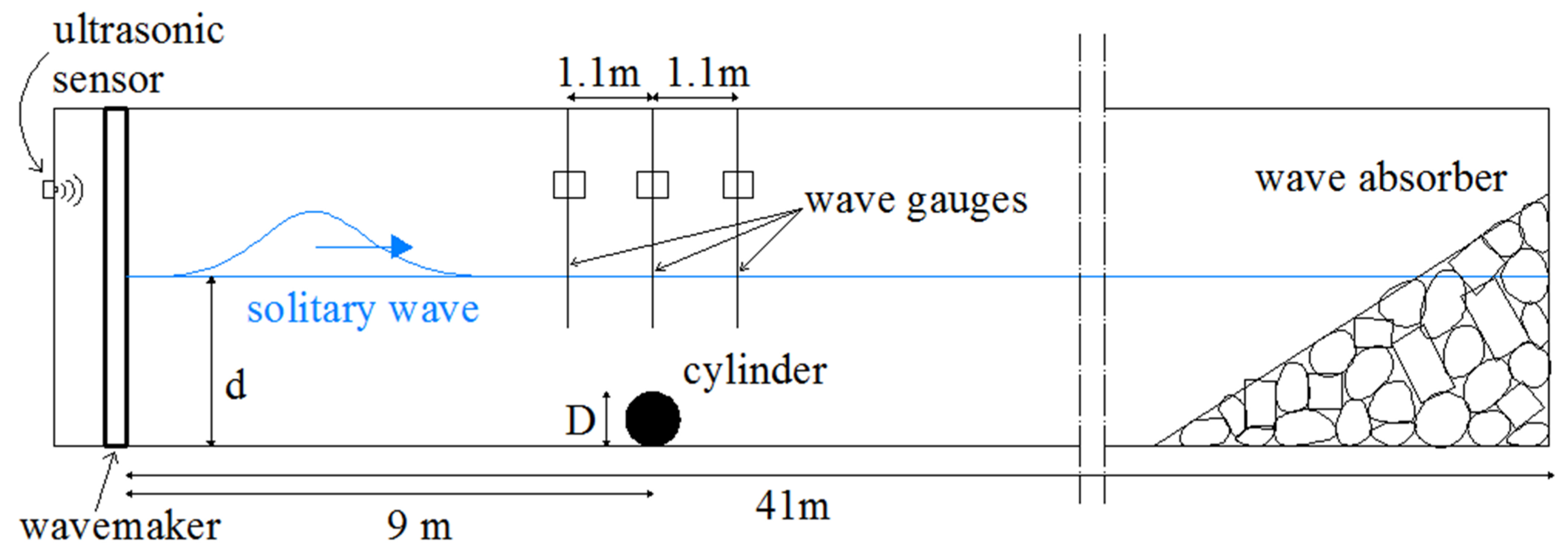
Figure 2.
(a) Front view from the paddle of the cylinder and the staggered transducer arrangement in the wave channel; (b) View of the cylinder placement during the experiments; (c) Representative cross section of the transducers around the bottom-mounted cylinder.
Figure 2.
(a) Front view from the paddle of the cylinder and the staggered transducer arrangement in the wave channel; (b) View of the cylinder placement during the experiments; (c) Representative cross section of the transducers around the bottom-mounted cylinder.
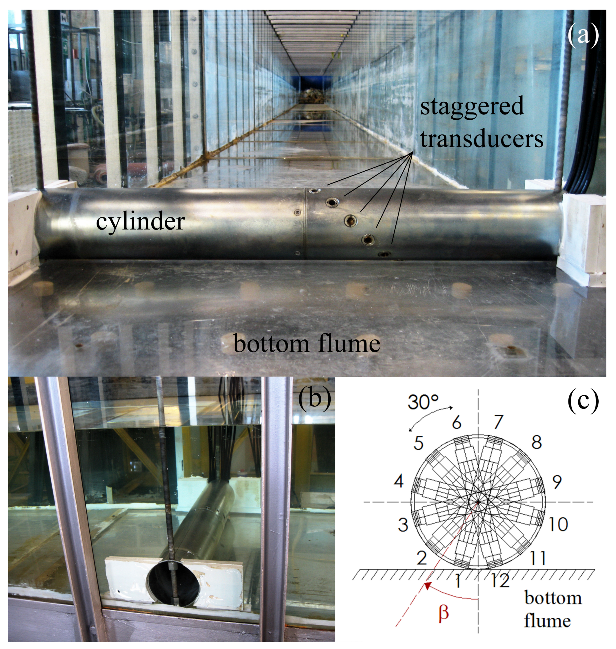
Figure 3.
Time variation of surface elevation, , in correspondence to the vertical axis of the cylinder: comparison between analytical solution and experiments. (a) Test number 5; (b) Test number 30.
Figure 3.
Time variation of surface elevation, , in correspondence to the vertical axis of the cylinder: comparison between analytical solution and experiments. (a) Test number 5; (b) Test number 30.
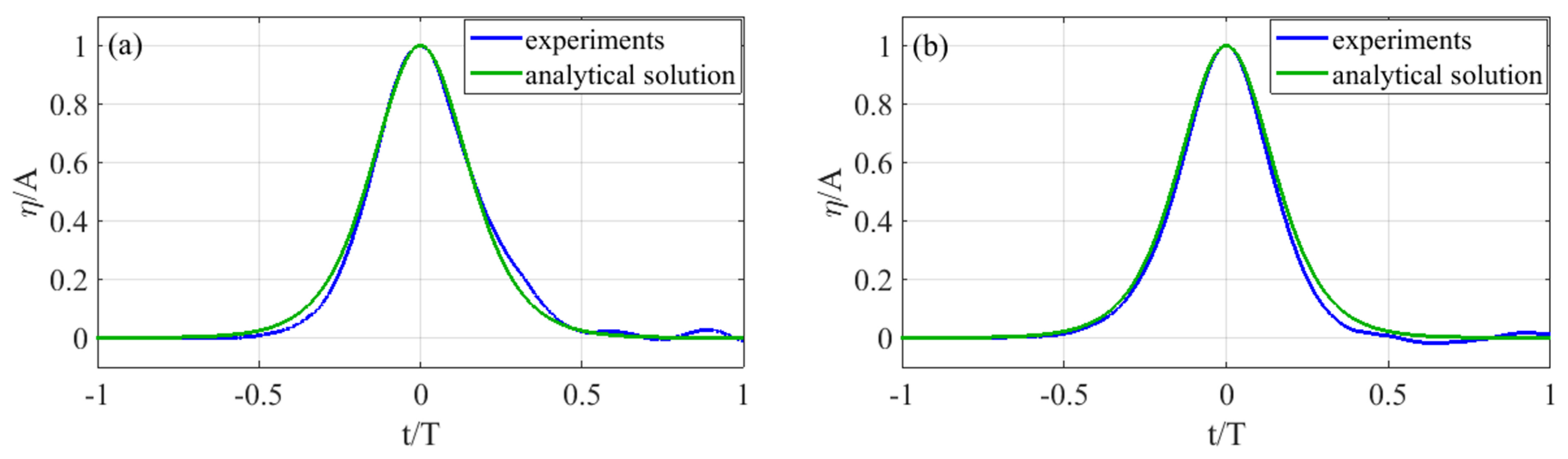
Figure 4.
Time variation of undisturbed kinematic field at the transversal axis of the cylinder: comparison between analytical solution and experiments (test number 30). (a) Horizontal velocity, u; (b) Horizontal acceleration, ; (c) Vertical acceleration, .
Figure 4.
Time variation of undisturbed kinematic field at the transversal axis of the cylinder: comparison between analytical solution and experiments (test number 30). (a) Horizontal velocity, u; (b) Horizontal acceleration, ; (c) Vertical acceleration, .
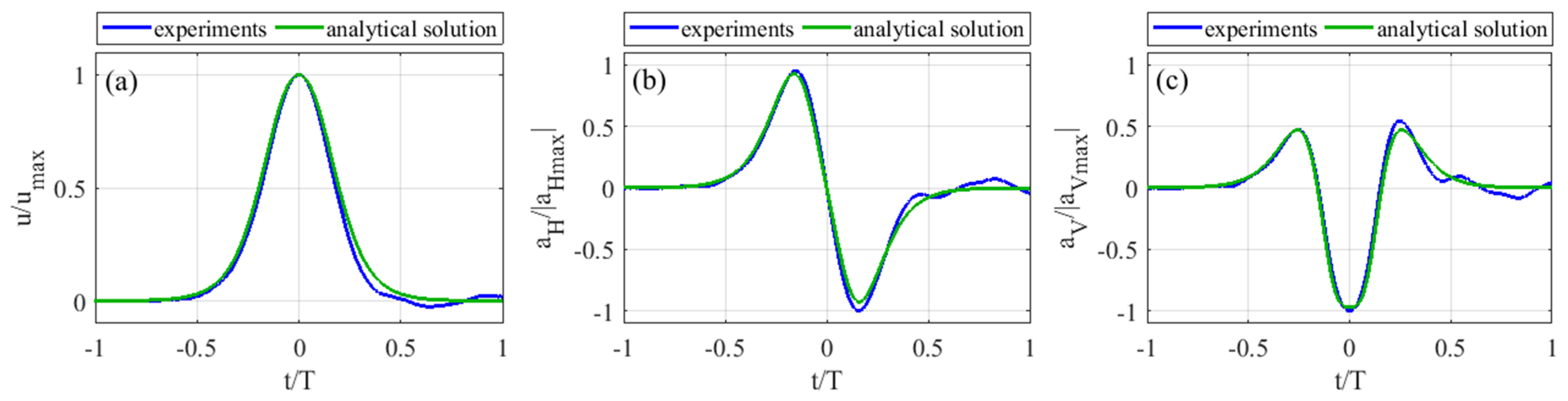
Figure 5.
Time variation of experimental horizontal () and vertical () hydrodynamic forces. (a) Test number 5; (b) Test number 30.
Figure 5.
Time variation of experimental horizontal () and vertical () hydrodynamic forces. (a) Test number 5; (b) Test number 30.

Figure 6.
Maximum positive and negative peaks of experimental horizontal forces ( and , respectively), and maximum positive peaks of experimental vertical forces ( ), vs. .
Figure 6.
Maximum positive and negative peaks of experimental horizontal forces ( and , respectively), and maximum positive peaks of experimental vertical forces ( ), vs. .
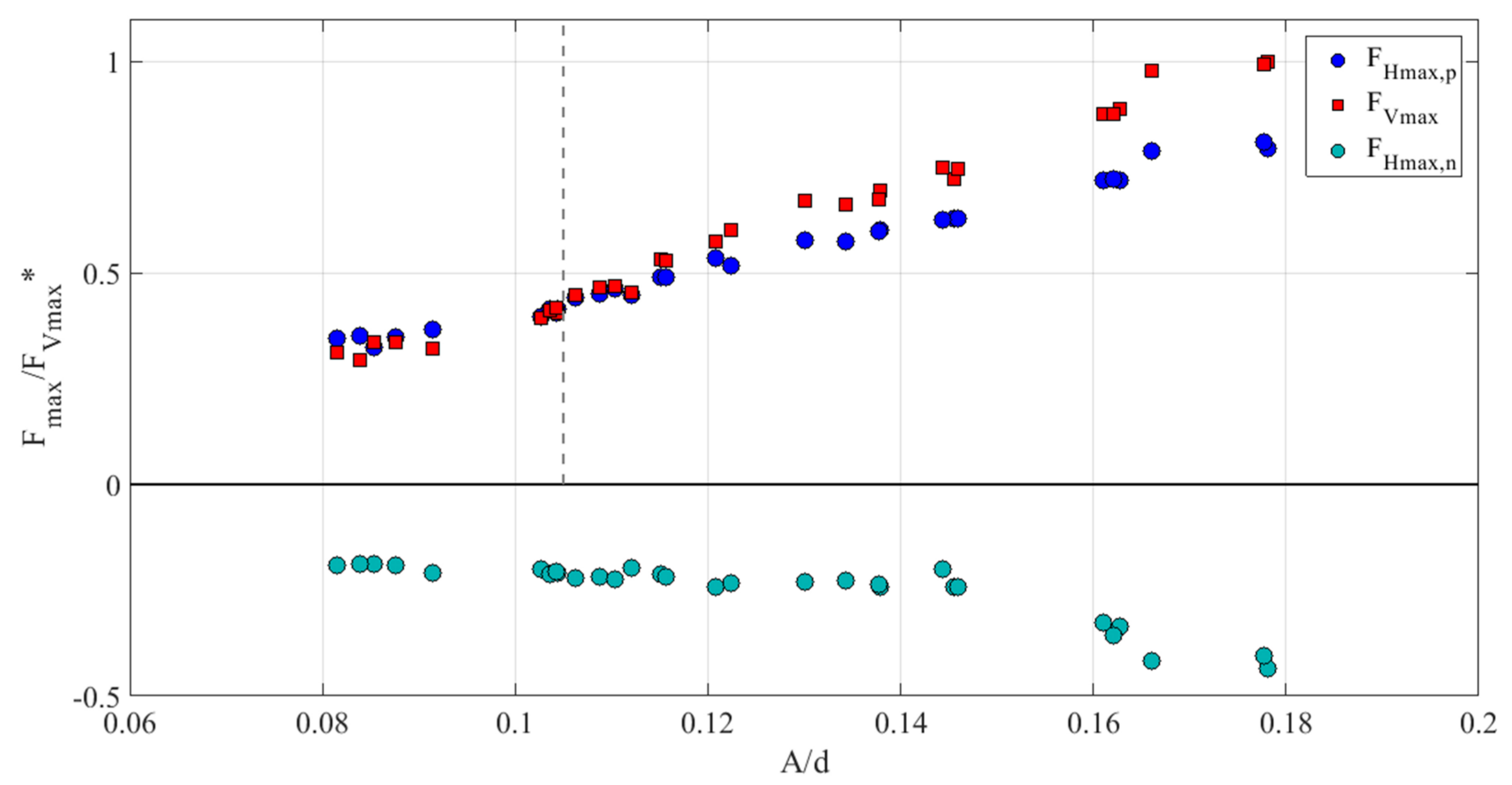
Figure 7.
Experimental mean square error percent (MSEP) through OLS, WLS1, WLS2, WLS3, WLS4, WLS5, and WLS6 methods. (a) Maximum positive horizontal force, ; (b) Maximum negative horizontal force, ; (c) Maximum vertical force, ; (d) Phase shift, , associated with ; (e) Phase shift, , associated with ; (f) Phase shift, , associated with . OLS: ordinary least square; WLS: weighted least square.

Figure 8.
Experimental hydrodynamic coefficients vs. . (a) ; (b) ; (c) ; (d) .

Figure 9.
Experimental hydrodynamic coefficients vs. and comparison with literature coefficients for regular waves. (a) ; (b) ; (c) .
Figure 9.
Experimental hydrodynamic coefficients vs. and comparison with literature coefficients for regular waves. (a) ; (b) ; (c) .
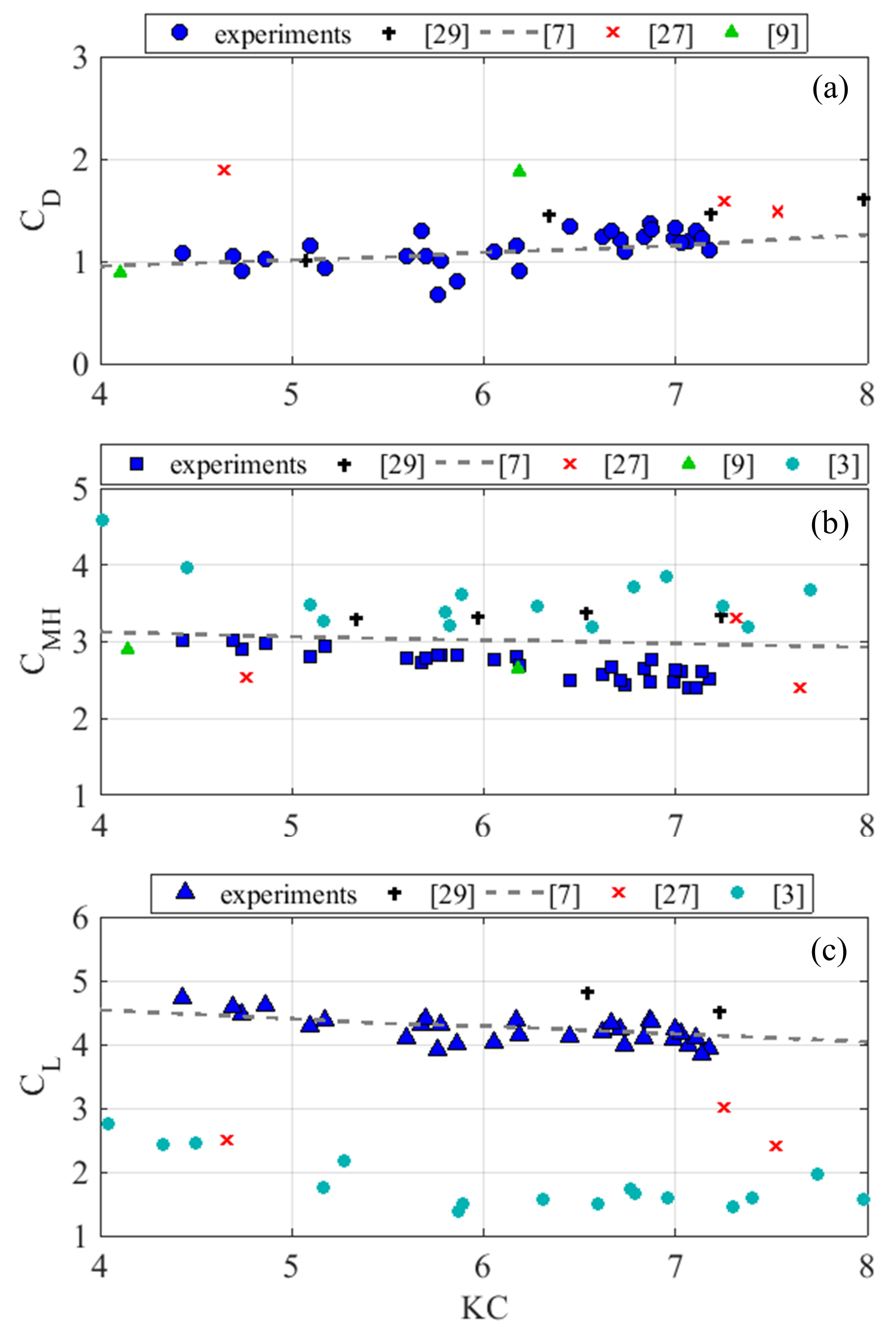
Figure 10.
Time history of hydrodynamic loads determined by semi-empirical formulas and experiments. (a) Comparison between Morison , , and calibrated by experiments and experimental (test number 5); (b) Comparison between Morison , , and calibrated by experiments and experimental (test number 30); (c) Comparison between transverse , , and calibrated by experiments and experimental (test number 5); (d) Comparison between transverse , , and calibrated by experiments and experimental (test number 30).

Figure 11.
(a) Peaks of experimental Morison force components vs. : positive drag and positive inertia ; (b) Peaks of experimental transverse force components vs. : positive lift , positive inertia , and negative inertia .
Figure 11.
(a) Peaks of experimental Morison force components vs. : positive drag and positive inertia ; (b) Peaks of experimental transverse force components vs. : positive lift , positive inertia , and negative inertia .


Table 1.
Characteristics of the experimental tests.
| Test Number | A (m) | T (s) | A/d | KC | Re | d/L |
|---|---|---|---|---|---|---|
| 1 | 0.033 | 3.73 | 0.083 | 4.43 | 1.83 × 10⁴ | 0.052 |
| 2 | 0.034 | 3.84 | 0.085 | 4.69 | 1.87 × 10⁴ | 0.051 |
| 3 | 0.034 | 3.82 | 0.085 | 4.74 | 1.91 × 10⁴ | 0.051 |
| 4 | 0.035 | 3.83 | 0.088 | 4.86 | 1.95 × 10⁴ | 0.051 |
| 5 | 0.037 | 3.91 | 0.093 | 5.17 | 2.03 × 10⁴ | 0.050 |
| 6 | 0.041 | 3.99 | 0.103 | 5.86 | 2.26 × 10⁴ | 0.048 |
| 7 | 0.041 | 3.78 | 0.103 | 5.60 | 2.27 × 10⁴ | 0.051 |
| 8 | 0.042 | 3.87 | 0.105 | 5.76 | 2.29 × 10⁴ | 0.050 |
| 9 | 0.042 | 4.06 | 0.105 | 6.06 | 2.29 × 10⁴ | 0.047 |
| 10 | 0.043 | 3.37 | 0.108 | 5.10 | 2.33 × 10⁴ | 0.057 |
| 11 | 0.044 | 3.73 | 0.110 | 5.77 | 2.38 × 10⁴ | 0.051 |
| 12 | 0.044 | 3.64 | 0.110 | 5.70 | 2.41 × 10⁴ | 0.053 |
| 13 | 0.045 | 3.90 | 0.113 | 6.19 | 2.44 × 10⁴ | 0.049 |
| 14 | 0.046 | 3.79 | 0.115 | 6.17 | 2.50 × 10⁴ | 0.050 |
| 15 | 0.046 | 3.47 | 0.115 | 5.67 | 2.51 × 10⁴ | 0.055 |
| 16 | 0.048 | 4.05 | 0.120 | 6.87 | 2.61 × 10⁴ | 0.047 |
| 17 | 0.049 | 3.88 | 0.123 | 6.66 | 2.64 × 10⁴ | 0.049 |
| 18 | 0.052 | 3.86 | 0.130 | 7.00 | 2.78 × 10⁴ | 0.049 |
| 19 | 0.054 | 3.56 | 0.135 | 6.62 | 2.86 × 10⁴ | 0.053 |
| 20 | 0.055 | 3.59 | 0.138 | 6.84 | 2.92 × 10⁴ | 0.053 |
| 21 | 0.055 | 3.69 | 0.138 | 7.03 | 2.93 × 10⁴ | 0.051 |
| 22 | 0.058 | 3.26 | 0.145 | 6.45 | 3.04 × 10⁴ | 0.058 |
| 23 | 0.058 | 3.58 | 0.145 | 7.14 | 3.06 × 10⁴ | 0.053 |
| 24 | 0.058 | 3.36 | 0.145 | 6.71 | 3.07 × 10⁴ | 0.056 |
| 25 | 0.064 | 3.22 | 0.160 | 6.99 | 3.33 × 10⁴ | 0.058 |
| 26 | 0.065 | 3.26 | 0.163 | 7.11 | 3.35 × 10⁴ | 0.058 |
| 27 | 0.065 | 3.28 | 0.163 | 7.18 | 3.36 × 10⁴ | 0.057 |
| 28 | 0.066 | 3.09 | 0.165 | 6.87 | 3.42 × 10⁴ | 0.061 |
| 29 | 0.071 | 3.01 | 0.178 | 7.07 | 3.61 × 10⁴ | 0.062 |
| 30 | 0.071 | 2.86 | 0.178 | 6.74 | 3.62 × 10⁴ | 0.065 |
© 2018 by the authors. Licensee MDPI, Basel, Switzerland. This article is an open access article distributed under the terms and conditions of the Creative Commons Attribution (CC BY) license (http://creativecommons.org/licenses/by/4.0/).
Share and Cite
MDPI and ACS Style
Tripepi, G.; Aristodemo, F.; Veltri, P. On-Bottom Stability Analysis of Cylinders under Tsunami-Like Solitary Waves. Water 2018, 10, 487. https://doi.org/10.3390/w10040487
AMA Style
Tripepi G, Aristodemo F, Veltri P. On-Bottom Stability Analysis of Cylinders under Tsunami-Like Solitary Waves. Water. 2018; 10(4):487. https://doi.org/10.3390/w10040487
Chicago/Turabian StyleTripepi, Giuseppe, Francesco Aristodemo, and Paolo Veltri. 2018. "On-Bottom Stability Analysis of Cylinders under Tsunami-Like Solitary Waves" Water 10, no. 4: 487. https://doi.org/10.3390/w10040487
Note that from the first issue of 2016, this journal uses article numbers instead of page numbers. See further details here.